Chiral transition, eigenmode localisation and Anderson-like models

Abstract:

We discuss chiral symmetry restoration and eigenmode localisation in finite-temperature QCD by looking at the lattice Dirac operator as a random Hamiltonian. We argue that the features of QCD relevant to both phenomena are the presence of order in the Polyakov line configuration, and the correlations that this induces between spatial links across time slices. This ties the fate of chiral symmetry and of localisation of the lowest Dirac eigenmodes to the confining properties of the theory. We then show numerical results obtained in a QCD-inspired Anderson-like toy model, derived by radically simplifying the QCD dynamics while keeping the important features mentioned above. The toy model reproduces all the important qualitative aspects of chiral symmetry breaking and localisation in QCD, thus supporting the central role played by the confinement/deconfinement transition in triggering both phenomena.

1 Introduction

As is well known, in QCD both the confining and chiral properties of the theory undergo a rapid change around a temperature $T_{c}\simeq 155~{}{\rm MeV}$ [1]. Moreover, in models where there is a genuine phase transition, rather than just an analytic crossover like in QCD, deconfinement and the chiral transition take place at the same temperature. Such models include SU$(2)$ and SU$(3)$ pure gauge theory, SU$(3)$ gauge theory with uninmproved staggered fermions on $N_{T}=4$ lattices [2], and SU$(3)$ gauge theory with adjoint fermions [3]. A convincing explanation of why deconfinement and the chiral transition take place together is still lacking.

In recent years there has been growing evidence of a third phenomenon taking place in QCD around $T_{c}$, namely the change in the localisation properties of the low-lying eigenmodes of the Dirac operator [4, 5, 6, 7, 8, 9, 10, 11]. While below $T_{c}$ all the modes are delocalised [12], above $T_{c}$ the lowest modes are spatially localised on the scale of the inverse temperature, up to a critical, temperature-dependent point $\lambda_{c}(T)$ in the spectrum (“mobility edge”); modes above $\lambda_{c}$ are again delocalised. The localisation/delocalisation transition at the mobility edge is a second-order phase transition with divergent correlation length [9]. Extrapolating $\lambda_{c}(T)$ as $T$ is decreased, one finds that $\lambda_{c}(T)$ vanishes at a temperature compatible with $T_{c}$. The low-lying modes play a crucial role in physical observables, in particular in the formation of a chiral condensate, and therefore for the spontaneous breaking of chiral symmetry (S$\chi$SB). It is therefore not so surprising that the localisation properties of these modes change at the chiral transition.

The appearance of localised modes in the deconfined/chirally restored phase is not a unique feature of QCD, but has been observed also in other QCD-like models [4, 6, 13]. In models where the transition is sharp one can ask more meaningfully whether localisation appears right at the critical point. In the above-mentioned model with unimproved staggered fermions [2], which displays a first-order deconfining and chiral transition, the onset of localisation has been shown to take place precisely at the critical temperature [13]. Understanding localisation might therefore help in understanding the relation between deconfinement and the chiral transition.

2 QCD, the Anderson Model and the Dirac-Anderson Hamiltonian

The best known model displaying localisation of eigenmodes is the celebrated Anderson model (AM) [14], which provides an approximate description of (non-interacting) electrons in “dirty” conductors. The effect of impurities is modelled by a random on-site potential, added to the usual hopping terms of the tight-binding Hamiltonian; the amount of impurities/disorder is controlled by the width $W$ of the range in which the random potential takes its values. In the AM, eigenmodes at the band edge are localised, for energies beyond the so-called mobility edge, and the localisation/delocalisation transition within the spectrum is a second-order phase transition with divergent correlation length. Concerning localisation of the eigenmodes, QCD and the AM are thus completely analogous. Since in the AM the position of the mobility edge is determined by $W$, while in QCD it is controlled by the temperature $T$, one is led to identify $T$ as the parameter effectively controlling the amount of disorder in QCD. There is, however, more than a simple analogy between the two models. In fact, the correlation-length critical exponent in QCD was found to be compatible [9] with that of the 3D unitary AM [15]. Here “unitary” refers to the symmetry class of the model in the classification of Random Matrix Theory (RMT) [12]. Moreover, eigenmodes at the mobility edge are multifractal [10], with multifractal exponents matching those of the 3D unitary AM [16]. These results have been obtained using the staggered discretisation of the Dirac operator.

The fact that the transitions in the two models share the same universality class calls for an explanation. From the point of view of RMT, the QCD staggered Dirac operator is a random matrix of the unitary class, with off-diagonal noise provided by the fluctuations of the gauge links. Moreover, QCD at finite temperature is a 4D model. The unitary AM, on the other hand, is 3D with mostly diagonal disorder. A qualitative explanation for the matching of universality classes is the following [7, 17, 18]. For $T>T_{c}$ time-slices are strongly correlated, QCD is effectively 3D, and the quark eigenfunctions $\psi(t,{\vec{x}})$ are expected to look qualitatively the same on all the time-slices. Moreover, working in the temporal gauge, one sees that $\psi(t,{\vec{x}})$ obeys effective boundary conditions in the temporal direction, which involve the local Polyakov line (PL), $P(\vec{x})$, namely $\psi(N_{T},{\vec{x}})=-P({\vec{x}})\psi(0,{\vec{x}})$. Here $N_{T}$ is the temporal extension of the system in lattice units. Since $P(\vec{x})$ fluctuates in space, it provides an effective 3D source of diagonal disorder. This explanation leads, however, to another question. The effective boundary conditions apply both above and below $T_{c}$, and similarly the PL fluctuates in space in both phases of the theory. One thus has to justify why QCD is effectively 4D at low $T$, and why the effective boundary conditions are ineffective there.

In order to better understand the relation between QCD and the unitary AM, following Ref. [18], we make the connection explicit between the staggered Dirac operator $D_{\rm stag}$ and Anderson-type Hamiltonians. We start from the “Hamiltonian” $H=-iD_{\rm stag}$, split it into a “free” and an “interaction” part, $H=H_{0}+H_{I}$, and then work in the basis of the “unperturbed” eigenvectors of $H_{0}$. The physically most sensible choice is to identify $H_{0}$ with the temporal hoppings, $(H_{0})_{xx^{\prime}}={\textstyle\frac{\eta_{4}(\vec{x})}{2i}}[U_{4}(t,\vec{x})\delta_{t+1,t^{\prime}}-U_{-4}(t,\vec{x})\delta_{t-1,t^{\prime}}]\delta_{\vec{x},\vec{x}{}^{\prime}}$, thus leaving the spatial hoppings as the spatially isotropic interaction part, $(H_{I})_{xx^{\prime}}=\textstyle\sum_{j=1}^{3}{\textstyle\frac{\eta_{j}(\vec{x})}{2i}}[U_{j}(t,\vec{x})\delta_{\vec{x}+\hat{\jmath},\vec{x}{}^{\prime}}-U_{-j}(t,x)\delta_{\vec{x}-\hat{\jmath},\vec{x}{}^{\prime}}]\delta_{t,t^{\prime}}$. Here $x=(t,\vec{x})$, $U_{\mu}(x)=U_{\mu}(t,\vec{x})$ are SU$(N_{c})$ gauge links with $U_{-\mu}(x)=U^{\dagger}_{\mu}(x-\hat{\mu})$, and $\eta_{\mu}(\vec{x})$ are the usual staggered phases. In the temporal diagonal gauge one has $U_{4}=\mathbf{1}$ $\forall t\neq N_{T}-1$, and $U_{4}(N_{T}-1,\vec{x})=P(\vec{x})={\rm diag}(e^{i\phi_{a}(\vec{x})})$, $a=1,\ldots,N_{c}$, having diagonalised each PL with a time-independent gauge transformation. We choose $\sum_{a}\phi_{a}(\vec{x})=0$, any other choice leading to a unitarily equivalent Hamiltonian. In this gauge it is straightforward to diagonalise $H_{0}$, finding for the unperturbed eigenvalues

$$\lambda_{0}^{\vec{x}\,a\,k}=\eta_{4}(\vec{x})\sin\omega_{ak}(\vec{x})\,,\quad\omega_{ak}(\vec{x})={\textstyle\frac{1}{N_{T}}}(\pi+\phi_{a}(\vec{x})+2\pi k)\,,$$ (1)

where $\omega_{ak}(\vec{x})$ are the effective Matsubara frequencies. The various indices refer to the spatial site $\vec{x}$ where the eigenmode is localised, and the colour component $a$ and the temporal momentum (TM) $k=0,\ldots,N_{T}-1$ to which it corresponds. In the basis of the unperturbed eigenvectors one finds

$${H}_{\vec{x},\vec{y}} =\textstyle\delta_{\vec{x},\vec{y}}D(\vec{x})+\sum_{j=1}^{3}\frac{\eta_{j}(\vec{x})}{2i}\left[\delta_{\vec{x}+\hat{\jmath},\vec{y}}V_{+j}(\vec{x})-\delta_{\vec{x}-\hat{\jmath},\vec{y}}V_{-j}(\vec{x})\right]\,,$$ (2)

$$\left[D(\vec{x})\right]_{ak,bl} =\lambda_{0}^{\vec{x}\,a\,k}\delta_{ab}\delta_{kl}\,,$$

$$\left[V_{\pm j}(\vec{x})\right]_{ak,bl} =\textstyle\frac{1}{N_{T}}\sum_{t=0}^{N_{T}-1}e^{i\frac{2\pi t}{N_{T}}(l-k)}e^{i\frac{t}{N_{T}}[\phi_{b}(\vec{x}\pm\hat{\jmath})-\phi_{a}(\vec{x})]}\left[{U}^{\rm(td)}_{\pm j}(t,\vec{x})\right]_{ab}\,,$$

with ${U}^{\rm(td)}_{\pm j}(t,\vec{x})$ the spatial gauge links in the temporal diagonal gauge.

The “Dirac-Anderson Hamiltonian” of Eq. (2) is a 3D Anderson-type Hamiltonian with internal degrees of freedom, corresponding to colour and TM, and including both diagonal and off-diagonal noise. Unlike the AM, here the control parameter (the temperature) does not change the overall strength of the disorder (which is always bounded in magnitude), but rather its type and its spatial distribution, which are completely different in the confined and deconfined phases of QCD.

In the deconfined phase, the PL gets ordered along $\mathbf{1}$, with fluctuations away from the ordered value forming “islands” of “wrong” PLs. This directly reduces the density of small unperturbed eigenvalues. Moreover, it leads to a reduction of the hopping terms’ entries that are off-diagonal in TM, as a consequence of the correlations among spatial links on different time-slices induced by the ordering. Since “wrong” PLs yield smaller unperturbed eigenvalues, one expects them to provide an “energetically” favourable place for the quark eigenfunctions to live on, thus allowing for smaller eigenvalues. Moreover, the mixing of different TM components is harder outside of these islands. In other words, the “islands” provide localising “traps” for the low eigenmodes. The approximate decoupling of different TM components leads to having in practice $N_{T}$ weakly coupled, effectively 3D systems. The ordering of the PLs is also expected to affect the spectral density of the low modes, and therefore the fate of chiral symmetry. Indeed, mixing of TM components tends to “push” the modes towards the origin, and its reduction, combined with a smaller density of low unperturbed modes, leads us to expect a vanishing spectral density at zero, $\rho(0)$.

In the low-$T$ phase, on the other hand, there is no spatial structure in the diagonal noise, and no strong correlations among time-slices, so no localisation is expected. The various TM components of the wave function are effectively mixed by the hopping terms, and so TM acts effectively as a fourth dimension, i.e., one deals with a single effectively 4D system. The larger density of low unperturbed modes and the fact that they can easily mix is expected to lead to a nonvanishing $\rho(0)$.

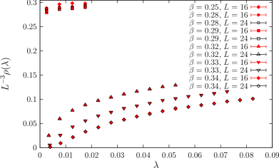
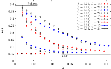
Figure 1: Spectral density $\rho$ (left) and spectral statistics $I_{0.5}$ (right) in our toy model.

Summarising, the relevant feature both for chiral symmetry restoration and localisation of the lowest modes is expected to be the ordering of the PLs. In the absence of ordering we expect instead to have S$\chi$SB and delocalisation. This ultimately links both phenomena to the confining properties of the theory, thus providing an explanation for the coincidence of the chiral transition, the onset of localisation, and deconfinement, the latter being the “fundamental” phenomenon on which the other two depend.

3 Toy model

In order to check the arguments of the previous Section, we have constructed a QCD-based toy model, keeping only the features that are expected to be relevant for chiral symmetry breaking/restoration and delocalisation/localisation of the lowest modes [18]. As we discussed above, these should be the ordering of the PLs, and the correlation between spatial links on different time slices that this induces. We thus considered a Hamiltonian with the same structure as the Dirac-Anderson Hamiltonian, Eq. (2), and replaced the PL phases $\phi_{a}(\vec{x})$ and the spatial gauge links ${U}^{\rm(td)}_{\pm j}(t,\vec{x})$ with appropriate toy-model counterparts $\phi_{\vec{x}}^{a}$ and $u_{\pm j}(t,\vec{x})$. In particular, $\phi_{\vec{x}}^{a}$ are taken to be the phases of a set of complex-spin variables, constrained by $\sum_{a}\phi_{\vec{x}}^{a}=0$, and $u_{j}(t,\vec{x})$ are SU$(N_{c})$ matrices. Writing the Dirac-Anderson Hamiltonian as a functional $H={\cal H}[\phi_{a}(\vec{x}),{U}^{\rm(td)}_{\pm j}(t,\vec{x})]$, the toy model Hamiltonian is then defined by $H^{\rm toy}={\cal H}[\phi^{a}_{\vec{x}},u_{\pm j}(t,\vec{x})]$.

The dynamics obeyed by the toy-model variables is constructed mimicking that of their counterparts in gauge theory. The important feature of the PL dynamics is the existence of an ordered and of a disordered phase. This is easily achieved for our complex spins by taking a spin model of the following form:

$$\textstyle\beta H_{\rm noise}=-\frac{\beta}{N_{c}}\sum_{\vec{x},j,a}\cos(\phi^{a}_{\vec{x}+\hat{\jmath}}-\phi^{a}_{\vec{x}})-\frac{2h}{N_{c}(N_{c}-1)}\sum_{\vec{x},a<b}\cos(\phi^{a}_{\vec{x}}-\phi^{b}_{\vec{x}})\,.$$ (3)

For $h\neq 0$ this model has a $\mathbb{Z}_{N_{c}}$ symmetry, which is spontaneously broken at large $\beta$. The system can then select one of the $N_{c}$ vacua $\phi_{\vec{x}}^{a}=\frac{2\pi}{N_{c}}$ $\forall a,\vec{x}$ (corresponding to the center elements of SU$(N_{c})$ along which the PL can align). The important feature of the dynamics of spatial gauge links is instead the appearance of correlations among time-slices when the PLs get ordered. This is achieved by using the Wilson action without spatial plaquettes, and dropping the fermion determinant. The effect of the PLs on the links is reproduced by coupling the toy-model links to the complex spin phases, treated as an external field. Denoting with $p(\vec{x})={\rm diag}(e^{i\phi_{\vec{x}}^{a}})$, we thus define the toy-link action

$$\textstyle S_{u}=-\hat{\beta}\,{\rm Re}\,{\rm Tr}\sum_{\vec{x}}\sum_{j=1}^{3}\left\{u_{j}^{\dagger}(0,\vec{x})p^{\dagger}(\vec{x})u_{j}(N_{T}-1,\vec{x})p(\vec{x}+\hat{\jmath})+\sum_{t=0}^{N_{T}-2}u_{j}(t,\vec{x})u_{j}^{\dagger}(t+1,\vec{x})\right\}\,,$$ (4)

where $\hat{\beta}$ plays the role of gauge coupling, and the expectation value of an observable ${\cal O}$ as

$$\textstyle\langle{\cal O}\rangle=\left[\int D\phi\,e^{-\beta H_{\rm noise}[\phi]}\right]^{-1}{\displaystyle\int}D\phi\,e^{-\beta H_{\rm noise}[\phi]}\left[\frac{\int Du\,e^{-S_{u}[\phi,u]}{\cal O}[\phi,u]}{\int Du\,e^{-S_{u}[\phi,u]}}\right]\,.$$ (5)

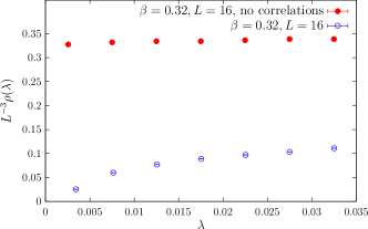
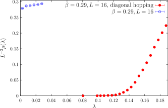
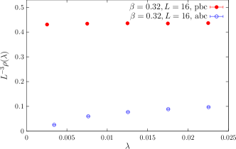
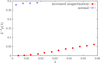
Figure 2: Spectral density in tweaked versions of the toy model: $\hat{\beta}=0$ (top left), TM-diagonal hopping terms (top right), temporal PBC (bottom left), and increased unperturbed eigenvalues (bottom right).

For our numerical investigation we have employed the minimal version of this toy model with only two colours and two time-slices, $N_{c}=N_{T}=2$. In this case there is a single relevant phase, $\phi_{\vec{x}}=\phi^{1}_{\vec{x}}=-\phi^{2}_{\vec{x}}$, and only one relevant Matsubara frequency $\omega(\vec{x})=\frac{\phi_{\vec{x}}+\pi}{2}$, and the “unperturbed” eigenvalues are simply $\pm\eta_{4}(\vec{x})\cos\frac{\phi_{\vec{x}}}{2}$. Since we are interested mainly in the dependence on $\beta$, i.e., on the ordering of the spin system, we fixed $h=1.0$, which leads to a critical $\beta_{c}\approx 0.3$, separating the disordered ($\beta<\beta_{c}$) and ordered ($\beta>\beta_{c}$) phases, corresponding to the confined and deconfined phases of a gauge theory. The “gauge coupling” was also fixed to $\hat{\beta}=5.0$. We then studied the localisation properties of the low modes, and “chiral symmetry breaking”, defined here as the presence of a nonzero spectral density at the origin.

In Fig. 1, left panel, we show the spectral density at the low end of the spectrum, both in the disordered and in the ordered phases. While in the disordered phase one has a nonvanishing $\rho(0)$ and so “chiral symmetry breaking”, in the ordered phase $\rho(0)=0$ and “chiral symmetry” is restored. In order to detect localisation of the eigenmodes we have exploited the fact that delocalised modes obey RMT statistics, while localised modes obey Poisson statistics. We have then computed the integrated probability density $I_{0.5}$ of the unfolded level spacings $s_{i}$, $I_{0.5}=\int_{0}^{0.5}ds\,P_{\lambda}(s)$, with $s_{i}=\frac{\lambda_{i+1}-\lambda_{i}}{\langle\lambda_{i+1}-\lambda_{i}\rangle_{\lambda}}$. Here $P_{\lambda}(s)$ is the probability density of $s$ computed locally in the spectrum in a small interval around $\lambda$. Our results are shown in Fig. 1, right panel, together with the predictions of Poisson statistics and of the appropriate ensemble of RMT, which in the case at hand is the Gaussian Symplectic Ensemble. The transition from Poisson to RMT statistics is evident, and becomes sharper as the volume of the system is increased, thus signaling the presence of a phase transition in the thermodynamic limit. The mobility edge is determined by the crossing point of the curves corresponding to different volumes, and increases as the ordering of the spins increases.

Our minimal toy model is thus able to reproduce the qualitative features of QCD regarding chiral symmetry and localisation. By tweaking the toy model one can further check the relative importance of the two effects caused by ordering, i.e., the decreased density of low unperturbed modes and the decreased mixing of the wave function’s TM components. The same consequences are expected to be observed in QCD. In Fig. 2 we show the spectral density obtained in several modifications of the toy model. In the top left panel, correlations across time-slices are removed by setting $\hat{\beta}=0$, in the ordered phase of the spin model: as a result, chiral symmetry gets broken. In the top right panel, the mixing between TM components is removed by making the hopping terms diagonal in TM, in the disordered phase: this restores chiral symmetry. In the bottom left panel, boundary conditions in the temporal direction are switched from antiperiodic to periodic, in the ordered phase, so increasing the density of low unperturbed modes: chiral symmetry is broken. Finally, in the bottom right panel we artificially increase the unperturbed eigenvalues, in the disordered phase: chiral symmetry is restored. In all cases, chiral symmetry restoration/breaking is accompanied by localisation/delocalisation of the low modes. In conclusion, both mixing of different TM components of the quark wave function (or lack thereof) and the density of low unperturbed modes are crucial for the fate of chiral symmetry and localisation.

4 Conclusions

Recasting the staggered Dirac operator in the form of an Anderson-like Hamiltonian clarifies the relation between the localisation/delocalisation transitions in QCD and in the unitary Anderson model. Moreover, it allows a better understanding of the localisation mechanism at high temperature, and sheds some light on mode delocalisation and on the formation of a chiral condensate via accumulation of small eigenmodes at low temperature. The fate of localisation and chiral symmetry seems to be determined by the ordering of the Polyakov lines, and thus ultimately by the confining properties of the theory. Further work is certainly needed along these lines.

References

- [1] S. Borsányi, G. Endrődi, Z. Fodor, A. Jakovác, S. D. Katz, S. Krieg, C. Ratti and K. K. Szabó, 110772010 [arXiv:1007.2580 [hep-lat]].
- [2] P. de Forcrand and O. Philipsen, 110122008 [arXiv:0808.1096 [hep-lat]].
- [3] F. Karsch and M. Lütgemeier, Nucl. Phys. B 550 (1999) 449 [hep-lat/9812023].
- [4] A. M. García-García and J. C. Osborn, Phys. Rev. D 75 (2007) 034503 [hep-lat/0611019].
- [5] T. G. Kovács, Phys. Rev. Lett. 104 (2010) 031601 [arXiv:0906.5373 [hep-lat]].
- [6] T. G. Kovács and F. Pittler, Phys. Rev. Lett. 105 (2010) 192001 [arXiv:1006.1205 [hep-lat]].
- [7] F. Bruckmann, T. G. Kovács and S. Schierenberg, Phys. Rev. D 84 (2011) 034505 [arXiv:1105.5336 [hep-lat]].
- [8] T. G. Kovács and F. Pittler, Phys. Rev. D 86 (2012) 114515 [arXiv:1208.3475 [hep-lat]].
- [9] M. Giordano, T. G. Kovács and F. Pittler, Phys. Rev. Lett. 112 (2014) 102002 [arXiv:1312.1179 [hep-lat]].
- [10] L. Ujfalusi, M. Giordano, F. Pittler, T. G. Kovács and I. Varga, Phys. Rev. D 92 (2015) 094513 [arXiv:1507.02162 [cond-mat.dis-nn]].
- [11] G. Cossu and S. Hashimoto, (2016) 056 [arXiv:1604.00768 [hep-lat]].
- [12] J. J. M. Verbaarschot and T. Wettig, Ann. Rev. Nucl. Part. Sci. 50 (2000) 343 [hep-ph/0003017].
- [13] M. Giordano, T. G. Kovács, S. D. Katz and F. Pittler, PoS LATTICE 2014 (2014) 214 [arXiv:1410.8392 [hep-lat]].
- [14] P. W. Anderson, Phys. Rev. 109 (1958) 1492.
- [15] K. Slevin and T. Ohtsuki, Phys. Rev. Lett. 78 (1997) 4083 [cond-mat/9704192 [cond-mat.dis-nn]].
- [16] L. Ujfalusi and I. Varga, Phys. Rev. B 91 (2015) 184206 [arXiv:1501.02147 [cond-mat.dis-nn]].
- [17] M. Giordano, T. G. Kovács and F. Pittler, 041122015 [arXiv:1502.02532 [hep-lat]].
- [18] M. Giordano, T. G. Kovács and F. Pittler, 060072016 [arXiv:1603.09548 [hep-lat]].