Weyl semimetal with a boundary at z = 0 𝑧 0 z=0
D. Schmeltzer
Physics Department, City College of the City University of New York,
New York, New York 10031, USA
Abstract
We consider a Weyl semimetals Hamiltonian with two nodes and derive the scattering Hamiltonian in the presence of a boundary at z = 0 𝑧 0 z=0
Weyl fermions represent a pair of particles with opposite chirality described by the massless solution of the Dirac equation Weyl ( 3 D ) 3 𝐷 (3D) Vishwanath ; Xu ( W S M s ) 𝑊 𝑆 𝑀 𝑠 (WSMs) W S M s 𝑊 𝑆 𝑀 𝑠 WSMs Ninomya W S M s 𝑊 𝑆 𝑀 𝑠 WSMs W S M s 𝑊 𝑆 𝑀 𝑠 WSMs Son W S M s 𝑊 𝑆 𝑀 𝑠 WSMs Vishwanath T a A s 𝑇 𝑎 𝐴 𝑠 TaAs T a P 𝑇 𝑎 𝑃 TaP N b A s 𝑁 𝑏 𝐴 𝑠 NbAs N b P 𝑁 𝑏 𝑃 NbP W S M s 𝑊 𝑆 𝑀 𝑠 WSMs 12 12 12 Science
The hallmarks of the W S M s 𝑊 𝑆 𝑀 𝑠 WSMs Science Stern
It is an important task for theory to compute compute the photoemission spectrum for the W S M s 𝑊 𝑆 𝑀 𝑠 WSMs z = 0 𝑧 0 z=0 σ → ⋅ A → ⋅ → 𝜎 → 𝐴 \vec{\sigma}\cdot\vec{A} A → ⋅ p → ⋅ → 𝐴 → 𝑝 \vec{A}\cdot\vec{p} σ → ⋅ A → ⋅ → 𝜎 → 𝐴 \vec{\sigma}\cdot\vec{A}
For the Weyl fermions we consider a Hamiltonian which respects time reversal symmetry and has a broken inversion symmetry.
We consider a simplified model with a single pair of Weyl nodes .
h ( k → ) = τ 3 ( σ 2 k 2 + σ 3 k 3 ) + τ 2 σ 2 g ( k 1 2 − M 2 ) = γ 0 [ γ 3 k 3 + γ 2 k 2 + i σ 2 τ 3 g ( k 1 2 − M 2 ) ] ℎ → 𝑘 subscript 𝜏 3 subscript 𝜎 2 subscript 𝑘 2 subscript 𝜎 3 subscript 𝑘 3 subscript 𝜏 2 subscript 𝜎 2 𝑔 subscript superscript 𝑘 2 1 superscript 𝑀 2 subscript 𝛾 0 delimited-[] subscript 𝛾 3 subscript 𝑘 3 subscript 𝛾 2 subscript 𝑘 2 𝑖 subscript 𝜎 2 subscript 𝜏 3 𝑔 subscript superscript 𝑘 2 1 superscript 𝑀 2 h(\vec{k})=\tau_{3}(\sigma_{2}k_{2}+\sigma_{3}k_{3})+\tau_{2}\sigma_{2}g(k^{2}_{1}-M^{2})=\gamma_{0}\Big{[}\gamma_{3}k_{3}+\gamma_{2}k_{2}+i\sigma_{2}\tau_{3}g(k^{2}_{1}-M^{2})\Big{]} (1)
The matrices σ → → 𝜎 \vec{\sigma} τ → → 𝜏 \vec{\tau} γ 𝛾 \gamma γ 0 subscript 𝛾 0 \gamma_{0} γ i subscript 𝛾 𝑖 \gamma_{i} i = 0 , 1 , 2 , 3 𝑖 0 1 2 3
i=0,1,2,3 γ → = σ → ⊗ i τ 2 → 𝛾 tensor-product → 𝜎 𝑖 subscript 𝜏 2 \vec{\gamma}=\vec{\sigma}\otimes i\tau_{2} γ 5 subscript 𝛾 5 \gamma_{5} γ 5 = i γ 0 γ 1 γ 2 γ 3 subscript 𝛾 5 𝑖 subscript 𝛾 0 subscript 𝛾 1 subscript 𝛾 2 subscript 𝛾 3 \gamma_{5}=i\gamma_{0}\gamma_{1}\gamma_{2}\gamma_{3} g ( k 1 2 − M 2 ) 𝑔 subscript superscript 𝑘 2 1 superscript 𝑀 2 g(k^{2}_{1}-M^{2}) k → = [ k 1 = ± M , k 2 = 0 , k 3 = 0 ] → 𝑘 delimited-[] formulae-sequence subscript 𝑘 1 plus-or-minus 𝑀 formulae-sequence subscript 𝑘 2 0 subscript 𝑘 3 0 \vec{k}=\Big{[}k_{1}=\pm M,k_{2}=0,k_{3}=0\Big{]} L ≤ z ≤ 0 𝐿 𝑧 0 L\leq z\leq 0 z = 0 𝑧 0 z=0 Ψ Ψ \Psi ( 1 ) 1 (1) z 𝑧 z z 𝑧 z γ 3 = σ 3 ⊗ i τ 2 subscript 𝛾 3 tensor-product subscript 𝜎 3 𝑖 subscript 𝜏 2 \gamma_{3}=\sigma_{3}\otimes i\tau_{2} γ 3 Ψ = ± Ψ subscript 𝛾 3 Ψ plus-or-minus Ψ \gamma_{3}\Psi=\pm\Psi
γ 0 [ ( − i ∂ z + i σ 2 g ( k 1 2 − M 2 ) τ 3 ] Ψ = [ E − σ 2 k 2 τ 3 ] Ψ ; Ψ = [ Ψ 1 , Ψ 2 ] T \gamma_{0}\Big{[}(-i\partial_{z}+i\sigma_{2}g(k^{2}_{1}-M^{2})\tau_{3}\Big{]}\Psi=\Big{[}E-\sigma_{2}k_{2}\tau_{3}\Big{]}\Psi;\hskip 7.22743pt\Psi=\Big{[}\Psi_{1},\Psi_{2}\Big{]}^{T} (2)
The right hand side of gives us two equations, [ E − σ 2 k 2 ] Ψ 1 = 0 delimited-[] 𝐸 subscript 𝜎 2 subscript 𝑘 2 subscript Ψ 1 0 \Big{[}E-\sigma_{2}k_{2}\Big{]}\Psi_{1}=0 [ E + σ 2 k 2 ] Ψ 2 = 0 delimited-[] 𝐸 subscript 𝜎 2 subscript 𝑘 2 subscript Ψ 2 0 \Big{[}E+\sigma_{2}k_{2}\Big{]}\Psi_{2}=0 z = 0 𝑧 0 z=0 σ 2 Ψ 1 , s = 1 2 = Ψ 1 , s = 1 2 subscript 𝜎 2 subscript Ψ 1 𝑠
1 2 subscript Ψ 1 𝑠
1 2 \sigma_{2}\Psi_{1,s=\frac{1}{2}}=\Psi_{1,s=\frac{1}{2}} σ 2 Ψ 2 , s = − 1 2 = − Ψ 2 , s = − 1 2 subscript 𝜎 2 subscript Ψ 2 𝑠
1 2 subscript Ψ 2 𝑠
1 2 \sigma_{2}\Psi_{2,s=-\frac{1}{2}}=-\Psi_{2,s=-\frac{1}{2}} E 1 , s = 1 2 = k 2 subscript 𝐸 1 𝑠
1 2 subscript 𝑘 2 E_{1,s=\frac{1}{2}}=k_{2} E 1 , s = − 1 2 = − k 2 subscript 𝐸 1 𝑠
1 2 subscript 𝑘 2 E_{1,s=-\frac{1}{2}}=-k_{2} σ 2 Ψ 2 , s = 1 2 = Ψ 2 , s = 1 2 subscript 𝜎 2 subscript Ψ 2 𝑠
1 2 subscript Ψ 2 𝑠
1 2 \sigma_{2}\Psi_{2,s=\frac{1}{2}}=\Psi_{2,s=\frac{1}{2}} σ 2 Ψ 2 , s = − 1 2 = − Ψ 2 , s = − 1 2 subscript 𝜎 2 subscript Ψ 2 𝑠
1 2 subscript Ψ 2 𝑠
1 2 \sigma_{2}\Psi_{2,s=-\frac{1}{2}}=-\Psi_{2,s=-\frac{1}{2}} E 2 , s = 1 2 = − k 2 subscript 𝐸 2 𝑠
1 2 subscript 𝑘 2 E_{2,s=\frac{1}{2}}=-k_{2} E 2 , s = − 1 2 = k 2 subscript 𝐸 2 𝑠
1 2 subscript 𝑘 2 E_{2,s=-\frac{1}{2}}=k_{2} C ^ 1 ( k 1 , k 2 , z ) subscript ^ 𝐶 1 subscript 𝑘 1 subscript 𝑘 2 𝑧 \hat{C}_{1}(k_{1},k_{2},z) C ^ 2 ( k 1 , k 2 , z ) subscript ^ 𝐶 2 subscript 𝑘 1 subscript 𝑘 2 𝑧 \hat{C}_{2}(k_{1},k_{2},z) Ψ 1 , s = ± 1 2 ( σ ; k 1 , k 2 , z ) subscript Ψ 1 𝑠
plus-or-minus 1 2 𝜎 subscript 𝑘 1 subscript 𝑘 2 𝑧
\Psi_{1,s=\pm\frac{1}{2}}(\sigma;k_{1},k_{2},z) Ψ 2 , s = ± 1 2 ( σ ; k 1 , k 2 , z ) subscript Ψ 2 𝑠
plus-or-minus 1 2 𝜎 subscript 𝑘 1 subscript 𝑘 2 𝑧
\Psi_{2,s=\pm\frac{1}{2}}(\sigma;k_{1},k_{2},z) k → ∥ = [ k 1 , k 2 ] subscript → 𝑘 parallel-to subscript 𝑘 1 subscript 𝑘 2 \vec{k}_{\parallel}=\Big{[}k_{1},k_{2}\Big{]}
1 2 ( Ψ 1 , s = − 1 2 ( σ ; k 1 , k 2 , z ) + Ψ 2 , s = − 1 2 ( σ ; k 1 , k 2 , z ) ) = η s = 1 2 ( σ ) C ^ 1 ( k 1 , k 2 , z ) 1 2 subscript Ψ 1 𝑠
1 2 𝜎 subscript 𝑘 1 subscript 𝑘 2 𝑧
subscript Ψ 2 𝑠
1 2 𝜎 subscript 𝑘 1 subscript 𝑘 2 𝑧
subscript 𝜂 𝑠 1 2 𝜎 subscript ^ 𝐶 1 subscript 𝑘 1 subscript 𝑘 2 𝑧 \displaystyle\frac{1}{\sqrt{2}}\Big{(}\Psi_{1,s=-\frac{1}{2}}(\sigma;k_{1},k_{2},z)+\Psi_{2,s=-\frac{1}{2}}(\sigma;k_{1},k_{2},z)\Big{)}=\eta_{s=\frac{1}{2}}(\sigma)\hat{C}_{1}(k_{1},k_{2},z)
1 2 ( Ψ 1 , s = − 1 2 ( σ ; k 1 , k 2 , z ) + Ψ 2 , s = 1 2 ( σ ; k 1 , k 2 , z ) ) = η s = − 1 2 ( σ ) C ^ 2 ( k 1 , k 2 , z ) 1 2 subscript Ψ 1 𝑠
1 2 𝜎 subscript 𝑘 1 subscript 𝑘 2 𝑧
subscript Ψ 2 𝑠
1 2 𝜎 subscript 𝑘 1 subscript 𝑘 2 𝑧
subscript 𝜂 𝑠 1 2 𝜎 subscript ^ 𝐶 2 subscript 𝑘 1 subscript 𝑘 2 𝑧 \displaystyle\frac{1}{\sqrt{2}}\Big{(}\Psi_{1,s=-\frac{1}{2}}(\sigma;k_{1},k_{2},z)+\Psi_{2,s=\frac{1}{2}}(\sigma;k_{1},k_{2},z)\Big{)}=\eta_{s=-\frac{1}{2}}(\sigma)\hat{C}_{2}(k_{1},k_{2},z)
Where η s = 1 2 = 1 2 [ 1 , − i ] T subscript 𝜂 𝑠 1 2 1 2 superscript 1 𝑖 𝑇 \eta_{s=\frac{1}{2}}=\frac{1}{\sqrt{2}}\Big{[}1,-i\Big{]}^{T} η s = − 1 2 = 1 2 [ 1 , i ] T subscript 𝜂 𝑠 1 2 1 2 superscript 1 𝑖 𝑇 \eta_{s=-\frac{1}{2}}=\frac{1}{\sqrt{2}}\Big{[}1,i\Big{]}^{T} σ 2 η s = ± 1 2 = ± η s = ± 1 2 subscript 𝜎 2 subscript 𝜂 𝑠 plus-or-minus 1 2 plus-or-minus subscript 𝜂 𝑠 plus-or-minus 1 2 \sigma_{2}\eta_{s=\pm\frac{1}{2}}=\pm\eta_{s=\pm\frac{1}{2}} D 1 subscript 𝐷 1 D_{1} D 2 subscript 𝐷 2 D_{2}
The spinors C ^ 1 ( k 1 , k 2 , z ) subscript ^ 𝐶 1 subscript 𝑘 1 subscript 𝑘 2 𝑧 \hat{C}_{1}(k_{1},k_{2},z) C ^ 2 ( k 1 , k 2 , z ) subscript ^ 𝐶 2 subscript 𝑘 1 subscript 𝑘 2 𝑧 \hat{C}_{2}(k_{1},k_{2},z)
[ − ∂ z + g ( k 1 2 − M 2 ) ] C ^ 1 ( k 1 , k 2 , z ) = 0 delimited-[] subscript 𝑧 𝑔 subscript superscript 𝑘 2 1 superscript 𝑀 2 subscript ^ 𝐶 1 subscript 𝑘 1 subscript 𝑘 2 𝑧 0 \displaystyle\Big{[}-\partial_{z}+g(k^{2}_{1}-M^{2})\Big{]}\hat{C}_{1}(k_{1},k_{2},z)=0
[ − ∂ z − g ( k 1 2 − M 2 ) ] C ^ 2 ( k 1 , k 2 , z ) = 0 delimited-[] subscript 𝑧 𝑔 subscript superscript 𝑘 2 1 superscript 𝑀 2 subscript ^ 𝐶 2 subscript 𝑘 1 subscript 𝑘 2 𝑧 0 \displaystyle\Big{[}-\partial_{z}-g(k^{2}_{1}-M^{2})\Big{]}\hat{C}_{2}(k_{1},k_{2},z)=0
The solution of equation ( 4 ) 4 (4) C 1 ( k 1 , k 2 ) subscript 𝐶 1 subscript 𝑘 1 subscript 𝑘 2 C_{1}(k_{1},k_{2}) C 2 ( k 1 , k 2 ) subscript 𝐶 2 subscript 𝑘 1 subscript 𝑘 2 C_{2}(k_{1},k_{2})
C ^ 1 ( k 1 , k 2 , z ) = θ [ − z ] θ [ k 1 2 − M 2 ] 2 g M 2 ( ( k 1 / M ) 2 − 1 ) e g M 2 ( ( k 1 / M ) 2 − 1 ) z C 1 ( k 1 , k 2 ) subscript ^ 𝐶 1 subscript 𝑘 1 subscript 𝑘 2 𝑧 𝜃 delimited-[] 𝑧 𝜃 delimited-[] subscript superscript 𝑘 2 1 superscript 𝑀 2 2 𝑔 superscript 𝑀 2 superscript subscript 𝑘 1 𝑀 2 1 superscript 𝑒 𝑔 superscript 𝑀 2 superscript subscript 𝑘 1 𝑀 2 1 𝑧 subscript 𝐶 1 subscript 𝑘 1 subscript 𝑘 2 \displaystyle\hat{C}_{1}(k_{1},k_{2},z)=\theta[-z]\theta[k^{2}_{1}-M^{2}]\sqrt{2gM^{2}((k_{1}/M)^{2}-1)}e^{gM^{2}((k_{1}/M)^{2}-1)z}C_{1}(k_{1},k_{2})
C ^ 2 ( k 1 , k 2 , z ) = θ [ − z ] θ [ − k 1 2 + M 2 ] 2 g M 2 ( − ( k 1 / M ) 2 + 1 ) e g M 2 ( − ( k 1 / M ) 2 + 1 ) z C 1 ( k 1 , k 2 ) subscript ^ 𝐶 2 subscript 𝑘 1 subscript 𝑘 2 𝑧 𝜃 delimited-[] 𝑧 𝜃 delimited-[] subscript superscript 𝑘 2 1 superscript 𝑀 2 2 𝑔 superscript 𝑀 2 superscript subscript 𝑘 1 𝑀 2 1 superscript 𝑒 𝑔 superscript 𝑀 2 superscript subscript 𝑘 1 𝑀 2 1 𝑧 subscript 𝐶 1 subscript 𝑘 1 subscript 𝑘 2 \displaystyle\hat{C}_{2}(k_{1},k_{2},z)=\theta[-z]\theta[-k^{2}_{1}+M^{2}]\sqrt{2gM^{2}(-(k_{1}/M)^{2}+1)}e^{gM^{2}(-(k_{1}/M)^{2}+1)z}C_{1}(k_{1},k_{2})
Where θ [ − z ] 𝜃 delimited-[] 𝑧 \theta[-z] z ≤ 0 𝑧 0 z\leq 0 θ [ k 1 2 − M 2 ] 𝜃 delimited-[] subscript superscript 𝑘 2 1 superscript 𝑀 2 \theta[k^{2}_{1}-M^{2}] θ [ − k 1 2 + M 2 ] 𝜃 delimited-[] subscript superscript 𝑘 2 1 superscript 𝑀 2 \theta[-k^{2}_{1}+M^{2}] μ > 0 𝜇 0 \mu>0
Next we derive the Hamiltonian for the photoemission which in the final form is given in Eq.( 13 ) 13 (13) 𝐇 ( 𝐖 ) superscript 𝐇 𝐖 \mathbf{H^{(W)}} z = 0 𝑧 0 z=0
H ( W ) = ∫ d 2 k ( 2 π ) 2 [ C 1 † ( k 1 , k 2 ) ( k 2 θ [ k 2 ] θ [ k 1 2 − M 2 ] ) C 1 ( k 1 , k 2 ) − C 2 † ( k 1 , k 2 ) ( k 2 θ [ − k 2 ] θ [ M 2 − k 1 2 ] ) C 2 ( k 1 , k 2 ) ] superscript 𝐻 𝑊 superscript 𝑑 2 𝑘 superscript 2 𝜋 2 delimited-[] subscript superscript 𝐶 † 1 subscript 𝑘 1 subscript 𝑘 2 subscript 𝑘 2 𝜃 delimited-[] subscript 𝑘 2 𝜃 delimited-[] subscript superscript 𝑘 2 1 superscript 𝑀 2 subscript 𝐶 1 subscript 𝑘 1 subscript 𝑘 2 subscript superscript 𝐶 † 2 subscript 𝑘 1 subscript 𝑘 2 subscript 𝑘 2 𝜃 delimited-[] subscript 𝑘 2 𝜃 delimited-[] superscript 𝑀 2 subscript superscript 𝑘 2 1 subscript 𝐶 2 subscript 𝑘 1 subscript 𝑘 2 H^{(W)}=\int\frac{d^{2}k}{(2\pi)^{2}}\Big{[}C^{\dagger}_{1}(k_{1},k_{2})\Big{(}k_{2}\theta[k_{2}]\theta[k^{2}_{1}-M^{2}]\Big{)}C_{1}(k_{1},k_{2})-C^{\dagger}_{2}(k_{1},k_{2})\Big{(}k_{2}\theta[-k_{2}]\theta[M^{2}-k^{2}_{1}]\Big{)}C_{2}(k_{1},k_{2})\Big{]} (6)
θ [ k 2 ] 𝜃 delimited-[] subscript 𝑘 2 \theta[k_{2}] k 2 > 0 subscript 𝑘 2 0 k_{2}>0 𝐟 σ ( 𝐤 𝟏 , 𝐤 𝟐 , 𝐳 > 𝟎 ) subscript 𝐟 𝜎 subscript 𝐤 1 subscript 𝐤 2 𝐳
0 \mathbf{f_{\sigma}(k_{1},k_{2},z>0)} f σ ( k 1 , k 2 , z > 0 ) = ∫ 0 Λ d k z 2 π e i k z z f σ ( k 1 , s k 2 , k z ) subscript 𝑓 𝜎 subscript 𝑘 1 subscript 𝑘 2 𝑧
0 superscript subscript 0 Λ 𝑑 subscript 𝑘 𝑧 2 𝜋 superscript 𝑒 𝑖 subscript 𝑘 𝑧 𝑧 subscript 𝑓 𝜎 subscript 𝑘 1 𝑠 subscript 𝑘 2 subscript 𝑘 𝑧 f_{\sigma}(k_{1},k_{2},z>0)=\int_{0}^{\Lambda}\frac{dk_{z}}{2\pi}e^{ik_{z}z}f_{\sigma}(k_{1},sk_{2},k_{z}) t ( k z ) 𝑡 subscript 𝑘 𝑧 t(k_{z}) 1 L e i k z z 1 𝐿 superscript 𝑒 𝑖 subscript 𝑘 𝑧 𝑧 \frac{1}{\sqrt{L}}e^{ik_{z}z} 2 g M 2 | ( k 1 / M ) 2 − 1 | e g M 2 | ( k 1 / M ) 2 − 1 | z 2 𝑔 superscript 𝑀 2 superscript subscript 𝑘 1 𝑀 2 1 superscript 𝑒 𝑔 superscript 𝑀 2 superscript subscript 𝑘 1 𝑀 2 1 𝑧 \sqrt{2gM^{2}|(k_{1}/M)^{2}-1|}e^{gM^{2}|(k_{1}/M)^{2}-1|z} [ − d , 0 ] 𝑑 0 [-d,0] TopI t ( k z ) 𝑡 subscript 𝑘 𝑧 t(k_{z}) g ^ ^ 𝑔 \hat{g} d 𝑑 d
t ( k z ) = ∫ − d 0 𝑑 z 2 g M 2 | ( k 1 / M ) 2 − 1 | e g M 2 | ( k 1 / M ) 2 − 1 | z 1 L e i k z z 𝑡 subscript 𝑘 𝑧 superscript subscript 𝑑 0 differential-d 𝑧 2 𝑔 superscript 𝑀 2 superscript subscript 𝑘 1 𝑀 2 1 superscript 𝑒 𝑔 superscript 𝑀 2 superscript subscript 𝑘 1 𝑀 2 1 𝑧 1 𝐿 superscript 𝑒 𝑖 subscript 𝑘 𝑧 𝑧 \displaystyle t(k_{z})=\int_{-d}^{0}\,dz\sqrt{2gM^{2}|(k_{1}/M)^{2}-1|}e^{gM^{2}|(k_{1}/M)^{2}-1|z}\frac{1}{\sqrt{L}}e^{ik_{z}z}
t ( k z ) t ∗ ( k z ) ≈ ( d L ) 2 g ^ | ( k 1 / M ) 2 − 1 | g ^ [ ( k 1 / M ) 2 − 1 ] 2 + ( k z d ) 2 ; g M 2 = g ^ d − 1 formulae-sequence 𝑡 subscript 𝑘 𝑧 superscript 𝑡 subscript 𝑘 𝑧 𝑑 𝐿 2 ^ 𝑔 superscript subscript 𝑘 1 𝑀 2 1 ^ 𝑔 superscript delimited-[] superscript subscript 𝑘 1 𝑀 2 1 2 superscript subscript 𝑘 𝑧 𝑑 2 𝑔 superscript 𝑀 2 ^ 𝑔 superscript 𝑑 1 \displaystyle t(k_{z})t^{*}(k_{z})\approx(\frac{d}{L})\frac{2\hat{g}|(k_{1}/M)^{2}-1|}{\hat{g}[(k_{1}/M)^{2}-1]^{2}+(k_{z}d)^{2}};gM^{2}=\hat{g}d^{-1}
This term is essential for the photoemission process. The Weyl electrons couples light through the Dirac form σ → ⋅ A → ⋅ → 𝜎 → 𝐴 \vec{\sigma}\cdot\vec{A} z > 0 𝑧 0 z>0 A → ⋅ p → ⋅ → 𝐴 → 𝑝 \vec{A}\cdot\vec{p} p → → 𝑝 \vec{p} σ 2 τ 2 g ( k 1 2 − M 2 ) subscript 𝜎 2 subscript 𝜏 2 𝑔 subscript superscript 𝑘 2 1 superscript 𝑀 2 \sigma_{2}\tau_{2}g(k^{2}_{1}-M^{2}) k 1 2 ≠ M 2 subscript superscript 𝑘 2 1 superscript 𝑀 2 k^{2}_{1}\neq M^{2} ( 1 ) 1 (1) W e y l − V a c u m 𝑊 𝑒 𝑦 𝑙 𝑉 𝑎 𝑐 𝑢 𝑚 Weyl-Vacum 𝐇 ( 𝐖 , 𝐕 ) superscript 𝐇 𝐖 𝐕 \mathbf{H^{(W,V)}}
H ( W , V ) = ∑ σ = ↑ , ↓ ∫ d 2 k ( 2 π ) 2 ∫ 0 Λ d k z 2 π [ t ( k z ) ( τ + ( k 1 ) θ [ k 2 ] C 1 † ( k 1 , k 2 ) η s = 1 2 ( σ ) f σ ( k 1 , k 2 , k z ) \displaystyle H^{(W,V)}=\sum_{\sigma=\uparrow,\downarrow}\int\frac{d^{2}k}{(2\pi)^{2}}\int_{0}^{\Lambda}\frac{dk_{z}}{2\pi}\Big{[}t(k_{z})\Big{(}\tau_{+}(k_{1})\theta[k_{2}]C^{\dagger}_{1}(k_{1},k_{2})\eta_{s=\frac{1}{2}}(\sigma)f_{\sigma}(k_{1},k_{2},k_{z})
+ τ − ( k 1 ) θ [ − k 2 ] C 2 † ( k 1 , k 2 ) η s = − 1 2 ( σ ) f σ ( k 1 , k 2 , k z ) ) + h . c . ] \displaystyle+\tau_{-}(k_{1})\theta[-k_{2}]C^{\dagger}_{2}(k_{1},k_{2})\eta_{s=-\frac{1}{2}}(\sigma)f_{\sigma}(k_{1},k_{2},k_{z})\Big{)}+h.c.\Big{]}
τ + ( k 1 ) = θ [ k 1 2 − M 2 ] , τ − ( k 1 ) = θ [ M 2 − k 1 2 ] ; formulae-sequence subscript 𝜏 subscript 𝑘 1 𝜃 delimited-[] subscript superscript 𝑘 2 1 superscript 𝑀 2 subscript 𝜏 subscript 𝑘 1 𝜃 delimited-[] superscript 𝑀 2 subscript superscript 𝑘 2 1 \displaystyle\tau_{+}(k_{1})=\theta[k^{2}_{1}-M^{2}],\tau_{-}(k_{1})=\theta[M^{2}-k^{2}_{1}];
In the photoemission process the momentum parallel to the surface is conserved k → | | = [ k 1 , k 2 ] \vec{k}_{||}=\Big{[}k_{1},k_{2}\Big{]} E ( V ) = ϵ ( W ) + W superscript 𝐸 𝑉 superscript italic-ϵ 𝑊 𝑊 E^{(V)}=\epsilon^{(W)}+W ϵ ( W ) superscript italic-ϵ 𝑊 \epsilon^{(W)} W 𝑊 W Ω Ω \Omega ϵ ( W ) + ℏ Ω superscript italic-ϵ 𝑊 Planck-constant-over-2-pi Ω \epsilon^{(W)}+\hbar\Omega E ( V ) = ϵ ( W ) + W + ℏ Ω superscript 𝐸 𝑉 superscript italic-ϵ 𝑊 𝑊 Planck-constant-over-2-pi Ω E^{(V)}=\epsilon^{(W)}+W+\hbar\Omega k z subscript 𝑘 𝑧 k_{z} Eastman
k z = 2 m ℏ 2 [ ( ϵ ( W ) + ℏ Ω ) cos 2 ( θ ) − W ] , ϵ ( W ) = k 2 θ [ k 2 ] + ( − k 2 ) θ [ − k 2 ] formulae-sequence subscript 𝑘 𝑧 2 𝑚 superscript Planck-constant-over-2-pi 2 delimited-[] superscript italic-ϵ 𝑊 Planck-constant-over-2-pi Ω superscript 2 𝜃 𝑊 superscript italic-ϵ 𝑊 subscript 𝑘 2 𝜃 delimited-[] subscript 𝑘 2 subscript 𝑘 2 𝜃 delimited-[] subscript 𝑘 2 k_{z}=\sqrt{\frac{2m}{\hbar^{2}}\Big{[}\Big{(}\epsilon^{(W)}+\hbar\Omega\Big{)}\cos^{2}(\theta)-W\Big{]}},\epsilon^{(W)}=k_{2}\theta[k_{2}]+(-k_{2})\theta[-k_{2}] (9)
For cos 2 ( θ ) ≈ 1 superscript 2 𝜃 1 \cos^{2}(\theta)\approx 1 k z = 2 m ℏ 2 [ ϵ ( W ) + ℏ Ω − W ] subscript 𝑘 𝑧 2 𝑚 superscript Planck-constant-over-2-pi 2 delimited-[] superscript italic-ϵ 𝑊 Planck-constant-over-2-pi Ω 𝑊 k_{z}=\sqrt{\frac{2m}{\hbar^{2}}\Big{[}\epsilon^{(W)}+\hbar\Omega-W\Big{]}}
The Hamilonian for the free electrons is a function of the conserved parallel momentum 𝐇 ( 𝐕 ) superscript 𝐇 𝐕 \mathbf{H^{(V)}}
H ( V ) = ∫ d 2 k ( 2 π ) 2 ∑ σ [ f σ † ( k → ) ( k 2 θ [ k 2 ] + W ) θ [ k 1 2 − M 2 ] f σ ( k → ) + f σ † ( k → ) ( ( − k 2 ) θ [ − k 2 ] + W ) θ [ − k 1 2 + M 2 ] f σ ( k → ) ] superscript 𝐻 𝑉 superscript 𝑑 2 𝑘 superscript 2 𝜋 2 subscript 𝜎 delimited-[] subscript superscript 𝑓 † 𝜎 → 𝑘 subscript 𝑘 2 𝜃 delimited-[] subscript 𝑘 2 𝑊 𝜃 delimited-[] subscript superscript 𝑘 2 1 superscript 𝑀 2 subscript 𝑓 𝜎 → 𝑘 subscript superscript 𝑓 † 𝜎 → 𝑘 subscript 𝑘 2 𝜃 delimited-[] subscript 𝑘 2 𝑊 𝜃 delimited-[] subscript superscript 𝑘 2 1 superscript 𝑀 2 subscript 𝑓 𝜎 → 𝑘 H^{(V)}=\int\frac{d^{2}k}{(2\pi)^{2}}\sum_{\sigma}\Big{[}f^{\dagger}_{\sigma}(\vec{k})\Big{(}k_{2}\theta[k_{2}]+W\Big{)}\theta[k^{2}_{1}-M^{2}]f_{\sigma}(\vec{k})+f^{\dagger}_{\sigma}(\vec{k})\Big{(}(-k_{2})\theta[-k_{2}]+W\Big{)}\theta[-k^{2}_{1}+M^{2}]f_{\sigma}(\vec{k})\Big{]} (10)
Next we consider the coupling of the photon to the surface electrons. The boundary at z = 0 𝑧 0 z=0 s p i n o r 𝑠 𝑝 𝑖 𝑛 𝑜 𝑟 spinor η s ( σ ) subscript 𝜂 𝑠 𝜎 \eta_{s}(\sigma) y 𝑦 y L ≤ z ≤ 0 𝐿 𝑧 0 L\leq z\leq 0 Ω Ω \Omega k z = Ω c ⋅ c o s ( θ ) subscript 𝑘 𝑧 Ω ⋅ 𝑐 𝑐 𝑜 𝑠 𝜃 k_{z}=\frac{\Omega}{c\cdot cos(\theta)} σ → ⋅ A → ⋅ → 𝜎 → 𝐴 \vec{\sigma}\cdot\vec{A} 𝐇 ( 𝐞𝐱𝐭 ) superscript 𝐇 𝐞𝐱𝐭 \mathbf{H^{(ext)}}
H ( e x t ) = ℏ 2 ϵ ¯ Ω ∑ α = 1 , 2 ∫ d 2 k ( 2 π ) 2 ∫ − L 0 d z [ 2 g ( k 1 2 − M 2 ) e 2 g M 2 ( k 1 2 − M 2 ) z τ + ( k 1 ) C 1 † ( k 1 , k 2 ) C 1 ( k 1 , k 2 ) ( A α e − i Ω t \displaystyle H^{(ext)}=\sqrt{\frac{\hbar}{2\bar{\epsilon}\Omega}}\sum_{\alpha=1,2}\int\frac{d^{2}k}{(2\pi)^{2}}\int_{-L}^{0}\,dz\Big{[}2g(k^{2}_{1}-M^{2})e^{2gM^{2}(k^{2}_{1}-M^{2})z}\tau_{+}(k_{1})C_{1}^{\dagger}(k_{1},k_{2})C_{1}(k_{1},k_{2})(A_{\alpha}e^{-i\Omega t}
e i k z z + A α † e i Ω t e − i k z z ) + 2 g ( − k 1 2 + M 2 ) e 2 g ( − k 1 2 + M 2 ) z τ − ( k 1 ) C 2 † ( k 1 , k 2 ) C 2 ( k 1 , k 2 ) ( A α e − i Ω t e i k z z \displaystyle e^{ik_{z}z}+A^{\dagger}_{\alpha}e^{i\Omega t}e^{-ik_{z}z})+2g(-k^{2}_{1}+M^{2})e^{2g(-k^{2}_{1}+M^{2})z}\tau_{-}(k_{1})C_{2}^{\dagger}(k_{1},k_{2})C_{2}(k_{1},k_{2})(A_{\alpha}e^{-i\Omega t}e^{ik_{z}z}
+ A α † e i Ω t e − i k z z ) ] ∣ k z = Ω c ⋅ c o s ( θ ) 𝐞 𝐲 α ( θ , φ ) \displaystyle+A^{\dagger}_{\alpha}e^{i\Omega t}e^{-ik_{z}z})\Big{]}\mid_{k_{z}=\frac{\Omega}{c\cdot cos(\theta)}}\mathbf{e^{y}_{\alpha}(\theta,\varphi)}
= ℏ 2 ϵ ¯ Ω ∑ α = 1 , 2 ∫ d 2 k ( 2 π ) 2 [ τ + ( k 1 ) C 1 † ( k 1 , k 2 ) C 1 ( k 1 , k 2 ) ( F + ( k 1 , Ω ) A α e − i Ω t + F + ( k 1 , − Ω ) A α † e i Ω t ) \displaystyle=\sqrt{\frac{\hbar}{2\bar{\epsilon}\Omega}}\sum_{\alpha=1,2}\int\frac{d^{2}k}{(2\pi)^{2}}\Big{[}\tau_{+}(k_{1})C_{1}^{\dagger}(k_{1},k_{2})C_{1}(k_{1},k_{2})\Big{(}F_{+}(k_{1},\Omega)A_{\alpha}e^{-i\Omega t}+F_{+}(k_{1},-\Omega)A^{\dagger}_{\alpha}e^{i\Omega t}\Big{)}
+ τ − ( k 1 ) C 2 † ( k 1 , k 2 ) C 2 ( k 1 , k 2 ) ( F − ( k 1 , Ω ) A α e − i Ω t + F − ( k 1 , − Ω ) A α † e i Ω t ) ] 𝐞 𝐲 α ( θ , φ ) \displaystyle+\tau_{-}(k_{1})C_{2}^{\dagger}(k_{1},k_{2})C_{2}(k_{1},k_{2})\Big{(}F_{-}(k_{1},\Omega)A_{\alpha}e^{-i\Omega t}+F_{-}(k_{1},-\Omega)A^{\dagger}_{\alpha}e^{i\Omega t}\Big{)}\Big{]}\mathbf{e^{y}_{\alpha}(\theta,\varphi)}
The representation of the Weyl fermions given in Eq.( 5 ) 5 (5) F + ( k 1 , ± Ω ) subscript 𝐹 subscript 𝑘 1 plus-or-minus Ω F_{+}(k_{1},\pm\Omega) F − ( k 1 , ± Ω ) subscript 𝐹 subscript 𝑘 1 plus-or-minus Ω F_{-}(k_{1},\pm\Omega)
F + ( k 1 , ± Ω ) = 2 g ( k 1 2 − M 2 ) ( 1 − e 2 g ( k 1 2 − M 2 ) L e ± i ( Ω c ⋅ c o s ( θ ) ) L 2 g ( k 1 2 − M 2 ) ± i ( Ω c ⋅ c o s ( θ ) ) ) subscript 𝐹 subscript 𝑘 1 plus-or-minus Ω 2 𝑔 subscript superscript 𝑘 2 1 superscript 𝑀 2 1 superscript 𝑒 2 𝑔 subscript superscript 𝑘 2 1 superscript 𝑀 2 𝐿 superscript 𝑒 plus-or-minus 𝑖 Ω ⋅ 𝑐 𝑐 𝑜 𝑠 𝜃 𝐿 plus-or-minus 2 𝑔 subscript superscript 𝑘 2 1 superscript 𝑀 2 𝑖 Ω ⋅ 𝑐 𝑐 𝑜 𝑠 𝜃 \displaystyle F_{+}(k_{1},\pm\Omega)=2g(k^{2}_{1}-M^{2})\Big{(}\frac{1-e^{2g(k^{2}_{1}-M^{2})L}e^{\pm i(\frac{\Omega}{c\cdot cos(\theta)})L}}{{2g(k^{2}_{1}-M^{2})\pm i(\frac{\Omega}{c\cdot cos(\theta)})}}\Big{)}
F − ( k 1 , ± Ω ) = 2 g ( − k 1 2 + M 2 ) ( 1 − e 2 g ( − k 1 2 + M 2 ) L e ± i ( Ω c ⋅ c o s ( θ ) ) L 2 g ( − k 1 2 + M 2 ) ± i ( Ω c ⋅ c o s ( θ ) ) ) subscript 𝐹 subscript 𝑘 1 plus-or-minus Ω 2 𝑔 subscript superscript 𝑘 2 1 superscript 𝑀 2 1 superscript 𝑒 2 𝑔 subscript superscript 𝑘 2 1 superscript 𝑀 2 𝐿 superscript 𝑒 plus-or-minus 𝑖 Ω ⋅ 𝑐 𝑐 𝑜 𝑠 𝜃 𝐿 plus-or-minus 2 𝑔 subscript superscript 𝑘 2 1 superscript 𝑀 2 𝑖 Ω ⋅ 𝑐 𝑐 𝑜 𝑠 𝜃 \displaystyle F_{-}(k_{1},\pm\Omega)=2g(-k^{2}_{1}+M^{2})\Big{(}\frac{1-e^{2g(-k^{2}_{1}+M^{2})L}e^{\pm i(\frac{\Omega}{c\cdot cos(\theta)})L}}{{2g(-k^{2}_{1}+M^{2})\pm i(\frac{\Omega}{c\cdot cos(\theta)})}}\Big{)}
The y 𝑦 y e α = 1 , 2 y ( θ , ϕ ) subscript superscript 𝑒 𝑦 𝛼 1 2
𝜃 italic-ϕ e^{y}_{\alpha=1,2}(\theta,\phi) TopI α = 1 , 2 𝛼 1 2
\alpha=1,2 p → | p → | = [ sin ( θ ) cos ( ϕ ) , sin ( θ ) sin ( ϕ ) , cos ( θ ) ] → 𝑝 → 𝑝 𝜃 italic-ϕ 𝜃 italic-ϕ 𝜃
\frac{\vec{p}}{|\vec{p}|}=\Big{[}\sin(\theta)\cos(\phi),\sin(\theta)\sin(\phi),\cos(\theta)\Big{]} ϵ ¯ ¯ italic-ϵ \bar{\epsilon} c 𝑐 c | Ω > ket Ω |\Omega> A α | Ω > = 𝐀 α | Ω > subscript 𝐴 𝛼 ket Ω subscript 𝐀 𝛼 ket Ω A_{\alpha}|\Omega>=\mathbf{A_{\alpha}}|\Omega> 𝐀 α subscript 𝐀 𝛼 \mathbf{A_{\alpha}} ( 6 , 8 , 10 , 11 ) 6 8 10 11 (6,8,10,11) 𝐇 𝐇 \mathbf{H}
H = H ( W ) + H ( V ) + H ( W − V ) + H ( e x t . ) H=H^{(W)}+H^{(V)}+H^{(W-V)}+H^{(ext.)} (13)
The spinor structure guaranty that the y 𝑦 y y 𝑦 y S y ( k → , k z ) superscript 𝑆 𝑦 → 𝑘 subscript 𝑘 𝑧 S^{y}(\vec{k},k_{z}) S y ( k → , k z ) superscript 𝑆 𝑦 → 𝑘 subscript 𝑘 𝑧 S^{y}(\vec{k},k_{z}) 𝐆 α , β ( k → , k z ; δ t ) subscript 𝐆 𝛼 𝛽
→ 𝑘 subscript 𝑘 𝑧 𝛿 𝑡 \mathbf{G}_{\alpha,\beta}(\vec{k},k_{z};\delta t) | g ⟩ ket 𝑔 |g\rangle
S y ( k → , k z ) = − i ∑ α = ↑ , ↓ ∑ β = ↑ , ↓ [ σ y ] α , β ∫ d ω 2 π 𝐆 α , β ( K → , k z = 0 ; ω ) i ω δ t \displaystyle S^{y}(\vec{k},k_{z})=-i\sum_{\alpha=\uparrow,\downarrow}\sum_{\beta=\uparrow,\downarrow}\Big{[}\sigma^{y}\Big{]}_{\alpha,\beta}\int\frac{d\omega}{2\pi}\mathbf{G}_{\alpha,\beta}(\vec{K},k_{z}=0;\omega)^{i\omega\delta t}
𝐒 𝐲 ( k → , k z ; ω ) = [ 𝐆 ↓ , ↑ ( k → , k z ; ω ) − 𝐆 ↑ , ↓ ( k → , k z ; ω ) ] superscript 𝐒 𝐲 → 𝑘 subscript 𝑘 𝑧 𝜔 delimited-[] subscript 𝐆 ↓ ↑
→ 𝑘 subscript 𝑘 𝑧 𝜔 subscript 𝐆 ↑ ↓
→ 𝑘 subscript 𝑘 𝑧 𝜔 \displaystyle\mathbf{S^{y}}(\vec{k},k_{z};\omega)=\Big{[}\mathbf{G}_{\downarrow,\uparrow}(\vec{k},k_{z};\omega)-\mathbf{G}_{\uparrow,\downarrow}(\vec{k},k_{z};\omega)\Big{]}
𝐆 α , β ( k → , k z ; δ t ) = − i ⟨ g | T ( f β ( k → , k z , t ) f α † ( k → , k z , t + δ t ) | g ⟩ \displaystyle\mathbf{G}_{\alpha,\beta}(\vec{k},k_{z};\delta t)=-i\langle g|T(f_{\beta}(\vec{k},k_{z},t)f^{\dagger}_{\alpha}(\vec{k},k_{z},t+\delta t)|g\rangle
= − i ⟨ O ⊗ Ω | T ( f β ( k → , k z , t ) f α † ( k → , k z , t + δ t ) e − i ℏ ∫ 𝑑 t ′ H ( e x t . ) ( t ′ ) | O ⊗ Ω ⟩ \displaystyle=-i\langle O\otimes\Omega|T(f_{\beta}(\vec{k},k_{z},t)f^{\dagger}_{\alpha}(\vec{k},k_{z},t+\delta t)e^{-\frac{i}{\hbar}\int\,dt^{\prime}H^{(ext.)}(t^{\prime})}|O\otimes\Omega\rangle
We compute the Green’s function with respect ground state of the ground state | O ⊗ Ω ⟩ = | O ⟩ | Ω ⟩ ket tensor-product 𝑂 Ω ket 𝑂 ket Ω |O\otimes\Omega\rangle=|O\rangle|\Omega\rangle H ( W ) + H ( V ) + H ( W − V ) superscript 𝐻 𝑊 superscript 𝐻 𝑉 superscript 𝐻 𝑊 𝑉 H^{(W)}+H^{(V)}+H^{(W-V)}
g ↓ , i ( k → , k z ; t ) = − i ⟨ O | T ( f ↓ ( k → , k z ; t ) C i † ( k → , 0 ) ) | O ⟩ , i = 1 , 2 formulae-sequence subscript 𝑔 ↓ 𝑖
→ 𝑘 subscript 𝑘 𝑧 𝑡 𝑖 quantum-operator-product 𝑂 𝑇 subscript 𝑓 ↓ → 𝑘 subscript 𝑘 𝑧 𝑡 subscript superscript 𝐶 † 𝑖 → 𝑘 0 𝑂 𝑖 1 2
\displaystyle g_{\downarrow,i}(\vec{k},k_{z};t)=-i\langle O|T(f_{\downarrow}(\vec{k},k_{z};t)C^{\dagger}_{i}(\vec{k},0))|O\rangle,i=1,2
g ↑ , i ( k → , k z ; t ) = − i ⟨ O | T ( f ↑ ( k → , k z ; t ) C i † ( k → , 0 ) ) | O ⟩ , i = 1 , 2 formulae-sequence subscript 𝑔 ↑ 𝑖
→ 𝑘 subscript 𝑘 𝑧 𝑡 𝑖 quantum-operator-product 𝑂 𝑇 subscript 𝑓 ↑ → 𝑘 subscript 𝑘 𝑧 𝑡 subscript superscript 𝐶 † 𝑖 → 𝑘 0 𝑂 𝑖 1 2
\displaystyle g_{\uparrow,i}(\vec{k},k_{z};t)=-i\langle O|T(f_{\uparrow}(\vec{k},k_{z};t)C^{\dagger}_{i}(\vec{k},0))|O\rangle,i=1,2
g ( W 1 , W 2 ) ( k → , k z ; t ) = − i ⟨ O | T ( C 1 ( k → , t ) ( k → , k z ; t ) C 2 † ( k → , 0 ) ) | O ⟩ superscript 𝑔 subscript 𝑊 1 subscript 𝑊 2 → 𝑘 subscript 𝑘 𝑧 𝑡 𝑖 quantum-operator-product 𝑂 𝑇 subscript 𝐶 1 → 𝑘 𝑡 → 𝑘 subscript 𝑘 𝑧 𝑡 subscript superscript 𝐶 † 2 → 𝑘 0 𝑂 \displaystyle g^{(W_{1},W_{2})}(\vec{k},k_{z};t)=-i\langle O|T(C_{1}(\vec{k},t)(\vec{k},k_{z};t)C^{\dagger}_{2}(\vec{k},0))|O\rangle
The Fourier transform allows to compute the Green’s function by summing up the one loop diagrams: g ↓ , i ( k → , k z ; ω ) = i 2 g ( V , W i ) ( k → , k z ; ω ) subscript 𝑔 ↓ 𝑖
→ 𝑘 subscript 𝑘 𝑧 𝜔 𝑖 2 superscript 𝑔 𝑉 subscript 𝑊 𝑖 → 𝑘 subscript 𝑘 𝑧 𝜔 g_{\downarrow,i}(\vec{k},k_{z};\omega)=\frac{i}{\sqrt{2}}g^{(V,W_{i})}(\vec{k},k_{z};\omega) g ↑ , i ( k → , k z ; ω ) = 1 2 g ( V , W i ) ( k → , k z ; ω ) subscript 𝑔 ↑ 𝑖
→ 𝑘 subscript 𝑘 𝑧 𝜔 1 2 superscript 𝑔 𝑉 subscript 𝑊 𝑖 → 𝑘 subscript 𝑘 𝑧 𝜔 g_{\uparrow,i}(\vec{k},k_{z};\omega)=\frac{1}{\sqrt{2}}g^{(V,W_{i})}(\vec{k},k_{z};\omega) i = 1 , 2 𝑖 1 2
i=1,2 g ( W 1 , W 2 ) ( k → , k z ; ω ) superscript 𝑔 subscript 𝑊 1 subscript 𝑊 2 → 𝑘 subscript 𝑘 𝑧 𝜔 g^{(W_{1},W_{2})}(\vec{k},k_{z};\omega)
Using the Green’s function for the unperturbed Weyl Hamiltonian in Eq.( 6 ) 6 (6)
g 11 ( 0 ) ( k → , ω ) − 1 = [ ω − ( k 2 θ [ k 2 ] − μ ) + i δ s g n [ ω ] ] − 1 subscript superscript 𝑔 0 11 superscript → 𝑘 𝜔 1 superscript delimited-[] 𝜔 subscript 𝑘 2 𝜃 delimited-[] subscript 𝑘 2 𝜇 𝑖 𝛿 𝑠 𝑔 𝑛 delimited-[] 𝜔 1 g^{(0)}_{11}(\vec{k},\omega)^{-1}=\Big{[}\omega-(k_{2}\theta[k_{2}]-\mu)+i\delta sgn[\omega]\Big{]}^{-1}
g 22 ( 0 ) ( k → , ω ) − 1 = [ ω − ( − k 2 θ [ − k 2 ] − μ ) + i δ s g n [ ω ] ] − 1 subscript superscript 𝑔 0 22 superscript → 𝑘 𝜔 1 superscript delimited-[] 𝜔 subscript 𝑘 2 𝜃 delimited-[] subscript 𝑘 2 𝜇 𝑖 𝛿 𝑠 𝑔 𝑛 delimited-[] 𝜔 1 g^{(0)}_{22}(\vec{k},\omega)^{-1}=\Big{[}\omega-(-k_{2}\theta[-k_{2}]-\mu)+i\delta sgn[\omega]\Big{]}^{-1}
and the unperturbed Green’s function for the vacuum electrons in Eq.( 10 ) 10 (10)
G ∥ ( 0 ) ( k → , k z ′ ; ω ) = G ↑ , ↑ ( 0 ) ( k → , k z ′ ; ω ) + G ↓ , ↓ ( 0 ) ( k → , k z ′ ; ω ) 2 subscript superscript 𝐺 0 parallel-to → 𝑘 subscript superscript 𝑘 ′ 𝑧 𝜔 subscript superscript 𝐺 0 ↑ ↑
→ 𝑘 subscript superscript 𝑘 ′ 𝑧 𝜔 subscript superscript 𝐺 0 ↓ ↓
→ 𝑘 subscript superscript 𝑘 ′ 𝑧 𝜔 2 G^{(0)}_{\parallel}(\vec{k},k^{\prime}_{z};\omega)=\frac{G^{(0)}_{\uparrow,\uparrow}(\vec{k},k^{\prime}_{z};\omega)+G^{(0)}_{\downarrow,\downarrow}(\vec{k},k^{\prime}_{z};\omega)}{2}
= τ + ( k 1 ) θ [ k 2 ] ω − ( k 2 θ [ − k 2 ] − μ + W ) + i δ s g n ( ω ) + τ − ( k 1 ) θ [ − k 2 ] ω − ( − k 2 θ [ − k 2 ] − μ + W ) + i δ s g n ( ω ) absent subscript 𝜏 subscript 𝑘 1 𝜃 delimited-[] subscript 𝑘 2 𝜔 subscript 𝑘 2 𝜃 delimited-[] subscript 𝑘 2 𝜇 𝑊 𝑖 𝛿 𝑠 𝑔 𝑛 𝜔 subscript 𝜏 subscript 𝑘 1 𝜃 delimited-[] subscript 𝑘 2 𝜔 subscript 𝑘 2 𝜃 delimited-[] subscript 𝑘 2 𝜇 𝑊 𝑖 𝛿 𝑠 𝑔 𝑛 𝜔 =\frac{\tau_{+}(k_{1})\theta[k_{2}]}{\omega-(k_{2}\theta[-k_{2}]-\mu+W)+i\delta sgn(\omega)}+\frac{\tau_{-}(k_{1})\theta[-k_{2}]}{\omega-(-k_{2}\theta[-k_{2}]-\mu+W)+i\delta sgn(\omega)}
we obtain the Green’s function defined in Eq.( 15 ) 15 (15)
g ( V , W 1 ) ( k → , k z ; ω ) = t ^ ( k z ) τ + ( k 1 ) θ [ k 2 ] G ∥ ( 0 ) ( k → , k z ; ω ) [ g 11 ( 0 ) ( k → , ω ) ] − 1 − τ + 2 ( k 1 ) θ [ k 2 ] ∫ 𝑑 k z ′ t ^ ( k z ′ ) 2 π G ∥ ( 0 ) ( k → , k z ′ ; ω ) superscript 𝑔 𝑉 subscript 𝑊 1 → 𝑘 subscript 𝑘 𝑧 𝜔 ^ 𝑡 subscript 𝑘 𝑧 subscript 𝜏 subscript 𝑘 1 𝜃 delimited-[] subscript 𝑘 2 subscript superscript 𝐺 0 parallel-to → 𝑘 subscript 𝑘 𝑧 𝜔 superscript delimited-[] subscript superscript 𝑔 0 11 → 𝑘 𝜔 1 subscript superscript 𝜏 2 subscript 𝑘 1 𝜃 delimited-[] subscript 𝑘 2 differential-d subscript superscript 𝑘 ′ 𝑧 ^ 𝑡 subscript superscript 𝑘 ′ 𝑧 2 𝜋 subscript superscript 𝐺 0 parallel-to → 𝑘 subscript superscript 𝑘 ′ 𝑧 𝜔 \displaystyle g^{(V,W_{1})}(\vec{k},k_{z};\omega)=\frac{\hat{t}(k_{z})\tau_{+}(k_{1})\theta[k_{2}]G^{(0)}_{\parallel}(\vec{k},k_{z};\omega)}{[g^{(0)}_{11}(\vec{k},\omega)]^{-1}-\tau^{2}_{+}(k_{1})\theta[k_{2}]\int\,dk^{\prime}_{z}\frac{\hat{t}(k^{\prime}_{z})}{2\pi}G^{(0)}_{\parallel}(\vec{k},k^{\prime}_{z};\omega)}
g ( V , W 2 ) ( k → , k z ; ω ) = t ^ ( k z ) τ − ( k 1 ) θ [ − k 2 ] G ∥ ( 0 ) ( k → , k z ; ω ) [ g 22 ( 0 ) ( k → , ω ) ] − 1 − τ − 2 ( k 1 ) θ [ − k 2 ] ∫ 𝑑 k z ′ t ^ ( k z ′ ) 2 π G ∥ ( 0 ) ( k → , k z ′ ; ω ) superscript 𝑔 𝑉 subscript 𝑊 2 → 𝑘 subscript 𝑘 𝑧 𝜔 ^ 𝑡 subscript 𝑘 𝑧 subscript 𝜏 subscript 𝑘 1 𝜃 delimited-[] subscript 𝑘 2 subscript superscript 𝐺 0 parallel-to → 𝑘 subscript 𝑘 𝑧 𝜔 superscript delimited-[] subscript superscript 𝑔 0 22 → 𝑘 𝜔 1 subscript superscript 𝜏 2 subscript 𝑘 1 𝜃 delimited-[] subscript 𝑘 2 differential-d subscript superscript 𝑘 ′ 𝑧 ^ 𝑡 subscript superscript 𝑘 ′ 𝑧 2 𝜋 subscript superscript 𝐺 0 parallel-to → 𝑘 subscript superscript 𝑘 ′ 𝑧 𝜔 \displaystyle g^{(V,W_{2})}(\vec{k},k_{z};\omega)=\frac{\hat{t}(k_{z})\tau_{-}(k_{1})\theta[-k_{2}]G^{(0)}_{\parallel}(\vec{k},k_{z};\omega)}{[g^{(0)}_{22}(\vec{k},\omega)]^{-1}-\tau^{2}_{-}(k_{1})\theta[-k_{2}]\int\,dk^{\prime}_{z}\frac{\hat{t}(k^{\prime}_{z})}{2\pi}G^{(0)}_{\parallel}(\vec{k},k^{\prime}_{z};\omega)}
g ( W 1 , W 1 ) ( k → , k z ; ω ) = 1 [ g 11 ( 0 ) ( k → , ω ) ] − 1 − τ + 2 ( k 1 ) θ [ k 2 ] ∫ 𝑑 k z ′ t ^ ( k z ′ ) 2 π G ∥ ( 0 ) ( k → , k z ′ ; ω ) superscript 𝑔 subscript 𝑊 1 subscript 𝑊 1 → 𝑘 subscript 𝑘 𝑧 𝜔 1 superscript delimited-[] subscript superscript 𝑔 0 11 → 𝑘 𝜔 1 subscript superscript 𝜏 2 subscript 𝑘 1 𝜃 delimited-[] subscript 𝑘 2 differential-d subscript superscript 𝑘 ′ 𝑧 ^ 𝑡 subscript superscript 𝑘 ′ 𝑧 2 𝜋 subscript superscript 𝐺 0 parallel-to → 𝑘 subscript superscript 𝑘 ′ 𝑧 𝜔 \displaystyle g^{(W_{1},W_{1})}(\vec{k},k_{z};\omega)=\frac{1}{[g^{(0)}_{11}(\vec{k},\omega)]^{-1}-\tau^{2}_{+}(k_{1})\theta[k_{2}]\int\,dk^{\prime}_{z}\frac{\hat{t}(k^{\prime}_{z})}{2\pi}G^{(0)}_{\parallel}(\vec{k},k^{\prime}_{z};\omega)}
g ( W 2 , W 2 ) ( k → , k z ; ω ) = 1 [ g 22 ( 0 ) ( k → , ω ) ] − 1 − τ + 2 ( k 1 ) θ [ k 2 ] ∫ 𝑑 k z ′ t ^ ( k z ′ ) 2 π G ∥ ( 0 ) ( k → , k z ′ ; ω ) superscript 𝑔 subscript 𝑊 2 subscript 𝑊 2 → 𝑘 subscript 𝑘 𝑧 𝜔 1 superscript delimited-[] subscript superscript 𝑔 0 22 → 𝑘 𝜔 1 subscript superscript 𝜏 2 subscript 𝑘 1 𝜃 delimited-[] subscript 𝑘 2 differential-d subscript superscript 𝑘 ′ 𝑧 ^ 𝑡 subscript superscript 𝑘 ′ 𝑧 2 𝜋 subscript superscript 𝐺 0 parallel-to → 𝑘 subscript superscript 𝑘 ′ 𝑧 𝜔 \displaystyle g^{(W_{2},W_{2})}(\vec{k},k_{z};\omega)=\frac{1}{[g^{(0)}_{22}(\vec{k},\omega)]^{-1}-\tau^{2}_{+}(k_{1})\theta[k_{2}]\int\,dk^{\prime}_{z}\frac{\hat{t}(k^{\prime}_{z})}{2\pi}G^{(0)}_{\parallel}(\vec{k},k^{\prime}_{z};\omega)}
t ^ ( k z ) = ℏ δ 2 ( 0 ) t ( k z ) ^ 𝑡 subscript 𝑘 𝑧 Planck-constant-over-2-pi superscript 𝛿 2 0 𝑡 subscript 𝑘 𝑧 \displaystyle\hat{t}(k_{z})=\hbar\delta^{2}(0)t(k_{z})
We find from Eq.( 14 ) 14 (14) y 𝑦 y 𝐒 𝐲 ( k → , k z ) superscript 𝐒 𝐲 → 𝑘 subscript 𝑘 𝑧 \mathbf{S^{y}}(\vec{k},k_{z}) | Ω ⟩ ket Ω |\Omega\rangle A α | Ω ⟩ = N α | Ω ⟩ subscript 𝐴 𝛼 ket Ω subscript 𝑁 𝛼 ket Ω A_{\alpha}|\Omega\rangle=\sqrt{N_{\alpha}}|\Omega\rangle A α † A α = A α A α † + 1 ≈ N α subscript superscript 𝐴 † 𝛼 subscript 𝐴 𝛼 subscript 𝐴 𝛼 subscript superscript 𝐴 † 𝛼 1 subscript 𝑁 𝛼 A^{\dagger}_{\alpha}A_{\alpha}=A_{\alpha}A^{\dagger}_{\alpha}+1\approx N_{\alpha}
𝐒 𝐲 ( k → , k z ; δ t ) = N α 4 ϵ ℏ Ω ∑ α = 1 , 2 superscript 𝐒 𝐲 → 𝑘 subscript 𝑘 𝑧 𝛿 𝑡 subscript 𝑁 𝛼 4 italic-ϵ Planck-constant-over-2-pi Ω subscript 𝛼 1 2
\displaystyle\mathbf{S^{y}}(\vec{k},k_{z};\delta t)=\frac{N_{\alpha}}{4\epsilon\hbar\Omega}\sum_{\alpha=1,2}
( − i ) ∫ d ω 2 π e i ω δ t [ F + ( k 1 , Ω ) F + ( k 1 , − Ω ) ( g ( V , W 1 ) ( k → , k z ; ω + Ω ) g ( V , W 1 ) ( k → , k z ; ω + Ω ) ∗ + \displaystyle(-i)\int\frac{d\omega}{2\pi}e^{i\omega\delta t}\Big{[}F_{+}(k_{1},\Omega)F_{+}(k_{1},-\Omega)\Big{(}g^{(V,W_{1})}(\vec{k},k_{z};\omega+\Omega)g^{(V,W_{1})}(\vec{k},k_{z};\omega+\Omega)^{*}+
g ( V , W 1 ) ( k → , k z ; ω − Ω ) g ( V , W 1 ) ( k → , k z ; ω − Ω ) ∗ ) g ( W 1 , W 1 ) ( k → , k z ; ω ) + \displaystyle g^{(V,W_{1})}(\vec{k},k_{z};\omega-\Omega)g^{(V,W_{1})}(\vec{k},k_{z};\omega-\Omega)^{*}\Big{)}g^{(W_{1},W_{1})}(\vec{k},k_{z};\omega)+
F − ( k 1 , Ω ) F − ( k 1 , − Ω ) ( g ( V , W 2 ) ( k → , k z ; ω + Ω ) g ( V , W 2 ) ( k → , k z ; ω + Ω ) ∗ \displaystyle F_{-}(k_{1},\Omega)F_{-}(k_{1},-\Omega)\Big{(}g^{(V,W_{2})}(\vec{k},k_{z};\omega+\Omega)g^{(V,W_{2})}(\vec{k},k_{z};\omega+\Omega)^{*}
+ g ( V , W 1 ) ( k → , k z ; ω − Ω ) g ( V , W 1 ) ( k → , k z ; ω − Ω ) ] ∗ ) g ( W 2 , W 2 ) ( k → , k z ; ω ) ] ( 𝐞 α 𝐲 ( θ , φ ) ) 𝟐 \displaystyle+g^{(V,W_{1})}(\vec{k},k_{z};\omega-\Omega)g^{(V,W_{1})}(\vec{k},k_{z};\omega-\Omega)]^{*}\Big{)}g^{(W_{2},W_{2})}(\vec{k},k_{z};\omega)\Big{]}\mathbf{(e^{y}_{\alpha}(\theta,\varphi))^{2}}
≈ N α 4 ϵ ℏ Ω ∑ α = 1 , 2 ( − i ) ∫ d ω 2 π e i ω δ t [ | F + ( k 1 , Ω ) | 2 ( g ( V , W 1 ) ( k → , k z ; ω − Ω ) g ( V , W 1 ) ( k → , k z ; ω − Ω ) ∗ g ( W 1 , W 1 ) ( k → , k z ; ω ) ) \displaystyle\approx\frac{N_{\alpha}}{4\epsilon\hbar\Omega}\sum_{\alpha=1,2}(-i)\int\frac{d\omega}{2\pi}e^{i\omega\delta t}\Big{[}|F_{+}(k_{1},\Omega)|^{2}\Big{(}g^{(V,W_{1})}(\vec{k},k_{z};\omega-\Omega)g^{(V,W_{1})}(\vec{k},k_{z};\omega-\Omega)^{*}g^{(W_{1},W_{1})}(\vec{k},k_{z};\omega)\Big{)}
+ | F − ( k 1 , Ω ) | 2 ( g ( V , W 2 ) ( k → , k z ; ω − Ω ) g ( V , W 2 ) ( k → , k z ; ω − Ω ) ∗ g ( W 2 , W 2 ) ( k → , k z ; ω ) ) ] ∣ k z = 2 m ℏ 2 [ ϵ ( W ) + ℏ Ω − W ] \displaystyle+|F_{-}(k_{1},\Omega)|^{2}\Big{(}g^{(V,W_{2})}(\vec{k},k_{z};\omega-\Omega)g^{(V,W_{2})}(\vec{k},k_{z};\omega-\Omega)^{*}g^{(W_{2},W_{2})}(\vec{k},k_{z};\omega)\Big{)}\Big{]}\mid_{k_{z}=\sqrt{\frac{2m}{\hbar^{2}}\Big{[}\epsilon^{(W)}+\hbar\Omega-W\Big{]}}}
( 𝐞 α 𝐲 ( θ , φ ) ) 𝟐 superscript subscript superscript 𝐞 𝐲 𝛼 𝜃 𝜑 2 \displaystyle\mathbf{(e^{y}_{\alpha}(\theta,\varphi))^{2}}
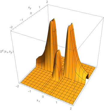
Figure 1 1 1 y 𝑦 y 𝐒 𝐲 ( k → , k z ; δ t ) superscript 𝐒 𝐲 → 𝑘 subscript 𝑘 𝑧 𝛿 𝑡 \mathbf{S^{y}}(\vec{k},k_{z};\delta t) k 1 = k x subscript 𝑘 1 subscript 𝑘 𝑥 k_{1}=k_{x} k 2 = k y subscript 𝑘 2 subscript 𝑘 𝑦 k_{2}=k_{y} μ = 0.5 e v . 𝜇 0.5 𝑒 𝑣 \mu=0.5ev. M = ± 0.3 e V 𝑀 plus-or-minus 0.3 𝑒 𝑉 M=\pm 0.3eV
Figure 1: The y polarization of the emitted electons given by 𝐒 𝐲 ( k → , k z ) superscript 𝐒 𝐲 → 𝑘 subscript 𝑘 𝑧 \mathbf{S^{y}}(\vec{k},k_{z}) k x subscript 𝑘 𝑥 k_{x} k y subscript 𝑘 𝑦 k_{y} μ = 0.5 𝜇 0.5 \mu=0.5 W 𝑊 W ℏ Ω Planck-constant-over-2-pi Ω \hbar\Omega
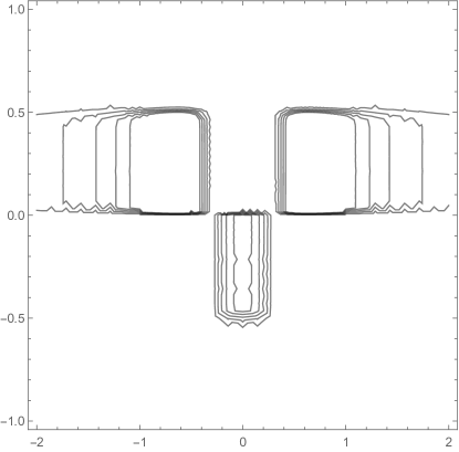
The plot in figure ( 3 ) 3 (3) ( 1 ) 1 (1) S y − μ superscript 𝑆 𝑦 𝜇 S^{y}-\mu k 2 subscript 𝑘 2 k_{2} k 1 subscript 𝑘 1 k_{1} ( 2 ) 2 (2) k 1 = ± 0.3 subscript 𝑘 1 plus-or-minus 0.3 k_{1}=\pm 0.3 k 1 = 0.3 subscript 𝑘 1 0.3 k_{1}=0.3 k 1 = − 0.3 subscript 𝑘 1 0.3 k_{1}=-0.3 0 = k 2 → k 2 = − 0.5 → k 2 = 0 0 subscript 𝑘 2 → subscript 𝑘 2 0.5 → subscript 𝑘 2 0 0=k_{2}\rightarrow k_{2}=-0.5\rightarrow k_{2}=0 1 1 1 μ = 0.5 𝜇 0.5 \mu=0.5 ( 2 ) 2 (2) μ = 0 𝜇 0 \mu=0 k 2 = 0 subscript 𝑘 2 0 k_{2}=0 μ > 0 𝜇 0 \mu>0 k 1 = M subscript 𝑘 1 𝑀 k_{1}=M k 1 = − M subscript 𝑘 1 𝑀 k_{1}=-M 0 = k 2 → k 2 = − μ → k 2 = 0 0 subscript 𝑘 2 → subscript 𝑘 2 𝜇 → subscript 𝑘 2 0 0=k_{2}\rightarrow k_{2}=-\mu\rightarrow k_{2}=0
Figure 2: -The Fermi arc- a two dimensional contour 𝐒 𝐲 ( k → ) superscript 𝐒 𝐲 → 𝑘 \mathbf{S^{y}}(\vec{k})
The suggested three dimensional chiral anomaly and the detection in photoemission Grushin z = 0 𝑧 0 z=0 n R ( k 2 ) subscript 𝑛 𝑅 subscript 𝑘 2 n_{R}(k_{2}) n L ( k 2 ) subscript 𝑛 𝐿 subscript 𝑘 2 n_{L}(k_{2}) N R subscript 𝑁 𝑅 N_{R} N L subscript 𝑁 𝐿 N_{L} n R ( k 2 ) = 1 e β ℏ v ( k 2 ) ( k 2 − k F ) + 1 subscript 𝑛 𝑅 subscript 𝑘 2 1 superscript 𝑒 𝛽 Planck-constant-over-2-pi 𝑣 subscript 𝑘 2 subscript 𝑘 2 subscript 𝑘 𝐹 1 n_{R}(k_{2})=\frac{1}{e^{\beta\hbar v(k_{2})(k_{2}-k_{F})}+1} N R = L ∫ 0 ∞ d ϵ h v ( k 2 ) n R ( k 2 ) subscript 𝑁 𝑅 𝐿 superscript subscript 0 𝑑 italic-ϵ ℎ 𝑣 subscript 𝑘 2 subscript 𝑛 𝑅 subscript 𝑘 2 N_{R}=L\int_{0}^{\infty}\frac{d\epsilon}{hv(k_{2})}n_{R}(k_{2}) ϵ = ℏ v ( k 2 ) ( k 2 ) italic-ϵ Planck-constant-over-2-pi 𝑣 subscript 𝑘 2 subscript 𝑘 2 \epsilon=\hbar v(k_{2})(k_{2}) d N R d t = L ∫ 0 ∞ d ϵ h v ( k 2 ) d n R ( k 2 ) d ϵ d ϵ d t 𝑑 subscript 𝑁 𝑅 𝑑 𝑡 𝐿 superscript subscript 0 𝑑 italic-ϵ ℎ 𝑣 subscript 𝑘 2 𝑑 subscript 𝑛 𝑅 subscript 𝑘 2 𝑑 italic-ϵ 𝑑 italic-ϵ 𝑑 𝑡 \frac{dN_{R}}{dt}=L\int_{0}^{\infty}\frac{d\epsilon}{hv(k_{2})}\frac{dn_{R}(k_{2})}{d\epsilon}\frac{d\epsilon}{dt} d k 2 d t = − e ℏ E 2 𝑑 subscript 𝑘 2 𝑑 𝑡 𝑒 Planck-constant-over-2-pi subscript 𝐸 2 \frac{dk_{2}}{dt}=\frac{-e}{\hbar}E_{2} 1 L d ( N R − N L ) d t = ( 1 e − β ϵ F + 1 ) ( − e ℏ E 2 ) T → 0 = − e ℏ E 2 1 𝐿 𝑑 subscript 𝑁 𝑅 subscript 𝑁 𝐿 𝑑 𝑡 1 superscript 𝑒 𝛽 subscript italic-ϵ 𝐹 1 subscript 𝑒 Planck-constant-over-2-pi subscript 𝐸 2 → 𝑇 0 𝑒 Planck-constant-over-2-pi subscript 𝐸 2 \frac{1}{L}\frac{d(N_{R}-N_{L})}{dt}=(\frac{1}{e^{-\beta\epsilon_{F}}+1})\Big{(}\frac{-e}{\hbar}E_{2}\Big{)}_{T\rightarrow 0}=\frac{-e}{\hbar}E_{2}
We assume i n t e r − v a l l e y 𝑖 𝑛 𝑡 𝑒 𝑟 𝑣 𝑎 𝑙 𝑙 𝑒 𝑦 inter-valley τ v subscript 𝜏 𝑣 \tau_{v} d N R d t c o l l i s i o n = − 1 τ v ( N R − N R 0 ) subscript 𝑑 subscript 𝑁 𝑅 𝑑 𝑡 𝑐 𝑜 𝑙 𝑙 𝑖 𝑠 𝑖 𝑜 𝑛 1 subscript 𝜏 𝑣 subscript 𝑁 𝑅 subscript superscript 𝑁 0 𝑅 \frac{dN_{R}}{dt}_{collision}=-\frac{1}{\tau_{v}}\Big{(}N_{R}-N^{0}_{R}\Big{)} N R = N R 0 ( ϵ F + δ μ R ) subscript 𝑁 𝑅 subscript superscript 𝑁 0 𝑅 subscript italic-ϵ 𝐹 𝛿 subscript 𝜇 𝑅 N_{R}=N^{0}_{R}(\epsilon_{F}+\delta\mu_{R}) − e ℏ E 2 = d ( N R − N L ) d t = − 1 τ v ( N R 0 ( ϵ F + δ μ R ) − N L 0 ( ϵ F + δ μ L ) ) 𝑒 Planck-constant-over-2-pi subscript 𝐸 2 𝑑 subscript 𝑁 𝑅 subscript 𝑁 𝐿 𝑑 𝑡 1 subscript 𝜏 𝑣 subscript superscript 𝑁 0 𝑅 subscript italic-ϵ 𝐹 𝛿 subscript 𝜇 𝑅 subscript superscript 𝑁 0 𝐿 subscript italic-ϵ 𝐹 𝛿 subscript 𝜇 𝐿 \frac{-e}{\hbar}E_{2}=\frac{d(N_{R}-N_{L})}{dt}=-\frac{1}{\tau_{v}}\Big{(}N^{0}_{R}(\epsilon_{F}+\delta\mu_{R})-N^{0}_{L}(\epsilon_{F}+\delta\mu_{L})\Big{)} δ μ R − δ μ L = e v F τ v E 2 𝛿 subscript 𝜇 𝑅 𝛿 subscript 𝜇 𝐿 𝑒 subscript 𝑣 𝐹 subscript 𝜏 𝑣 subscript 𝐸 2 \delta\mu_{R}-\delta\mu_{L}=ev_{F}\tau_{v}E_{2}
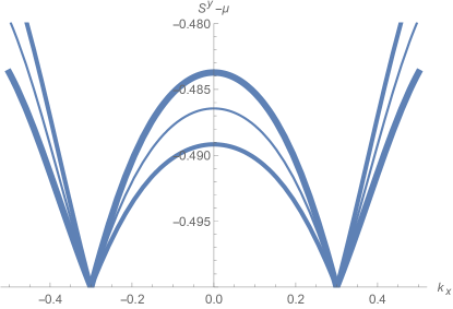
We have checked the effect of the chiral anomaly on the photoemission spectrum by using the shift of the chemical potential δ = δ μ L = − δ μ R = v F τ v 2 ( − e ℏ ) E 2 𝛿 𝛿 subscript 𝜇 𝐿 𝛿 subscript 𝜇 𝑅 subscript 𝑣 𝐹 subscript 𝜏 𝑣 2 𝑒 Planck-constant-over-2-pi subscript 𝐸 2 \delta=\delta\mu_{L}=-\delta\mu_{R}=\frac{v_{F}\tau_{v}}{2}(\frac{-e}{\hbar})E_{2} δ 𝛿 \delta S y − μ superscript 𝑆 𝑦 𝜇 S^{y}-\mu δ = 0 𝛿 0 \delta=0 ( 2 ) 2 (2) ( 2 ) 2 (2) δ = ± 0.05 e v 𝛿 plus-or-minus 0.05 𝑒 𝑣 \delta=\pm 0.05ev
Figure 3: The plot of 𝐒 𝐲 ( k x ) superscript 𝐒 𝐲 subscript 𝑘 𝑥 \mathbf{S^{y}}(k_{x}) δ = 0.05 𝛿 0.05 \delta=0.05 δ = 0.0 𝛿 0.0 \delta=0.0 δ = − 0.05 𝛿 0.05 \delta=-0.05
To conclude we have demonstrate theoretically the emergence of the fermi arcs and their manipulation with the help of the one dimensional chiral anomaly. This has been achieved with the helped of an Hamiltonian which consider the connection between the two nodes and a wave function which respect the boundary conditions in the presence of a surface at z = 0 𝑧 0 z=0
References
(1)
H. Weyl Z.Phys.56 330 (1929).
(2)
X. Wan, A.M. Turner, A. Vishwanath, and S.Y.Savrasov Phys.Rev.B. 83 , 205101 (2011).
(3)
G.Xu,H.Weng,Z.Wang,X.Dai and Z.Fang ,Phys.Rev.Lett. 107 , 186806 (2011).
(4)
H.Nielsen and M.Ninomiya,Phys.Lett. B 130 , 389 (1983).
(5)
Su-Yang Xu, Ilya Belopolski,Nasser Alidoust, Madhab Neupaine, Guang Bian, Chenlong ,Raman Sankar, Guoqing Chang, Zhujun Yuan, Chi-Cheng Lee, Shin-Ming Huang,Hao Zheng, Jie Ma, Daniel S.Sanchez, BaoKai Wang, Arun Bansil, Fangcheng Chou, Pavel P.Shibayev, Hsin Lin, Shuang Jia, M.Zahid Hasan
Science, vol. 349 ISSUE 6248 (2015)
(6)
Rajib Batabyal,Noam Morali, Nurit Avraham, Yan Sun, Marcus Schmidt, Caudia Felser, Ady Stern, Binghai Yan, Haim Beidenkopf Sci. Adv. 2, e1600709 (2016).
(7)
Dan Thahn Son and Naoki Yamato Phys.Rev.Lett. 109 , 181602 (2012).
(8)
D.T.Son and B.Spivak Phys.Rev.B 88 ,104412 (2013)
(9)
T.C. Chiang ,J.A.Knapp, M.Aono and D.E. Eastman Phys.Rev.B 21 , 3513 (1979).
(10)
D.Schmeltzer and A.Saxena Journal of Physics ,Condensed Matter 27 485601 (2015).
(11)
Jan Behrends,Adolpho G.Grushin , Teemu Ojanen and Jens H. Badarson Phys. Rev.B 93 ,075114
(2015)