Death and rebirth of neural activity in sparse inhibitory networks

Abstract

Inhibition is a key aspect of neural dynamics playing a fundamental role for the emergence of neural rhythms and the implementation of various information coding strategies. Inhibitory populations are present in several brain structures and the comprehension of their dynamics is strategical for the understanding of neural processing. In this paper, we clarify the mechanisms underlying a general phenomenon present in pulse-coupled heterogeneous inhibitory networks: inhibition can induce not only suppression of the neural activity, as expected, but it can also promote neural reactivation. In particular, for globally coupled systems, the number of firing neurons monotonically reduces upon increasing the strength of inhibition (neurons’ death). However, the random pruning of the connections is able to reverse the action of inhibition, i.e. in a random sparse network a sufficiently strong synaptic strength can surprisingly promote, rather than depress, the activity of the neurons (neurons’ rebirth). Thus the number of firing neurons reveals a minimum at some intermediate synaptic strength. We show that this minimum signals a transition from a regime dominated by the neurons with higher firing activity to a phase where all neurons are effectively sub-threshold and their irregular firing is driven by current fluctuations. We explain the origin of the transition by deriving a mean field formulation of the problem able to provide the fraction of active neurons as well as the first two moments of their firing statistics. The introduction of a synaptic time scale does not modify the main aspects of the reported phenomenon. However, for sufficiently slow synapses the transition becomes dramatic, the system passes from a perfectly regular evolution to an irregular bursting dynamics. In this latter regime the model provides predictions consistent with experimental findings for a specific class of neurons, namely the medium spiny neurons in the striatum.

I Introduction

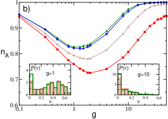
Figure 1: a-b) Fraction of active neurons $n_{A}$ as a function of the inhibitory synaptic strength $g$ for a globally coupled system (a), where $K=N-1$, and a randomly connected (sparse) network with $K=20$ (b). In a) is reported the asymptotic value $n_{A}$ calculated after a time $t_{S}=1\times 10^{6}$. Conversely in b), $n_{A}$ is reported at successive times: namely, $t_{S}=985$ (red squares), $t_{S}=1.1\times 10^{4}$ (brown stars), $t_{S}=5\times 10^{5}$ (blue diamonds) and $t_{S}=1\times 10^{6}$ (green triangles). An estimation of the times needed to reach $n_{A}=1$ can be obtained by employing Eq. (13) these values range from $t_{s}=5\times 10^{9}$ for $g=0.1$ to $5\times 10^{5}$ for $g=50$. Insets in b) depict the probability distributions $P(\nu)$ of the single neuron firing rate $\nu$ for the sparse network for a given $g$ indicated in the inset at two different times: $t_{S}=985$ (red filled histograms) and $t_{S}=1\times 10^{6}$ (thick empty green histograms). The histograms are calculated by considering only active neurons. The reported data refer to instantaneous synapses, to a system size $N=400$ and to an uniform distribution $P(I)$ with $[l_{1},l_{2}]=[1.0,1.5]$ and $\theta=1$, the values reported in a) and b) have been also averaged over 10 random realizations of the network.

The presence of inhibition in excitable systems induces a rich dynamical repertoire, which is extremely relevant for biological camazine2003 , physical kerner1990 and chemical systems vanag2000 . In particular, inhibitory coupling has been invoked to explain cell navigation xiong2010cells , morphogenesis in animal coat pattern formation meinhardt1982 , and the rhythmic activity of central pattern generators in many biological systems harris1992 ; marder2001 . In brain circuits the role of inhibition is fundamental to balance massive recurrent excitation somogyi1998salient in order to generate physiologically relevant cortical rhythms shu2003turning ; buz2004 .

Inhibitory networks are important not only for the emergence of rhythms in the brain, but also for the fundamental role they play in information encoding in the olfactory system laurent2002olfactory as well as in controlling and regulating motor and learning activity in the basal ganglia berke2004oscillatory ; miller2008dysregulated ; carrillo2008encoding . Furthermore, stimulus dependent sequential activation of neurons or group of neurons, reported for asymmetrically connected inhibitory cells nowotny2007dynamical ; komarov2009sequentially , has been suggested as a possible mechanism to explain sequential memory storage and feature binding  rabinovich2011 .

These explain the long term interest for numerical and theoretical investigations of the dynamics of inhibitory networks. Already the study of globally coupled homogeneous systems revealed interesting dynamical features, ranging from full synchronization to clustering appearance golomb1994clustering ; vanVreeswijk1996Partial ; wang1996gamma , from the emergence of splay states Zillmer2006 to oscillator death bressloff2000dynamics . The introduction of disorder, e.g. random dilution, noise or other form of heterogeneity in these systems leads to more complex dynamics, ranging from fast global oscillations BrunelHakim1999 in neural networks and self-sustained activity in excitable systems larremore2014 , to irregular dynamics Zillmer2006 ; JhankeTimme2008PRL ; Timme2009ChaosBalance ; MonteforteBalanced2012 ; Luccioli2010Irregular ; angulo2014 ; ostojic2014 ; kadmon2015 ; ullner2016self . In particular, inhibitory spiking networks, due to stable chaos politi2010stable , can display extremely long erratic transients even in linearly stable regimes Zillmer2006 ; Zillmer2009LongTrans ; JhankeTimme2008PRL ; Timme2009ChaosBalance ; MonteforteBalanced2012 ; angulo2014 ; ullner2016self ; Luccioli2010Irregular .

One of the most studied inhibitory neural population is represented by medium spiny neurons (MSNs) in the striatum (which is the main input structure of the basal ganglia) parent1995functional ; lanciego2012functional . In a series of papers, Ponzi and Wickens have shown that the main features of the MSN dynamics can be reproduced by considering a randomly connected inhibitory network of conductance based neurons subject to external stochastic excitatory inputs ponzi2010sequentially ; ponzi2012input ; ponzi2013optimal . Our study has been motivated by an interesting phenomenon reported for this model in ponzi2013optimal : namely, upon increasing the synaptic strength the system passes from a regularly firing regime, characterized by a large part of quiescent neurons, to a biologically relevant regime where almost all cells exhibit a bursting activity, characterized by an alternation of periods of silence and of high firing. The same phenomenology has been recently reproduced by employing a much simpler neural model angulo2015Striatum . Thus suggesting that this behaviour is not related to the specific model employed, but it is indeed a quite general property of inhibitory networks. However, it is still unclear the origin of the phenomenon and the minimal ingredients required to observe the emergence of this effect.

In order to exemplify the problem addressed in this paper we report in Fig. 1 the fraction of active neurons $n_{A}$ (i.e. the ones emitting at least one spike during the simulation time) as a function of the strength of the synaptic inhibition $g$ in an heterogeneous network. For a fully coupled network, $n_{A}$ has a monotonic decrease with $g$ (Fig. 1 (a)), while for a random sparse network $n_{A}$ has a non monotonic behaviour, displaying a minimum at an intermediate strength $g_{m}$ (Fig. 1 (b)). In fully coupled networks the effect of inhibition is simply to reduce the number of active neurons (neurons’ death). However, quite counter-intuitively, in presence of dilution by increasing the synaptic strength the previously silenced neurons can return to fire (neurons’ rebirth). Our aim is to clarify the physical mechanisms underlying neuron’s death and rebirth, which are at the origin of the behaviour reported in  ponzi2013optimal ; angulo2015Striatum .

In particular, we consider a deterministic network of purely inhibitory pulse-coupled Leaky Integrate-and-Fire (LIF) neurons with an heterogeneous distribution of excitatory DC currents, accounting for the different level of excitability of the neurons. The evolution of this model is studied for fully coupled and for random sparse topology, as well as for synapses with different time courses. For the fully coupled case, it is possible to derive, within a self-consistent mean field approach, the analytic expressions for the fraction of active neurons and for the average firing frequency ${\bar{\nu}}$ as a function of the coupling strength $g$. In this case the monotonic decrease of $n_{A}$ with $g$ can be interpreted as a Winner Takes All (WTA) mechanism fukai1997simple ; coultrip1992cortical ; yuille1989 , where only the most excitable neurons survive to the inhibition increase. For random sparse networks, the neurons’ rebirth can be interpreted as a re-activation process induced by erratic fluctuations in the synaptic currents. Within this framework it is possible to obtain semi-analytically, for instantaneous synapses, a closed set of equations for $n_{A}$ as well as for the average firing rate and coefficient of variation as a function of the coupling strength. In particular, the firing statistics of the network can be obtained via a mean-field approach by extending the formulation derived in richardson2010firing to account for synaptic shot noise with constant amplitude. The introduction of a finite synaptic time scale do not modify the overall scenario as far as this is shorter than the membrane time constant. As soon as the synaptic dynamics becomes slower, the phenomenology of the transition is modified. At $g<g_{m}$ we have a frozen phase where $n_{A}$ does not evolve in time on the explored time scales, since the current fluctuations are negligible. Above $g_{m}$ we have a bursting regime, which can be related to the emergence of correlated fluctuations induced by slow synaptic times, as discussed in the framework of the adiabatic approach in moreno2004 ; moreno2010response .

The paper is organized as follows: In Sect. II we present the models that will be considered in the paper as well as the methods adopted to characterize its dynamics. In Sect. III we consider the globally coupled network where we provide analytic self-consistent expressions accounting for the fraction of active neurons and the average firing rate. Section IV is devoted to the study of sparsely connected networks with instantaneous synapses and to the derivation of the set of semi-analytic self-consistent equations providing $n_{A}$, the average firing rate and the coefficient of variation. In section V we discuss the effect of synaptic filtering with a particular attention on slow synapses. Finally in Sect. VI we briefly discuss the obtained results with a focus on the biological relevance of our model.

II Model and Methods

We examine the dynamical properties of an heterogeneous inhibitory sparse network made of $N$ LIF neurons. The time evolution of the membrane potential $v_{i}$ of the $i$-th neuron is ruled by the following first order ordinary differential equation:

$$\dot{v}_{i}(t)=I_{i}-v_{i}(t)-gE_{i}(t)\qquad;$$ (1)

where $g>0$ is the inhibitory synaptic strength, $I_{i}$ is the neuronal excitability of the $i$-th neuron encompassing both the intrinsic neuronal properties and the excitatory stimuli originating from areas outside the considered neural circuit and $E_{i}(t)$ represents the synaptic current due to the recurrent interactions within the considered network. The membrane potential $v_{i}$ of neuron $i$ evolves accordingly to Eq. (1) until it overcomes a constant threshold $\theta=1$, this leads to the emission of a spike (action potential) transmitted to all the connected post-synaptic neurons, while $v_{i}$ is reset to its rest value $v_{r}=0$. The model in (1) is expressed in adimensional units, this amounts to assume a membrane time constant $\tau_{m}=1$, for the conversion to dimensional variables see Appendix A. The heterogeneity is introduced in the model by assigning to each neuron a different value of input excitability $I_{i}$ drawn from a flat distribution $P(I)$, whose support is $I\in[l_{1},l_{2}]$ with $l_{1}\geq\theta$, therefore all the neurons are supra-threshold.

The synaptic current $E_{i}(t)$ is given by the linear super-position of all the inhibitory post-synaptic potentials (IPSPs) $\eta(t)$ emitted at previous times $t_{n}^{j}<t$ by the pre-synaptic neurons connected to neuron $i$, namely

$$E_{i}(t)=\frac{1}{K}\sum_{j\neq i}C_{ij}\sum_{n|t_{n}<t}\eta(t-t^{j}_{n})\;;$$ (2)

where $K$ is the number of pre-synaptic neurons. $C_{ij}$ represent the elements of the $N\times N$ connectivity matrix associated to an undirected random network, whose entries are $1$ if there is a synaptic connection from neuron $j$ to neuron $i$, and $0$ otherwise. For the sparse network, we select randomly the matrix entries, however to reduce the sources of variability in the network, we assume that the number of pre-synaptic neurons is fixed, namely $\sum_{j\neq i}C_{ij}=K<<N$ for each neuron $i$, where autaptic connections are not allowed. We have verified that the results do not change if we choose randomly the links accordingly to an Erdös-Renyi distribution with a probability $K/N$. For a fully coupled network we have $K=N-1$.

The shape of the IPSP characterize the type of filtering performed by the synapses on the received action potentials. We have considered two kind of synapses, instantaneous ones, where $\eta(t)=\delta(t)$, and synapses where the PSP is an $\alpha$-pulse, namely

$$\eta(t)=H(t){\alpha}^{2}t{\rm e}^{-t{\alpha}}\qquad;$$ (3)

with $H$ denoting the Heaviside step function. In this latter case the rise and decay time of the pulse are the same, namely $\tau_{\alpha}=1/\alpha$, and therefore the pulse duration $\tau_{P}$ can be assumed to be twice the characteristic time $\tau_{\alpha}$. The equations of the model Eqs. (1) and (2) are integrated exactly in terms of the associated event driven maps for different synaptic filtering, these correspond to Poincaré maps performed at the firing times (for details see Appendix A) Zillmer2007 ; Olmi2014linear .

For instantaneous synapses, we have usually considered system sizes $N=400$ and $N=1,400$ and for the sparse case in-degrees $20\leq K\leq 80$ for $N=400$ and $20\leq K\leq 600$ for $N=1400$ with integration times up to $t_{S}=1\times 10^{6}$. For synapses with a finite decay time we limit the analysis to $N=400$ and $K=20$ and to maximal integration times $t_{S}=1\times 10^{5}$. Finite size dependences on $N$ are negligible with these parameter choices, as we have verified.

In order to characterize the network dynamics we measure the fraction of active neurons $n_{A}(t_{S})$ at time $t_{S}$, i.e. the fraction of neurons emitting at least one spike in the time interval $[0,t_{S}]$. Therefore a neuron will be considered silent if it has a frequency smaller than $1/t_{S}$, with our choices of $t_{S}=10^{5}-10^{6}$, this corresponds to neurons with frequencies smaller than $10^{-3}-10^{-4}$ Hz, by assuming as timescale a membrane time constant $\tau_{m}=10$ ms. The estimation of the number of active neurons is always started after a sufficiently long transient time has been discarded, usually corresponding to the time needed to deliver $10^{6}$ spikes in the network.

Furthermore, for each neuron we estimate the time averaged inter-spike interval (ISI) $T_{ISI}$, the associated firing frequency $\nu=1/T_{ISI}$, as well as the coefficient of variation $CV$, which is the ratio of the standard deviation of the ISI distribution divided by $T_{ISI}$. For a regular spike train $CV=0$, for a Poissonian distributed one $CV=1$, while $CV>1$ is an indication of bursting activity. The indicators usually reported in the following to characterize the network activity are ensemble averages over all the active neurons, which we denote as $\bar{a}$ for a generic observable $a$.

To analyze the linear stability of the dynamical evolution we measure the maximal Lyapunov exponent $\lambda$, which is positive for chaotic evolution, and negative (zero) for stable (marginally stable) dynamics (BenettinLyapunov1980, ). In particular, by following Olmi2010Oscillations ; angulo2015stochastic $\lambda$ is estimated by linearizing the corresponding event driven map.

III Fully Coupled Networks:
Winner Takes All

In the fully coupled case we observe that the number of active neurons $n_{A}$ saturates, after a short transient, to a value which remains constant in time. In this case, it is possible to derive a self-consistent mean field approach to obtain analytic expressions for the fraction of active neurons $n_{A}$ and for the average firing frequency $\bar{\nu}$ of the neurons in the network. In a fully coupled network each neuron receives the spikes emitted by the other $K=N-1$ neurons, therefore each neuron is essentially subject to the same effective input $\mu$, apart corrections ${\cal O}(1/N)$.

The effective input current, for a neuron with an excitability $I$, is given by

$$\mu=I-g\bar{\nu}n_{A}\;\quad;$$ (4)

where $n_{A}(N-1)$ is the number of active pre-synaptic neurons assumed to fire with the same average frequency $\bar{\nu}$.

In a mean field approach, each neuron can be seen as isolated from the network and driven by the effective input current $\mu$. Taking into account the distribution of the excitabilities $P(I)$ one obtains the following self-consistent expression for the average firing frequency

$$\bar{\nu}=\frac{1}{\Delta}\int_{\{I_{A}\}}dI\enskip P(I)\left[\ln\left(\frac{I-g\bar{\nu}n_{A}-v_{r}}{I-g\bar{\nu}n_{A}-\theta}\right)\right]^{-1}$$ (5)

where the integral is restricted only to active neurons, i.e. to $I\in\{I_{A}\}$ values for which the logarithm is defined, while $\Delta=\int_{\{I_{A}\}}dI\enskip P(I)$ is the measure of their support. In (5) we have used the fact that for an isolated LIF neuron with constant excitability $C$, the ISI is simply given by $T_{ISI}=\ln[(C-v_{r})/(C-\theta)]$ burkitt2006LIFreviewI .

An implicit expression for $n_{A}$ can be obtained by estimating the neurons with effective input $\mu>\theta$, in particular the number of silent neurons is given by

$$1-n_{A}=\int_{l_{1}}^{l^{*}}dIP(I)\;,$$ (6)

where $l_{1}$ is the lower limit of the support of the distribution, while $l^{*}=g\bar{\nu}n_{A}+\theta$. By solving self-consistently Eqs.(5) and (6) one can obtain the analytic expression for $n_{A}$ and $\bar{\nu}$ for any distribution $P(I)$.

In particular, for excitabilities distributed uniformly in the interval $[l_{1},l_{2}]$, the expression for the average frequency Eq. (5) becomes

$$\bar{\nu} = \frac{1}{n_{A}(l_{2}-l_{1})}\int_{\{I_{A}\}}dI\left[\ln\left(\frac{I-g\bar{\nu}n_{A}-v_{r}}{I-g\bar{\nu}n_{A}-\theta}\right)\right]^{-1}\quad;$$ (7)

while the number of active neurons is given by the following expression

$$n_{A}=\frac{l_{2}-\theta}{l_{2}-l_{1}+g\bar{\nu}}\quad;$$ (8)

with the constraint that $n_{A}$ cannot be larger than one.

The analytic results for these quantities compare quite well with the numerical findings estimated for different distribution intervals $[l_{1},l_{2}]$, different coupling strengths and system sizes, as shown in Fig. 2. Apart for definitely large coupling $g>10$ where some discrepancies among the mean field estimations and the simulation results for $\bar{\nu}$ are observable (see Fig. 2 (b)). These differences are probably due to the discreteness of the pulses, which cannot be neglected for very large synaptic strengths.

As a general feature we observe that $n_{A}$ is steadily decreasing with $g$, thus indicating that a group of neurons with higher effective inputs (winners) silence the other neurons (losers) and that the number of winners eventually vanishes for sufficiently large coupling in the limit of large system sizes. Furthermore, the average excitability of the active neurons (the winners) $\bar{I}_{A}$ increases with $g$, as shown in the inset of Fig. 2 (a), thus revealing that only the neurons with higher excitabilities survive to the silencing action exerted by the other neurons. At the same time, as an effect of the growing inhibition the average firing rate of the winners dramatically slows down. Therefore despite the increase of $\bar{I}_{A}$ the average effective input $\bar{\mu}$ indeed decreases for increasing inhibition. This represents a clear example of the winner takes all (WTA) mechanism obtained via (lateral) inhibition, which has been shown to have biological relevance for neural systems yuille1989 ; ermentrout1992 ; fukai1997 ; plenz2003 .

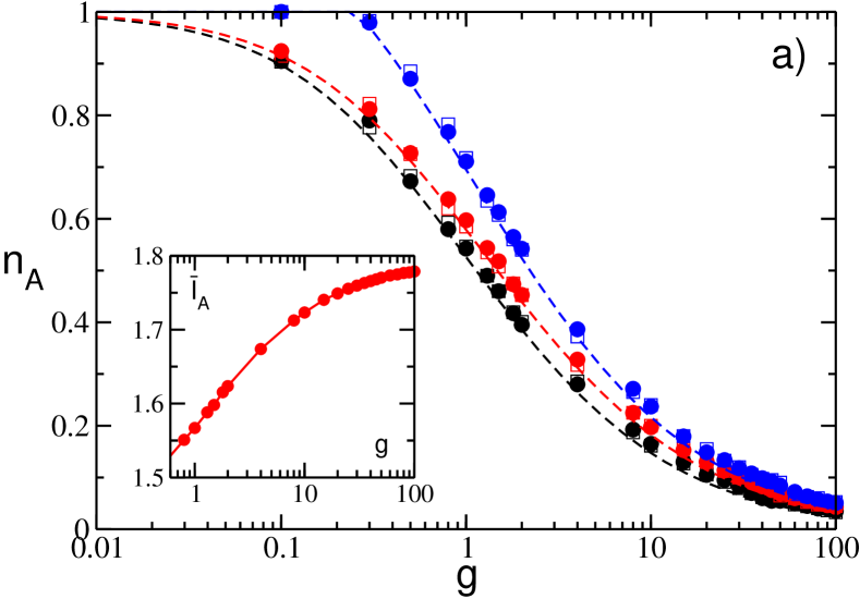
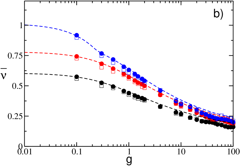
Figure 2: Fraction of active neurons $n_{A}$ (a) and average network’s frequency $\bar{\nu}$ (b) as a function of the synaptic strength $g$ for uniform distributions $P(I)$ with different supports. Inset: average neuronal excitability of the active neurons $\bar{I}_{A}$ versus $g$. Empty (filled) symbols refer to numerical simulation with $N=400$ ($N=1400$) and dashed lines to the corresponding analytic solution. Symbols and lines correspond from bottom to top to $[l_{1},l_{2}]=[1.0,1.5]$ (black); $[l_{1},l_{2}]=[1.0,1.8]$ (red) and $[l_{1},l_{2}]=[1.2,2.0]$ (blue). The data have been averaged over a time interval $t_{S}=1\times 10^{6}$ after discarding a transient of $10^{6}$ spikes.

It is important to understand which is the minimal coupling value $g_{c}$ for which the firing neurons start to die. In order to estimate $g_{c}$ it is sufficient to set $n_{A}=1$ in Eqs. (7) and (8). In particular, one gets

$$g_{c}=(l_{1}-\theta)/\bar{\nu}\quad,$$ (9)

thus for $l_{1}=\theta$ even an infinitesimally small coupling is in principle sufficient to silence some neurons. Furthermore, from Fig. 3 (a) it is evident that whenever the excitabilities become homogeneous, i.e. for $l_{1}\to l_{2}$, the critical synaptic coupling $g_{c}$ diverges towards infinity. Thus heterogeneity in the excitability distribution is a necessary condition in order to observe a gradual neurons’ death, as shown in Fig. 2 (a).

This is in agreement with the results reported in  bressloff2000 , where homogeneous fully coupled networks of inhibitory LIF neurons have been examined. In particular, for finite systems and slow synapses the authors in bressloff2000 reveal the existence of a sub-critical Hopf bifurcation from a fully synchronized state to a regime characterized by oscillator death occurring at some critical $g_{c}$. However, in the thermodynamic limit $g_{c}\to\infty$ for fast as well as slow synapses, in agreement with our mean field result for instantaneous synapses.

We also proceed to investigate the isolines corresponding to the same critical $g_{c}$ in the $(l_{1},l_{2})$-plane, the results are reported in Fig. 3 (b) for three selected values of $g_{c}$. It is evident that the $l_{1}$ and $l_{2}$-values associated to the isolines display a direct proportionality among them. However, despite lying on the same $g_{c}$-isoline, different parameter values induce a completely different behaviour of $n_{A}$ as a function of the synaptic strength, as shown in the inset of Fig. 3 (b).

Direct simulations of the network at finite sizes, namely for $N=400$ and $N=1400$, show that for sufficiently large coupling neurons with similar excitabilities tend to form clusters, similarly to what reported in Luccioli2010Irregular , for the same model here studied, but with a delayed pulse transmission. However, at variance with Luccioli2010Irregular , the overall macroscopic dynamics is asynchronous and no collective oscillations can be detected for the whole range of considered synaptic strengths.

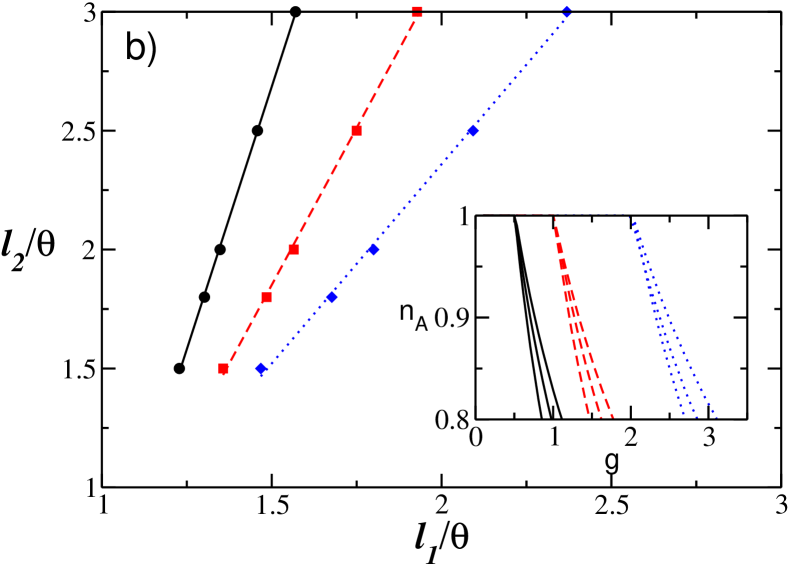
Figure 3: a) Critical value $g_{c}$ as a function of the lower value of the excitability $l_{1}$ for several choices of the upper limit $l_{2}$. b) Isolines corresponding to constant values of $g_{c}$ in the $(l_{1},l_{2})$-plane: namely, $g_{c}=0.5$ (black solid line), $g_{c}=1.0$ (red dashed line), $g_{c}=2.0$ (blue dotted line). Inset: Dependence of $n_{A}$ on $g$ for three couples of values $(l_{1},l_{2})$ chosen along each of the isolines reported in the main figure.

IV Sparse Networks :
Neurons’ rebirth

In this Section we will consider a network with sparse connectivity, namely each neuron is supra-threshold and it receives instantaneous IPSPs from $K<<N$ randomly chosen neurons in the network. Due to the sparseness, the input spike trains can be considered as uncorrelated and at a first approximation it can be assumed that each spike train is Poissonian with a frequency $\bar{\nu}$ correspondent to the average firing rate of the neurons in the network BrunelHakim1999 ; Brunel2000Sparse . Usually, the mean activity of a LIF neural network has been estimated in the context of the diffusion approximation ricciardi2013diffusion ; tuckwell2005 . This approximation is valid whenever the arrival frequency of the IPSPs is high with respect to the firing emission, while the amplitude of each IPSPs (namely, $G=g/K$) is small with respect to the firing threshold $\theta$. This latter hypothesis in our case is not valid for sufficiently large (small) synaptic strength $g$ (in-degree $K$), as it can be appreciated by the comparison shown in Fig. 13 in Appendix B. Therefore the synaptic inputs should be treated as shot noise. In particular, here we apply an extended version of the analytic approach derived by Richardson and Swabrick in richardson2010firing to estimate the average firing rate and the average coefficient of variation for LIF neurons with instantaneous synapses subject to inhibitory shot noise of constant amplitude (for more details see Appendices B and C).

At variance with the fully coupled case, the fraction of active neurons $n_{A}$ does not saturate to a constant value for sufficiently short times. Instead, $n_{A}$ increases in time, due to the rebirth of losers which have been previously silenced by the firing activity of the winners, as shown in in Fig. 1(b). This effect is clearly illustrated by considering the probability distributions $P(\nu)$ of the firing rates of the neurons at successive integration times $t_{S}$. These are reported in the insets of Fig 1(b) for two coupling strengths and two times: namely, $t_{S}=985$ (red lines) and $t_{S}=1\times 10^{6}$ (green lines). From these data is evident that the fraction of neurons with low firing rate (the losers) increases in time, while the fraction of high firing neurons remains almost unchanged. Moreover, the variation of $n_{A}$ slows down for increasing $t_{S}$ and $n_{A}$ approaches some apparently asymptotic profile for sufficiently long integration times. Furthermore, $n_{A}$ has a non monotonic behaviour with $g$, as opposite to the fully coupled case. In particular, $n_{A}$ reveals a minimum $n_{A_{m}}$ at some intermediate synaptic strength $g_{m}$ followed by an increase towards $n_{A}=1$ at large $g$. As we have verified, as far as $1<K<<N$ finite size effects are negligible and the actual value of $n_{A}$ depends only on the in-degree $K$ and the considered simulation time $t_{S}$. In the following we will try to explain the origin of such a behaviour.

Despite the model is fully deterministic, due to the random connectivity the rebirth of silent neurons can be interpreted in the framework of activation processes induced by random fluctuations. In particular, we can assume that each neuron in the network will receive $n_{A}K$ independent Poissonian trains of inhibitory kicks of constant amplitude $G$ characterized by an average frequency $\bar{\nu}$ , thus each synaptic input can be regarded as a single Poissonian train with total frequency $R=n_{A}K\bar{\nu}$. Therefore, each neuron, characterized by its own excitability $I$, will be subject to an average effective input $\mu(I)$ (as reported in Eq.  (4)) plus fluctuations in the synaptic current of intensity

$$\sigma=g\sqrt{\frac{n_{A}\bar{\nu}}{K}}\qquad.$$ (10)

Indeed, we have verified that (10) gives a quantitatively correct estimation of the synaptic current fluctuations over the whole range of synaptic coupling here considered (as shown in Fig. 4). A closer analysis of the probability distributions $P(IAT)$ of the inter-arrival times (IATs) indicates that these are essentially exponentially distributed, as expected for Poissonian processes, with a decay rate given by $R$, as evident from Fig. 5 for two different synaptic strenghts.

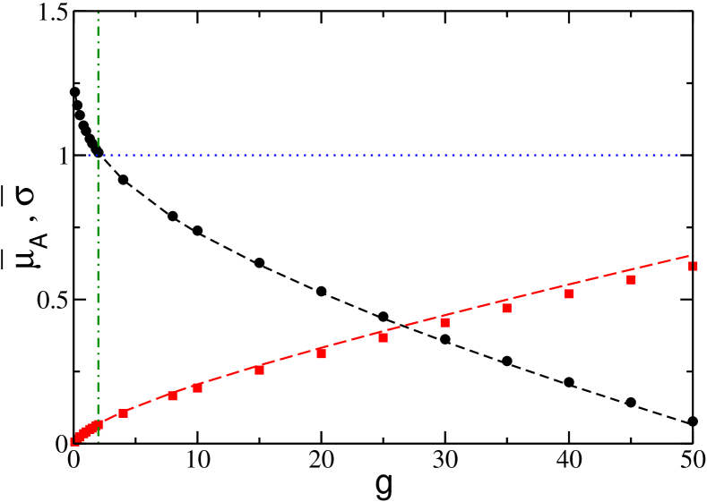
Figure 4: Effective average input of the active neurons ${\bar{\mu}_{A}}$ (black circles) and average fluctuations of the synaptic currents ${\bar{\sigma}}$ (red squares) as a function of the inhibitory coupling $g$. The threshold potential $\theta=1$ is marked by the (blue) horizontal dotted line and $g_{m}$ by the (green) vertical dash-dotted line. The dashed black (red) line refer to the theoretical estimation for $\mu_{A}$ ($\sigma$) reported in Eq. (4) (Eq. (10)) and averaged only over the active neurons. The data refer to $N=1400$, $K=140$, $[l_{1},l_{2}]=[1.0:1.5]$ and to a simulation time $t_{S}=1\times 10^{6}$.

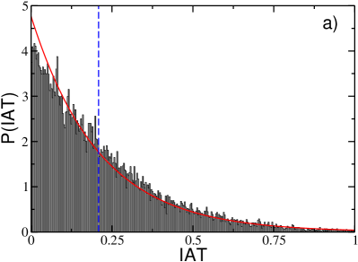
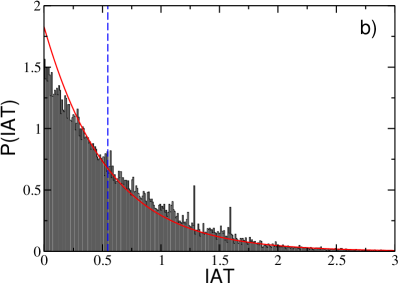
Figure 5: Probability distributions of the inter-arrival times (IATs) for a generic neuron in the network for a) $g=1.3$ and b) $g=10$. In both panels, the red continuous line indicate the exponential distribution corresponding to a purely Poissonian process with arrival rate given by $R=n_{A}K{\bar{\nu}}$ and the dashed blue vertical lines refer to the average IAT for the Poissonian distribution, namely $1/R$. The distributions have been evaluated for the arrival of $5\times 10^{5}$ IPSPs. Other parameters used for the simulation as in Fig. 1 (b).

For instantaneous IPSP, the current fluctuations are due to stable chaos politi2010stable , since the maximal Lyapunov exponent is negative for the whole range of coupling, as we have verified. Therefore, as reported by many authors, erratic fluctuations in inhibitory neural networks with instantaneous synapses are due to finite amplitude instabilities, while at the infinitesimal level the system is stable Zillmer2006 ; JhankeTimme2008PRL ; Timme2009ChaosBalance ; Luccioli2010Irregular ; MonteforteBalanced2012 ; angulo2014 ; ullner2016self .

In this picture, the silent neurons stay in a quiescent state corresponding to the minimum of the effective potential ${\cal U}(v)=v^{2}/2-\mu v$ and in order to fire they should overcome a barrier $\Delta{\cal U}=(\theta-\mu)^{2}/2$. The average time $t_{A}$ required to overcome such barrier can be estimated accordingly to the Kramers’ theory for activation processes hanggi1990reaction ; tuckwell2005 , namely

$$t_{A}\simeq\tau_{0}\exp\left({\frac{\left(\theta-\mu({I})\right)^{2}}{\sigma^{2}}}\right)\;;$$ (11)

where $\tau_{0}$ is an effective time scale taking in account the intrinsic non stationarity of the process, i.e. the fact that the number of active neurons increases during the time evolution.

It is important to stress that the expression (11) will remain valid also in the limit of large synaptic couplings, because not only $\sigma^{2}$, but also the barrier height will increase with $g$. Furthermore, both these quantities grow quadratically with $g$ at sufficiently large synaptic strength, as it can be inferred from Eqs. (4) and (10).

It is reasonable to assume that at a given time $t_{S}$ all neurons with $t_{A}<t_{S}$ will have fired at least once and that the more excitable will fire first. Therefore by assuming that the fraction of active neurons at time $t_{S}$ is $n_{A}(t_{S})$, the last neuron which has fired should be characterized by the following excitability

$$\hat{I}=l_{2}-n_{A}(t_{S})(l_{2}-l_{1})\;;$$ (12)

for excitabilities $I$ uniformly distributed in the interval $[l_{1},l_{2}]$. In order to obtain an explicit expression for the fraction of active neurons at time $t_{S}$, one should solve the equation (11) for the neuron with excitability $\hat{I}$ by setting $t_{S}=t_{A}$, thus obtaining the following solution

$$n_{A}(t_{S})=\left\{\begin{array}[]{lr}\dfrac{\phi-2\beta\gamma+\sqrt{\phi^{2}-4\phi\beta\gamma}}{2\gamma^{2}}&\mbox{if }n_{A}<1\\ 1&\text{otherwise}\end{array}\right.$$ (13)

where

$$\gamma=(l_{2}-l_{1})+g\bar{\nu}\quad\phi=\frac{g^{2}}{K}\bar{\nu}\ln(t_{S}/\tau_{0})\quad\beta=\theta-l_{2}\enskip.$$

Equation (13) gives the dependence of $n_{A}$ on the coupling strength $g$ for a fixed integration time $t_{S}$ and time scale $\tau_{0}$, whenever we can provide the value of the average frequency $\bar{\nu}$. A quick inspection to Eqs. (11) and (13) shows that, setting $n_{A}=1$, we obtain two solutions for the critical couplings $g_{c1}$ ($g_{c2}$) below (above) which all neurons will fire at least once in the cosidered time interval. The solutions are reported in Fig 6, in particular we observe that whenever $l_{1}\to v_{th}$ the critical coupling $g_{c1}$ will vanish, analogously to the fully coupled situation. These results clearly indicate that $n_{A}$ should display a minimum for some finite coupling strenght $g_{m}\in(g_{c1},g_{c2})$. Furthermore, as shown in Fig 6 the two critical couplings approach one another for increasing $t_{S}$ and finally merge, indicating that at sufficiently long times all the neurons will be active at any synaptic coupling strength $g$.

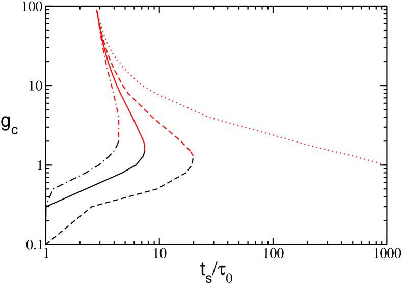
Figure 6: Critical values $g_{c1}$ (black) and $g_{c2}$ (red) as calculated from Eq. (13) for $l_{1}=1.2$ (dash-dotted), $l_{1}=1.15$ (continuous), $l_{1}=1.1$ (dashed) and $l_{1}=1.0$ (dotted line). All the values entering in Eq. (13) are taken from simulation. All other parameters used for the simulation as in Fig. 1 (b).

The average frequency $\bar{\nu}$ can be obtained analytically by following the approach described in Appendix B for LIF neurons with instantaneous synapses subject to inhibitory Poissonian spike trains. In particular, the self-consistent expression for the average frequency reads as

$$\bar{\nu}=\int_{\{I_{A}\}}dIP(I)\nu_{0}(I,G,n_{A},\bar{\nu})\quad;$$ (14)

where the explicit expression of $\nu_{0}$ is given by Eq. (31) in Appendix B.

The simultaneous solution of Eqs. (13) and (14) provides a theoretical estimation of $n_{A}$ and $\bar{\nu}$ for the whole considered range of synaptic strength, once the unknown time scale $\tau_{0}$ is fixed. This time scale has been determined via an optimal fitting procedure for sparse networks with $N=400$ and $K=20$, 40 and 80 at a fixed integration time $t_{S}=1\times 10^{6}$. The results for $n_{A}$ are reported in Fig. 7 (a), the estimated curves reproduce reasonably well the numerical data for $K=20$ and 40, while for $K=80$ the agreement worsens at large coupling strengths. This should be due to the fact that by increasing $g$ and $K$ the spike trains stimulating each neuron cannot be assumed to be completely independent, as done for the derivation of Eqs. (13) and (14). Nevertheless, the average frequency $\bar{\nu}$ is quantitatively well reproduced for the considered $K$ values over the entire range of the synaptic strengths, as it is evident from Figs. 7 (b-d). A more detailed comparison between the theoretical estimations and the numerical data can be obtained by considering the distributions $P(\nu)$ of the single neuron firing rate for different coupling strengths reported in Figs. 7 (k-m) for $K=40$. The overall agreement can be considered as more than satisfactory, the observable discrepancies are probably due to the fact that our approach neglect a further source of disorder present in the system and related to the heterogeneity in the number of active pre-synaptic neurons BrunelHakim1999 .

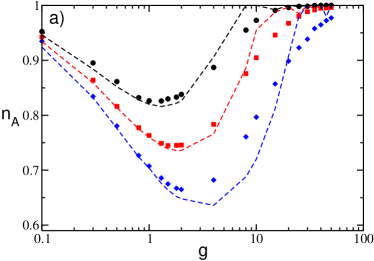
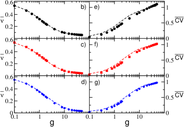
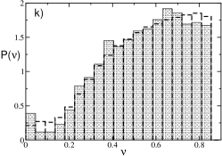
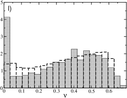
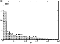
Figure 7: a) Fraction of active neurons $n_{A}$ as a function of inhibition for several values of $K$. b-d) Average network’s firing rate $\bar{\nu}$ for the same cases depicted in a), and the corresponding $\overline{CV}$ (e-f). In all panels, filled symbols correspond to numerical data and dashed lines to semi-analytic values: black circles correspond to $K=20$ ($t_{s}/\tau_{0}=11$), red squares to $K=40$ ($t_{s}/\tau_{0}=19$) and blue diamonds to $K=80$ ($t_{s}/\tau_{0}=26.6$). The data are averaged over a time interval $t_{S}=1\times 10^{6}$ and 10 different realizations of the random network. h-j) Raster plots for three different synaptic strengths for $N=400$ and $K=40$: namely, h) $g=0.1$; i) $g=1$ and j) $g=8$. The corresponding value for the fraction of active neurons, average frequency and average coefficient of variation are $n_{A}=(0.94,0.76,0.88)$, $\bar{\nu}=(0.55,0.34,0.10)$ and $\overline{CV}=(0.04,0.27,0.76)$, respectively. The neurons are ordered in terms of their intrinsic excitability and the time is rescaled by the average frequency $\bar{\nu}$. k-l) Probability distributions $P(\nu)$ of the the single neuron firing rate $\nu$, for the same values of $g$ in the panels above. Empty-discontinuous bars correspond to the theoretical prediction while the filled bars indicate the histogram calculated with the simulation. The remaining parameters as in Fig. 1 (b).

We have also estimated analytically the average coefficient of variation of the firing neurons $\overline{CV}$ by extending the method derived in richardson2010firing to obtain the response of a neuron receiving synaptic shot noise inputs. The analytic expressions of the coefficient of variation for LIF neurons subject to inhibitory shot noise with fixed post-synaptic amplitude are obtained by estimating the second moment of the associated first-passage-time distribution, the details are reported in Appendix C. The coefficient of variation can be estimated, once the self consistent values for $n_{A}$ and $\bar{\nu}$ have been obtained via Eqs. (13) and (14). The comparison with the numerical data, reported in Figs 7 (e-g), reveals a good agreement over the whole range of synaptic strengths for all the considered in-degrees.

At sufficiently small synaptic coupling the neurons fire tonically and almost independently, as it emerges clearly from the raster plot in Fig 7 (h) and by the fact that $\bar{\nu}$ approaches the average value for the uncoupled system (namely, $0.605$) and $\overline{CV}\to 0$. Furthermore, the neuronal firing rates are distributed towards finite values indicating that the inhibition as a minor role in this case, as shown in Fig 7 (k). By increasing the coupling, $n_{A}$ decreases, as an effect of the inhibition more and more neurons are silenced (as evident from Fig.  7 (l)) and the average firing rate decrease, at the same time the dynamics becomes slightly more irregular as shown in Fig 7 (i). At large coupling $g>g_{m}$, a new regime appears, where almost all neurons become active but with an extremely slow dynamics which is essentially stochastic with $\overline{CV}\simeq 1$, as testified also by the raster plot reported in Fig 7 (j) and by by the firing rate distribution shown in Fig 7 (m).

Furthermore, from Fig. 7(a) it is clear that the value of the minimum of the fraction of active neurons ${n_{A}}_{m}$ decreases by increasing the network in-degree $K$, while $g_{m}$ increases with $K$. This behaviour is further investigated in a larger network, namely $N=1400$, and reported in the inset of Fig. 8. It is evident that $n_{A}$ stays close to the globally coupled solutions over larger and larger intervals for increasing $K$. This can be qualitatively understood by the fact that the current fluctuations Eq. (10), responsible for the rebirth of silent neurons, are proportional to $g$ and scales as $1/\sqrt{K}$, therefore at larger in-degree the fluctuations have similar intensities only for larger synaptic coupling.

The general mechanism behind neurons’ rebirth can be understood by considering the value of the effective neuronal input and of the current fluctuations as a function of $g$. As shown in Fig. 4, the effective input current $\bar{\mu}_{A}$, averaged over the active neurons, essentially coincide with the average of the excitability ${\bar{I}}_{A}$ for $g\to 0$, where the neurons can be considered as independent one from the others. The inhibition leads to a decrease of ${\bar{\mu}}_{A}$, and to a crossing of the threshold $\theta$ exactly at $g=g_{m}$. This indicates that at $g<g_{m}$ the active neurons, being on average supra-threshold, fire almost tonically inhibiting the losers via a WTA mechanism. In this case the firing neurons are essentially mean-driven and the current fluctuations play a role on the rebirth of silent neurons only on extremely long time scales, this is confirmed by the low values of $\bar{\sigma}$ in such a range, as evident from Fig. 4. On the other hand, for $g>g_{m}$, the active neurons are now on average below threshold while the fluctuations dominate the dynamics. In particular, the firing is now extremely irregular being due mainly to reactivation processes. Therefore the origin of the minimum in $n_{A}$ can be understood as a transition from a mean-driven to a fluctuation-driven regime renart2007 .

A quantitative definition of $g_{m}$ can be given by requiring that the average input current of the active neurons $\bar{\mu}_{A}$ crosses the threshold $\theta$ at $g=g_{m}$, namely

$$\bar{\mu}_{A}(g_{m})=\bar{I}_{A}-g_{m}\bar{\nu}_{m}{n_{A}}_{m}=\theta\;;$$

where $\bar{I}_{A}$ is the average excitability of the firing neurons, while ${n_{A}}_{m}$ and $\bar{\nu}_{m}$ are the number of active neurons and the average frequency at the minimum.

For an uniform distribution $P(I)$, a simpler expression for $g_{m}$ can be derived, namely

$$g_{m}=\bar{\nu}^{-1}_{m}\left[\frac{l_{2}-\theta}{n_{A_{m}}}+\frac{1}{2}(l_{1}-l_{2})\right]\;.$$ (15)

We have compared the numerical measurements of $g_{m}$ with the estimations obtained by employing Eq. (15), where $n_{A_{m}}$ and $\bar{\nu}$ are obtained from the simulations. As shown in Fig. 8 for a network of size $N=1,400$, the overall agreement is more than satisfactory for in-degrees ranging over almost two decades (namely, for $20\leq K\leq 600$). This confirms that our guess (that the minimum $n_{A_{m}}$ occurs exactly at the transition from mean-driven to fluctuation-driven dynamics) is consistent with the numerical data for a wide range of in-degrees.

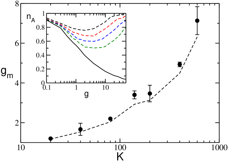
Figure 8: $g_{m}$ as a function of the in-degree $K$. The symbols refer to numerical data, while the dashed line to the expression (15). Inset: $n_{A}$ versus $g$ for the fully coupled case (solid black line) and for diluted networks (dashed lines), from top to bottom $K=20$, 40, 80, 140. A network of size $N=1400$ is evolved during a period $t_{S}=1\times 10^{5}$ after discarding a transient of $10^{6}$ spikes, the data are averaged over 5 different random realizations of the network. Other parameters as in Fig. 1.

It should be stressed that, as we have verified for various system sizes (namely, $N=700$,1400 and 2800) and for a constant average in-degree $K=140$, for instantaneous synapses the network is in an heterogeneous asynchronous state for all the considered values of the synaptic coupling. This is demonstrated by the fact that the intensity of the fluctuations of the average firing activity, measured by considering the low-pass filtered linear super-position of all the spikes emitted in the network, vanishes as $1/\sqrt{N}$ wang1996gamma . Therefore, the observed transition at $g=g_{m}$ is not associated to the emergence of irregular collective behaviours as reported for globally coupled heterogeneous inhibitory networks of LIF neurons with delay Luccioli2010Irregular and of pulse-coupled phase oscillators ullner2016self .

V Effect of synaptic filtering

In this Section we will investigate how synaptic filtering can influence the previously reported results. In particular, we will consider non instantaneous IPSP with $\alpha$-function profile (3), whose evolution is ruled by a single time scale $\tau_{\alpha}$.

V.1 Fully Coupled Networks

Let us first examine the fully coupled topology, in this case we observe analogously to the $\delta$-pulse coupling that by increasing the inhibition, the number of active neurons steadily decreases towards a limit where only few neurons (or eventually only one) will survive. At the same time the average frequency also decreases monotonically, as shown in Fig. 9 for two different $\tau_{\alpha}$ differing by almost two orders of magnitude. Furthermore, the mean field estimations (7) and (8) obtained for $n_{A}$ and $\bar{\nu}$ represent a very good approximation also for $\alpha$-pulses (as shown in Fig. 9). In particular, the mean field estimation essentially coincides with the numerical values for slow synapses, as evident from the data reported in Fig. 9 for $\tau_{\alpha}=10$ (black filled circles). This can be explained by the fact that for sufficiently slow synapses, with $\tau_{P}>{\bar{T}}_{ISI}$, the neurons feel the synaptic input current as continuous, because each input pulse has essentially no time to decay between two firing events. Therefore the mean field approximation for the input current (4) works definitely well in this case. This is particularly true for $\tau_{\alpha}=10$, where $\tau_{P}=20$ and ${\bar{T}}_{ISI}\simeq 2-6$ in the range of the considered coupling. While for $\tau_{\alpha}=0.125$, we observe some deviation from the mean field results (red squares in Fig. 9) and the reason for these discrepancies reside in the fact that $\tau_{P}<{\bar{T}}_{ISI}$ for any coupling strength, therefore the discreteness of the pulses cannot be completely neglected in particular for large amplitudes (large synaptic couplings) analogously to what observed for instantaneous synapses.

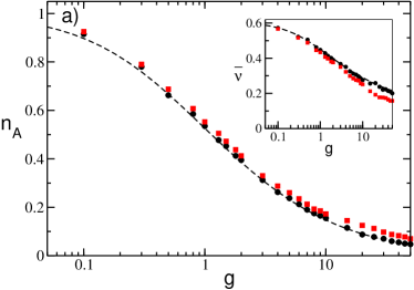
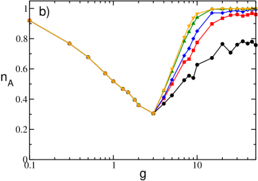
Figure 9: Fraction of active neurons $n_{A}$ as a function of the inhibition with IPSPs with $\alpha$-profile for a fully coupled topology (a) and a sparse network (b) with $K=20$. a) Black (red) symbols correspond to $\tau_{\alpha}=10$ ($\tau_{\alpha}=0.125$), while the dashed lines are the theoretical predictions (7) and (8) previously reported for instantaneous synapses. The data are averaged over a time window $t_{S}=1\times 10^{5}$. Inset: average frequency $\bar{\nu}$ as a function of $g$. b) $n_{A}$ is measured at successive times : from lower to upper curve the considered times are $t_{S}=\{1000,\,5000,\,10000,\,50000,\,100000\}$, while $\tau_{\alpha}=10$. The system size is $N=400$ in both cases, the distribution of excitabilities is uniform with $[l_{1},l_{2}]=[1.0,1.5]$ and $\theta=1$.

V.2 Sparse Networks

For the sparse networks $n_{A}$ has the same qualitative behaviour as a function of the synaptic inhibition observed for instantaneous IPSPs, as shown in Fig. 9 (b) and Fig. 10 (a). The value of $n_{A}$ decreases with $g$ and reaches a minimal value at $g_{m}$, afterwards it increases towards $n_{A}=1$ at larger coupling. The origin of the minimum of $n_{A}$ as a function of $g$ is the same as for instantaneous synapses, for $g<g_{m}$ the active neurons are subject on average to a supra-threshold effective input ${\bar{\mu}}_{A}$, while at larger coupling ${\bar{\mu}}_{A}<\theta$, as shown in the inset of Fig. 10 (b). This is true for any value of $\tau_{\alpha}$, however, this transition from mean- to fluctuation-driven becomes dramatic for slow synapses . As evidenced from the data for the average output firing rate $\bar{\nu}$ and the average coefficient of variation $\overline{CV}$, these quantities have almost discontinuous jumps at $g=g_{m}$, as shown in Fig. 11 .

Therefore, let us first concentrate on slow synapses with $\tau_{\alpha}$ larger than the membrane time constant, which is one for adimensional units. For $g<g_{m}$ the fraction of active neurons is frozen in time, at least on the considered time scales, as revealed by the data in Fig. 9 (b). Furthermore, for $g<g_{m}$, the mean field approximation obtained for the fully coupled case works almost perfectly both for $n_{A}$ and ${\bar{\nu}}$, as reported in Fig. 10 (a). The frozen phase is characterized by extremely small values of the current fluctuations ${\bar{\sigma}}$ (as shown Fig. 10 (b)) and a quite high firing rate ${\bar{\nu}}\simeq 0.4-0.5$ with an associated average coefficient of variation $\overline{CV}$ almost zero (see black circles and red squares in Fig. 11). Instead, for $g>g_{m}$ the number of active neurons increases in time similarly to what observed for the instantaneous synapses, while the average frequency becomes extremely small $\bar{\nu}\simeq 0.04-0.09$ and the value of the coefficient of variation becomes definitely larger than one.

These effects can be explained by the fact that, below $g_{m}$ the active neurons (the winners) are subject to an effective input ${\bar{\mu}}_{A}>\theta$ that induces a quite regular firing, as testified by the raster plot displayed in Fig. 10 (c). The supra-threshold activity of the winners joined together with the filtering action of the synapses guarantee that on average each neuron in the network receive an almost continuous current, with small fluctuations in time. These results explain why the mean field approximation still works in the frozen phase, where the fluctuations in the synaptic currents are essentially negligible and unable to induce any neuron’s rebirth, at least on realistic time scales. In this regime the only mechanism in action is the WTA, fluctuations begin to have a role for slow synapses only for $g>g_{m}$. Indeed, as shown in Fig. 10 (b), the synaptic fluctuations $\bar{\sigma}$ for $\tau_{\alpha}=10$ (black circles) are almost negligible for $g<g_{m}$ and show an enormous increase at $g=g_{m}$ of almost two orders of magnitude. Similarly at $\tau_{\alpha}=2$ (red square) a noticeable increase of ${\bar{\sigma}}$ is observable at the transition.

In order to better understand the abrupt changes in $\bar{\nu}$ and in $\overline{CV}$ observable for slow synapses at $g=g_{m}$, let us consider the case $\tau_{\alpha}=10$. As shown in Fig. 11 (c), $\tau_{P}>{\bar{T}}_{ISI}\simeq 2-3$ for $g<g_{m}$, therefore for these couplings the IPSPs have no time to decay between a firing emission and the next one, thus the synaptic fluctuations $\bar{\sigma}$ are definitely small in this case, as already shown. At $g_{m}$ an abrupt jump is observable to large values ${\bar{T}}_{ISI}>\tau_{P}$, this is due to the fact that now the neurons display bursting activities, as evident from the raster plot shown in Fig. 10 (d). The bursting is due to the fact that, for $g>g_{m}$, the active neurons are subject to an effective input which is on average sub-threshold, therefore the neurons preferentially tend to be silent. However, due to current fluctuations a neuron can pass the threshold and the silent periods can be interrupted by bursting phases where the neuron fires almost regularly. As a matter of fact, the silent (inter-burst) periods are very long $\simeq 700-900$, if compared to the duration of the bursting periods, namely $\simeq 25-50$, as shown in Fig. 11 (c). This explains the abrupt decrease of the average firing rate reported in Fig. 11 (a). Furthermore, the inter-burst periods are exponentially distributed with an associated coefficient of variation $\simeq 0.8-1.0$, which clearly indicates the stochastic nature of the switching from the silent to the bursting phase. The firing periods within the bursting phase are instead quite regular, with an associated coefficient of variation $\simeq 0.2$, and with a duration similar to ${\bar{T}}_{ISI}$ measured in the frozen phase (shaded gray circles in Fig. 11 (c)). Therefore, above $g_{m}$ the distribution of the ISI exhibits a long exponential tail associated to the bursting activity and this explains the very large values of the measured coefficient of variation. By increasing the coupling the fluctuations in the input current becomes larger thus the fraction of neurons that fires at least once within a certain time interval increases. At the same time, $\bar{\nu}$, the average inter-burst periods and the firing periods within the bursting phase remain almost constant at $g>10$, as shown in Fig. 11 (a). This indicates that the decrease of ${\bar{\mu}}_{A}$ and the increase of $\bar{\sigma}$ due to the increased inhibitory coupling essentially compensate each other in this range. Indeed, we have verified that for $\tau_{\alpha}=10$ and $\tau_{\alpha}=2$ ${\bar{\mu}}_{A}$ ($\bar{\sigma}$) decreases (increases) linearly with $g$ with similar slopes, namely ${\bar{\mu}}_{A}\simeq 0.88-0.029g$ while $\bar{\sigma}\simeq 0.05+0.023g$.

For faster synapses, the frozen phase is no more present. Furthermore, due to rebirths induced by current flutuations, $n_{A}$ is always larger than the fully coupled mean field result (8), even at $g<g_{m}$. It is interesting to notice that by decreasing $\tau_{\alpha}$, we are now approaching the instantaneous limit, as indicated by the results reported for $n_{A}$ in Fig. 10 (a) and $\overline{CV}$ in Fig. 11 (b). In particular, for $\tau_{\alpha}=0.125$ (green triangles) the data almost collapse on the corresponding values measured for instantaneous synapses in a sparse networks with the same characteristics and over a similar time interval (dashed line). Furthermore, for fast synapses with $\tau_{\alpha}<1$ the bursting activity is no more present as it can be appreciated by the fact that at most $\overline{CV}$ approaches one in the very large coupling limit.

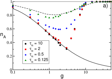
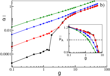
Figure 10: a) Fraction of active neurons for a network of $\alpha$-pulse coupled neurons as a function of $g$ for various $\tau_{\alpha}$: namely, $\tau_{\alpha}=10$ (black circles), $\tau_{\alpha}=2$ (red squares), $\tau_{\alpha}=0.5$ (blue diamonds) and $\tau_{\alpha}=0.125$ (green triangles). For instantaneous synapses, the fully coupled analytic solution is reported (solid line), as well as the measured $n_{A}$ for the sparse network with same level of dilution and estimated over the same time interval (dashed line). b) Average fluctuations of the synaptic current ${\bar{\sigma}}$ versus $g$ for ISPS with $\alpha$-profile the symbols refer to the same $\tau_{\alpha}$ as in panel (a). Inset: Average input current ${\bar{\mu}}_{A}$ of the active neurons vs $g$, the dashed line is the threshold value $\theta=1$. The simulation time has been fixed to $t_{S}=1\times 10^{5}$. c-d) Raster plots for two different synaptic strengths for $\tau_{\alpha}=10$: namely, c) $g=1$ corresponds to $n_{A}\simeq 0.52$, $\bar{\nu}\simeq 0.45$ and $\overline{CV}\simeq 3\times 10^{-4}$; while i) $g=10$ to $n_{A}\simeq 0.99$, $\bar{\nu}\simeq 0.06$ and $\overline{CV}\simeq 4.1$. The neurons are ordered according to their intrinsic excitability and the time is rescaled by the average frequency $\bar{\nu}$. The data have been obtained for a system size $N=400$ and $K=20$, other parameters as in Fig. 9.

For sufficiently slow synapses, the average firing rate $\bar{\nu}$ can be estimated analytically by applying the so-called adiabatic approach developed by Moreno-Bote and Parga in moreno2004 ; moreno2010response . This method applies to LIF neurons with a synaptic time scale definitely longer than the membrane time constant. In these conditions, the output firing rate can be reproduced by assuming that the neuron is subject to an input current with time correlated fluctuations, which can be represented as colored noise with a correlation time given by the pulse duration $\tau_{P}=2\tau_{\alpha}$ (for more details see Appendix D). In this case we are unable to develop a self-consistent approach to obtain at the same time $n_{A}$ and the average frequency. However, once $n_{A}$ is provided by simulations the analytic estimated (45) obtained with the adiabatic approach gives very good agreement with the numerical data for sufficiently slow synapses, namely for $\tau_{P}\geq 1$, as shown in Fig. 11(a) for $\tau_{\alpha}=10$, 2 and 0.5. The theoretical expression (45) is even able to reproduce the jump in the average frequencies observable at $g_{m}$ and therefore to capture the bursting phenomenon. By considering $\tau_{P}<1$, as expected, the theoretical expression fails to reproduce the numerical data in particular at large coupling (see the dashed green line in Fig. 11(a) corresponding to $\tau_{\alpha}=0.125$).

By following the arguments reported in moreno2004 , the bursting phenomenon observed for $\tau_{\alpha}>1$ and $g>g_{m}$ can be interpreted at a mean field level as the response of a sub-threshold LIF neuron subject to colored noise with correlation $\tau_{P}$. In this case, the neuron is definitely sub-threshold, but in presence of a large fluctuation it can be lead to fire and due to the finite correlation time it can remain supra-threshold regularly firing for a period $\simeq\tau_{P}$. The validity of this interpretation is confirmed by the fact that the measured average bursting periods are of the order of the correlation time $\tau_{P}=2\tau_{\alpha}$, namely, $\simeq 27-50$ ($\simeq 7-14$) for $\tau_{\alpha}=10$ ($\tau_{\alpha}=2$).

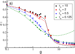
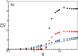
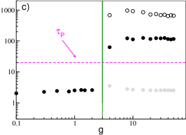
Figure 11: a) Average firing rate $\bar{\nu}$ vs $g$ for a network of $\alpha$-pulse coupled neurons, for four values of $\tau_{\alpha}$. Theoretical estimations for $\bar{\nu}$ calculated with the adiabatic approach (45) are reported as dashed lines of colors corresponding to the relative symbols. b) Average coefficient of variation $\overline{CV}$ for four values of $\tau_{\alpha}$ as a function of the inhibition. The dashed line refers to the values obtained for instantaneous synapses and a sparse network with the same value of dilution. c): Average inter-spike interval ${\bar{T}}_{ISI}$ (filled black circles) as a function of $g$ for $\tau_{\alpha}=10$. For $g>g_{m}$ the average inter-burst interval (empty circles) and the average ISI measured within bursts (gray circles) are also shown, together with the position of $g_{m}$ (green veritical line). The symbols and colors denote the same $\tau_{\alpha}$ values as in Fig. 10. All the reported data were calculated for a system size $N=400$ and $K=20$ and for a fixed simulation time of $t_{S}=1\times 10^{5}$.

As a final point, to better understand the dynamical origin of the measured fluctuations in this deterministic model, we have estimated the maximal Lyapunov exponent $\lambda$. As expected from previous analysis, for non-instantaneous synapses we can observe the emergence of regular chaos in purely inhibitory networks  Timme2009ChaosBalance ; Zillmer2009LongTrans ; angulo2015Striatum . In particular, for sufficiently fast synapses, we typically note a transition from a chaotic state at low coupling to a linearly stable regime (with $\lambda<0$) at large synaptic strengths, as shown in Fig. 12 (a) for $\tau_{\alpha}=0.125$. Despite the fact that current fluctuations are monotonically increasing with the synaptic strength. Therefore, fluctuations are due to chaos, at small coupling, while at larger $g$ they are due to finite amplitude instabilities, as expected for stable chaotic systems angulo2014 . However, the passage from positive to negative values of the maximal Lyapunov exponent is not related to the transition occurring at $g_{m}$ from a mean-driven to a fluctuation-driven dynamics in the network.

For slow synapses, $\lambda$ is essentially zero at small coupling in the frozen phase characterized by tonic spiking of the neurons, while it becomes positive by approaching $g_{m}$. For larger synaptic strengths $\lambda$, after reaching a maximal value, decreases and it can become eventually negative at $g>>g_{m}$, as reported in Fig. 12 (b-c). Only for extremely slow synapses, as shown in Fig. 12 (c) for $\tau_{\alpha}=10$, the chaos onset seems to coincide with the transition occurring at $g_{m}$. These findings are consistent with recent results concerning the emergence of asynchronous rate chaos in homogeneous inhibitory LIF networks with deterministic harish2015 and stochastic kadmon2015 evolution. However, a detailed analysis of this aspect goes beyond the scope of the present paper.

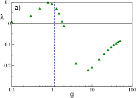
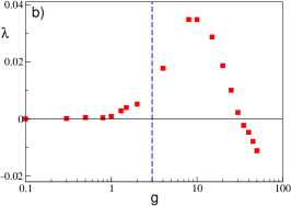
Figure 12: Maximal Lyapunov exponent $\lambda$ versus $g$ for a network of $\alpha$-pulse coupled neurons, for $\tau_{\alpha}=0.125$ (a), $\tau_{\alpha}=2$ (b) and $\tau_{\alpha}=10$ (c). The blue dashed vertical line denote the $g_{m}$ value. All the reported data were calculated for a system size $N=400$ and $K=20$ and for simulation times $5\times 10^{4}\leq t_{S}\leq 7\times 10^{5}$ ensuring a good convergence of $\lambda$ to its asymptotic value. The other parameters are as in Fig. 9.

VI Discussion

In this paper we have shown that the effect reported in ponzi2013optimal ; angulo2015Striatum is observable whenever two sources of quenched disorder are present in the network: namely, a random distribution of the neural properties and a random topology. In particular, we have shown that neuron’s death due to synaptic inhibition is observable only for heterogeneous distributions of the neural excitabilities. Furthermore, in a globally coupled network the less excitable neurons are silenced for increasing synaptic strength until only one or few neurons remain active. This scenario corresponds to the winner-takes-all mechanism via lateral inhibition, which has been often invoked in neuroscience to explain several brain functions yuille1989 . WTA mechanisms have been proposed to model hippocampal CA1 activity coultrip1992cortical , as well as to be at the basis of visual velocity estimate grzywacz1990 , and to be essential for controlling visual attention itti2001 .

However, most brain circuits are characterized by sparse connectivity laughlin2003communication ; plenz2003 ; bullmore2009 , in these networks we have shown that an increase in inhibition can lead from a phase dominated by neuronal death to a regime where neuronal rebirths take place. Therefore the growth of inhibition can have the counter-intuitive effect to activate silent neurons due to the enhancement of current fluctuations. The reported transition is characterized by a passage from a regime dominated by the almost tonic activity of a group of neurons, to a phase where sub-threshold fluctuations are at the origin of the irregular firing of large part of the neurons in the network. For instantaneous synapses, the average first and second moment of the firing distributions have been obtained together with the fraction of active neurons within a mean-field approach, where the neuronal rebirth is interpreted as an activation process driven by synaptic shot noise richardson2010firing .

For a finite synaptic time smaller than the characteristic membrane time constant, the scenario is similar to the one observed for instantaneous synapses. However, the transition from mean-driven to fluctuation-driven dynamics becomes dramatic for sufficiently slow synapses. In this situation one observes for low synaptic strength a frozen phase, where the synaptic filtering washes out the current fluctuations leading to an extremely regular dynamics controlled only by a WTA mechanism. As soon as the inhibition is sufficiently strong to lead the active neurons below threshold, the neuronal activity becomes extremely irregular exhibiting long silent phases interrupted by bursting events. The origin of these bursting periods can be understood in terms of the emergence of correlations in the current fluctuations induced by the slow synaptic timescale, as explained in moreno2004 .

In our model, the random dilution of the network connectivity is a fundamental ingredient to generate current fluctuations, whose intensity is controlled by the average network in-degree $K$. A natural question is whether the reported scenario will be still observable in the thermodynamic limit. On the basis of previous studies we can affirm that this depends on how $K$ scales with the system size golomb2001 ; Tattini2011Coherent ; Luccioli2012PRL . In particular, if $K$ stays finite for $N\to\infty$ the transition will still be observable. For $K$ diverging with $N$, the fluctuations become negligible for sufficiently large system sizes, impeding neuronal rebirths and the dynamics will be controlled only by the WTA mechanism.

An additional source of randomness present in the network is related to the variability in the number of active pre-synaptic neurons. In our mean-field approach we have assumed that each neuron is subject to $n_{A}K$ spike trains, however this is true only on average. The number of active pre-synaptic neurons is a random variable binomially distributed with average $n_{A}K$ and variance $n_{A}(1-n_{A})K$. Future developments of the theoretical approach here reported should include also such variability in the modeling of the network dynamics BrunelHakim1999 .

$\tau_{\alpha}/\tau_{m}$	$\tau_{m}$ (msec)	Spike Rate (Hz)	$\overline{CV}$	Burst Duration (msec)	Spike Rate within Bursts (Hz)
$2$	$10$	4-6	$\simeq 1.8$	$100\pm 40$	$42\pm 2$
	$20$	2-3	$\simeq 1.8$	$200\pm 80$	$21\pm 1$
$10$	$10$	4-6	$\simeq 4.2$	$400\pm 150$	$41\pm 2$
	$20$	2-3	$\simeq 4.2$	$800\pm 300$	$20\pm 1$
	Experimental data	2-3	$\simeq 1.5-3$	$500-1100$	$31\pm 15$

Table 1: Comparison between the results obtained for slow $\alpha$- synapses and experimental data for MSNs.The numerical data refer to results obtained in the bursting phase, namely for synaptic strenght $g$ in the range $[10:50]$, for simulation times $t_{S}=1\times 10^{5}$, $N=400$ and $K=20$. The experimental data refer to MSNs population in striatum for free behaving wild type mice, data taken from miller2008dysregulated .

As a further aspect, we show that the considered model is not chaotic for instantaneous synapses, in such a case we observe irregular asynchronous states due to stable chaos politi2010stable . The system can become truly chaotic only for finite synaptic times Timme2009ChaosBalance ; angulo2014 . However, we report clear indications that for synapses faster than the membrane time constant $\tau_{m}$ the passage from mean-driven to fluctuation-driven dynamics is not related to the onset of chaos. Only for extremely slow synapses we have numerical evidences that the appearance of the bursting regime could be related to a passage from a zero Lyapunov exponent to a positive one, in agreement with the results reported in kadmon2015 ; harish2015 for homogeneous inhibitory networks. These preliminary indications demand for future, more detailed investigations of deterministic spiking networks in order to relate fluctuation-driven regime and chaos onsets. Moreover, we expect that it will be hard to distinguish whether the erratic current fluctuations are due to regular chaos or stable chaos on the basis of the analysis of the network activity, as also pointed out in Timme2009ChaosBalance .

For what concerns the biological relevance of the presented model, we can attempt a comparison with experimental data obtained for MSNs in the striatum. This population of neurons is fully inhibitory with sparse lateral connections (connection probability $\simeq 10-20\%$ tunstall2002inhibitory ; taverna2004sparseStriatum ), unidirectional and relatively weak tepper2004gabaergic . Furthermore, for MSNs within the same collateral network the axonal propagation delays are quite small $\simeq 1-2$ ms taverna2008 and they can be safely neglected. The dynamics of these neurons in behaving mice, reveals a low average firing rate with irregular firing activity (bursting) with associated large coefficient of variation miller2008dysregulated . As we have shown, these features can be reproduced by sparse networks of LIF neurons with sufficiently slow synapses at $g>g_{m}$ and $\tau_{\alpha}>\tau_{m}$. For values of the membrane time constant which are comparable to the ones measured for MSNs plenz1998up ; planert2013membrane (namely, $\tau_{m}\simeq 10-20$ msec), the model is able to capture even quantitatively some of the main aspects of the MSNs dynamics, as shown in Table 1. We obtain a reasonable agreement with the experiments for sufficiently slow synapses, where the interaction among MSNs is mainly mediated by GABA_A receptors, which are characterized by IPSP durations of the order of $\simeq 5-20$ ms tunstall2002inhibitory ; koos2004comparison . However, apart the burst duration, which is definitely shorter, all the other aspects of the MSN dynamics can be already captured for $\tau_{\alpha}=2\tau_{m}$ (with $\tau_{m}=10$ ms) as shown in Table 1. Therefore, we can safely affirm, as also suggested in ponzi2013optimal , that the fluctuation driven regime emerging at $g>g_{m}$ is the most appropriate in order to reproduce the dynamical evolution of this population of neurons.

Other inhibitory populations are present in the basal ganglia. In particular two coexisting inhibitory populations, arkypallidal (Arkys) and prototypical (Protos) neurons, have been recently discovered in the external globus pallidus mallet2012dichotomous . These populations have distinct physiological and dynamical characteristics and have been shown to be fundamental for action suppression during the performance of behavioural tasks in rodents mallet2016arkypallidal . Protos are characterized by a high firing rate $\simeq 47$ Hz and a not too large coefficient of variation (namely, $CV\simeq 0.58$) both in awake and slow wave sleep (SWS) states, while Arkys have a clear bursting dynamics with $CV\simeq 1.9$ mallet2016arkypallidal ; dodson2015distinct . Furthermore, the firing rate of Arkys is definitely larger in the awake state (namely, $\simeq 9$ Hz) with respect to the SWS state, where the firing rates are $\simeq 3-5$ Hz mallet2016arkypallidal .

On the basis of our results, on the one hand Protos can be modeled as LIF neurons with reasonable fast synapses in a mean driven regime, namely with a synaptic coupling $g<g_{m}$. On the other hand, Arkys should be characterized by IPSP with definitely longer duration and they should be in a fluctuation driven phase as suggested from the results reported in Fig. 11. Since, as shown in Fig. 11 (a), the firing rate of inhibitory neurons decrease by increasing the synaptic strenght $g$ we expect that the passage from awake to slow wave sleep should be characterized by a reinforcement of Arkys synapses. Our conjectures about Arkys and Protos synaptic properties based on their dynamical behaviours ask for for experimental verification, which we hope will happen shortly.

Besides the straightforward applicability of our findings to networks of pulse-coupled oscillators mirollo1990synchronization , it has been recently shown that LIF networks with instantaneous and non-instantaneous synapses can be transformed into the Kuramoto-Daido model politi2015 ; daido1996 ; kuramotobook . Therefore, we expect that our findings should extend to phase oscillator arrays with repulsive coupling tsimring2005 . This will allow for a wider applicability of our results, due to the relevance of limit-cycle oscillators not only for modeling biological systems winfree2001 , but also for the many scientific and technological applications strogatz2001 ; dorfler2014 ; pikovsky2015 ; rodrigues2016 .

APPENDIX A: Event Driven Maps

By following Zillmer2007 ; Olmi2014linear the ordinary differential equations (1) and (2) describing the evolution of the membrane potential of the neurons can be rewritten exactly as discrete time maps connecting successive firing events occurring in the network. In the following we will report explicitly such event driven maps for the case of instantaneous and $\alpha$ synapses.

For instantaneous PSPs, the event-driven map for neuron $i$ takes the following expression:

$$v_{i}(n+1)=v_{i}(n)\text{e}^{-T_{\delta}}+I_{i}(1-\text{e}^{-T_{\delta}})-\frac{g}{K}C_{mi}\;,$$ (16)

where the sequence of firing times $\{t_{n}\}$ in the network is denoted by the integer indices $\{n\}$, $m$ is the index of the neuron firing at time $t_{n+1}$ and $T_{\delta}\equiv t_{n+1}-t_{n}$ is the inter-spike interval associated with two successive neuronal firing. This latter quantity is calculated from the following expression:

$$T_{\delta}=\log\left[\frac{I_{m}-v_{m}}{I_{m}-1}\right]\;.$$ (17)

For $\alpha$-pulses, the evolution of the synaptic current $E_{i}(t)$, stimulating the $i$-th neuron can be expressed in terms of a second order differential equation, namely

$$\ddot{E}_{i}(t)+2\alpha\dot{E}_{i}(t)+\alpha^{2}E_{i}(t)=\frac{\alpha^{2}}{K}\sum_{j\neq i}\sum_{n|t_{n}<t}C_{ij}\delta(t-t_{n})\qquad.$$ (18)

Eq. (18) can be rewritten as two first order differential equations by introducing the auxiliary variable $Q\equiv\dot{E}_{i}-\alpha E_{i}$, namely

$$\dot{E_{i}}=Q_{i}-\alpha E_{i},\quad\dot{Q_{i}}=-\alpha Q_{i}+\frac{\alpha^{2}}{K}\sum_{n|t_{n}<t}C_{ij}\delta(t-t_{n})$$ (19)

Finally, the equations (1) and (19) can be exactly integrated from the time $t_{n}$, just after the deliver of the $n$-th pulse, to time $t_{n+1}$ corresponding to the emission of the $(n+1)$-th spike, to obtain the following event driven map:

$$Q_{i}(n+1) =Q_{i}(n){\rm e}^{-\alpha T_{\alpha}}+\frac{\alpha^{2}}{K}C_{mi}$$ (20a)

$$E_{i}(n+1) =E_{i}(n){\rm e}^{-\alpha T_{\alpha}}+Q_{i}(n)T_{\alpha}{\rm e}^{-\alpha T_{\alpha}}$$ (20b)

$$v_{i}(n+1) =v_{i}(n){\rm e}^{-T_{\alpha}}+I_{i}(1-{\rm e}^{-T_{\alpha}})-gH_{i}(n)\,,$$ (20c)

In this case, the inter-spike interval $T_{\alpha}\equiv t_{n+1}-t_{n}$ should be estimated by solving self-consistently the following expression

$$T_{\alpha}=\ln\left[\frac{I_{m}-v_{m}(n)}{I_{m}-gH_{m}(n)-1}\right]\ ,$$ (21)

where the explicit expression for $H_{i}(n)$ appearing in equations (20c) and (21) is

$$H_{i}(n) = \frac{{\rm e}^{-T_{\alpha}}-{\rm e}^{-\alpha T_{\alpha}}}{\alpha-1}\left(E_{i}(n)+\frac{Q_{i}(n)}{\alpha-1}\right)$$ (22)

$$- \frac{T_{\alpha}{\rm e}^{-\alpha T_{\alpha}}}{\alpha-1}Q_{i}(n)\,.$$

The model so far introduced contains only adimensional units, however, the evolution equation for the membrane potential (1) can be easily re-expressed in terms of dimensional variables as follows

$$\tau_{m}\dot{V}_{i}(\tilde{t})={\tilde{I}}_{i}-{V}_{j}(\tilde{t})-\tau_{m}{\tilde{g}}{\tilde{E}}_{i}(\tilde{t})\quad i=1,\cdots,N\quad;$$ (23)

where we have chosen $\tau_{m}=10$ ms as the membrane time constant, ${\tilde{I}_{i}}$ represents the neural excitability and the external stimulations. Furthermore, ${\tilde{t}}=t\cdot\tau_{m}$, the field ${\tilde{E}}_{i}=E_{i}/\tau_{m}$ has the dimensionality of a frequency and ${\tilde{g}}$ of a voltage. The currents $\{{\tilde{I}}_{i}\}$ have also the dimensionality of a voltage, since they include the membrane resistance.

For the other parameters/variables the transformation to physical units is simply given by

$${V}_{i} = {V}_{r}+({V}_{th}-{V}_{r})v_{i}$$ (24)

$${\tilde{I}}_{i} = {V}_{r}+({V}_{th}-{V}_{r})I_{i}$$ (25)

$${\tilde{g}} = ({V}_{th}-{V}_{r})g$$ (26)

where ${V}_{r}=-60$ mV and ${V}_{th}=-50$ mV are realistic values of the membrane reset and threshold potential. The isolated $i$-th LIF neuron is supra-threshold whenever ${\tilde{I}}_{i}>{V}_{th}$.

APPENDIX B: Average firing rate
for instantaneous synapses

In this Appendix, by following the approach in richardson2010firing we derive the average firing rate of a supra-threshold LIF neuron subject to inhibitory synaptic shot noise of constant amplitude $G$, namely

$$\dot{v}(t)=I-v(t)-G\sum_{\{t_{k}\}}\delta(t-t_{k})\qquad;$$ (27)

where $I>1$.The post-synaptic pulses reaching the neuron are instantaneous and their arrival times are Poisson-distributed and characterized by a rate $R$. In order to find the firing rate response of the LIF neuron we introduce the probability density $P(v)$ and the flux $J(v)$ associated to the membrane potentials, these satisfy the continuity equation:

$$\frac{\partial P}{\partial t}+\frac{\partial J}{\partial v}=\rho(t)[\delta(v-v_{r})-\delta(v-\theta)]\quad;$$ (28)

where $\rho(t)$ is the instantaneous firing rate of the neuron. The flux can be decomposed in an average drift term plus the inhibitory part, namely

$$J = (I-v)P+J_{inh}$$ (29)

$$\frac{\partial J_{inh}(v,t)}{\partial v} = R[P(v,t)-P(v-G,t)]\quad;$$ (30)

The set of equations (28) to (30) is complemented by the boundary conditions:

$$J(\theta,t)=\rho(t)\qquad J_{inh}(\theta,t)=0\qquad P(\theta,t)=0\;;$$

and by the requirement that membrane potential distribution should be normalized, i.e

$$\int_{-\infty}^{\theta}P(v,t)dv=1\;.$$

By introducing bilateral Laplace transforms $\tilde{f}(s)=\int_{-\infty}^{\infty}dv{\rm e}^{sv}f(v)$ and by performing some algebra along the lines described in richardson2010firing it is possible to derive the analytic expression for the average firing rate

$$\frac{1}{\nu_{0}}=\int_{0}^{\infty}\frac{ds}{s}\frac{{\rm e}^{s\theta}-{\rm e}^{sv_{r}}}{\tilde{Z}_{0}(s)}.$$ (31)

where ${\tilde{Z}_{0}(s)}$ is the Laplace transform of the sub-threshold probability density. Namely, it reads as

$$\tilde{Z}_{0}(s)=E\left[s^{-R}{\rm e}^{sI+R{\cal E}(Gs)}\right]\qquad;$$ (32)

where ${\cal E}(y)=-\int_{-y}^{\infty}dt{\rm e}^{-t}/t$ is the exponential integral, $E={\rm e}^{-R(\Gamma+\ln G)}$ is the normalization constant ensuring that the distribution $Z_{0}(v)$ is properly normalized, and $\Gamma$ is the Euler-Mascheroni constant.

In order to validate the method here outlined to obtain the average firing frequency $\bar{\nu}$, we compare the theoretical estimates given by (14) with numerical data obtained for sparse networks with in-degree $K$ and instantaneous inhibitory synapses. The agreement is quite remarkable as shown in Fig. 13. In the same figure the solid magenta line refers to the results obtained by employing the diffusion approximation ricciardi2013diffusion ; tuckwell2005 ; BrunelHakim1999 ; Brunel2000Sparse : clear discrepancies are evident already for $g\geq 1$. In particular, for the diffusion approximation and the evaluation of (14) we assume that each neuron receives a Poissonian spike train with an arrival rate given by $R=n_{A}\bar{\nu}K$. Furthermore, it should be stressed that in this case we limit to test the quality of the approach described in this Appendix versus the diffusion approximation, therefore $n_{A}$, required to estimate $\bar{\nu}$, is obtained from the simulation and not derived self-consistently as done in Sect. IV.

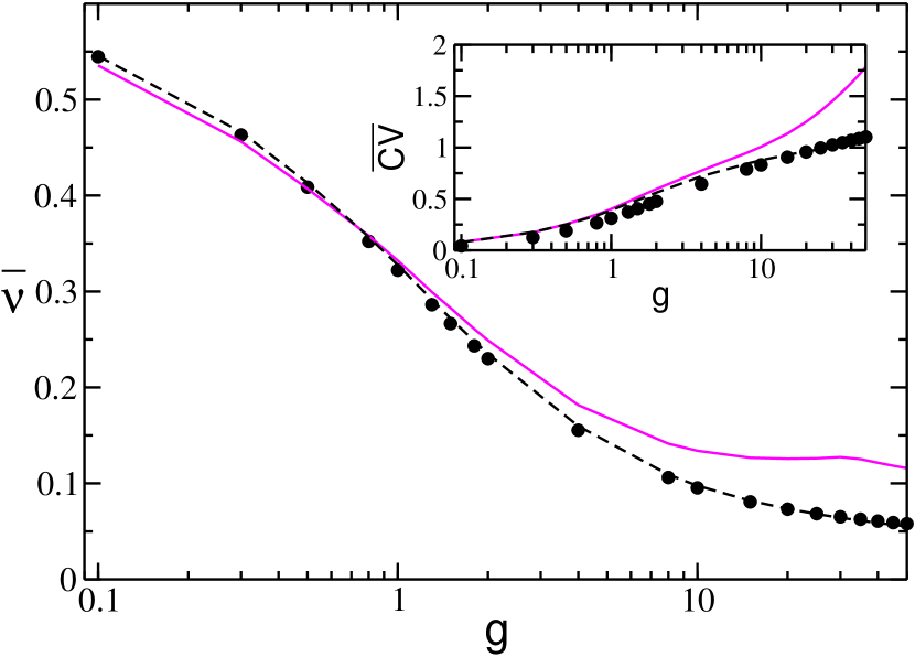
Figure 13: Average network’s frequency $\bar{\nu}$ as a function of the synaptic strength $g$ for instantaneous synapses and uniform distributions $P(I)$ with support $[l_{1},l_{2}]=[1.0,1.5]$. Inset: average coefficient of variation $\overline{CV}$ versus $g$. Filled symbols refer to numerical simulation for $N=400$ and $K=20$, dashed lines to the corresponding analytic solutions reported in Appendices B and C and the solid (magenta) lines to the diffusion approximation. The data have been averaged over a time interval $t_{S}=1\times 10^{6}$ after discarding a transient of $10^{6}$ spikes.

APPENDIX C: Coefficient of variation
for instantaneous synapses

In order to derive the coefficient of variation for the shot noise case it is necessary to obtain the first two moments of the first-passage-time density $q(t)$. By following the same approach as in Appendix B, the time-dependent continuity equation with initial condition $P(v,0)=v_{r}$ is written as

$$\frac{\partial P}{\partial t}+\frac{\partial J}{\partial v}=\rho(t)[\delta(v-v_{r})-\delta(v-\theta)]+\delta(t)\delta(v-v_{r})\;.$$ (33)

As suggested in richardson2010firing , Eq. (33) can be solved by performing a Fourier transform in time and a bilateral Laplace transform in membrane potential. This allows to obtain the Fourier transform of the spike-triggered rate, namely

$$\hat{\rho}(\omega)=\frac{\displaystyle\int_{0}^{\infty}ds\enskip s^{\mathrm{i}\omega}A^{\prime}(s)}{\displaystyle\int_{0}^{\infty}ds\enskip s^{\mathrm{i}\omega}\left[B^{\prime}(s)-A^{\prime}(s)\right]}\quad;$$ (34)

where $A(s)={\rm e}^{sv_{r}}/\tilde{Z}_{0}(s)$ and $B(s)={\rm e}^{s\theta}/\tilde{Z}_{0}(s)$. The Fourier transform of the first-passage-time density is $\hat{q}(\omega)=\frac{\hat{\rho}(\omega)}{1+\hat{\rho}(\omega)}$ and the first and second moment of the distribution are given by

$$\frac{\partial\hat{q}}{\partial\omega}|_{\omega=0}=-\mathrm{i}\langle t\rangle$$ (35)

$$\frac{\partial^{2}\hat{q}}{\partial\omega^{2}}|_{\omega=0}=-\langle t^{2}\rangle$$ (36)

The integrals appearing in Eq. (34) cannot be exactly solved, therefore we have expanded it to the second order obtaining

$$\hat{\rho}(\omega)\simeq\frac{n_{0}+n_{1}\omega+n_{2}\omega^{2}}{d_{0}+d_{1}\omega+d_{2}\omega^{2}}\quad;$$ (37)

where $n_{0}=-1$, $d_{0}=0$, $d_{1}=-\mathrm{i}n_{0}/\nu_{0}$ and

$$n_{1} = \mathrm{i}\int_{0}^{\infty}\log sA^{\prime}(s)ds$$ (38)

$$d_{2} = \int_{0}^{\infty}\frac{\log s}{s}[B(s)-A(s)]ds\qquad.$$ (39)

From the expression (34) we can finally obtain the first and second moment of $q(t)$, namely

$$\langle t\rangle=\frac{1}{\nu_{0}}\quad,\quad\langle t^{2}\rangle=2[d_{1}^{2}+d_{2}+d_{1}n_{1}]\quad.$$ (40)

Once these quantities are known the coefficient of variation can be easily estimated for each neuron with excitability $I$.

The results obtained for the average coefficient of variation $\overline{CV}$ for a sparse network are compared with numerical data and with the diffusion approximation in the inset of Fig. 13. It is evident that the approximation here derived is definitely more accurate than the diffusion approximation for synaptic strengths larger than $g\simeq 1$.

APPENDIX D: Average Firing Rate
for Slow Synapses

In Section V we have examined the average activity of the network for non instantaneous IPSPs with $\alpha$-function profiles. In presence of synaptic filtering, whenever the synaptic time constant is larger than the membrane time constant one can apply the so-called adiabatic approach to derive the firing rate $\nu_{0}$ of a single neuron, as described in  moreno2004 ; moreno2010response .

In this approximation, the output firing rate $\nu_{0}$ of the single neuron driven by a slowly varying stochastic input current $z$ with an arbitrary distribution $P(z)$ is given by

$$\nu_{0}\simeq\int dzP(z)\nu(z)$$ (41)

where $\nu(z)$ is the input to rate transfer function of the neuron under a stationary input which for the LIF neuron is simply:

$$\nu(z)=\left[\ln\left(\frac{z-v_{r}}{z-\theta}\right)\right]^{-1}\quad.$$ (42)

The synaptic filtering induces temporal correlations in the input current $z$, which can be written as:

$$\langle(z(t)-{\mu})(z(t^{\prime})-{\mu})\rangle=\frac{\sigma^{2}}{2\tau_{s}}\exp\left[-\frac{|t-t^{\prime}|}{\tau_{s}}\right]\quad;$$ (43)

here $\tau_{s}$ is the synaptic correlation time. In the case of $\alpha$-pulses, where the rise and decay synaptic times coincide, we can assume that the correlation time is given by $\tau_{s}=\tau_{P}=2\tau_{\alpha}$.

Analogously to the diffusion approximation Ricciardi1971 ; BrunelHakim1999 ; Brunel2000Sparse , the input currents are approximated as a Gaussian noise with mean $\mu$ and variance $\sigma_{z}^{2}=\sigma/2\tau_{s}$. In our network model, a single neuron receives an average current $\mu$ given by Eq. (4) with a standard deviation $\sigma$ given by Eq. (10). In particular, the fraction of active neurons $n_{A}$ entering in the expressions of $\mu$ and $\sigma$ is in this case obtained by the numerical simulations.

Therefore, the single neuron output firing rate reads as

$$\nu_{0}(I) = \int\frac{dz}{\sqrt{2\pi}\sigma_{z}}{\rm e}^{-\frac{(z-\mu(I))^{2}}{2\sigma_{z}^{2}}}\left[\ln\left(\frac{z-v_{r}}{z-\theta}\right)\right]^{-1}\;;$$ (44)

where $I$ is the neuronal excitability.

The average firing rate of the LIF neurons in the network, characterized by an excitability distribution $P(I)$, can be estimated as

$$\bar{\nu}=\int_{\{I_{A}\}}dIP(I)\int_{\theta}\frac{dz}{\sqrt{2\pi}\sigma_{z}}{\rm e}^{-\frac{(z-\mu(I))^{2}}{2\sigma_{z}^{2}}}\left[\ln\left(\frac{z-v_{r}}{z-\theta}\right)\right]^{-1}$$ (45)

where we impose the self-consistent condition that the average output frequency is equal to the average input one.

References

- (1) D Angulo-Garcia, Joshua D. Berke, and A Torcini. Cell assembly dynamics of sparsely-connected inhibitory networks: a simple model for the collective activity of striatal projection neurons. PLoS Comput Biol, 12(2):e1004778, 2015.
- (2) D Angulo-Garcia and A Torcini. Stochastic mean-field formulation of the dynamics of diluted neural networks. Physical Review E, 91(2):022928, 2015.
- (3) David Angulo-Garcia and Alessandro Torcini. Stable chaos in fluctuation driven neural circuits. Chaos, Solitons & Fractals, 69(0):233 – 245, 2014.
- (4) Giancarlo Benettin, Luigi Galgani, Antonio Giorgilli, and Jean-Marie Strelcyn. Lyapunov characteristic exponents for smooth dynamical systems and for hamiltonian systems; a method for computing all of them. part 1: Theory. Meccanica, 15(1):9–20, 1980.
- (5) Joshua D Berke, Murat Okatan, Jennifer Skurski, and Howard B Eichenbaum. Oscillatory entrainment of striatal neurons in freely moving rats. Neuron, 43(6):883–896, 2004.
- (6) Paul C Bressloff and Stephen Coombes. Dynamics of strongly coupled spiking neurons. Neural computation, 12(1):91–129, 2000.
- (7) PC Bressloff and S Coombes. A dynamical theory of spike train transitions in networks of integrate-and-fire oscillators. SIAM Journal on Applied Mathematics, 60(3):820–841, 2000.
- (8) Nicolas Brunel. Dynamics of sparsely connected networks of excitatory and inhibitory spiking neurons. J. Comput. Neurosci., 8(3):183–208, 2000.
- (9) Nicolas Brunel and Vincent Hakim. Fast global oscillations in networks of integrate-and-fire neurons with low firing rates. Neural. Comput., 11(1):1621–1671, mar 1999.
- (10) Ed Bullmore and Olaf Sporns. Complex brain networks: graph theoretical analysis of structural and functional systems. Nature Reviews Neuroscience, 10(3):186–198, 2009.
- (11) Anthony N Burkitt. A review of the integrate-and-fire neuron model: I. homogeneous synaptic input. Biological cybernetics, 95(1):1–19, 2006.
- (12) György Buzsáki and Andreas Draguhn. Neuronal oscillations in cortical networks. Science, 304(5679):1926–1929, 2004.
- (13) Scott Camazine. Self-organization in biological systems. Princeton University Press, 2003.
- (14) RM Capocelli and LM Ricciardi. Diffusion approximation and first passage time problem for a model neuron. Kybernetik, 8(6):214–223, 1971.
- (15) Luis Carrillo-Reid, Fatuel Tecuapetla, Dagoberto Tapia, Arturo Hernández-Cruz, Elvira Galarraga, René Drucker-Colin, and José Bargas. Encoding network states by striatal cell assemblies. Journal of neurophysiology, 99(3):1435–1450, 2008.
- (16) Robert Coultrip, Richard Granger, and Gary Lynch. A cortical model of winner-take-all competition via lateral inhibition. Neural networks, 5(1):47–54, 1992.
- (17) Hiroaki Daido. Onset of cooperative entrainment in limit-cycle oscillators with uniform all-to-all interactions: bifurcation of the order function. Physica D: Nonlinear Phenomena, 91(1):24–66, 1996.
- (18) Paul D Dodson, Joseph T Larvin, James M Duffell, Farid N Garas, Natalie M Doig, Nicoletta Kessaris, Ian C Duguid, Rafal Bogacz, Simon JB Butt, and Peter J Magill. Distinct developmental origins manifest in the specialized encoding of movement by adult neurons of the external globus pallidus. Neuron, 86(2):501–513, 2015.
- (19) Florian Dörfler and Francesco Bullo. Synchronization in complex networks of phase oscillators: A survey. Automatica, 50(6):1539–1564, 2014.
- (20) Bard Ermentrout. Complex dynamics in winner-take-all neural nets with slow inhibition. Neural networks, 5(3):415–431, 1992.
- (21) Tomoki Fukai and Shigeru Tanaka. A simple neural network exhibiting selective activation of neuronal ensembles: from winner-take-all to winners-share-all. Neural computation, 9(1):77–97, 1997.
- (22) Tomoki Fukai and Shigeru Tanaka. A simple neural network exhibiting selective activation of neuronal ensembles: from winner-take-all to winners-share-all. Neural computation, 9(1):77–97, 1997.
- (23) D Golomb, D Hansel, and G Mato. Mechanisms of synchrony of neural activity in large networks. Handbook of biological physics, 4:887–968, 2001.
- (24) David Golomb and John Rinzel. Clustering in globally coupled inhibitory neurons. Physica D: Nonlinear Phenomena, 72(3):259–282, 1994.
- (25) Norberto M Grzywacz and AL Yuille. A model for the estimate of local image velocity by cells in the visual cortex. Proceedings of the Royal Society of London B: Biological Sciences, 239(1295):129–161, 1990.
- (26) Peter Hänggi, Peter Talkner, and Michal Borkovec. Reaction-rate theory: fifty years after kramers. Reviews of modern physics, 62(2):251, 1990.
- (27) Omri Harish and David Hansel. Asynchronous rate chaos in spiking neuronal circuits. PLoS Comput Biol, 11(7):e1004266, 2015.
- (28) Ronald M Harris-Warrick. Dynamic biological networks: the stomatogastric nervous system. MIT press, 1992.
- (29) Laurent Itti and Christof Koch. Computational modelling of visual attention. Nature reviews neuroscience, 2(3):194–203, 2001.
- (30) Sven Jahnke, Raoul-Martin Memmesheimer, and Marc Timme. Stable irregular dynamics in complex neural networks. Phys. Rev. Lett., 100:048102, Jan 2008.
- (31) Sven Jahnke, Raoul-Martin Memmesheimer, and Marc Timme. How chaotic is the balanced state? Front. Comp. Neurosci., 3(13), Nov 2009.
- (32) Jonathan Kadmon and Haim Sompolinsky. Transition to chaos in random neuronal networks. Physical Review X, 5(4):041030, 2015.
- (33) BS Kerner and Vyacheslav Vladimirovich Osipov. Self-organization in active distributed media: scenarios for the spontaneous formation and evolution of dissipative structures. Physics-Uspekhi, 33(9):679–719, 1990.
- (34) MA Komarov, GV Osipov, and JAK Suykens. Sequentially activated groups in neural networks. EPL (Europhysics Letters), 86(6):60006, 2009.
- (35) Tibor Koos, James M Tepper, and Charles J Wilson. Comparison of ipscs evoked by spiny and fast-spiking neurons in the neostriatum. The Journal of neuroscience, 24(36):7916–7922, 2004.
- (36) Yoshiki Kuramoto. Chemical oscillations, waves, and turbulence, volume 19. Springer Science & Business Media, 2012.
- (37) José L Lanciego, Natasha Luquin, and José A Obeso. Functional neuroanatomy of the basal ganglia. Cold Spring Harbor perspectives in medicine, 2(12):a009621, 2012.
- (38) Daniel B Larremore, Woodrow L Shew, Edward Ott, Francesco Sorrentino, and Juan G Restrepo. Inhibition causes ceaseless dynamics in networks of excitable nodes. Physical review letters, 112(13):138103, 2014.
- (39) Simon B Laughlin and Terrence J Sejnowski. Communication in neuronal networks. Science, 301(5641):1870–1874, 2003.
- (40) Gilles Laurent. Olfactory network dynamics and the coding of multidimensional signals. Nature Reviews Neuroscience, 3(11):884–895, 2002.
- (41) Stefano Luccioli, Simona Olmi, Antonio Politi, and Alessandro Torcini. Collective dynamics in sparse networks. Phys. Rev. Lett., 109:138103, Sep 2012.
- (42) Stefano Luccioli and Antonio Politi. Irregular Collective Behavior of Heterogeneous Neural Networks. Phys. Rev. Lett., 105(15):158104+, October 2010.
- (43) Nicolas Mallet, Benjamin R Micklem, Pablo Henny, Matthew T Brown, Claire Williams, J Paul Bolam, Kouichi C Nakamura, and Peter J Magill. Dichotomous organization of the external globus pallidus. Neuron, 74(6):1075–1086, 2012.
- (44) Nicolas Mallet, Robert Schmidt, Daniel Leventhal, Fujun Chen, Nada Amer, Thomas Boraud, and Joshua D Berke. Arkypallidal cells send a stop signal to striatum. Neuron, 89(2):308–316, 2016.
- (45) Eve Marder and Dirk Bucher. Central pattern generators and the control of rhythmic movements. Current biology, 11(23):R986–R996, 2001.
- (46) Hans Meinhardt. Models of biological pattern formation, volume 6. Academic Press London, 1982.
- (47) Benjamin R Miller, Adam G Walker, Anand S Shah, Scott J Barton, and George V Rebec. Dysregulated information processing by medium spiny neurons in striatum of freely behaving mouse models of huntington’s disease. Journal of neurophysiology, 100(4):2205–2216, 2008.
- (48) Renato E Mirollo and Steven H Strogatz. Synchronization of pulse-coupled biological oscillators. SIAM Journal on Applied Mathematics, 50(6):1645–1662, 1990.
- (49) Michael Monteforte and Fred Wolf. Dynamic flux tubes form reservoirs of stability in neuronal circuits. Phys. Rev. X, 2:041007, Nov 2012.
- (50) Rubén Moreno-Bote and Néstor Parga. Role of synaptic filtering on the firing response of simple model neurons. Physical review letters, 92(2):028102, 2004.
- (51) Rubén Moreno-Bote and Néstor Parga. Response of integrate-and-fire neurons to noisy inputs filtered by synapses with arbitrary timescales: Firing rate and correlations. Neural Computation, 22(6):1528–1572, 2010.
- (52) Thomas Nowotny and Mikhail I Rabinovich. Dynamical origin of independent spiking and bursting activity in neural microcircuits. Physical review letters, 98(12):128106, 2007.
- (53) S Olmi, A Politi, and A Torcini. Linear stability in networks of pulse-coupled neurons. Front. Comput. Neurosci., 8(8), 2014.
- (54) Simona Olmi, David Angulo-Garcia, Alberto Imparato, and Alessandro Torcini. The influence of synaptic weight distribution on the activity of balanced networks. preprint, 2016.
- (55) Simona Olmi, Roberto Livi, Antonio Politi, and Alessandro Torcini. Collective oscillations in disordered neural networks. Phys. Rev. E, 81(4 Pt 2), April 2010.
- (56) Srdjan Ostojic. Two types of asynchronous activity in networks of excitatory and inhibitory spiking neurons. Nature neuroscience, 17(4):594–600, 2014.
- (57) André Parent and Lili-Naz Hazrati. Functional anatomy of the basal ganglia. i. the cortico-basal ganglia-thalamo-cortical loop. Brain Research Reviews, 20(1):91–127, 1995.
- (58) Arkady Pikovsky and Michael Rosenblum. Dynamics of globally coupled oscillators: Progress and perspectives. Chaos: An Interdisciplinary Journal of Nonlinear Science, 25(9):097616, 2015.
- (59) Henrike Planert, Thomas K Berger, and Gilad Silberberg. Membrane properties of striatal direct and indirect pathway neurons in mouse and rat slices and their modulation by dopamine. PloS one, 8(3):e57054, 2013.
- (60) Dietmar Plenz. When inhibition goes incognito: feedback interaction between spiny projection neurons in striatal function. Trends in neurosciences, 26(8):436–443, 2003.
- (61) Dietmar Plenz and Stephen T Kitai. Up and down states in striatal medium spiny neurons simultaneously recorded with spontaneous activity in fast-spiking interneurons studied in cortex–striatum–substantia nigra organotypic cultures. The Journal of Neuroscience, 18(1):266–283, 1998.
- (62) Antonio Politi and Michael Rosenblum. Equivalence of phase-oscillator and integrate-and-fire models. Physical Review E, 91(4):042916, 2015.
- (63) Antonio Politi and Alessandro Torcini. Stable chaos. In Nonlinear Dynamics and Chaos: Advances and Perspectives, pages 103–129. Springer, 2010.
- (64) Adam Ponzi and Jeff Wickens. Sequentially switching cell assemblies in random inhibitory networks of spiking neurons in the striatum. The Journal of Neuroscience, 30(17):5894–5911, 2010.
- (65) Adam Ponzi and Jeff Wickens. Input dependent cell assembly dynamics in a model of the striatal medium spiny neuron network. Frontiers in systems neuroscience, 6, 2012.
- (66) Adam Ponzi and Jeffery R Wickens. Optimal balance of the striatal medium spiny neuron network. PLoS computational biology, 9(4):e1002954, 2013.
- (67) Mikhail I Rabinovich and Pablo Varona. Robust transient dynamics and brain functions. Frontiers in computational neuroscience, 5:24, 2011.
- (68) Alfonso Renart, Rubén Moreno-Bote, Xiao-Jing Wang, and Néstor Parga. Mean-driven and fluctuation-driven persistent activity in recurrent networks. Neural. Comput., 19(1):1–46, 2007.
- (69) Luigi M Ricciardi. Diffusion processes and related topics in biology, volume 14. Springer Science & Business Media, 2013.
- (70) Magnus JE Richardson and Rupert Swarbrick. Firing-rate response of a neuron receiving excitatory and inhibitory synaptic shot noise. Physical review letters, 105(17):178102, 2010.
- (71) Francisco A Rodrigues, Thomas K DM Peron, Peng Ji, and Jürgen Kurths. The kuramoto model in complex networks. Physics Reports, 610:1–98, 2016.
- (72) Yousheng Shu, Andrea Hasenstaub, and David A McCormick. Turning on and off recurrent balanced cortical activity. Nature, 423(6937):288–293, 2003.
- (73) Peter Somogyi, Gabor Tamas, Rafael Lujan, and Eberhard H Buhl. Salient features of synaptic organisation in the cerebral cortex. Brain research reviews, 26(2):113–135, 1998.
- (74) Steven H Strogatz. Exploring complex networks. Nature, 410(6825):268–276, 2001.
- (75) Lorenzo Tattini, Simona Olmi, and Alessandro Torcini. Coherent periodic activity in excitatory erdös-renyi neural networks: the role of network connectivity. Chaos, 22(2):023133, jun 2012.
- (76) Stefano Taverna, Ema Ilijic, and D James Surmeier. Recurrent collateral connections of striatal medium spiny neurons are disrupted in models of parkinson’s disease. The Journal of neuroscience, 28(21):5504–5512, 2008.
- (77) Stefano Taverna, Yvette C Van Dongen, Henk J Groenewegen, and Cyriel MA Pennartz. Direct physiological evidence for synaptic connectivity between medium-sized spiny neurons in rat nucleus accumbens in situ. Journal of neurophysiology, 91(3):1111–1121, 2004.
- (78) James M Tepper, Tibor Koós, and Charles J Wilson. Gabaergic microcircuits in the neostriatum. Trends in neurosciences, 27(11):662–669, 2004.
- (79) LS Tsimring, NF Rulkov, ML Larsen, and Michael Gabbay. Repulsive synchronization in an array of phase oscillators. Physical review letters, 95(1):014101, 2005.
- (80) Henry C Tuckwell. Introduction to theoretical neurobiology: Volume 2, nonlinear and stochastic theories, volume 8. Cambridge University Press, 2005.
- (81) Mark J Tunstall, Dorothy E Oorschot, Annabel Kean, and Jeffery R Wickens. Inhibitory interactions between spiny projection neurons in the rat striatum. Journal of Neurophysiology, 88(3):1263–1269, 2002.
- (82) Ekkehard Ullner and Antonio Politi. Self-sustained irregular activity in an ensemble of neural oscillators. Physical Review X, 6(1):011015, 2016.
- (83) Carl van Vreeswijk. Partial synchronization in populations of pulse-coupled oscillators. Phys. Rev. E, 54(5):5522–5537, November 1996.
- (84) Vladimir K Vanag, Lingfa Yang, Milos Dolnik, Anatol M Zhabotinsky, and Irving R Epstein. Oscillatory cluster patterns in a homogeneous chemical system with global feedback. Nature, 406(6794):389–391, 2000.
- (85) Xiao-Jing Wang and György Buzsáki. Gamma oscillation by synaptic inhibition in a hippocampal interneuronal network model. The journal of Neuroscience, 16(20):6402–6413, 1996.
- (86) Arthur T Winfree. The geometry of biological time, volume 12. Springer Science & Business Media, 2001.
- (87) Yuan Xiong, Chuan-Hsiang Huang, Pablo A Iglesias, and Peter N Devreotes. Cells navigate with a local-excitation, global-inhibition-biased excitable network. Proceedings of the National Academy of Sciences, 107(40):17079–17086, 2010.
- (88) Alan L Yuille and Norberto M Grzywacz. A winner-take-all mechanism based on presynaptic inhibition feedback. Neural Computation, 1(3):334–347, 1989.
- (89) Rüdiger Zillmer, Nicolas Brunel, and David Hansel. Very long transients, irregular firing, and chaotic dynamics in networks of randomly connected inhibitory integrate-and-fire neurons. Phys. Rev. E, 79:031909, Mar 2009.
- (90) Rüdiger Zillmer, Roberto Livi, Antonio Politi, and Alessandro Torcini. Desynchronization in diluted neural networks. Phys. Rev. E, 74(3):036203, 2006.
- (91) Rüdiger Zillmer, Roberto Livi, Antonio Politi, and Alessandro Torcini. Stability of the splay state in pulse-coupled networks. Phys. Rev. E, 76:046102, Oct 2007.