Recovering lost 21 cm radial modes via cosmic tidal reconstruction

Abstract

21 cm intensity mapping has emerged as a promising technique to map the large-scale structure of the Universe, at redshifts $z$ from 1 to 10. Unfortunately, many of the key cross-correlations with the cosmic microwave background and photo-$z$ galaxies have been thought to be impossible due to the foreground contamination for radial modes with small wave numbers. In this paper, we apply tidal reconstruction to the simulated 21 cm fields and recover the lost large-scale radial modes successfully. We estimate the detectability of the cross-correlation signals and find they can be detected at high significance with current 21 cm experiments. The tidal field reconstruction method opens up a new set of possibilities to probe the Universe and is extremely valuable not only for 21 cm surveys but also for cosmic microwave background and photometric-redshift observations.

I Introduction

The current and future cosmic surveys aim to map a large fraction of the Universe with unprecedented precision by observing the large-scale structure (e.g., SDSS Alam et al. (2017), DES Dark Energy Survey Collaboration et al. (2016), PFS Takada et al. (2014), DESI DESI Collaboration et al. (2016), LSST LSST Science Collaboration et al. (2009), Euclid Amendola et al. (2013)) and the cosmic microwave background (CMB) (e.g., Planck Planck Collaboration et al. (2016a), SPT-3G Benson et al. (2014), Advanced ACTPol Henderson et al. (2016), CMB-S4 Abazajian et al. (2016)). Precision measurement of cosmological parameters from the autocorrelations of large-scale structure and CMB observations and the cross-correlations between different observations can improve constraints on the properties of dark energy, modifications to general relativity, neutrino masses, and primordial non-Gaussianities substantially. In addition to these observation methods, 21 cm intensity mapping has emerged as a powerful method to map the large-scale structure of the Universe Chang et al. (2008); Loeb and Wyithe (2008); Seo et al. (2010). Instead of resolving millions of individual galaxies, the 21 cm intensity mapping technique measures the large-scale structure by detecting the aggregate 21 cm emission of neutral hydrogen from many galaxies in large voxels. The redshifted 21 cm emission line which provides the redshift information can be resolved exquisitely in the frequency domain. Therefore, this allows radio telescopes to conduct rapid and efficient surveys of large volumes of the Universe. The ongoing and upcoming 21 cm surveys including CHIME Bandura et al. (2014), HIRAX Newburgh et al. (2016), Tianlai Xu et al. (2015), BINGO Battye et al. (2013), FAST Bigot-Sazy et al. (2016), MeerKAT Santos et al. (2017), and SKA Santos et al. (2015) can improve the baryon acoustic oscillations (BAO) measurements by observing a larger cosmic volume at higher redshifts compared to current galaxy surveys.

The primary challenge for 21 cm intensity mapping experiments is the presence of the astrophysical foregrounds from galactic and extra-galactic synchrotron emissions, which are three orders of magnitude brighter than the cosmological 21 cm signals. The synchrotron foregrounds are known to be spectrally smooth in the frequency domain where the redshifted 21 cm signals from different redshifts fluctuate at different frequencies. In principle, the foregrounds only impact the long wavelength density fluctuations along the line of sight, i.e., the modes with small $k_{\parallel}$ in Fourier space Oh and Mack (2003); Furlanetto et al. (2006). However, the instrumental effects (e.g. spectral response, calibration, etc) further lead to an unsmooth foreground component, often referred as the foreground wedge at the low $k_{\parallel}$ and high $k_{\perp}$ area in Fourier space Datta et al. (2010); Morales et al. (2012); Vedantham et al. (2012); Pober et al. (2013); Pober (2015). The synchrotron foregrounds can be cleaned by exploiting their smooth spectral structure Liu and Tegmark (2011, 2012); Shaw et al. (2014, 2015). As demonstrated in Ref. Shaw et al. (2015), the foregrounds can be cleaned well below the foreground wedge with the precise calibration of the instrument, leaving only $k_{\parallel}<0.02\ h\mathrm{Mpc}^{-1}$ modes unaccessible.

However, while there are not many Fourier modes at $k_{\parallel}<0.02\ h\mathrm{Mpc}^{-1}$, many other cosmological observations such as weak lensing, photometric-redshift galaxies, and integrated Sachs-Wolf (ISW) effect can only probe these modes, i.e., the angular density fluctuations. These observations involve a broad window function along the line of sight and measure the projected modes, i.e., the modes with small $k_{\parallel}$, which are all contaminated by the foreground emissions in 21 cm intensity mapping observations. Therefore, the proposed cross-correlation of 21 cm intensity mapping with weak gravitational lensing Kirk et al. (2015); Pourtsidou et al. (2016); Pourtsidou (2016), photo-$z$ galaxies Kirk et al. (2015); Alonso and Ferreira (2015); Fonseca et al. (2015, 2017); Pourtsidou et al. (2017); Alonso et al. (2017), and ISW effect Pourtsidou et al. (2017) would be severely degraded in the presence of foregrounds. Recovering the lost large-scale radial modes for cross-correlations is thus crucial in order to fully exploit the 21 cm intensity mapping experiments. The cross-correlation measurements will benefit other observations as well, since the cross-correlations are expected to be more robust to the systematics than autocorrelations from individual experiments. It also enables the use of sample variance cancellation technique Seljak (2009) to measure cosmological parameters Alonso and Ferreira (2015); Fonseca et al. (2015, 2017).

Recently a new method called cosmic tidal reconstruction has been developed Pen et al. (2012); Zhu et al. (2016a). The small-scale density fluctuations are significantly affected by the large-scale density field as a consequence of gravitational mode coupling. The large-scale tidal shear field causes anisotropic distortions of the locally measured small-scale matter power spectrum. Such local anisotropic tidal distortions can be exploited to reconstruct the large-scale tidal shear and hence density fields. The reconstruction of gravitational tidal fields from local small-scale matter power spectrum is described by the same formulation as the reconstruction of gravitational lensing induced shear. As shown in Ref. Zhu et al. (2016a), the density modes with small $k_{\parallel}$ and large $k_{\perp}$ are well reconstructed, with cross-correlation coefficient close to $1$ for reconstruction with the full dark matter density field. These reconstructed density modes are exactly those lost in the foreground subtraction of 21 cm experiments. The tidal reconstruction technique enables the reconstruction of lost 21 cm radial modes, which provides important radial information essential for cross-correlating with the CMB and photometric observations.

In this paper, we apply cosmic tidal reconstruction to the simulated 21 cm field with low $k_{\parallel}$ foreground modes subtracted. The small $k_{\parallel}$ radial modes are recovered successfully after tidal reconstruction. Then we cross-correlate the reconstructed 21 cm field with the simulated CMB lensing, photo-$z$ galaxy and ISW effect fields and estimate the detectability of the cross-correlation signals with the current 21 cm experiments. The tidal field reconstruction method provides us a new way to study the large-scale matter distribution in the Universe through cross-correlations and has profound implications for the current and future 21 cm experiments.

The paper is organized as follows. In Sec. II, we introduce the cosmic tidal reconstruction. In Sec. III, we apply tidal field reconstruction to the simulated foreground subtracted 21 cm density field and shows the reconstruction results. Section IV shows the cross-correlation signal recovered after reconstruction and estimates the detectability with current 21 cm experiments. We discuss further improvements and future applications in Sec. V.

II Cosmic tidal reconstruction

The large-scale density field can be reconstructed accurately from the anisotropic tidal distortions of the locally measured matter power spectrum Pen et al. (2012); Zhu et al. (2016a). The basic idea of purely transverse tidal reconstruction has been proposed in Ref. Pen et al. (2012) and further expanded in Ref. Zhu et al. (2016a). In this section, we briefly discuss the physical idea and outline the operational procedure of the tidal field reconstruction. More details of this reconstruction method are presented in Ref. Zhu et al. (2016a).

II.1 Cosmic tides

The evolution of small-scale density perturbations is modulated by long wavelength perturbations during nonlinear structure formation. The gravitational coupling of a long wavelength tidal field with small-scale density fluctuations has been studied extensively Schmidt et al. (2014). The leading-order observable of a long wavelength density perturbation on small-scale density perturbations is described by the large-scale tidal field,

$$t_{ij}=\Phi_{L,ij}-\delta_{ij}\Phi_{L,kk}/3,$$ (1)

where $\Phi_{L}$ is the long wavelength gravitational potential sourced by the long wavelength density perturbation $\delta_{L}$. Here $\Phi_{L,ij}$ denotes partial derivatives of $\Phi_{L}$ to $x^{i}$ and $x^{j}$. Note that we have projected out the trace of $\Phi_{L,ij}$, which corresponds to the local mean density. Since the change of shape is more robust than the change of number density, we shall focus on the gravitational tidal shear, i.e., the traceless tidal field. The locally observed matter power spectrum in the presence of the large-scale tidal field $t_{ij}$ can be calculated using Lagrangian perturbation theory and is given by

$$P(\bm{k},\tau)|_{t_{ij}}=P(k,\tau)+\hat{k}^{i}\hat{k}^{j}t^{(0)}_{ij}P(k,\tau)f(k,\tau),$$ (2)

where $\tau$ is the conformal time, $P(k,\tau)$ is the isotropic linear power spectrum, $\hat{\bm{k}}$ is the unit vector, the superscript $(0)$ denotes the initial time defined in perturbation calculation. The coupling of the large-scale tidal field to small-scale density fluctuations is described by the tidal coupling coefficient

$$f(k,\tau)=2\alpha(\tau)-\beta(\tau)\frac{d\>\mathrm{ln}\>P(k,\tau)}{d\>\mathrm{ln}\>k},$$ (3)

where $\alpha(\tau)$ and $\beta(\tau)$ are integrals involving background cosmological parameters and can be computed numerically Schmidt et al. (2014); Zhu et al. (2016a). The above result only includes the leading order effect of the coupling between the large-scale tidal field and small-scale density fluctuations. In reality the density field is quite nonlinear and involves all higher order interactions. The reconstructed density field would be biased when the theoretical description of the nonlinear coupling in the above equation is not accurate. This problem can be addressed using the transfer function calibrated from simulations Zhu et al. (2016a).

The traceless tidal tensor $t_{ij}$ can be decomposed into five independently observable components ($\gamma_{1}$, $\gamma_{2}$, $\gamma_{x}$, $\gamma_{y}$, $\gamma_{z}$) Zhu et al. (2016a). We notice that the two transverse shear terms,

$$\gamma_{1}=(\Phi_{L,11}-\Phi_{L,22})/2,\ \gamma_{2}=\Phi_{L,12},$$ (4)

which describe quadrupolar distortions in the tangential plane perpendicular to the line of sight, are less affected by peculiar velocities. Thus, in the following computation we shall use them to perform reconstruction. Once we have the tidal shear terms $\gamma_{1}$ and $\gamma_{2}$, the reconstructed density field can be obtained by

$$\delta_{r}(\bm{k})=\frac{Ak^{2}}{(k_{1}^{2}+k_{2}^{2})^{2}}\bigg{[}(k_{1}^{2}-k_{2}^{2})\gamma_{1}(\bm{k})+2k_{1}k_{2}\gamma_{2}(\bm{k})\bigg{]},$$ (5)

where $A$ is the normalization coefficient. Since we only use two transverse tidal shear fields $\gamma_{1}$ and $\gamma_{2}$ for reconstruction, the change of the large-scale density field along the line of sight is inferred from the variations of $\gamma_{1}$ and $\gamma_{2}$ along the $z$ axis. The noise for the reconstructed density field is anisotropic in Fourier space. The tidal reconstruction technique works best for modes in the high $k_{\perp}$ and low $k_{\parallel}$ region, which cannot be obtained from 21 cm surveys directly but contribute substantially to observables from other cosmological observations as discussed above. Cosmic tidal reconstruction provides a new possible way to recover the lost radial modes and to improve the cross-correlation signals.

II.2 Reconstruction algorithm

In this subsection, we describe the tidal reconstruction method used in the next section.

II.2.1 Reducing nonlinearities

The first step is to smooth the nonlinear density field with a Gaussian kernel,

$$\delta_{R}(\bm{k})=W_{R}(\bm{k})\delta(\bm{k}),$$ (6)

where

$$W_{R}(\bm{k})=\mathrm{exp}(-k^{2}R^{2}/2),$$ (7)

which filters out small-scale structures. The perturbative description of tidal coupling in Eq. (2) is not valid in the strong non-Gaussian regions. We need to smooth small-scale nonlinear structures to reduce nonlinearities. Here, we take $R=1.25\ \mathrm{Mpc}/h$, which is close to the optimal filter scale as demonstrated in Refs. Pen et al. (2012); Zhu et al. (2016a).

The second step is to Gaussianize the smoothed density field by taking a logarithmic transform or mapping the density fluctuations into a Gaussian distribution according to their density values. We shall use the latter method since the tidal shear estimator we use is derived under the Gaussian assumption. Otherwise we can only use the limited number of density modes on large scales where the Gaussian assumption is valid, but the reconstruction will be degraded significantly.

II.2.2 Estimating tidal shear fields

The coupling of the large-scale tidal field and small-scale density fluctuations leads to a local anisotropy of quadratic statistics. The tidal shear fields can be reconstructed by applying quadratic estimators to the Gaussianized density field $\delta_{g}$ as

$$\hat{\gamma}_{1}(\bm{x})=\big{[}\delta_{g}^{w_{1}}(\bm{x})\delta_{g}^{w_{1}}(\bm{x})+\delta_{g}^{w_{2}}(\bm{x})\delta_{g}^{w_{2}}(\bm{x})\big{]}/2,$$

$$\hat{\gamma}_{2}(\bm{x})=\big{[}\delta_{g}^{w_{1}}(\bm{x})\delta_{g}^{w_{2}}(\bm{x})\big{]},$$ (8)

where

$$\delta_{g}^{w_{1}}(\bm{k})=i\hat{k}_{1}w(\bm{k})\delta_{g}(\bm{k}),\ \delta_{g}^{w_{2}}(\bm{k})=i\hat{k}_{2}w(\bm{k})\delta_{g}(\bm{k}),$$ (9)

and the filter is

$$w(\bm{k})=\frac{\sqrt{P(\bm{k})f(\bm{k})}}{P_{\mathrm{tot}}(\bm{k})},$$ (10)

Here, $P_{\mathrm{tot}}(\bm{k})$ is the total power spectrum of the 21 cm density field which includes both the signal and noise. We find that the reconstruction performance is not sensitive to the exact shape of the filter. The reconstruction of tidal shear fields is similar to the reconstruction of lensing shear fields from 21 cm temperature fields. The quadratic estimators presented above can be constructed using either the maximum likelihood method or the inverse variance weighting Lu and Pen (2008); Lu et al. (2010); Bucher et al. (2012).

II.2.3 Generating the density field

After we get the tidal shear fields $\gamma_{1}$ and $\gamma_{2}$, the tidal reconstructed density field is given by Eq. (5). In general, the reconstructed field $\delta_{r}(\bm{k})$ can be written as

$$\delta_{r}(\bm{k})=C(\bm{k})\delta(\bm{k})+N(\bm{k}),$$ (11)

where $C(\bm{k})=P_{\delta_{r}\delta}(\bm{k})/P_{\delta}(\bm{k})$, $\delta(\bm{k})$ is the original matter density field and $N(\bm{k})$ includes the noises from 21 cm observation and from reconstruction. The factor $C(\bm{k})$, often referred as the propagator, quantifies how much information of the original density distribution is reconstructed. To get an unbiased measurement of the original density field, we can deconvolve the propagator $C(\bm{k})$ from the reconstructed field,

$$\hat{\delta}_{r}=\delta_{r}(\bm{k})/C(\bm{k})=\delta(\bm{k})+N(\bm{k})/C(\bm{k}).$$ (12)

This factor can be computed by performing reconstruction with the simulated observation mock data Zhu et al. (2018); Seljak et al. (2017); Schmittfull et al. (2017). As we deconvolve the propagator, the reconstructed density field is unbiased. The cross-correlation coefficient quantifies the reconstruction noise.

III Implementation and results

To test the performance of reconstruction, we run an ensemble of six $N$-body simulations with the ${\tt CUBEP^{3}M}$ code Harnois-Déraps et al. (2013). Each simulation involves $1024^{3}$ dark matter particles in a cubic box of side length $1200\ \mathrm{Mpc}/h$. We use the snapshot at redshift $z=1$ and generate the dark matter density field on a $1024^{3}$ grid. We could approximately use the dark matter density to represent the 21 cm source distribution, i.e., the neutral hydrogen. This is a good approximation since the neutral hydrogen traces the total mass distribution fairly well at low redshifts (see Refs. Castorina and Villaescusa-Navarro (2017); White and Padmanabhan (2017) for more discussions about the modeling of neutral hydrogen in the Universe). However, the realistic neutral hydrogen density field should also include the fluctuation of neutral hydrogen fraction in the Universe, the redshift space distortion effect due to the peculiar velocity, etc. We plan to study these in future.

There are several noises for 21 cm experiments we need to consider to model the observed 21 cm signal from intensity mapping observations, including the astrophysical foreground, the receiver noise, and the shortest baseline for inteferometers.

A detailed 21 cm foreground subtraction simulation is beyond the scope of this paper. Instead we simply use a high-pass filter along the line of sight,

$$W_{\mathrm{fs}}(k_{\parallel})=1-e^{-k_{\parallel}^{2}R_{\mathrm{fs}}^{2}/2},$$ (13)

which removes the small $k_{\parallel}$ density modes, to simulate the loss of modes due to foreground contamination. We use the two different foreground scales $R_{\mathrm{fs}}=60\ \mathrm{Mpc}/h$ and $15\ \mathrm{Mpc}/h$ in reconstruction, which give $W_{\mathrm{fs}}=0.5$ at $k_{\parallel}=0.02\ h\mathrm{Mpc}^{-1}$ and $0.08\ h\mathrm{Mpc}^{-1}$, respectively. The former is an optimal case, i.e., we only lose modes with $k_{\parallel}\lesssim 0.02\ h\mathrm{Mpc}^{-1}$ Shaw et al. (2015), while the latter is already achieved in the current 21 cm observations Masui et al. (2013); Switzer et al. (2013).

For 21 cm observations around redshift $z=1$, the resolution of small-scale structures is mainly determined by the thermal noise. The thermal noise power $P_{N}$ is about $150-600\ (\mathrm{Mpc}/h)^{3}$ for a HIRAX-like interferometer, depending on the neutral hydrogen fraction and bias White and Padmanabhan (2017). We assume the experimental noise to be zero above a cut off scale and infinity below this scale. We choose it to be $k_{N}=0.6\ h\mathrm{Mpc}^{-1}$, which is about the scale where the thermal noise power dominates over the matter power spectrum. The effect of the experimental noise can be modeled by applying a step function

$$\Theta(k_{N}-k)=\left\{\begin{array}[]{ll}1,&k\leq k_{N}\\ 0,&k>k_{N}\end{array}\right.,$$

to the dark matter density field from the simulation.

Most current 21 cm intensity mapping experiments are carried on interferometers. The largest angular scale that can be probed is decided by the shortest baseline of the interferometer. We also use a step function

$$\Theta(\ell-\ell_{s})=\left\{\begin{array}[]{ll}1,&\ell\geq\ell_{s}\\ 0,&\ell<\ell_{s}\end{array}\right.,$$

to model this effect, where the largest scale can be probed is $\ell_{s}=115$ or $k_{\perp}=0.05\ h/\mathrm{Mpc}$ at redshift $z=1$. This corresponds to a shortest baseline of $\sim 7\ \mathrm{m}$.

In summary, the simulated 21 cm field from intensity mapping is given by

$$\delta_{\mathrm{IM}}(\bm{k})=\delta(\bm{k})W_{\mathrm{fs}}(k_{\parallel})\Theta(k_{N}-k)\Theta(\ell-\ell_{s}),$$ (14)

where $\delta(\bm{k})$ is the full density field from the simulation. Note that $\ell$ is the angular wave number, defined as $\ell+1/2=k_{\perp}\chi(z)$. We apply tidal reconstruction to the simulated 21 cm field and get the reconstructed density field defined in Eq. (12) using the algorithm described above.

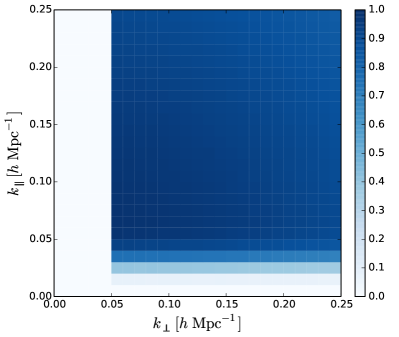
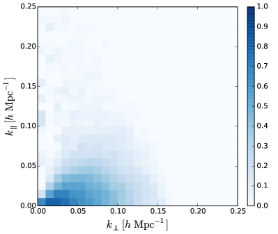
Figure 1: Top: The cross-correlation coefficient of the simulated 21 cm intensity mapping field $\delta_{\mathrm{IM}}(\bm{k})$ with the original full dark matter density field $\delta(\bm{k})$. Bottom: The cross-correlation coefficient of the reconstructed density field $\hat{\delta}_{r}(\bm{k})$ with the original full dark matter density field $\delta(\bm{k})$. These results are for the foreground scale $R_{\mathrm{fs}}=60\ \mathrm{Mpc}/h$, where modes with $k_{\parallel}\lesssim 0.02\ h\mathrm{Mpc}^{-1}$ are subtracted.

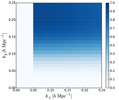
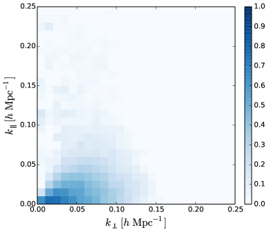
Figure 2: Same as Fig. 1, but for the foreground scale $R_{\mathrm{fs}}=15\ \mathrm{Mpc}/h$, where modes with $k_{\parallel}\lesssim 0.08\ h\mathrm{Mpc}^{-1}$ are subtracted.

Figure 1 shows the two-dimensional cross-correlation coefficient of the 21 cm intensity mapping field with the full dark matter density field. We also plot the cross-correlation coefficient of the reconstructed density field with the full dark matter density field. These results are for the foreground scale $R_{\mathrm{fs}}=60\ \mathrm{Mpc}/h$, i.e., $k_{\parallel}=0.02\ h\mathrm{Mpc}^{-1}$. The lost large-scale radial modes are successfully recovered by tidal reconstruction. Figure 2 shows the corresponding results for the foreground scale $R_{\mathrm{fs}}=15\ \mathrm{Mpc}/h$, i.e., $k_{\parallel}=0.08\ h\mathrm{Mpc}^{-1}$. We note that the loss of more large-scale radial modes does not degrade the performance of reconstruction significantly. This is because the tidal reconstruction method uses small-scale structure to reconstruct the large-scale density field and the reconstruction performance mainly depends on the number of small-scale modes.

To clearly see how well the $k_{\parallel}\sim 0$ modes relevant for cross-correlations are reconstructed, we compute the projected density field by averaging the three-dimensional density field along the line of sight, i.e., the $z$ axis of the simulation box. Figure 3 shows the cross-correlation coefficients of the projected full dark matter density field with the projected reconstructed density fields for the foreground scales $k_{\parallel}=0.02\ h\mathrm{Mpc}^{-1}$ and $0.08\ h\mathrm{Mpc}^{-1}$. The angular scale $\ell$ is related to the three-dimensional wave number $k$ through $\ell+1/2=k\chi(z=1)$, where $\chi(z=1)=2301\ \mathrm{Mpc}/h$ is the comoving distance to redshift $z=1$ Loverde and Afshordi (2008). The cross-correlation coefficient is larger than $0.7$ at scale $\ell\lesssim 100$ for the small $k_{\parallel}$ foreground and larger than $0.65$ at scale $\ell\lesssim 100$ for the large $k_{\parallel}$ foreground. Therefore, the successful reconstruction of $k_{\parallel}\sim 0$ modes makes the cross correlation of 21 cm intensity mapping surveys with the CMB and photometric galaxy surveys possible.

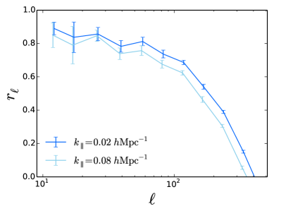
Figure 3: The cross-correlation coefficients of the projected full dark matter density field with the projected reconstructed density fields for the foreground scales $k_{\parallel}=0.02\ h\mathrm{Mpc}^{-1}$ and $0.08\ h\mathrm{Mpc}^{-1}$. The angular scale $\ell$ is related to the three-dimensional wave number $k$ through $\ell+1/2=k\chi(z=1)$, where $\chi(z=1)=2301\ \mathrm{Mpc}/h$ is the comoving distance to redshift $z=1$. The cross-correlation coefficient is larger than $0.7$ and $0.65$ at scale $\ell\lesssim 100$ for the small $k_{\parallel}$ and large $k_{\parallel}$ foreground scales, respectively. The error bars are estimated using the bootstrap resampling method.

IV Cross-correlation signals

To estimate the detectability of the cross-correlation signals, we generate the CMB lensing convergence field, the angular galaxy distribution from photometric-redshift surveys, and the temperature fluctuation due to the ISW effect from the same simulation used for tidal reconstruction. They are line of sight projections of the dark matter density field,

$$\delta_{i}(\bm{\theta})=\int d\chi W_{i}(\chi)\delta(\chi\bm{\theta},\chi),$$ (15)

where $W_{i}(\chi)$ is the window function. The angular cross-correlation power spectrum is then given by

$$C_{\ell}^{ij}=\int d\chi\frac{W_{i}(\chi)W_{j}(\chi)}{\chi^{2}}P_{\delta}\bigg{(}k=\frac{\ell+1/2}{\chi},\chi\bigg{)}.$$ (16)

When $i=j$, this formula gives the power spectrum for $\delta_{i}(\bm{\theta)}$. The error for the cross-correlation signal is

$$\sigma(C_{\ell}^{ij})=\bigg{[}\frac{1}{(2\ell+1)f_{\mathrm{sky}}\Delta\ell}((C_{\ell}^{ij})^{2}+\hat{C}_{\ell}^{i}\hat{C}_{\ell}^{j})\bigg{]}^{1/2},$$ (17)

where $\hat{C}$ includes the signal and the corresponding noise. We set $\ell_{\mathrm{min}}=12$ and choose $f_{\mathrm{sky}}$ to be $0.25$ for CMB lensing and photo-$z$ galaxies, and $1$ for ISW effect. Notice that we use the projection of the reconstructed 21 cm field for cross correlation.

IV.1 CMB lensing

The lensing convergence field from CMB lensing reconstruction is a weighted projection of the dark matter density fluctuations along the line of sight to the last scattering surface,

$$\kappa(\bm{\theta})=\int_{0}^{\chi_{s}}d\chi W_{\kappa}(\chi)\delta(\chi\bm{\theta},\chi),$$ (18)

where the lensing kernel

$$W_{\kappa}(\chi)=\frac{3\Omega_{m0}H_{0}^{2}\chi(\chi_{s}-\chi)}{2a(\chi)\chi_{s}},$$ (19)

and $\chi_{s}=\chi(z_{s}=1090)$. Because the CMB lensing kernel is very broad in redshift, we take its value at redshift $z=1$ in the line of sight projection. The noise for CMB lensing measurement is assumed to be the same as the Planck 2015 results Planck Collaboration et al. (2016b).

Figure 4 shows the theoretical and measured cross power spectra. We also plot the error bars of the cross power spectrum for the $k_{\parallel}=0.02\ h\mathrm{Mpc}^{-1}$ foreground. Since the error bars for the $k_{\parallel}=0.08\ h\mathrm{Mpc}^{-1}$ foreground are just slightly larger, we only plot the error bars for the small $k_{\parallel}$ foreground. The total signal-to-noise ratio is $9.4$ and $8.0$ for the small and large $k_{\parallel}$ foregrounds.

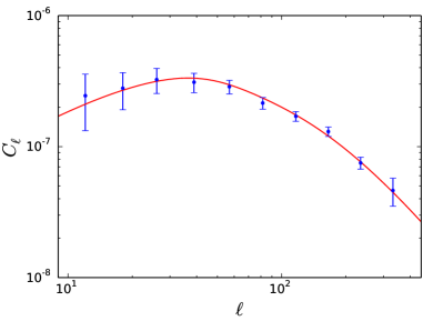
Figure 4: The cross-correlation signal of 21 cm intensity mapping and CMB lensing. The solid line shows the theoretical cross power spectrum and the data points are measured from the simulations. The error bars are for the foreground scale $R_{\mathrm{fs}}=60\ h/\mathrm{Mpc}$, i.e., $k_{\parallel}=0.02\ h\mathrm{Mpc}^{-1}$.

IV.2 Photo-$z$ galaxies

We calculate the projected galaxy density field at $z\sim 1$ with usual photo-$z$ bin width of $0.2$, i.e., $z_{\mathrm{p}}\in(0.9,1.1)$. We adopt the galaxy distribution characterized by

$$n(z)\propto z^{\alpha}\mathrm{exp}\big{[}-(z/z^{*})^{\beta}\big{]},$$ (20)

with $\alpha=2$, $z^{*}=0.5$, $\beta=1$ and assume the photometric-redshift scatter $\mathcal{P}(z_{\mathrm{p}}|z)$ is perfectly known to be in a Gaussian form with photo-$z$ rms error $\sigma_{z}=0.05(1+z)$. The angular galaxy distribution is given by

$$\delta_{g}(\bm{\theta})=\int_{0}^{\infty}dzW_{\mathrm{p}}(z)b(z)\delta(\chi(z)\bm{\theta},\chi(z))\ ,$$ (21)

where the window function

$$W_{\mathrm{p}}(z)\propto n(z)\int_{0.9}^{1.1}\mathcal{P}(z_{\mathrm{p}}|z)dz_{\mathrm{p}}\$$ (22)

with normalization $\int W_{\mathrm{p}}(z)dz=1$. We assume a linear galaxy bias $b(z)=1+0.84z$. For photo-$z$ galaxies from LSST-like surveys, the shot noise is negligible on degree scales.

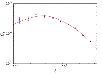
Figure 5: The cross-correlation signal of 21 cm intensity mapping and photo-$z$ galaxies. The solid curve shows the theoretical cross power spectrum and the data points are measured from the simulations. The error bars are for the foreground scale $R_{\mathrm{fs}}=60\ h/\mathrm{Mpc}$, i.e., $k_{\parallel}=0.02\ h\mathrm{Mpc}^{-1}$.

Figure 5 shows the theoretical and measured cross power spectra. We also plot the error bars for the foreground scale $k_{\parallel}=0.02\ h\mathrm{Mpc}^{-1}$. The total signal-to-noise ratio is $24.3$ and $14.4$ for the small and large $k_{\parallel}$ foregrounds, respectively. The significant cross-correlation between reconstructed 21 cm field and photo-$z$ galaxies makes it possible to calibrate the redshift distribution of galaxies from imaging surveys using 21 cm intensity mapping surveys Alonso et al. (2017).

IV.3 ISW effect

The fractional CMB temperature fluctuations induced by the ISW effect is given as

$$\bigg{(}\frac{\Delta T}{T}\bigg{)}_{\mathrm{ISW}}(\bm{\theta})=-2\int_{0}^{\chi_{s}}d\chi\frac{\partial\Phi(\chi\bm{\theta},\chi)}{\partial\chi}\ .$$ (23)

In Fourier space, approximating that the evolution of $\delta(\bm{k},t)$ with time is given by linear theory $\dot{\delta}(\bm{k},t)=\dot{D}(t)\delta(\bm{k},t=0)$, we have

$$\frac{\partial\Phi(\bm{k},\chi)}{\partial\chi}=-\frac{3\Omega_{m0}H_{0}^{2}}{2a(\chi)}\frac{\partial\mathrm{ln}(D/a)}{\partial\chi}\frac{\delta(\bm{k},\chi)}{k^{2}}\ ,$$ (24)

where $D$ is the linear growth function. In our implementation, we approximate the time dependent factor as a constant across the simulation box. For the ISW effect, the noise is just the large-scale CMB power $C_{\ell}^{TT}$.

Figure 6 shows the theoretical and measured cross power spectra. We plot the error bars for the small $k_{\parallel}$ foreground. The total signal-to-noise ratio is $3.1$ and $3.0$ for the small and large $k_{\parallel}$ foregrounds. The redshift information from 21 cm intensity mapping allows us to constrain the expansion history of the Universe as a function of redshift. The detectability of ISW effect can be further improved by including CMB polarization data Liu et al. (2011).

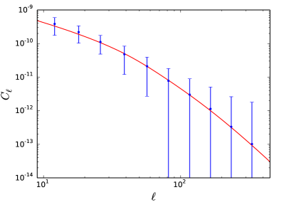
Figure 6: The cross-correlation signal of 21 cm intensity mapping and ISW effect. The solid curve shows the theoretical signal and the data points are measured from the simulations. The error bars are for the foreground scale $R_{\mathrm{fs}}=60\ h/\mathrm{Mpc}$, i.e., $k_{\parallel}=0.02\ h\mathrm{Mpc}^{-1}$.

V Discussion

The detection significance presented here is for a 21 cm intensity mapping survey of redshifts $0.8$–$1.4$, covering the quarter sky (full sky for ISW effect). We use line of sight projections of the dark matter density field at redshift $z=1$ to approximate the observed cosmic fields. In reality, we need to consider the redshift evolution of density fluctuations because of the relative wide redshift range. The Limber approximation used to compute cross power spectrum is not accurate on very large scales. Since angular power spectrum is larger when computed using exact integration than with the Limber approximation Assassi et al. (2017); Schmittfull and Seljak (2018), the detection significance should not be degraded by this approximation. On extremely large scales, the relativistic effects should also be included when predicting the angular power spectrum Hall et al. (2013); Hall and Bonvin (2017). As there are not many modes measurable on extremely large scales, the realtivistic effects should not affect the results much. However, to be conservative, we still use only the $\ell>12$ angular modes to estimate the detection significance.

The tidal shear estimators adopted here are optimal only for the Gaussian field and in the long wavelength limit Zhu et al. (2016a); Lu and Pen (2008); Bucher et al. (2012). The results can be improved by constructing optimal estimators for non-Gaussian fields as have done in 21 cm lensing Lu et al. (2010). The correlation coefficient drops quickly towards small scales. This is because there is not enough small-scale modes in 21 cm intensity mapping surveys and the estimators are not optimal in the equilateral configuration. The long wavelength optimal estimators relies on the number of small-scale modes; the performance would be better with more small-scale structures. The tidal reconstruction can still be improved by developing new algorithms to deal with the nonlinear coupling beyond the squeezed configuration.

The BAO reconstruction technique has been shown to be still useful in 21 cm surveys Seo and Hirata (2016); Cohn et al. (2016); Obuljen et al. (2017). While there are not many modes with small $k_{\parallel}$ lost due to the foreground, the differential motions which smear the BAO peak are substantially contributed by large-scale modes with $k\lesssim 0.1\ h\mathrm{Mpc}^{-1}$. Performing nonlinear reconstruction also needs these modes to estimate the large-scale linear displacement Zhu et al. (2018, 2016b, 2017). Cosmic tidal reconstruction compensates the foreground wedge at small $k_{\parallel}$ and large $k_{\perp}$ and hence can improve the BAO measurements from 21 cm surveys Seo and Hirata (2016); Cohn et al. (2016). These recovered foreground modes can also improve the efficiency of the void finder with interferometric 21 cm experiments White and Padmanabhan (2017). In addition to the cross-correlations explored here, the tidal reconstruction method also works for the kinematic Sunyaev-Zel’dovich effect which we leave for future work.

All cosmological 21 cm experiments share the same foreground problem, no matter low redshift BAO experiment or high redshift epoch of reionization observation. Therefore, the tidal reconstruction method is also important for high redshift experiment such as measuring the cross-correlation of 21 cm with the kinematic Sunyaev-Zel’dovich effect from the epoch of reionization Alvarez (2016).

References

- Alam et al. (2017) S. Alam, M. Ata, S. Bailey, F. Beutler, D. Bizyaev, J. A. Blazek, A. S. Bolton, J. R. Brownstein, A. Burden, C.-H. Chuang, et al., MNRAS 470, 2617 (2017), eprint 1607.03155.
- Dark Energy Survey Collaboration et al. (2016) Dark Energy Survey Collaboration, T. Abbott, F. B. Abdalla, J. Aleksić, S. Allam, A. Amara, D. Bacon, E. Balbinot, M. Banerji, K. Bechtol, et al., MNRAS 460, 1270 (2016), eprint 1601.00329.
- Takada et al. (2014) M. Takada, R. S. Ellis, M. Chiba, J. E. Greene, H. Aihara, N. Arimoto, K. Bundy, J. Cohen, O. Doré, G. Graves, et al., PASJ 66, R1 (2014), eprint 1206.0737.
- DESI Collaboration et al. (2016) DESI Collaboration, A. Aghamousa, J. Aguilar, S. Ahlen, S. Alam, L. E. Allen, C. Allende Prieto, J. Annis, S. Bailey, C. Balland, et al., ArXiv e-prints (2016), eprint 1611.00036.
- LSST Science Collaboration et al. (2009) LSST Science Collaboration, P. A. Abell, J. Allison, S. F. Anderson, J. R. Andrew, J. R. P. Angel, L. Armus, D. Arnett, S. J. Asztalos, T. S. Axelrod, et al., ArXiv e-prints (2009), eprint 0912.0201.
- Amendola et al. (2013) L. Amendola, S. Appleby, D. Bacon, T. Baker, M. Baldi, N. Bartolo, A. Blanchard, C. Bonvin, S. Borgani, E. Branchini, et al., Living Reviews in Relativity 16, 6 (2013), eprint 1206.1225.
- Planck Collaboration et al. (2016a) Planck Collaboration, R. Adam, P. A. R. Ade, N. Aghanim, Y. Akrami, M. I. R. Alves, F. Argüeso, M. Arnaud, F. Arroja, M. Ashdown, et al., A&A 594, A1 (2016a), eprint 1502.01582.
- Benson et al. (2014) B. A. Benson, P. A. R. Ade, Z. Ahmed, S. W. Allen, K. Arnold, J. E. Austermann, A. N. Bender, L. E. Bleem, J. E. Carlstrom, C. L. Chang, et al., in Millimeter, Submillimeter, and Far-Infrared Detectors and Instrumentation for Astronomy VII (2014), vol. 9153 of Proc. SPIE, p. 91531P, eprint 1407.2973.
- Henderson et al. (2016) S. W. Henderson, R. Allison, J. Austermann, T. Baildon, N. Battaglia, J. A. Beall, D. Becker, F. De Bernardis, J. R. Bond, E. Calabrese, et al., Journal of Low Temperature Physics 184, 772 (2016), eprint 1510.02809.
- Abazajian et al. (2016) K. N. Abazajian, P. Adshead, Z. Ahmed, S. W. Allen, D. Alonso, K. S. Arnold, C. Baccigalupi, J. G. Bartlett, N. Battaglia, B. A. Benson, et al., ArXiv e-prints (2016), eprint 1610.02743.
- Chang et al. (2008) T.-C. Chang, U.-L. Pen, J. B. Peterson, and P. McDonald, Phys. Rev. Lett. 100, 091303 (2008), eprint 0709.3672.
- Loeb and Wyithe (2008) A. Loeb and J. S. B. Wyithe, Phys. Rev. Lett. 100, 161301 (2008), eprint 0801.1677.
- Seo et al. (2010) H.-J. Seo, S. Dodelson, J. Marriner, D. Mcginnis, A. Stebbins, C. Stoughton, and A. Vallinotto, ApJ 721, 164 (2010), eprint 0910.5007.
- Bandura et al. (2014) K. Bandura et al., in Society of Photo-Optical Instrumentation Engineers (SPIE) Conference Series (2014), vol. 9145 of Society of Photo-Optical Instrumentation Engineers (SPIE) Conference Series, p. 22, eprint 1406.2288.
- Newburgh et al. (2016) L. B. Newburgh, K. Bandura, M. A. Bucher, T.-C. Chang, H. C. Chiang, J. F. Cliche, R. Davé, M. Dobbs, C. Clarkson, K. M. Ganga, et al., in Ground-based and Airborne Telescopes VI (2016), vol. 9906 of Proc. SPIE, p. 99065X, eprint 1607.02059.
- Xu et al. (2015) Y. Xu, X. Wang, and X. Chen, ApJ 798, 40 (2015), eprint 1410.7794.
- Battye et al. (2013) R. A. Battye, I. W. A. Browne, C. Dickinson, G. Heron, B. Maffei, and A. Pourtsidou, MNRAS 434, 1239 (2013), eprint 1209.0343.
- Bigot-Sazy et al. (2016) M.-A. Bigot-Sazy, Y.-Z. Ma, R. A. Battye, I. W. A. Browne, T. Chen, C. Dickinson, S. Harper, B. Maffei, L. C. Olivari, and P. N. Wilkinsondagger, in Frontiers in Radio Astronomy and FAST Early Sciences Symposium 2015, edited by L. Qain and D. Li (2016), vol. 502 of Astronomical Society of the Pacific Conference Series, p. 41, eprint 1511.03006.
- Santos et al. (2017) M. G. Santos, M. Cluver, M. Hilton, M. Jarvis, G. I. G. Jozsa, L. Leeuw, O. Smirnov, R. Taylor, F. Abdalla, J. Afonso, et al., ArXiv e-prints (2017), eprint 1709.06099.
- Santos et al. (2015) M. Santos, P. Bull, D. Alonso, S. Camera, P. Ferreira, G. Bernardi, R. Maartens, M. Viel, F. Villaescusa-Navarro, F. B. Abdalla, et al., Advancing Astrophysics with the Square Kilometre Array (AASKA14) 19 (2015), eprint 1501.03989.
- Oh and Mack (2003) S. P. Oh and K. J. Mack, MNRAS 346, 871 (2003), eprint astro-ph/0302099.
- Furlanetto et al. (2006) S. R. Furlanetto, S. P. Oh, and F. H. Briggs, Phys. Rep. 433, 181 (2006), eprint astro-ph/0608032.
- Datta et al. (2010) A. Datta, J. D. Bowman, and C. L. Carilli, ApJ 724, 526 (2010), eprint 1005.4071.
- Morales et al. (2012) M. F. Morales, B. Hazelton, I. Sullivan, and A. Beardsley, ApJ 752, 137 (2012), eprint 1202.3830.
- Vedantham et al. (2012) H. Vedantham, N. Udaya Shankar, and R. Subrahmanyan, ApJ 745, 176 (2012), eprint 1106.1297.
- Pober et al. (2013) J. C. Pober, A. R. Parsons, J. E. Aguirre, Z. Ali, R. F. Bradley, C. L. Carilli, D. DeBoer, M. Dexter, N. E. Gugliucci, D. C. Jacobs, et al., ApJ 768, L36 (2013), eprint 1301.7099.
- Pober (2015) J. C. Pober, MNRAS 447, 1705 (2015), eprint 1411.2050.
- Liu and Tegmark (2011) A. Liu and M. Tegmark, Phys. Rev. D 83, 103006 (2011), eprint 1103.0281.
- Liu and Tegmark (2012) A. Liu and M. Tegmark, MNRAS 419, 3491 (2012), eprint 1106.0007.
- Shaw et al. (2014) J. R. Shaw, K. Sigurdson, U.-L. Pen, A. Stebbins, and M. Sitwell, ApJ 781, 57 (2014), eprint 1302.0327.
- Shaw et al. (2015) J. R. Shaw, K. Sigurdson, M. Sitwell, A. Stebbins, and U.-L. Pen, Phys. Rev. D 91, 083514 (2015), eprint 1401.2095.
- Kirk et al. (2015) D. Kirk, F. B. Abdalla, A. Benoit-Lévy, P. Bull, and B. Joachimi, Advancing Astrophysics with the Square Kilometre Array (AASKA14) 20 (2015), eprint 1501.03848.
- Pourtsidou et al. (2016) A. Pourtsidou, D. Bacon, R. Crittenden, and R. B. Metcalf, MNRAS 459, 863 (2016), eprint 1509.03286.
- Pourtsidou (2016) A. Pourtsidou, MNRAS 461, 1457 (2016), eprint 1511.05927.
- Alonso and Ferreira (2015) D. Alonso and P. G. Ferreira, Phys. Rev. D 92, 063525 (2015), eprint 1507.03550.
- Fonseca et al. (2015) J. Fonseca, S. Camera, M. G. Santos, and R. Maartens, ApJ 812, L22 (2015), eprint 1507.04605.
- Fonseca et al. (2017) J. Fonseca, R. Maartens, and M. G. Santos, MNRAS 466, 2780 (2017), eprint 1611.01322.
- Pourtsidou et al. (2017) A. Pourtsidou, D. Bacon, and R. Crittenden, MNRAS 470, 4251 (2017), eprint 1610.04189.
- Alonso et al. (2017) D. Alonso, P. G. Ferreira, M. J. Jarvis, and K. Moodley, Phys. Rev. D 96, 043515 (2017), eprint 1704.01941.
- Seljak (2009) U. Seljak, Phys. Rev. Lett. 102, 021302 (2009), eprint 0807.1770.
- Pen et al. (2012) U.-L. Pen, R. Sheth, J. Harnois-Deraps, X. Chen, and Z. Li, ArXiv e-prints (2012), eprint 1202.5804.
- Zhu et al. (2016a) H.-M. Zhu, U.-L. Pen, Y. Yu, X. Er, and X. Chen, Phys. Rev. D 93, 103504 (2016a), eprint 1511.04680.
- Schmidt et al. (2014) F. Schmidt, E. Pajer, and M. Zaldarriaga, Phys. Rev. D 89, 083507 (2014), eprint 1312.5616.
- Lu and Pen (2008) T. Lu and U.-L. Pen, MNRAS 388, 1819 (2008), eprint 0710.1108.
- Lu et al. (2010) T. Lu, U.-L. Pen, and O. Doré, Phys. Rev. D 81, 123015 (2010), eprint 0905.0499.
- Bucher et al. (2012) M. Bucher, C. S. Carvalho, K. Moodley, and M. Remazeilles, Phys. Rev. D 85, 043016 (2012), eprint 1004.3285.
- Zhu et al. (2018) H.-M. Zhu, Y. Yu, and U.-L. Pen, Phys. Rev. D 97, 043502 (2018), eprint 1711.03218.
- Seljak et al. (2017) U. Seljak, G. Aslanyan, Y. Feng, and C. Modi, J. Cosmology Astropart. Phys 12, 009 (2017), eprint 1706.06645.
- Schmittfull et al. (2017) M. Schmittfull, T. Baldauf, and M. Zaldarriaga, Phys. Rev. D 96, 023505 (2017), eprint 1704.06634.
- Harnois-Déraps et al. (2013) J. Harnois-Déraps, U.-L. Pen, I. T. Iliev, H. Merz, J. D. Emberson, and V. Desjacques, MNRAS 436, 540 (2013), eprint 1208.5098.
- Castorina and Villaescusa-Navarro (2017) E. Castorina and F. Villaescusa-Navarro, MNRAS 471, 1788 (2017), eprint 1609.05157.
- White and Padmanabhan (2017) M. White and N. Padmanabhan, MNRAS 471, 1167 (2017), eprint 1705.09669.
- Masui et al. (2013) K. W. Masui, E. R. Switzer, N. Banavar, K. Bandura, C. Blake, L.-M. Calin, T.-C. Chang, X. Chen, Y.-C. Li, Y.-W. Liao, et al., ApJ 763, L20 (2013), eprint 1208.0331.
- Switzer et al. (2013) E. R. Switzer, K. W. Masui, K. Bandura, L.-M. Calin, T.-C. Chang, X.-L. Chen, Y.-C. Li, Y.-W. Liao, A. Natarajan, U.-L. Pen, et al., MNRAS 434, L46 (2013), eprint 1304.3712.
- Loverde and Afshordi (2008) M. Loverde and N. Afshordi, Phys. Rev. D 78, 123506 (2008), eprint 0809.5112.
- Planck Collaboration et al. (2016b) Planck Collaboration, P. A. R. Ade, N. Aghanim, M. Arnaud, M. Ashdown, J. Aumont, C. Baccigalupi, A. J. Banday, R. B. Barreiro, J. G. Bartlett, et al., A&A 594, A15 (2016b), eprint 1502.01591.
- Liu et al. (2011) G.-C. Liu, K.-W. Ng, and U.-L. Pen, Phys. Rev. D 83, 063001 (2011), eprint 1010.0578.
- Assassi et al. (2017) V. Assassi, M. Simonović, and M. Zaldarriaga, J. Cosmology Astropart. Phys 11, 054 (2017), eprint 1705.05022.
- Schmittfull and Seljak (2018) M. Schmittfull and U. Seljak, Phys. Rev. D 97, 123540 (2018), eprint 1710.09465.
- Hall et al. (2013) A. Hall, C. Bonvin, and A. Challinor, Phys. Rev. D 87, 064026 (2013), eprint 1212.0728.
- Hall and Bonvin (2017) A. Hall and C. Bonvin, Phys. Rev. D 95, 043530 (2017), eprint 1609.09252.
- Seo and Hirata (2016) H.-J. Seo and C. M. Hirata, MNRAS 456, 3142 (2016), eprint 1508.06503.
- Cohn et al. (2016) J. D. Cohn, M. White, T.-C. Chang, G. Holder, N. Padmanabhan, and O. Doré, MNRAS 457, 2068 (2016), eprint 1511.07377.
- Obuljen et al. (2017) A. Obuljen, F. Villaescusa-Navarro, E. Castorina, and M. Viel, J. Cosmology Astropart. Phys 9, 012 (2017), eprint 1610.05768.
- Zhu et al. (2016b) H.-M. Zhu, U.-L. Pen, and X. Chen, ArXiv e-prints (2016b), eprint 1609.07041.
- Zhu et al. (2017) H.-M. Zhu, Y. Yu, U.-L. Pen, X. Chen, and H.-R. Yu, Phys. Rev. D 96, 123502 (2017), eprint 1611.09638.
- Alvarez (2016) M. A. Alvarez, ApJ 824, 118 (2016), eprint 1511.02846.