Delay Spectrum with Phase-Tracking Arrays: Extracting the HI power spectrum from the Epoch of Reionization

Abstract

The Detection of redshifted 21 cm emission from the epoch of reionization (EoR) is a challenging task owing to strong foregrounds that dominate the signal. In this paper, we propose a general method, based on the delay spectrum approach, to extract HI power spectra that is applicable to tracking observations using an imaging radio interferometer (Delay Spectrum with Imaging Arrays (DSIA)). Our method is based on modelling the HI signal taking into account the impact of wide field effects such as the $w$-term which are then used as appropriate weights in cross-correlating the measured visibilities. Our method is applicable to any radio interferometer that tracks a phase center and could be utilized for arrays such as MWA, LOFAR, GMRT, PAPER and HERA. In the literature the delay spectrum approach has been implemented for near-redundant baselines using drift scan observations. In this paper we explore the scheme for non-redundant tracking arrays, and this is the first application of delay spectrum methodology to such data to extract the HI signal. We analyze 3 hours of MWA tracking data on the EoR1 field. We present both 2-dimensional ($k_{\parallel},k_{\perp}$) and 1-dimensional (k) power spectra from the analysis. Our results are in agreement with the findings of other pipelines developed to analyse the MWA EoR data.

1. Introduction

The probe of the Epoch of Reionization (EoR) remains one of the outstanding aims of modern cosmology. In the past decade, intriguing details have emerged about this epoch from a host of cosmological observables. Gunn-Peterson (GP) tests on spectra of quasi-stellar objects (QSOs) ((Fan et al. (2000)) in the redshift range $5.7<z<6.3$ suggest that the universe as making a transition to full reionization during this period. On the other hand, Cosmic microwave background radiation (CMBR) temperature and polarization anisotropy measurements (Komatsu et al. (2010), Planck 2015 results. XIII. (2015)) suggest that the universe might have been fully ionized in a redshift range $8<z<10$ (Planck 2016 results. XLVII. (2016)). Both these observables have their strengths and weaknesses. The GP test, based on Lyman-$\alpha$ absorption, is not able to distinguish between a fully neutral medium from the one ionized to one part in a thousand. CMBR anisotropies, based on photon scattering off free electrons, are sensitive to the integrated Thompson scattering optical depth and therefore cannot reliably construct the tomography of the reionization epoch.

In the recent past, major experimental efforts have been undertaken to study the EoR in redshifted 21-cm line emission from the epoch. In particular, many radio interferometers in frequency range $80<\nu<300\,\rm MHz$ are currently operational that specifically aim to detect the EoR, for example, Low Frequency Array (LOFAR, Van Haarlem et al. (2013)), 21 Centimeter Array (21CMA, Zheng et al. (2016)), Giant Meterwave Radio Telescope (GMRT, Paciga et al. (2013)), Donald C. Backer Precision Array for Probing the Epoch of Reionization (PAPER, Parsons et al. (2014)), and the Murchison Widefield Array (MWA, Tingay et al. (2013); Lonsdale et al. (2009); Bowman et al. (2009)). Even though the detection of redshifted HI line from the EoR remains the most direct and, possibly the most promising, way to delineate the details of the epoch, this method is beset with its own set of issues. First, unlike CMBR anisotropies, the theoretical modelling of the HI signal from the EoR is considerably harder principally owing to uncertainty in the nature of ionizing sources and the details of their formation and evolution. Second, the signal is expected to be weak with brightness temperature $T_{\rm B}\simeq 10\,\rm mK$. Many hundred hours of observation is needed to detect such a signal with current interferometers, with the attendant complication of maintaining instrumental stability for such long periods. Third, the foreground are expected to be many orders of magnitude larger than the signal (for details on the three issues see e.g. Morales & Wyithe (2010); Morales & Hewitt (2004); Furlanetto et al. (2006); Barkana & Loeb (2001); Zaroubi (2013) and references therein).

The use of radio interferometers to estimate the underlying power spectra has been successfully employed for CMB data analysis (Hobson et al. (1995)). This method has also been suggested as a possible probe of the intensity correlations of the redshifted HI line, including from the EoR (Bharadwaj & Sethi (2001); Datta et al. (2007); Bharadwaj & Ali (2005)).

Many different approaches have been discussed to detect the HI signal in the presence of dominant foregrounds Hazelton et al. (2013); Jelic et al. (2008); Harker et al. (2009); Liu & Tegmark (2011); Morales et al. (2012); Trott et al. (2012); Dillon et al. (2013, 2014). They are all based on the expectation that foregrounds are smooth in frequency space as they arise from continuum emission, e.g. Synchrotron radiation, in both our Galaxy and extra-galactic sources. On the other hand the HI signal has significant structure in the frequency space. It is conceivable that all these sources, both point and diffuse, can be subtracted from the images, leaving behind the HI signal and Gaussian noise, and LOFAR partly relies upon this technique (Chapman et al. (2012, 2013)). Another possible method is based on the isolation of foregrounds from the HI signal using power spectrum of the observed signal in conjugate space to the observed frequency (Parsons et al. (2012a, b); Pober et al. (2013); Thyagarajan et al. (2013)). Variants of this ‘delay space’ (Parsons et al. (2012a, b)) method are particularly relevant for interferometers such as MWA that have low angular resolution and have been used extensively for the analysis of PAPER data. In this approach the observed interferometric data—visibilities for each antenna pair as a function of frequency—is Fourier transformed along the frequency axis. The Fourier conjugate variable effectively captures signal delay between antenna pairs, which allows one to isolate foregrounds. In the context 3d HI power spectrum this variable can be related to cosmological distance along line of sight (for details of this mathematical correspondence see Parsons et al. (2012b); Liu et al. (2014a)). The ‘delay spectrum’ constructed from ‘delay space’ approach can be used to recover the cosmological 3d HI power spectrum. In this approach, one deals with visibilities directly, which are primary data products of radio interferometers.

In this paper we propose a new method based on the delay space approach to extract the power spectrum of the HI signal in the presence of noise and foregrounds. Our method is based on modelling the HI signal taking into account the impact of the $w$-term (arising from non-coplanarity of the array, Cornwell et al. (2008)) and the distortion of intensity pattern during a tracking run. The information from the HI signal is used as weights to cross-correlate the measured visibilities. The proposed method (‘Delay Spectrum with Imaging Arrays (DSIA)’) is a general method applicable for tracking with radio interferometers with wide primary beams and arbitrary array configuration (e.g. MWA, LOFAR) and can also be applied to interferometers with redundant baselines. We apply the proposed method to analyse 3 hours of MWA data and compare our results with noise and foreground simulations.

The outline of this paper is as follows. In the next section, we describe the method of visibility correlation using delay space approach in detail. In particular, this method is applied to the HI signal. In section 3, we describe the MWA data and the initial analysis of this data based on the publicly-available image processing software: Common Astronomical Software Applications (CASA). In section 4 the pipeline to extract the HI power spectrum is discussed. In section 5, the results from MWA data are discussed and compared with simulations of foregrounds and noise. In the final section, we summarize our results and indicate possible future directions.

Throughout this paper, we have used the Planck+WP best fit values of cosmological parameters: $\Omega_{\rm m0}=0.3183$, $\Omega_{\rm\Lambda 0}=0.6817$ , $\Omega_{\rm b0}\,h^{2}=0.02203$, $h=0.6704$, $\sigma_{8}=0.8347$, and $n_{\rm s}=0.9619$ Planck 2015 results. XIII. (2015); Planck 2013 results. XVI. (2013).

2. HI signal and its correlations

In this section we study the HI signal using visibility correlations in delay space. Using our formulation we derive, in addition to new results, many results already known in the literature. The main new results are: the impact of $w$-term (subsection 2.1) and changing intensity pattern in a tracking run (subsection 2.2) on the HI correlations. Our results are valid for any radio interferometer but our aim here is to underline their applicability to MWA.

The most important inputs from MWA array configuration for our study are: (a) the MWA primary beam and (b) the bandwidth. Other properties of the MWA array that have a bearing on our analysis are the non-coplanarity of the array and its baseline distribution.

In delay space, spectrally smooth foregrounds lend themselves to ready interpretation. It can be shown that visibilities computed in delay space allow isolation of such foregrounds from the regions dominated by the EoR signal and noise (e.g. see Datta et al. (2010); Vedantham et al. (2012); Parsons et al. (2009, 2012a, 2012b); Liu et al. (2014a, b); Dillon et al. (2014); Thyagarajan et al. (2013, 2015a)). This can be achieved by Fourier transforming the raw visibilities in frequency space. However, being 3-dimensional and statistical in nature, the properties of the HI signal can only be inferred by correlating the observed visibilities. Our approach, which is based on visibility correlations in delay space, allows us to develop a unified method to deal with both the HI signal and the foregrounds, which are discussed in Appendix A.

Radio interferometers measure the spatial correlation of the electric fields from the sky, the visibility $V_{\nu}({\bf u}_{\nu})$:

$$V_{\nu}({\bf u}_{\nu})=\int A_{\nu}(\vec{\theta})I_{\nu}(\vec{\theta})e^{-i2\pi{\bf u}_{\nu}\cdot{\vec{\theta}}}d^{2}\theta$$ (1)

Here ${\bf u}_{\nu}=(u_{\nu},v_{\nu})$ is the distance vector between the antennas of the interferometer (also called baseline vector) in units of wavelength, $\vec{\theta}$ denotes the position vector on the sky plane (which can be be expressed as a pair of direction cosines $\{l,m\}$) and $\nu$ is the frequency of observation.

We neglect the impact of $w$-term in this section in writing the relation between the visibility and specific intensity in Eq. (1). The $w$-term arises from non-coplanarity of the interferometric array and changes as the interferometer tracks a region. In section 2.1 we show that the inclusion of $w$-term causes an effective shrinking of the primary beam. For our study we calculate how the HI signal is affected owing to non-zero $w$ as compared to $w=0$ case.

We explicitly express the frequency dependence of all the quantities. These quantities are: the background specific intensity $\bar{I_{\nu}}$, the primary beam $A_{\nu}(\vec{\theta})$ and the baseline ${\bf u}_{\nu}$. In terms of brightness temperature $T_{B}$, $I_{\nu}(\vec{\theta})=2kT_{B}(\vec{\theta})/\lambda^{2}$.

The sky intensity can be decomposed as:

$$I_{\nu}(\vec{\theta})=\bar{I}_{\nu}+\Delta I_{\nu}(\vec{\theta})$$ (2)

where $\bar{I}_{\nu}$ and $\Delta I_{\nu}(\vec{\theta})$ are the isotropic and fluctuating parts of the intensity distribution. Since the isotropic component does not contribute to interferometric measurement , the visibility recorded at frequency $\nu$ can be written as:

$$V_{\nu}({\bf u}_{\nu})=\int A_{\nu}(\vec{\theta})\Delta I_{\nu}(\vec{\theta})e^{-i2\pi\vec{\theta}.{\bf u}_{\nu}}d^{2}\theta$$ (3)

The measured visibility receives contributions from the redshifted HI line, the foregrounds, and the noise.

For the HI signal the observed intensity fluctuations can be related to the HI perturbations in Fourier space, $\delta_{\rm HI}({\bf k})$, as:

$$\Delta I_{\nu}(\vec{\theta})=\bar{I}_{\nu}\int\frac{d^{3}k}{(2\pi)^{3}}\delta_{\rm HI}({\bf k})e^{i{\bf k}\cdot{\bf r}}$$ (4)

Here ${\bf r}=\{\vec{\theta},r_{\nu}\}$ specifies the three-dimensional position of the the HI emission; $r_{\nu}$ is the coordinate distance to the point of observation: $r_{\nu}=\int dz/H(z)$ with the limit of this integral extending from zero to redshift $z=\nu_{e}/\nu_{0}-1$. $\delta_{\rm HI}({\bf k})$ comprises of many physical effects: density fluctuations, ionization inhomogeneity, density-ionization fraction cross-correlation, etc. (Furlanetto et al. (2006); Zaldarriaga et al. (2004)). Together this can be expressed as:

$$\delta_{\rm HI}({\bf k})=\beta_{b}\delta_{b}+\beta_{x}\delta_{x}+\beta_{\alpha}\delta_{\alpha}+\beta_{T}\delta_{T}-\delta_{\partial v}$$ (5)

Each quantity in the above equation corresponds to the fractional variation of a particular physical quantity: $\delta_{b}$ refers to fluctuation in baryonic density, $\delta_{\alpha}$ for the Ly$\alpha$ coupling coefficient $x_{\alpha}$, $\delta_{x}$ for the neutral fraction, $\delta_{T}$ for $T_{K}$, and $\delta_{\partial v}$ for the line of sight peculiar velocity gradient. $\beta$ factors denote the expansion coefficients of the corresponding quantity (Furlanetto et al. (2006)).

Current experiments such as MWA, LOFAR and PAPER aim statistical detection of the EoR signal. The quantities of interest here are the correlation functions of the HI fluctuations. The most important correlation function one seeks to detect in an EoR experiment is the power spectrum, $P_{\rm HI}$, defined as:

$$\langle\delta_{\rm HI}^{*}({\bf k})\delta_{\rm HI}({\bf k^{\prime}})\rangle=(2\pi)^{3}\delta^{3}({\bf k}-{\bf k^{\prime}})P_{\rm HI}(k)$$ (6)

The HI power spectrum can be constructed from the correlation of the observed visibilities. Substituting the form of fluctuation $\Delta I_{\nu}$ from Eq. (4) in the visibility expression (Eq. (3)), we get:

$$V_{\nu}({\bf u}_{\nu}) = \bar{I}_{\nu}\int\frac{d^{3}k}{(2\pi)^{3}}\delta_{\rm HI}({\vec{k}})e^{ir_{\nu}k_{\parallel}}\int A_{\nu}(\vec{\theta})$$ (7)

$$\times\exp\left[-2\pi i\left({\bf u}_{\nu}-\frac{{\bf k_{\perp}}r_{\nu}}{2\pi}\right)\ldotp\vec{\theta}\right]d^{2}\theta$$

Here we have decomposed the wave vector ${\bf k}$ as components on the plane of the sky, ${\bf k}_{\perp}$ and along the line of sight, $k_{\parallel}$. The integral over angles is the Fourier transform of the primary beam $A_{\nu}(\vec{\theta})$, which allows us to re-write this equation as:

$$V_{\nu}({\bf u}_{\nu})=\bar{I_{\nu}}\int\frac{d^{3}k}{(2\pi)^{3}}\delta_{\rm HI}({\bf k})e^{ir_{\nu}k_{\parallel}}a\left({\bf u}_{\nu}-\frac{{\bf k_{\perp}}r_{\nu}}{2\pi}\right)$$ (8)

where

$$a\left({\bf u}_{\nu}-\frac{{\bf k_{\perp}}r_{\nu}}{2\pi}\right) \equiv\int A_{\nu}(\vec{\theta})$$ (9)

$$\times\exp\left[-2\pi i\left({\bf u}_{\nu}-\frac{{\bf k_{\perp}}r_{\nu}}{2\pi}\right)\ldotp\vec{\theta}\right]d^{2}\theta$$

Using Eq. (6), the visibility correlation function can be computed:

$$\langle V_{\nu}({\bf u}_{\nu})V_{\nu^{\prime}}^{*} ({\bf u}^{\prime}_{\nu^{\prime}})\rangle=\bar{I_{\nu}}^{2}\int\frac{d^{3}k}{(2\pi)^{3}}P_{\rm HI}(k)e^{i\Delta r_{\nu}k_{\parallel}}$$ (10)

$$\times a\left({\bf u}_{\nu}-\frac{{\bf k_{\perp}}r_{\nu}}{2\pi}\right)a\left({\bf u^{\prime}}_{\nu}-\frac{{\bf k_{\perp}}r_{\nu^{\prime}}}{2\pi}\right)$$

Here $\Delta r_{\nu}=|r_{\nu^{\prime}}-r_{\nu}|$ which for $|\nu^{\prime}-\nu|\ll\nu$ can be simplified to: $\Delta r_{\nu}=r_{\nu}^{\prime}|\nu^{\prime}-\nu|$, where $r_{\nu}^{\prime}=|dr_{\nu}/d\nu|$. Eq. (10) gives the correlation of the HI signal in three dimensions in which the two coordinates ${\bf u}$ correspond to Fourier components of the HI signal while the third $\nu$ refers to the coordinate of the fluctuation in position, $r_{\nu}$, space (Bharadwaj & Sethi (2001)).

To isolate the impact of foregrounds and obtain regions dominated by the HI signal and the noise (‘EoR window’), we compute the the visibilities in delay space (Parsons et al. (2009, 2012a, 2012b, 2014); Liu et al. (2014a)):

$$V_{\tau}({\bf u})=\int\exp(i2\pi\tau\nu)V_{\nu}({\bf u}_{\nu})d\nu$$ (11)

Here $\tau$, the conjugate variable of $\nu$, defines the relevant variable in delay space. The delay space approach can be applied to data to isolate spectrally smooth foregrounds; we discuss the delay space approach as applied to such foregrounds in Appendix A. In Eq. (11), we have suppressed the frequency dependence of the baseline on the LHS as the frequency dependence of all the quantities has been integrated. The baseline vector can be expressed as: ${\bf u}_{\nu}={\bf u}_{\nu_{0}}\nu/\nu_{0}$,where $\nu_{0}$ is some fixed frequency that lies within the bandwidth. On the LHS of Eq. (11), the frequency independent baselines, ${\bf u}\equiv{\bf u}_{\nu_{0}}$. Throughout this paper, we assume: $\nu_{0}=154\,\rm MHz$, the central frequency of the bandwidth we use for MWA data analysis.

The autocorrelation of $V_{\tau}({\bf u})$ can be written as:

$$\langle V_{\tau}({\bf u})V_{\tau}^{*}({\bf u^{\prime}})\rangle=\int\int d\nu d\nu^{\prime}\bar{I_{\nu}}\bar{I_{\nu^{\prime}}}\int{d^{3}k\over(2\pi)^{3}}P_{\rm HI}(k)$$ (12)

$$\times \exp\left(i2\pi\tau(\nu^{\prime}-\nu)+i(k_{\parallel}(r_{\nu^{\prime}}-r_{\nu})\right)$$

$$\times \int d^{2}\theta\exp\left(i2\pi\vec{\theta}\cdot\left({\bf u}_{\nu}-\frac{{\bf k_{\perp}}r_{\nu}}{2\pi}\right)\right)A_{\nu}(\vec{\theta})$$

$$\times \int d^{2}\theta^{\prime}\exp\left(-i2\pi\vec{\theta}^{\prime}\cdot\left({\bf u^{\prime}}_{\nu^{\prime}}-\frac{{\bf k_{\perp}}r_{\nu^{\prime}}}{2\pi}\right)\right)A_{\nu^{\prime}}(\vec{\theta}^{\prime})$$

To make further progress, frequency dependent quantities are Taylor expanded. For baselines, this is a straightforward re-expression of the baseline vector as the vector is linear in frequency: ${\bf u^{\prime}}_{\nu^{\prime}}={\bf u^{\prime}}_{\nu}+\Delta\nu d{\bf u^{\prime}}_{\nu}/d\nu$ where $\Delta\nu=\nu^{\prime}-\nu$. It should be noted that $d{\bf u^{\prime}}_{\nu}/d\nu$ is the physical baseline length measured in the units of time.

After the Taylor expansion of relevant quantities, $r_{\nu}$ and ${\bf u}_{\nu}$, we obtain:

$$\langle V_{\tau}({\bf u})V_{\tau}^{*}({\bf u^{\prime}})\rangle=\int\int d\nu d\nu^{\prime}\bar{I_{\nu}}\bar{I_{\nu^{\prime}}}\int{d^{3}k\over(2\pi)^{3}}P_{\rm HI}(k)$$ (13)

$$\times \int d^{2}\theta\exp\left(i2\pi\vec{\theta}\cdot\left({\bf u}_{\nu}-\frac{{\bf k_{\perp}}r_{\nu}}{2\pi}\right)\right)A_{\nu}(\vec{\theta})$$

$$\times \int d^{2}\theta^{\prime}\exp\left(-i2\pi\vec{\theta}^{\prime}\cdot\left({\bf u^{\prime}}_{\nu}-\frac{{\bf k_{\perp}}r_{\nu}}{2\pi}\right)\right)A_{\nu^{\prime}}(\vec{\theta}^{\prime})$$

$$\times \exp\left[i\Delta\nu\left(2\pi\tau+k_{\parallel}dr_{\nu}/d\nu+d{\bf u^{\prime}}_{\nu}/d\nu\cdot\vec{\theta}^{\prime}\right.\right.$$

$$+ \left.\left.dr_{\nu}/d\nu{\bf k}_{\perp}\cdot\vec{\theta}^{\prime}/(2\pi)\right)\right]$$

Here $\Delta\nu=\nu^{\prime}-\nu$; all the quantities in Eq. (13) have been written as explicit functions of $\nu$ and $\Delta\nu$. This allows us to simplify the integral further by making the coordinate transform $y=(\nu+\nu^{\prime})/2$ and $x=(\nu^{\prime}-\nu)/2$; the Jacobian of this transformation is unity. We can make further simplification by using $y\simeq\nu$. This is justified for our case as we assume the bandwidth to be $\simeq 10\,\rm MHz$ around a central frequency of $\simeq 150MHz$. All the frequency dependent variables change by less than $10\%$ for this case. This reduces Eq. (13) to:

$$\langle V_{\tau}({\bf u})V_{\tau}^{*}({\bf u^{\prime}})\rangle=\int\int d\nu dx\bar{I_{\nu}}^{2}\int{d^{3}k\over(2\pi)^{3}}P_{\rm HI}(k)$$ (14)

$$\times \int d^{2}\theta\exp\left(i2\pi\vec{\theta}\cdot\left({\bf u}_{\nu}-\frac{{\bf k_{\perp}}r_{\nu}}{2\pi}\right)\right)A_{\nu}(\vec{\theta})$$

$$\times \int d^{2}\theta^{\prime}\exp\left(-i2\pi\vec{\theta}^{\prime}\cdot\left({\bf u^{\prime}}_{\nu}-\frac{{\bf k_{\perp}}r_{\nu}}{2\pi}\right)\right)A_{\nu}(\vec{\theta}^{\prime})$$

$$\times \exp\left[i2x\left(2\pi\tau+k_{\parallel}dr_{\nu}/d\nu+d{\bf u^{\prime}}_{\nu}/d\nu\cdot\vec{\theta}^{\prime}\right.\right.$$

$$+ \left.\left.dr_{\nu}/d\nu{\bf k}_{\perp}\cdot\vec{\theta}^{\prime}/(2\pi)\right)\right]$$

Given the HI power spectrum $P_{\rm HI}(k)$ this integral could be computed numerically. However, it is possible to determine the correlation scales in both the transverse and line of sight directions by carefully examining Eq. (14). The integral over angles shows that the dominant contribution comes from wavenumbers such that ${\bf k}_{\perp}\simeq 2\pi{\bf u}_{\nu}/r_{\nu}$. This relation allows us to simplify the integrals over $\theta$, $\theta^{\prime}$ and $x$. In particular, different terms in the exponent containing $\tau$ can be estimated. Using $d{\bf u}_{\nu}/d\nu={\bf u}_{\nu}/\nu$, the last two terms in the exponents are on the order of ${\bf k}_{\perp}.\vec{\theta}^{\prime}r_{\nu}/(2\pi\nu)$ (the term containing $dr_{\nu}/d\nu$ is slightly smaller because $\nu/r_{\nu}dr_{\nu}/d\nu\simeq 0.3$). For MWA primary beam, $\theta_{0}\simeq 0.3$, and for MWA baseline distribution, the term $k_{\parallel}dr_{\nu}/\nu$ generally dominates over these terms, especially in the regions dominated by EoR. For all our calculations we use parameters specific to MWA, in particular, the primary beam of MWA. However, the formulation presented here is general enough to be applicable to other arrays.

By dropping the last two terms, which are subdominant, in the exponent containing $\tau$, we can separate the integrals over $x$ and angles, this gives us:

$$\langle V_{\tau}({\bf u})V_{\tau}^{*}({\bf u^{\prime}})\rangle=\int d\nu\bar{I_{\nu}}^{2}\int{d^{3}k\over(2\pi)^{3}}P_{\rm HI}(k)$$ (15)

$$\times \int d^{2}\theta\exp\left(i2\pi\vec{\theta}\cdot\left({\bf u}_{\nu}-\frac{{\bf k_{\perp}}r_{\nu}}{2\pi}\right)\right)A_{\nu}(\vec{\theta})$$

$$\times \int d^{2}\theta^{\prime}\exp\left(-i2\pi\vec{\theta}^{\prime}\cdot\left({\bf u^{\prime}}_{\nu}-\frac{{\bf k_{\perp}}r_{\nu}}{2\pi}\right)\right)A_{\nu}(\vec{\theta}^{\prime})$$

$$\times \int dx\exp\left[i2x\left(2\pi\tau+k_{\parallel}dr_{\nu}/d\nu\right)\right]$$

The integral over $x$ can readily be carried out now. The dominant contribution to the integral comes from $\tau\simeq k_{\parallel}/(2\pi)dr_{\nu}/d\nu$, which establishes the correlation scale in the direction along the line of sight. The variation of frequency dependence of integrals over $\theta$ and $\theta^{\prime}$ is expected to be small for the bandwidth of MWA and therefore these integrals can be computed at some frequency that lies within the bandwidth. In this paper we assume these values to be fixed at the central frequency $\nu=154\,\rm MHz$ and use them to compute the relations in Eq (16). If the frequency dependence of the primary beam and the background intensity are neglected, the integral over $\nu$ in trivial. As noted above, this is a good approximation for MWA. The power spectrum of the HI signal, based on Eq. (15), is shown in Figure 1. In this calculation, we use the HI power spectrum $P_{\rm HI}(k)$ given by the simulation of Furlanetto et al. (2006).

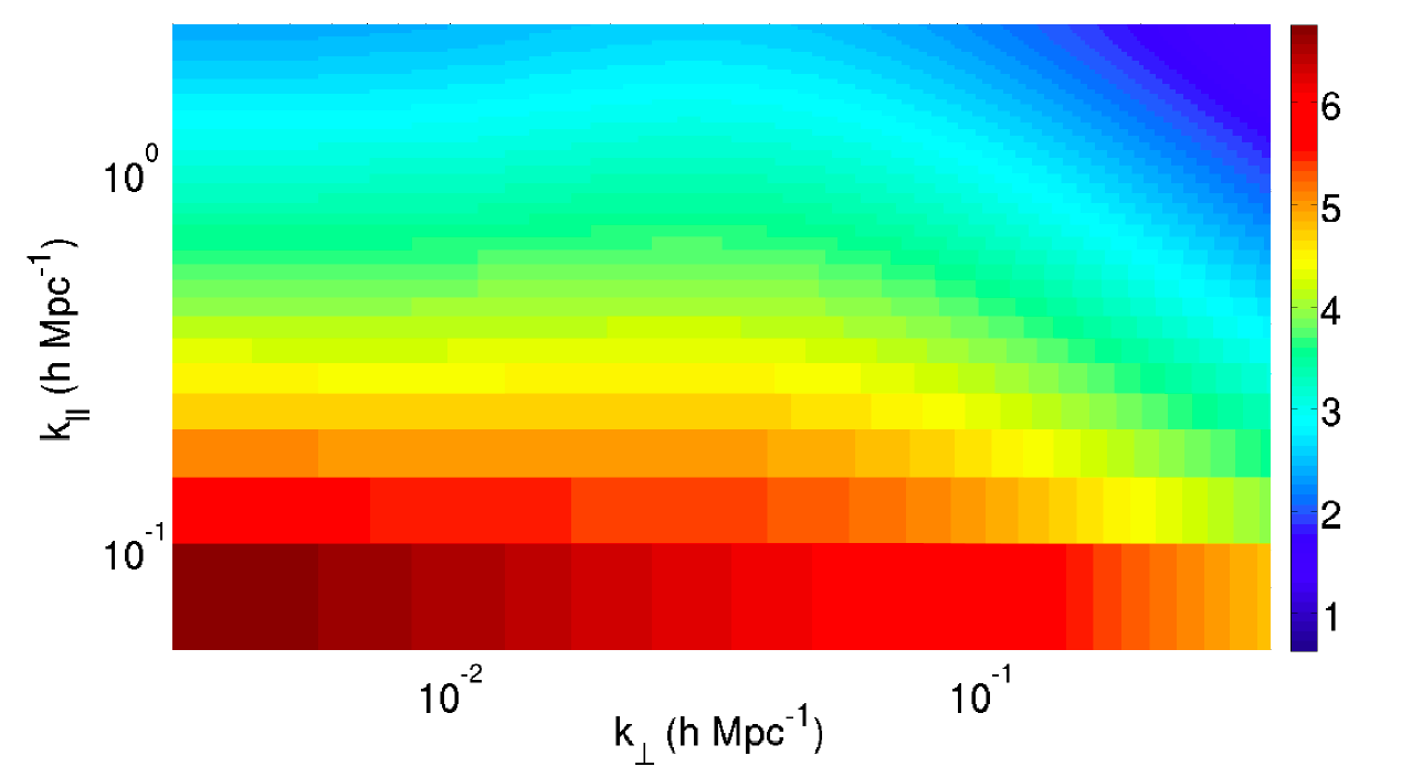
Figure 1.— Power spectra of the expected Cosmological HI signal. The power is plotted as $log_{10}P$ where P is in units $mK^{2}(Mpc/h)^{3}$.

Eqs. (15) and (10) can be used to infer many important properties of the HI signal:

• There exists a near one-to-one relation between u, $\tau$ and the Fourier components of the HI power spectrum (Parsons et al. (2012a, b); Paul & Sethi et al. (2014); Morales & Hewitt (2004)):

  $$u_{\nu}=\frac{k_{\perp 1}r_{\nu}}{2\pi},\hskip 10.0ptv_{\nu}=\frac{k_{\perp 2}r_{\nu}}{2\pi},\hskip 10.0pt\tau=\frac{k_{\parallel}c(1+z)^{2}}{2\pi H_{0}\nu_{21}E(z)}$$ (16)

  where $\nu_{21}$ is the rest frame frequency of the 21 cm line, $r_{\nu}$ is the transverse comoving distance, $E(z)=\sqrt{\Omega_{M}(1+z)^{3}+\Omega_{k}(1+z)^{2}+\Omega_{\Lambda}}$ and z is the redshift corresponding to the observed frequency $\nu$. The relation between $k_{\parallel}$ and $\tau$ follows from the relation: $2\pi\tau=k_{\parallel}dr_{\nu}/d\nu$ (Eq. (15)). As noted above, all the frequency dependent quantities in Eq. (16) are computed as a fixed frequency $\nu_{0}=154\,\rm MHz$.

• The correlations in the sky plane and along the line of sight are nearly separable. This allows us to compute weights in the plane of the sky owing to $w$-term and the distortion of intensity pattern in a tracking run (the next two subsections) without the additional complication owing to frequency dependence of these quantities.

• Eqs. (15) and (16) allow us to simplify the relation between visibility correlation and the HI power spectrum. Eq. (15) can be solved in the limit defined by Eq. (16) to give (e.g. Thyagarajan et al. (2015a); Pen et al. (2009); Morales (2005); McQuinn et al. (2006)):

  $$\langle V_{\tau}({\bf u})V_{\tau}^{*}({\bf u})\rangle={\bar{I_{\nu}}^{2}\Delta\nu\theta_{0}^{2}\over r_{\nu}^{2}dr_{\nu}/d\nu}P_{\rm HI}(k)$$ (17)

  Here the MWA primary beam solid angle $\theta_{0}^{2}=\lambda^{2}/A_{\rm eff}$. For MWA $A_{\rm eff}=21.5\,\rm m^{2}$ at 150 MHz (Tingay et al. (2013)). $\Delta\nu=10.2\,\rm MHz$ is the total band width we use in this work. The mean specific intensity ${\bar{I_{\nu}}}=2k_{B}T_{B}/\lambda^{2}$. This allows us to express the HI signal as the square of the product of mean brightness temperature and the HI power spectrum $T_{B}^{2}P_{\rm HI}(k)$ in the units $(mK)^{2}(Mpc/h)^{3}$. It should be emphasized that Eq. (17) provides the suitable normalization only when ${\bf u^{\prime}}={\bf u}$, $w=0$, as has been assumed throughout this section, and the impact of sky intensity distortion while tracking a region is not considered. All these effects act to lower the RHS of Eq. (17), the measured visibility correlation, for a fixed signal $T_{B}^{2}P_{\rm HI}(k)$. This is accounted for by appropriate weights we discuss in the next two sections.

2.1. HI signal and w-term

From Eqs. (14) and (15), we can gauge the impact of the $w$-term. These equations and the discussion following them shows that the angular integrals depend only weakly on the line of sight variables. The main effect of the $w$-term is to alter the integrals over angles which we study here.

For a given baseline ${\bf b}$: $w_{\nu}={\bf b}\cdot{\bf s}_{0}\nu/c$, where ${\bf s}_{0}$ is the phase center at any time. As a region is tracked, the $w$-term changes owing to the drift of the phase center. For a tracking run, ${\bf u}_{\nu}^{2}+w_{\nu}^{2}$ is left invariant at any frequency; this result simply follows from the fact the the baseline length is fixed.

After the inclusion of the $w$-term, the measured visibility for a given intensity distribution is given as:

$$V_{\nu}({\bf u}_{\nu},w_{\nu})=\int A_{\nu}(l,m)\Delta I_{\nu}(l,m)$$ (18)

$$\times \exp{\left[-i2\pi\left\{u_{\nu}l+v_{\nu}m-w_{\nu}/2(l^{2}+m^{2})\right\}\right]}dldm$$

Here we have replaced $\vec{\theta}$ with its components (l,m) and also made the approximation:$\sqrt{1-l^{2}-m^{2}}-1\simeq-(l^{2}+m^{2})/2$, which is valid for MWA primary beam. After substituting Eq. (4) into Eq. (18) gives us:

$$V_{\nu}({\bf u}_{\nu},w_{\nu})=\bar{I}_{\nu}\int\frac{d^{3}k}{(2\pi)^{3}}\delta_{\rm HI}({\vec{k}})e^{ir_{\nu}k_{\parallel}}\int A_{\nu}(l,m)$$

$$\times\exp\biggl{[}-2\pi i\biggl{\{}\left(u_{\nu}-\frac{{k_{\perp 1}}r_{\nu}}{2\pi}\right)l+\left(v_{\nu}-\frac{{k_{\perp 2}}r_{\nu}}{2\pi}\right)m$$

$$-{w_{\nu}\over 2}(l^{2}+m^{2})\biggl{\}}\biggl{]}dldm$$ (19)

Each MWA tile being approximately a square aperture, the primary beam $A_{\nu}(l,m)$ can be written as:

$$A_{\nu}(l,m)=\frac{\sin(\pi L_{x}l)}{\pi L_{x}l}\frac{\sin(\pi L_{y}m)}{\pi L_{y}m}$$ (20)

Here $L_{x}$ and $L_{y}$ are dimensionless. They correspond to the ratio of the length of the tile along x- and y-axis to the wavelength. For central wavelength of the observation $L_{x}=L_{y}\simeq 2$. Eqs (18) and (20) show that integrals over $l$ and $m$ are separable and identical. These integrals cannot be done analytically but under certain approximations meaningful analytic expressions can be found. Let us define:

$$Q_{\nu}(k_{\perp 1};u_{\nu},w_{\nu}) = \int dl\exp\biggl{[}-2\pi i\biggl{\{}\left(u_{\nu}-\frac{{k_{\perp 1}}r_{\nu}}{2\pi}\right)l$$ (21)

$$-{w_{\nu}\over 2}l^{2}\biggl{\}}\biggl{]}\frac{\sin(\pi L_{x}l)}{\pi L_{x}l}$$

$Q_{\nu}(k_{\perp 1};u_{\nu},w_{\nu})$ is a function of $k_{\perp 1}$ and is parametrized by $u_{\nu}$ and $w_{\nu}$. First we consider, $w=0$. In this case, it can be shown that if the limits of the integral are allowed to go from minus infinity to plus infinity, we obtain,

$$Q_{\nu}(k_{\perp 1};u_{\nu},0) = {1\over L_{x}}\,\,\>{\rm if}\,\,|(u_{\nu}-r_{\nu}k_{\perp 1}/(2\pi))|/L_{x}<1/2$$ (22)

$$= 0\,\,\>\hbox{otherwise}$$

We notice that the approximation used is good because the function has a compact support provided by the primary beam. As $L_{x}\simeq 1/\theta_{0}$ where $\theta_{0}$ is the extent of the primary beam, this result means that, for a given $u_{\nu}$, the wavenumbers that contribute to the integral are the ones that are bounded by the extent of the primary beam. This result is already implied by Eq. (14).

Eq. (21) cannot be analytically approximated so readily for non-zero $w$. We use the stationary phase approximation to analytically evaluate the integral. For this assumption to hold, the phase of the exponent should be much larger than the slow variation of the primary beam. This would be the case if $wl^{2}$ is large. In this approximation, we obtain:

$$Q_{\nu}(k_{\perp 1};u_{\nu}, w_{\nu})=\sqrt{{2i\over w}}{\sin(\pi L_{x}(u_{\nu}-k_{\perp 1}r_{\nu}/(2\pi))/w_{\nu})\over\pi L_{x}(u-k_{\perp 1}r_{\nu}/(2\pi))/w_{\nu}}$$ (23)

$$\times\exp\left[-i(u_{\nu}-k_{\perp 1}r_{\nu}/(2\pi))^{2}/(4\pi w_{\nu})\right]$$

The main impact of the inclusion of the $w$-term can be discerned from this expression. In the limit of large $w$, the impact of the $w$-term is to shrink the MWA beam and the primary beam tends to $1/\sqrt{w}$ (Cornwell et al. (2008)). However, this also means that the spread of $k_{\perp 1}$ for which the integral is non-zero also increases, as seen in the terms involving the $sin$ function. If the decrease of primary beam results in a loss of signal-to-noise, an increase in the correlation length $|{\bf u}-{\bf u^{\prime}}|$ gains signal-to-noise. We can write visibility correlation for pairs of ${\bf u},w$ and ${\bf u^{\prime}}_{\nu},w_{\nu}^{\prime}$ as:

$$\langle V_{\nu}({\bf u}_{\nu},w_{\nu})V_{\nu}^{*}({\bf u^{\prime}}_{\nu},w_{\nu}^{\prime})\rangle=\int{d^{3}k\over 2\pi^{3}}P_{\rm H1}(k)Q(k_{\perp 1};u_{\nu},w_{\nu})$$

$$\times Q(k_{\perp 2};v_{\nu},w_{\nu})Q(k_{\perp 1};u_{\nu}^{\prime},w_{\nu}^{\prime})Q(k_{\perp 2};u_{\nu}^{\prime},w_{\nu}^{\prime})$$ (24)

Eq. (24) can be computed numerically. In Figure 2, we show how the HI correlation function is affected in the presence of $w$-term. These expressions are also valid for diffuse foregrounds which have a different 2-dimensional power spectrum and frequency dependence, e.g. optically thin Synchrotron radiation for which the angular and frequency dependence is separable. As Eq. (24) can be used to compute the impact of $w$-term at any frequency, it can readily be generalized to study diffuse foregrounds.

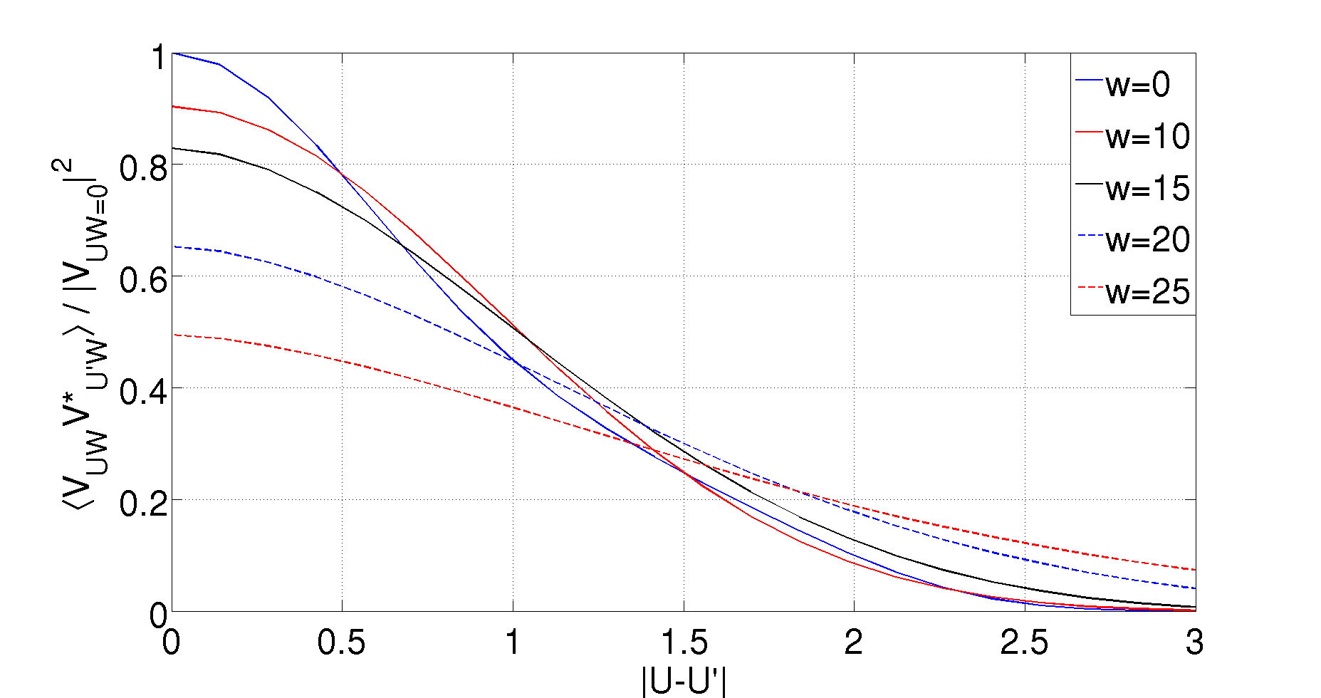
Figure 2.— The HI signal is plotted as a function $|{\bf u}-{\bf u^{\prime}}|$ for different values of w. The impact of w-term is to decrease the overall signal owing to shrinking of the primary beam and increase the correlation length $|{\bf u}-{\bf u^{\prime}}|$.

2.2. Time dependent coordinate system and w-term

In a tracking interferometric observation, a phase center is tracked and snapshots are taken at regular intervals with short duration. Each of these snapshots can be imaged and the images added if the successive fields of view can be assumed to be coplanar. This approximation breaks down for wide field-of-view instruments such as MWA. One manifestation of the wide field-of-view is the $w$-term whose impact was studied in the previous sub-section. In this section we generalize the discussion of the last sub-section to take into account the time dependence of the non-coplanarity of the tracked region (Perley (1999)).

As the region is tracked, the relation between the image and astronomical coordinates changes which distorts the intensity pattern with respect to the phase center being tracked. More specifically, this effect arises from the projection of a non-coplanar array on a plane, which is necessary to perform the Fourier transform for imaging. It is best illustrated with a set of point sources. These sources appear to move with respect to the phase center (e.g. Fig. 19-9 in Perley (1999)). The distortion of the intensity pattern corresponds to non-uniform stretching and it increases for sources further away from the phase center. Thus this effect can not be corrected by a standard shift of coordinate. The non-uniform stretching makes the situation complex, and the standard grid approach is difficult to implement in this case. For a set of point sources, the correction for this effect could be applied iteratively in the image plane (Chapter 19, Perley (1999)).

For a small field-of-view, this effect can be neglected and a unique coordinate system (e.g. time independent direction cosines $\{l,m\}$) can be used to relate the image coordinates with the sky intensity pattern for a long tracking run. However, it is not possible to define such a coordinate system when either the field of view is large or the tracking period is long.

Our aim here is not to correct for this effect but rather to estimate its impact on the correlation of visibilities at two different times during a tracking run: suppose we measure visibilities within a small cell in the $u$–$v$ plane (the size of the cell will be discussed in a later section) centered around a baseline $\{u,v\}$ at $t=0$. At a later time $t=t^{\prime}$ another baseline might enter this cell. From the discussion in the previous subsections (e.g. Figure 2) the two visibilities are expected to correlate strongly with each other (even if the values of $w$ differ significantly for these two sets this statement is generally true). However, visibilities measured at two different times do not correspond to the same intensity pattern. Our aim here is to estimate the level of de-correlation caused by the distortion of intensity pattern during a tracking run. In this paper, we construct a time-dependent coordinate system which allows us to analyse this distortion of intensity pattern. We assess the impact of this effect when a region is tracked using the MWA primary beam. In particular, we consider this effect on the visibilities produced by the EoR HI signal.

We start by recalling the definition of direction cosines for a point on the sky whose coordinates, declination and hour angle $\{\delta,h\}$, are: written as (Christiansen & Hogbom (1969)):

$$l = \sin(h)\cos(\delta)$$ (25)

$$m = \cos(\delta)\cos(h)\sin(\phi)-\sin(\delta)\cos(\phi)$$ (26)

$$n = \cos(\delta)\cos(h)\cos(\phi)+\sin(\delta)\sin(\phi)$$ (27)

It can be shown that $n=\sqrt{1-l^{2}-m^{2}}$. The phase center is always defined as $l=0$, $m=0$, $n=1$; for the coordinates defined above it is: $h=0$ and $\delta=\phi$.

As a phase center is tracked owing to the rotation of the Earth, $\delta$ remains fixed but the hour angle changes. For a wide field of view, this can result in distortion of the intensity pattern of the sky. To take into account this effect, we can define a time-dependent coordinate system:

$$l(\delta h)=\sin(h+\delta h)\cos(\delta)-\sin(h_{0}+\delta h)\cos(\delta_{0})$$ (28)

Here $h_{0}$ and $\delta_{0}$ define the phase center for $\delta h=0$; $\delta h$ defines the flow of time. $m$ can be similarly defined and $n$ can be computed from $l$ and $m$. This definition gives a time dependent coordinate system where the coordinates are always defined with respect to the phase center. It is easy to verify that for small field of view and for small tracking times, which corresponds to cases when higher order terms in $h$, $\delta h$ and $\delta$ can be dropped, $l$ is independent of time which means that the distance of a point from the phase center is left invariant under tracking. In such cases, the intensity pattern on the sky corresponds to the unique intensity pattern defined by sky coordinates $\delta$ and $h$ and remains unchanged as the phase center is tracked.

However, when this approximation breaks down, $l$ becomes a function of time and it is impossible to define a unique relation between direction cosines and sky coordinates. This means that any quantities defined with respect sky coordinate (e.g. intensity pattern) become time dependent. The visibility for the HI signal is given by:

$$V_{\nu}({\bf u}_{\nu},w_{\nu},\delta h)=\bar{I}_{\nu}\int\frac{d^{3}k}{(2\pi)^{3}}\delta_{\rm HI}({\vec{k}})e^{ir_{\nu}k_{\parallel}}\int A_{\nu}(l,m)$$

$$\times\exp\biggl{[}-2\pi i\biggl{\{}\left(u_{\nu}-\frac{{k_{\perp 1}}r_{\nu}}{2\pi}\right)l+\left(v_{\nu}-\frac{{k_{\perp 2}}r_{\nu}}{2\pi}\right)m$$

$$-{w_{\nu}\over 2}(l^{2}+m^{2})\biggl{\}}\biggl{]}\sin\delta d\delta dh$$ (29)

The direction cosines $l$ and $m$ are now functions of time. The angular integral is carried out over $\delta$ and $h$. Unlike the earlier case (fixed grid) this is not a product of two one-dimensional integrals. The correlation of the visibilities $V_{\nu}({\bf u}_{\nu},w_{\nu},\delta h)$ can be computed using the same methods as outlined in the previous sections.

In Figure 3 we show the results when the effect of the time dependent coordinate system (’moving grid’) is included. The initial phase center ($\delta h=0$) is chosen to be $h=0$ and $\delta=\phi$. The results are shown for two different values of $\delta h$ and a range of $w$ values. We only show the auto-correlation function for a given value of $\delta h$. But the results shown in Figure 3 can be used to assess the cross-correlation of visibilities measured at two different times. For our case the value of this cross-correlation lies between the auto-correlations of visibilities measured at the same time. The moving grid doesn’t introduce another scale in the problem and the results in this case are not very different from the case for a fixed grid. In both cases the dominant correlations occur for ${\bf u}-{\bf u^{\prime}}<1.5$.

Figures 2 and 3 are based on MWA primary beam. However, it is possible to glean generic information applicable for other primary beams from them. First, the decorrelation length $|{\bf u}-{\bf u^{\prime}}|$ scales as the inverse of the primary beam (e.g. Paul & Sethi et al. (2014)). So for a smaller beam, the decorrelation seen in the Figures as a function of $|{\bf u}-{\bf u^{\prime}}|$ would be shallower. The impact of the $w$-term for a different primary beam can be partially gauged from Eq. (23), which is valid for large values of $w$. In this limit, the primary beam tends to $1/\sqrt{w}$, irrespective of the primary beam of the telescope. It is difficult to analytically estimate the impact of the $w$-term when this limit does not hold. But it can be shown that the impact of $w$-term diminishes for a smaller primary beam, e.g. a Gaussian beam for which the primary beam tends to $(1/\theta_{0}^{2}+\pi w_{\nu})^{-1/2}$ for non-zero $w$ (e.g. Paul & Sethi et al. (2014)). As noted above, the distortion of intensity pattern during a tracking run is a wide field effect. For a smaller primary beam, the level of decorrelation seen in Figure 3 would be smaller but it is difficult to analytically estimate it.

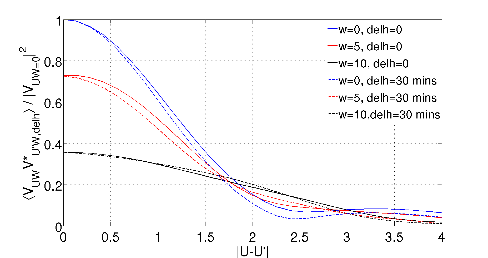
Figure 3.— The HI signal is plotted as a function $|{\bf u}-{\bf u^{\prime}}|$ for different values of w and $\delta h$. The initial phase center is chosen to be $h=0$ and $\delta=\phi$.

2.3. Weights for cross-correlation

Eq. (29) can be used to compute the counterpart of Eq. (14) which takes into account the impact of non-zero $w$-term and the distortion of intensity pattern. We compute this expression for the visibility correlation in delay space numerically. In this formulation, the measured visibility is a function of five parameters: $\tau,{\bf u},w,t$. Here, as noted above, ${\bf u}$ and $w$ are the values of these variables at a fixed frequency which we choose to be $\nu_{0}=154\,\rm MHz$.

We define the weight on a given cross-correlation as:

$${\cal W}({\bf u},w,t;{\bf u^{\prime}},w^{\prime},t^{\prime})={\langle V_{\tau}({\bf u},w,t)V_{\tau}^{*}({\bf u^{\prime}},w^{\prime},t^{\prime})\rangle\over\langle V_{\tau}({\bf u},0,t)V_{\tau}^{*}({\bf u^{\prime}},0,t^{\prime})\rangle}$$ (30)

The weights are defined with respect to the HI cross-correlation computed in Eq. (14) for ${\bf u}={\bf u^{\prime}}$, $w=w^{\prime}=0$, $t=t^{\prime}$ and $\tau=\tau^{\prime}$. We only consider the case $\tau^{\prime}=\tau$ for the computation of weights.

Using Eq. (30) allows one to recover the HI power spectrum for a fixed wave number $k$ from visibility cross-correlations.

3. Analysis of MWA data

The MWA is a low frequency radio interferometer array located in Western Australia. It consists of 128 antenna tiles with each tile comprising of 16 crossed dipole antennas over a metal ground screen in 4 x 4 grid. MWA bandwidth is 30.72 MHz, divided into 24 coarse channels of width 1.28 MHz each. The total bandwidth is divided into 768 fine channels. With the use of an analog beamformer appropriate phase delays are introduced in each individual dipole antenna to track the pointing center of the beam across the sky. For more information on MWA please see Tingay et al. (2013); Lonsdale et al. (2009).

To minimize the effect of Galactic synchrotron emission, the MWA EoR community has chosen three fields on the sky away from the Galactic plane. These fields have been named as EoR0, EoR1 and EoR2 and are shown in Figure 4. In this paper we present 3 hours of tracking analysis of the EoR1 field centered at RA $=$ 4h, Dec $=-27^{\circ}$.

Many research groups are currently developing pipelines to extract statistical information from radio interferometric data, with an aim to detect the HI signal from EoR (Jacobs et al. (2016); Hazelton et al. (2016); Dillon et al. (2015); Trott et al. (2016)). These can be divided broadly into two categories: image based and visibility based pipelines. For foreground subtraction and imaging these pipelines use the following imaging algorithms: Real Time System (RTS; Mitchell et al. (2008); Ord et al. (2010)) and Fast Holographic Deconvolution (FHD, Sullivan et al. (2012)).

The image based pipelines (Dillon et al. (2015); Hazelton et al. (2016)) use source catalog created through the deconvolution of the data which is subtracted to obtain a residual image cube. The Fourier transform of this image cube with some further processing yields the power spectra. On the other hand, the visibility based pipelines (Trott et al. (2016)) use the data in visibility domain for power spectra estimation, after the initial processing in the image domain for obtaining the foreground model. The detailed comparison of the outputs from all the methods described above is provided in Jacobs et al. (2016). Thyagarajan et al. (2015a, b) describe the impact of wide field of view in power spectra estimation.

A special variant among the visibility based estimators is ‘delay spectrum’ (Pober et al. (2013); Parsons et al. (2012b, 2014)), which directly Fourier transforms each calibrated visibility along its frequency channels. The radio interferometer PAPER uses this approach extensively; it relies upon redundant baselines to calibrate the interferometer and East-West and near East-West baselines for power spectrum estimation (Parsons et al. (2012b, 2014); Ali et al. (2015)). This particular scheme has been discussed and implemented only for redundant drift scan observations. In this paper we explore the possibility of applying this approach for non-redundant imaging arrays and tracking measurements.

In this and the next section, we discuss in detail our method of MWA data analysis and power spectrum estimation from the data.

We summarize below the major ingredients of the method and then describe each of the stpng in detail in subsequent sections:

• CASA (McMullin et al. (2007)) is used for initial processing of the data to calibrate raw visibility measurements. This is followed by the creation of a model sky image from clean components. This model is then subtracted in the visibility domain to obtain residual visibilities. We use both the calibrated and residual visibilities for computing the power spectrum.

• Each visibility is then Fourier transformed in frequency space (Eq. (31)). This process is needed for isolation of foregrounds in the $k_{\perp}\hbox{--}k_{\parallel}$ plane. We note the our method utilizes both the subtraction of foregrounds and their isolation. But it does not employ an external point source catalog.

• The procedure outlined above yields complex visibilities as a function of five variables: $V_{\tau}(u,v,w,t)$. For computing the power spectrum we cross-correlate these visibilities for $t^{\prime}\neq t$ to remove the noise bias. To weigh each cross-correlation we assume that there exist regions in $k_{\perp}\hbox{--}k_{\parallel}$ plane which are dominated by only noise and the HI signal. This allows us to compute a weight for each cross-correlation based on the expected HI signal. For computing these weights we take into account the impact of $w$-term and the distortion of intensity pattern in a tracking scan. The relevant method is elaborated in detail in sections 2, 2.1, 2.2, and 2.3 and summarized in section 4.

• In section 4.1, we describe the power spectrum estimator, taking into account weights given by the expected HI signal, in 3-, 2- and 1-dimension. We also discuss our method to compute the errors on the estimated power spectrum.

3.1. CASA processing

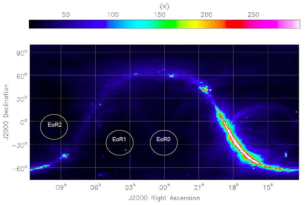
Figure 4.— EoR fields are shown on the Galactic map at 408 MHz (Haslam et al. (1982)). Three fields, away from the galactic plane, have been identified for the MWA reionization study. These are EoR0, EoR1 & EoR2 respectively as shown in circles. In this paper we focus on the EoR1 field centered at RA $=$ 4h, Dec $=-27^{\circ}$.

MWA data were collected at 2-minute intervals with a time resolution of 0.5 seconds and frequency resolution of 40 kHz. The central frequency of these observations is 154.24 MHz. For preprocessing we have used the Cotter pipeline (Offringa et al. (2015)) to average to 10 seconds of integration; we have not performed any averaging over the frequency channels. Cotter also uses the in-built AOFlagger to flag and remove radio frequency interference. The edge channels of each coarse band are flagged with Cotter due to aliasing effects. After this preprocessing the Cotter pipeline delivers the data in the CASA readable ‘Measurement set (ms)’ format for further processing.

Once the ‘ms’ files are produced for each 2-minute data set, we process each of these 2-minute data in CASA to produce an image. The Hydra A source is used to calculate the bandpass solutions which are applied to the uncalibrated data. We next construct a sky model from these data so that we could subtract it to obtain the residual visibility. After the bandpass calibration the first round of ‘clean’ is applied on each 2-minute data set. The multi-scale multi-frequency synthesis algorithm (Rau & Cornwell (2011)) has been used for imaging. We have created images of size 3072 x 3072 pixels with 1 arc-minute cell size using the Cotton-Schwab CLEAN (Schwab (1984)) with uniform weighting scheme. After the first round of clean we have performed self calibration (both phase and amplitude+phase) and apply the clean loop until the RMS value of the residual image converges. The threshold limits for the clean stpng were chosen to be 5 sigma. The W-projection algorithm (Cornwell et al. (2008)) was also used to correct for the errors arising due to non-coplanarity of baselines. Once we obtain the best model of the sky for each 2 minute observation, the model visibilities are then subtracted from the calibrated data using the UVSUB algorithm in CASA to obtain the residual data. This process is followed for both XX & YY polarizations separately. A flow chart of the data pipeline is shown in Figure 5. In Figure 6, we present a sample image of 2 minute deconvolution.

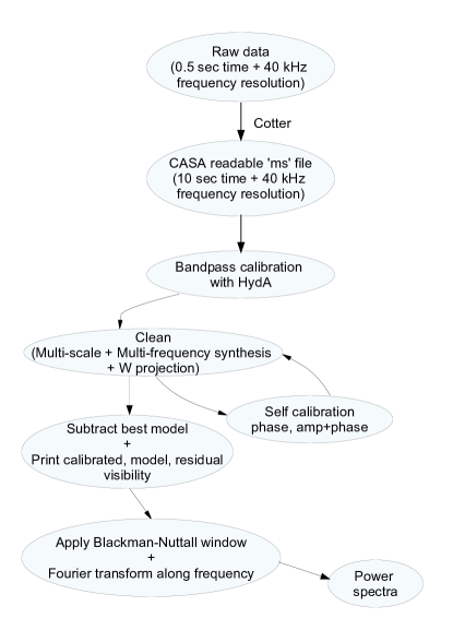
Figure 5.— A schematic of the power spectra pipeline is shown.

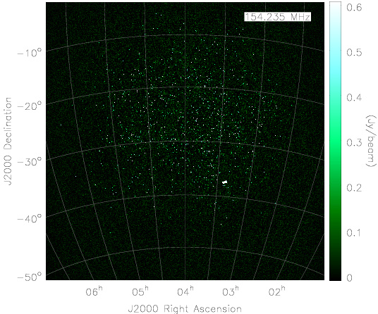
(a)

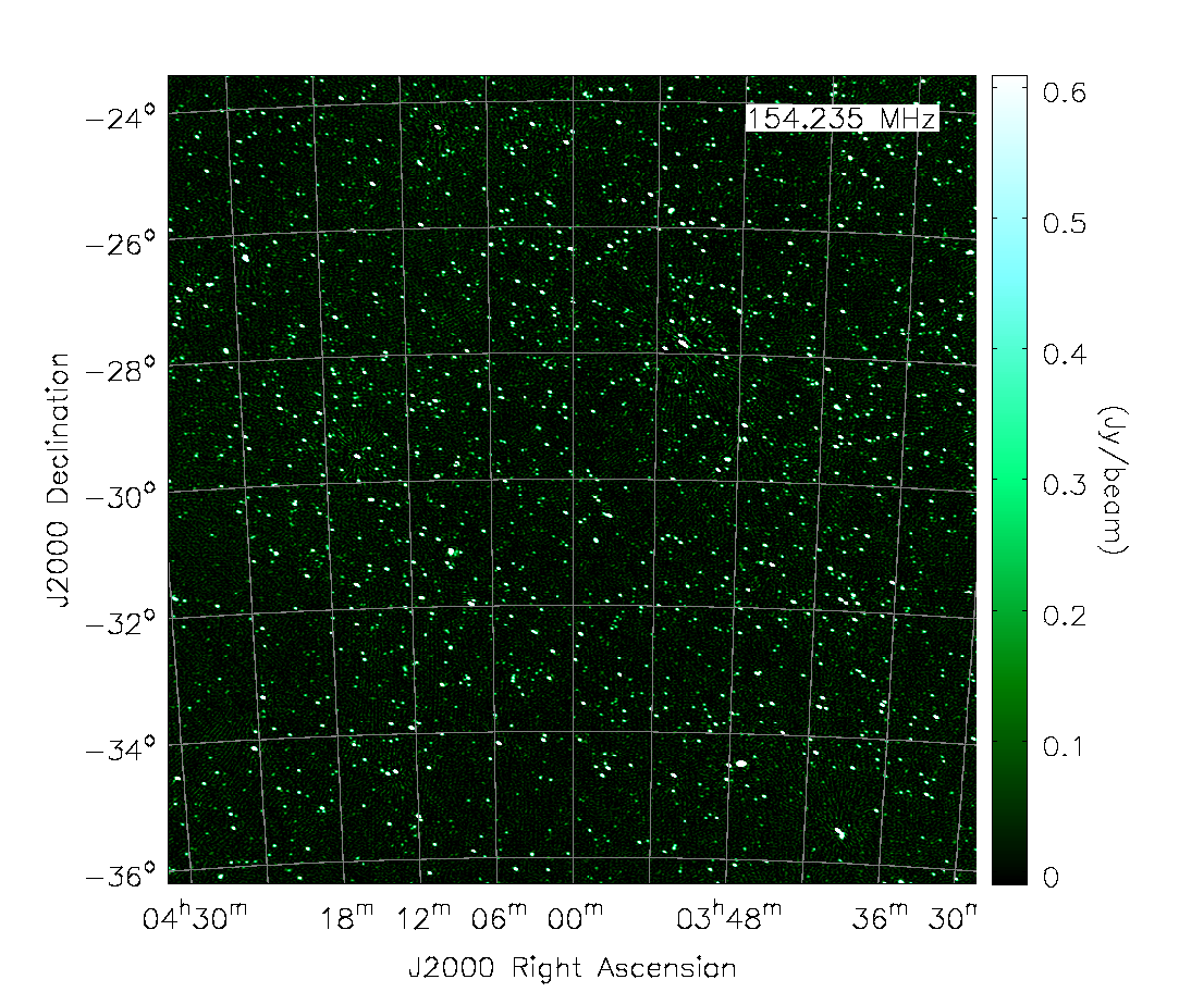
(b)

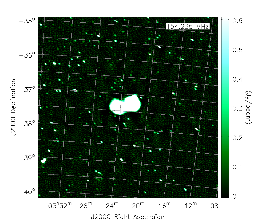
(c)

Figure 6.— The image of EoR1 field at 154.24 MHz is shown in the top panel for two minutes of data. The bottom panels display two regions from the image. The right panel displays the region containing the Fornax A.

As noted above we process the data for only 2 minutes to ensure the primary beam doesn’t substantially change during the run. For a 2-minute scan we obtain an RMS of nearly 40 mJy/beam.

The residual visibility $V_{\nu}(u_{\nu},v_{\nu},w_{\nu},t)$ is a function of five variables. We compute the discrete Fourier transform of the residual visibilities in the frequency space weighted by the Blackman-Nuttall (Nuttall (1981)) window $B_{\nu}$ to suppress leakage into the EoR window (Thyagarajan et al. (2013, 2016)):

$$V_{\tau}(u,v,w,t)=\sum\Delta\exp(i2\pi\nu\tau)V_{\nu}(u_{\nu},v_{\nu},w_{\nu},t)B_{\nu}$$ (31)

Notice that in Eq. (31) the frequency dependence of the baseline vector ${\bf b}_{\nu}=\{u_{\nu},v_{\nu},w_{\nu}\}$ is integrated over. Therefore, the labels $\{u,v,w\}$ on the LHS of Eq. (31) need further explanation. As noted above (the discussion following Eq. (11)) they can be chosen to denote a given baseline vector at a fixed frequency, $\nu_{0}$. We choose this frequency to be the central frequency of the band $\nu_{0}=154\,\rm MHz$. Parsons et al. (2012a, b) provide detail implications of the frequency dependence of the baseline vector. Here $\Delta=40\,\rm kHz$ and 256 channels are used for our study, which correspond to total bandwidth 10.24 MHz in the frequency range 149.09 MHz to 159.34 MHz.

4. Power spectrum

The visibilities (Eq. 31) are cross-correlated with weights determined from the HI signal (section 2.3) to estimate the power spectrum. For each pair of parameters, e.g. $\{u,u^{\prime}\}$, the weights are generally different. It is computationally prohibitive to deal with weights for all cross-correlations. We make several simplifying assumptions to make the problem tractable based on the properties of the HI signal. In sections 2, 2.1, and 2.2 we discuss in detail the HI signal and how it is affected by the inclusion of the $w$-term and the additional complication arising from distortion of the field of view as a region is tracked for MWA.

We summarize the main results of these sections as applied to the data:

• In section 2 the HI signal and its correlations are discussed in detail. Eq. (15) shows that correlations in sky plane are nearly independent of correlations along the line of sight. This allows us to compute weights for correlations in the plane of the sky independent of the third axis. Eq. (15) allows us to derive a relation between the measured correlation and the inferred HI power spectrum (Eq. 17). Eq. (17) defines the scale of cross-correlation weights. The weight function ${\cal W}(u,v,w,t;u^{\prime},v^{\prime},w^{\prime},t^{\prime})$ is unity when ${\bf u}={\bf u^{\prime}}$, $w=w^{\prime}=0$ and $t\simeq t^{\prime}$. Eq. (17) refers to this case.

• In section 2.1, the impact of $w$-term on the HI signal is computed. Eq. (23) and Figure 2 capture the effect of non-zero $w$ on HI correlations. The $w$-term diminishes the signal by shrinking the effective primary beam and increases the correlation length scale $|{\bf u}-{\bf u^{\prime}}|$. We use the analytic expression based on Eq. (23) for computing weights for $w>30$.

• In section 2.2, we attempt to assess the impact of time-dependent distortion of intensity pattern in a tracking run for MWA. Figure 3 shows the combined effect of moving grid and $w$-term. The distortion of intensity pattern generally acts to enhance decorrelation but is found to be not significant and doesn’t alter the main features of the signal. For our computation, we only update the weights after every 10 minutes to account for this effect.

4.1. Power spectrum estimator

As shown above each correlation receives a different weight depending on the values of $\{u,v,w,t\}$ of the baselines being correlated. As noted above, we define the weights ${\cal W}(u,v,w,t;u^{\prime},v^{\prime},w^{\prime},t^{\prime})$ such that they approach unity when $u=u^{\prime}$, $v=v^{\prime}$, $w=w^{\prime}=0$ and $t\simeq t^{\prime}$ such that the effect of the moving grid is not important ($t\neq t^{\prime}$ for all correlations to remove noise bias).

The HI power spectrum is a function of $k=\sqrt{{\bf k}_{\perp}^{2}+k_{\parallel}^{2}}$; Eq. (16) gives the relation between the Fourier components of the HI signal and $\{{\bf u},\tau\}$. All cross correlations for which the wave vector lies in some range $k$ and $k+dk$ can be used to construct the unbiased HI signal: $1/N\sum V_{\tau}(u,v,w,t)V_{\tau^{\prime}}(u^{\prime},v^{\prime},w^{\prime},t^{\prime})/{\cal W}$; here $N$ is the number of all pairs for which $k$ lies in the range specified above. However, this estimator, though unbiased for the HI signal, could be dominated by small values of weights ${\cal W}$, which doesn’t make it the lowest noise (or optimal) estimator.

As the observed signal is dominated by noise, we consider an optimal estimator for our study:

$$\hat{P}_{\tau}(u,v)={1\over\sigma}\sum_{u^{\prime},v^{\prime},w,w^{\prime},t,t^{\prime}}\left(V_{\tau}V_{\tau}^{*}\times{\cal W}\right)$$ (32)

where $\sigma=\sum_{u^{\prime},v^{\prime},w,w^{\prime},t,t^{\prime}}{\cal W}^{2}(u,v,w,t,u^{\prime},v^{\prime},w^{\prime},t^{\prime})$. To avoid noise bias, $t\neq t^{\prime}$ for all cross-correlation. For a given $\{u,v,\tau\}$, Eq. (32) allows us to compute the power spectrum by optimally weighing over all the cross correlations. However, as Figures 2 and 3 show the correlations fall substantially for ${\bf u}-{\bf u^{\prime}}\geq 1.5$ (see also Paul & Sethi et al. (2014) and references therein). This motivates us to pixelize the ${\bf u}$-plane and consider only those visibility pairs for which the correlations are significant. We consider cells of different sizes and present results here for $\Delta u=\Delta v=0.5$. The number of visibility measurements in a cell vary depending on the (u,v) values. The shortest baselines have higher population as expected for MWA. For 3 hours of analysis and $u,v<50$, the number of visibilities in a cell lie in the range $\sim 1000\hbox{--}3500$ where each visibility has a time resolution of $\Delta t=10$ sec. All the cross-correlation within a cell are computed using Eq. (32).

For averaging over different cells, each cell is assigned an average weight corresponding to the RMS of the power spectrum for a cell, $\sigma_{p}$. These weights are then used for optimally averaging the power spectrum (Eq. (32)) over other cells (For details see Appendix B). Note that this procedure allows us to separate large correlations of the HI signal, the ones for which ${\cal W}$ is close to unity, from the ones which are expected to be incoherent because ${\cal W}$ is small.

The schematic of the two processes—the computation of power spectrum in 3- and 2-dimensions—is displayed in figure (7): the top panel delineates the process of computing cross-correlations within each cell and the bottom panel depicts how azimuthal average for a fixed baseline length $\sqrt{u^{2}+v^{2}}$ is computed. For MWA data, $k_{\parallel}\gg{\bf k}_{\perp}$, which means the value of $k$ is dominated by the value of $k_{\parallel}$. This suggests the following method for computing the 1-dimensional power spectrum, which we adopt: all the cells for a given $\tau$ are optimally averaged using the method described above. This procedure yields a complex number. In the Figures that display 2- and 1-d power spectra we plot the absolute value of the estimated power spectrum.

(a)

(b)

Figure 7.— (a)This shows the population of visibilities within different uv bins for each $\tau$. The small dots denote visibilities due to individual baselines. These are cross-correlated with each other within a given uv bin. (b) The black dots within a bin are the power value at each bin. An optimal azimuthal average, based on weights of each cell, is done to collapse the uv axes into a single axis of baseline length.

The error on power spectrum in 1-dimension is computed by first estimating the RMS for each cell, $\sigma_{p}$. $\sigma_{p}$ are then used as weights for optimal averaging over all the cells for a fixed $\tau$. The resultant RMS after averaging over the cells approaches $\sigma_{\rm fin}\simeq(1/\sum\sigma_{p}^{2})^{-1/2}$ if the power spectrum across cells is uncorrelated. This holds for noise but, as noted above, is an approximation for the HI signal. We expect this assumption to be valid in our case as the observed signal is dominated by noise (for detailed explanation see Appendix B).

5. Results

In Figure 8, the power spectra computed from 3 hours of data are shown in the $k_{\perp}\hbox{--}k_{\parallel}$ plane. The power spectra for both XX and YY polarization are shown for calibrated and residual visibilities.

(a) dirty XX

(b) dirty YY

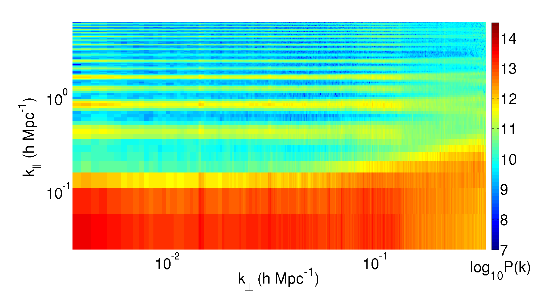
(c) residual XX

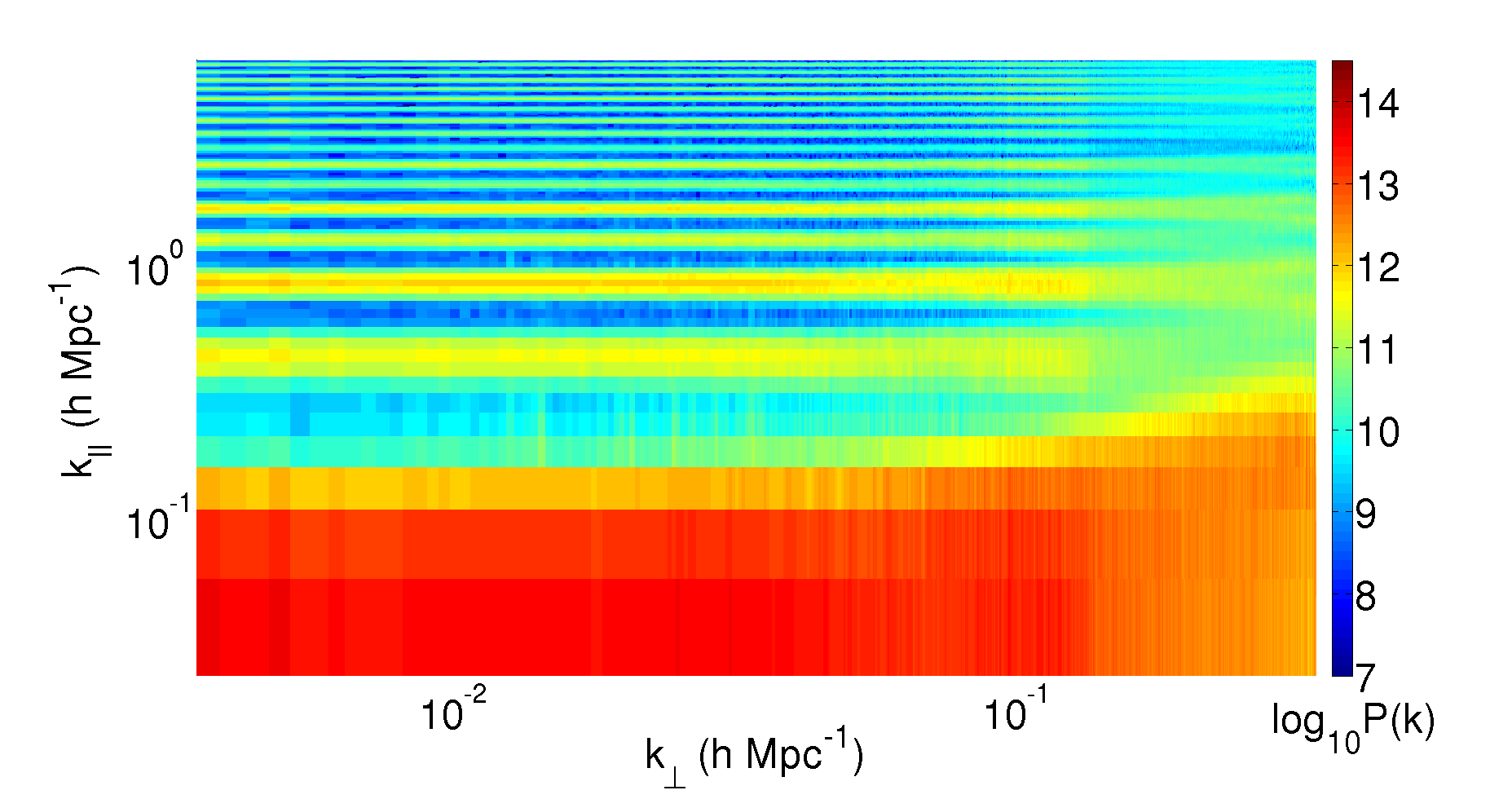
(d) residual YY

Figure 8.— Two-dimensional power spectra for 3 hrs of data on the EoR1 field for XX & YY polarization. The power is plotted as $log_{10}P$ where P is in units $mK^{2}(Mpc/h)^{3}$.

(a) XX

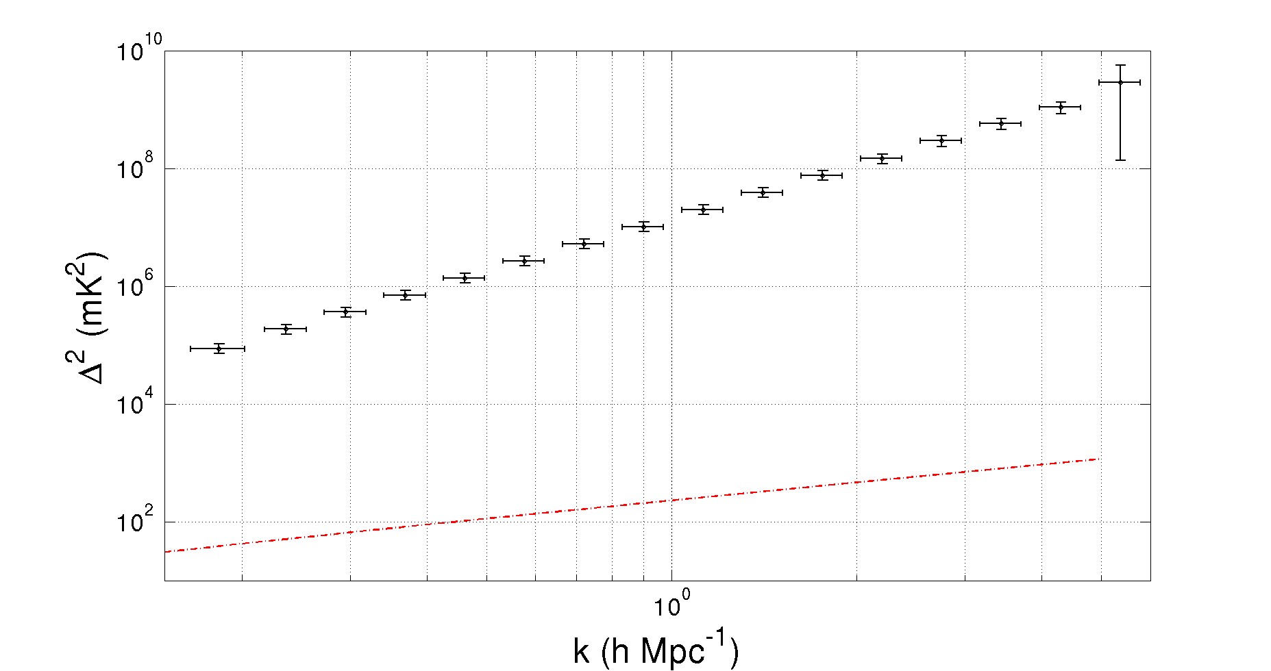
(b) YY

Figure 9.— One dimensional power spectra ($\Delta^{2}=k^{3}P(k)/(2\pi^{2})$ in units $(mK)^{2}$) for the XX (Left panel) and YY (Right panel) polarization are shown along with the errors for each band. The dot-dashed (red) curve show the expected HI signal (Furlanetto et al. (2006)).

We first discuss discernible features in the power spectra:

• In Fourier space the foreground contributions occupy a wedge shaped region (also called ‘foreground wedge’) owing to the smooth spectral characteristics of foreground sources (Datta et al. (2010); Vedantham et al. (2012); Parsons et al. (2012b); Liu et al. (2014a); Dillon et al. (2014); Thyagarajan et al. (2013, 2015a)). The region beyond the foreground wedge is expected to be free from the foreground contamination and dominated by thermal noise and expected HI signal. This foreground isolation approach is particularly useful for the MWA as it has low angular resolution. The strongest HI signals lie in the shortest baselines (low $k_{\perp}$ values) and it decreases rapidly with increasing $k_{\perp}$ values.

  The upper and lower panels of Figure 8 display the dirty (calibrated with no foreground subtraction) and the residual (clean components subtracted) power spectra, respectively. The Figure 8 bear out the assumption that foregrounds have smooth spectral characteristics as they are seen to form the ‘foreground wedge’, this separation is in good agreement with the expectation from foreground simulations (Figure 10). The first few $k_{\parallel}$ modes exhibit maximum foreground contributions, the $k_{\parallel}=0$ mode being the strongest. The amplitude at this mode is roughly $10^{14}\hbox{--}10^{15}\,\rm mk^{2}\,(Mpc/h)^{3}$ which is in good agreement with the results of other MWA EoR pipelines (Jacobs et al. (2016)). A clear decrement in power in the ‘foreground wedge’ is visible in residual power spectra as compared to the dirty one.

• As described in the previous section, MWA has missing channels on either side of coarse bands of width 1.28 MHz. This leads to a periodicity of missing data across the frequency axis in visibility, the effect of which is reflected in the Fourier-transformed power spectra as the horizontal bright lines at fixed $k_{\parallel}$.

Figure 9 shows the 1-dimensional power spectra; the 1-dimensional power spectrum is obtained from regions that exclude the foreground wedge and bright coarse bands in Figure 8. For computing the 1-d power spectrum, the foreground wedge and the bright coarse horizontal bands of the 2-d power spectrum (Figure 8) are rejected. More specifically, the channels corresponding to $k_{\parallel}\leq 0.14hMpc^{-1}$ and $k_{\perp}>0.1hMpc^{-1}$ are not considered. For each coarse band, the central brightest channel along with two channels on either side are excluded. The remaining contiguous regions are used in estimation of the 1-d power spectrum. For instance, for a given $k_{\parallel}$ that meets the criterion outlined above, all the cells that correspond to $k_{\perp}<0.1hMpc^{-1}$ are used for the computation of 1-d power spectrum. The error on the binned power spectra are computed using a scheme outlined in Appendix B.

The 2-d power spectra obtained from data (Figure 8) can be compared with Figure 10 that shows the expected power spectrum based on simulations of foregrounds and noise. In particular, this comparison allows us to assess the structure of coarse channels and the foreground wedge. It also indicates the range of scales of the 2-d power spectrum. However, Figure 10 is based on a single realization of noise and a model of foregrounds based on random distribution of point sources, and therefore a more detailed comparison between the data and simulations is not possible. We shall return to this detailed comparison in future work.

6. Conclusions

In this paper, we propose a new method to extract the HI power spectrum from MWA visibility data in delay space. The proposed method is applicable when a region is tracked using imaging radio interferometers.

One of the crucial factors in power spectrum estimation is how the $w$-term is dealt with within the pipeline. Our findings are that the $w$-term causes an effective shrinking of primary beam which reduces the contribution of the HI signal. We carefully model the HI signal by taking the $w$-term into account, the weights calculated are then applied to cross-correlate the measured visibilities. Moreover, the cross-correlation approach is particularly useful to minimize various systematics in the system. We also model and account for the impact of changing intensity pattern in a tracking run. We find this effect to be sub-dominant to the $w$-term correction.

We analyse three hours of MWA data from the EoR1 field, one of the field identified by the MWA community for EoR science. CASA has been used for calibration and to create foreground model using the clean components. Both the dirty (calibrated with no foreground subtraction) & residual (foreground model subtracted) power spectrum in delay space are presented. Our results (Figures 8 and 9) are in good agreement with the analyses of other MWA EoR pipelines (Jacobs et al. (2016)).

In the future we plan to apply the method proposed here for more integration time and, in particular, to a longer single tracking run. The decorrelation caused by the $w$-term and the changing intensity pattern would be more dominant in the latter case. This will allow us to test the efficacy of our method for more extreme cases and might indicate the best possible way of detecting the HI signal from the epoch of reionization.

7. Acknowlegements

We thank the referee for useful comments which helped us to improve the paper.

This scientific work makes use of the Murchison Radio-astronomy Observatory, operated by CSIRO. We acknowledge the Wajarri Yamatji people as the traditional owners of the Observatory site. Support for the operation of the MWA is provided by the Australian Government Department of Industry and Science and Department of Education (National Collaborative Research Infrastructure Strategy: NCRIS), under a contract to Curtin University administered by Astronomy Australia Limited. We acknowledge the iVEC Petabyte Data Store and the Initiative in Innovative Computing and the CUDA Center for Excellence sponsored by NVIDIA at Harvard University.

Appendix A Appendix A: Foregrounds and noise simulations

The primary contribution to foregrounds come from spectrally smooth point and diffuse sources. They differ from the HI signal in both spatial and spectral behaviour. However, it is the latter difference that allows us to potentially isolate foregrounds from the HI signal in the power spectrum estimation.

To understand the impact of foregrounds in the data, we model them as a set of point sources. We note that if both the point and the diffuse sources have smooth spectra across the instrumental bandwidth, their impact on the power spectra are similar and therefore point sources allow us to capture adequately our ability to isolate foregrounds from the signal. In this section, for analytic work, we assume $w=0$. We note without further proof that this assumption doesn’t alter our main inferences.

For a set of point sources, the intensity distribution is given by:

$$I_{\nu}({\vec{\theta}})=\sum_{i}F_{i\nu}\delta_{\scriptscriptstyle D}^{2}({\vec{\theta}}-{\vec{\theta}_{i}})$$ (A1)

Here $F_{i\nu}$ and ${\vec{\theta}_{i}}$ are the source fluxes and positions, respectively. This allows us to compute the visibility for a given baseline ${\bf u}_{\nu}$ and frequency $\nu$.

$$V_{\nu}({\bf u}_{\nu})=\sum_{i}F_{i\nu}\exp(i2\pi{\bf u}_{\nu}.{\vec{\theta}_{i}})A_{\nu}({\vec{\theta}_{i}})$$ (A2)

Here $A_{\nu}$ is the primary beam. As discussed earlier, we also define a visibility in the conjugate space by taking the Fourier transform with respect to $\nu$ (Eq. (11)): $V_{\tau}({\bf u})$. Our aim is to compute the correlation of this visibility:

$$\langle V_{\tau}({\bf u})V_{\tau^{\prime}}^{*}({\bf u^{\prime}})\rangle=\sum_{i}\sum_{j}\int d\nu\int d\nu^{\prime}F_{i\nu}F_{j\nu^{\prime}}\exp\left(i2\pi\left[{\bf u}_{\nu}.\vec{\theta}_{i}-{\bf u}^{\prime}_{\nu^{\prime}}.\vec{\theta}_{j}+(\tau\nu-\tau^{\prime}\nu^{\prime})\right]\right)A_{\nu}(\vec{\theta}_{i})A_{\nu^{\prime}}(\vec{\theta}_{j})$$ (A3)

Both the source flux $F_{\nu}$ and primary beam $A_{\nu}(\vec{\theta})$ are functions of frequency so it is difficult to analytically compute this expression. However, assuming smooth and small variation of both of these quantities across the bandwidth, we can make meaningful analytic estimates; we verify this assumption from detailed simulations and the analysis of the data. The main frequency variation in this case comes from the phase of the integral (the terms in the exponent) and in particular from the change in the baseline length as frequency changes. We note here that multiple correlations are available to us for this analysis for different pairs of $\{\tau,\tau^{\prime}\}$ and $\{{\bf u},{\bf u^{\prime}}\}$. Here we assume $\tau=\tau^{\prime}$.

Delay space—foreground wedge: Here we expand the same baseline in frequency space: ${\bf u^{\prime}}_{\nu^{\prime}}={\bf u}_{\nu}+d{\bf u}_{\nu}/d\nu(\nu^{\prime}-\nu)$. In this case, ${\bf u}_{\nu}=\nu/\nu_{0}{\bf u}_{\nu_{0}}$, where $\nu_{0}$ is some fixed frequency. Making the simplifying assumption that both point source fluxes and the primary beam are independent of frequency, Eq. (A3) can be analytically integrated. We further make coordinate transformation: $x=(\nu^{\prime}-\nu)/2$ and $y=(\nu^{\prime}+\nu)/2$ and assuming $\nu^{\prime}=\nu$ in all the quantities except those in the exponent containing their difference, which allows us to use $y\simeq\nu$:

$$\langle V_{\tau}({\bf u})V_{\tau^{\prime}}^{*}({\bf u^{\prime}})\rangle\simeq\sum_{i}\sum_{j}\int dx\int dyF_{i\nu}F_{j\nu}\exp\left(i2\pi\left[{\bf u}_{\nu}.\vec{\theta}_{i}-{\bf u}_{\nu}.\vec{\theta}_{j}+2(d{\bf u}_{\nu}/d\nu.\vec{\theta}_{i}-\tau)x\right]\right)A_{\nu}(\vec{\theta}_{i})A_{\nu}(\vec{\theta}_{j})$$ (A4)

Integrals over $x$ and $y$ are now separated which gives us:

$$\langle V_{\tau}({\bf u})V_{\tau^{\prime}}^{*}({\bf u^{\prime}})\rangle\propto\int dx\exp\left[-i2\pi(d{\bf u}_{\nu}/d\nu.\vec{\theta}_{i}-\tau)x\right]$$ (A5)

As noted above, $d{\bf u}_{\nu}/d\nu={\bf u}_{\nu_{0}}/\nu_{0}$, or it is independent of frequency. The integral in the equation is insignificant only when $\tau\simeq d{\bf u}/d\nu.\theta_{i}$. This linear relation between $\tau$ and the baseline ${\bf u}$ gives a region bounded by a ‘wedge’ in the $\tau$–$d{\bf u}/d\nu.\theta_{i}$ space for a spatial distribution of point sources (e.g. see Datta et al. (2010); Vedantham et al. (2012); Parsons et al. (2012b); Liu et al. (2014a); Dillon et al. (2014); Thyagarajan et al. (2013, 2015a)).

Another possible way to understand the nature of spectrally smooth foregrounds is to first compute the correlation in the frequency space. Using Eq. (A2), this gives us:

$$\langle V_{\nu}({\bf u}_{\nu})V_{\nu^{\prime}}^{*}({\bf u^{\prime}}_{\nu^{\prime}})\rangle=\sum_{i}\sum_{j}F_{i\nu}F_{j\nu^{\prime}}\exp\left(i2\pi\left[{\bf u}_{\nu}.\vec{\theta}_{i}-{\bf u}^{\prime}_{\nu^{\prime}}.\vec{\theta}_{j}\right]\right)A_{\nu}(\vec{\theta}_{i})A_{\nu^{\prime}}(\vec{\theta}_{j})$$ (A6)

Using ${\bf u^{\prime}}_{\nu^{\prime}}={\bf u}_{\nu}+\Delta\nu{\bf u}_{\nu_{0}}/\nu_{0}$ and substituting into Eq. (A6), and performing a single Fourier transform with respect to $\Delta\nu$, we recover the main expected feature of the foreground ‘wedge’ described above. Computationally, if the variation of other quantities with frequency, primary beam and source fluxes, is neglected, this method is completely equivalent to the one based on Eq. (A4).

Even though we used a set of point sources, the main inferences of the analysis also follow for diffuse sources. In particular, the frequency space integrals used to prove our case are exactly the same.

For our simulations, we assume a set of point sources isotropically distributed with fluxes above 1 Jy at 150 MHz. We construct this flux distribution from radio source count at 1.4 GHz, which is given by (Hopkins et al. (2003)):

$$\log\left[\frac{dn/ds}{S^{-2.5}}\right]=\sum_{i=0}^{6}a_{i}\left[\log\left(\frac{S}{mJy}\right)\right]^{i}$$ (A7)

for flux range 0.05 mJy $\leq$ S $\leq$ 1000 mJy. The constants are $a_{0}=0.859,a_{1}=0.508,a_{2}=0.376,a_{3}=-0.049,a_{4}=-0.121,a_{5}=0.057,a_{6}=-0.008$. We simulate sources over the entire hemisphere (nearly 15000 sources) to suitably take into account the contribution from MWA primary beam sidelobes. We extrapolate the distribution to the frequencies of interest to us by assuming a spectral index $\alpha=-0.7$.

A.1. Thermal noise

Thermal noise is independent of the baseline and depends on three parameters: system temperature, integration time and the channel width. The RMS of thermal noise associated with a visibility measurement for channel width $\Delta\nu$ and integration time $\Delta t$ is:

$$\sigma(\nu)=\frac{T_{\rm sys}}{K\sqrt{\Delta\nu\Delta t}}$$ (A8)

Here $T_{sys}$ and $K$ denote the system temperature and antenna gain respectively. For MWA, $K=A_{\rm eff}/(2k_{B})$ with $A_{\rm eff}=21.5\,\rm m^{2}$ for MWA at $\nu=150\,\rm MHz$ (Tingay et al. (2013)). In our analysis we choose $\Delta\nu=40$ kHz, $\Delta t=10$ seconds are very small compared to the frequency and time coherence of the signal (Paul & Sethi et al. (2014)). The system temperature has two components: sky temperature (dominant source of noise at low frequency) and receiver temperature. We consider $T_{\rm sys}=250K$ for a single polarization which is consistent with the reported system temperature at 154.24 MHz for the MWA pointing we consider in this paper.

It is fair to assume that the thermal noise for a radio interferometer follows a Gaussian statistics with zero mean. In our simulation, we follow the same pipeline used for analysing the real data to estimate the thermal noise power. We use the baseline distribution from the observation with $u_{\rm max}=v_{\rm max}=250$. For every (u,v) point the noise is drawn from a Gaussian distribution with zero mean and the RMS given by Eq. (A8).

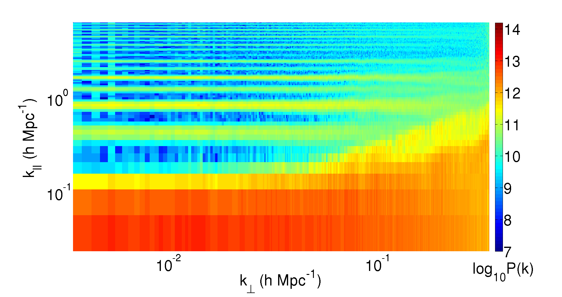
Figure 10.— The results of the simulation of noise and foregrounds are shown. The power spectrum pipeline developed to analyse the data is also applied to simulated foregrounds and noise for a three hour observational run for a single polarization.

Appendix B Appendix B: power spectrum estimation

As discussed in Section 4.1, the power spectrum from the data is computed in two stages. First the power spectrum and its RMS is computed for a single cell in which the HI signal is expected to be near coherent and then an average is obtained across cells assuming the HI signal to be incoherent for different cells (Figure 7).

As noted in the text, the HI signal can be recovered from a visibility cross-correlation by inverse weighing with ${\cal W}$. We denote such a cross correlation: $\hat{S}\equiv VV/{\cal W}$; $\hat{S}$ is generally a complex number. For optimal averaging to get the lowest noise estimator, one needs to sum over these cross-correlations by inverse weighing with the square of the RMS of each cross-correlation $\sigma_{i}$. For pure noise, $\sigma_{i}\propto 1/{\cal W}$ and one can obtain Eq. (32). Notice that this estimator is invariant under an overall scaling of $\sigma_{i}$. The error on power spectrum for each cell $\sigma_{p}$ is: $\sigma_{p}^{2}=\langle\hat{S}^{2}\rangle-\langle\hat{S}\rangle^{2}$, where the average is obtained optimally from the data for all the cross-correlations. It can be shown that if each cross-correlation is assumed to be uncorrelated, as would be the case for pure noise, $\sigma_{p}\simeq(1/\sum\sigma_{i}^{2})^{-1/2}$. Notice that if the RMS for all the cross-correlations is the same, as would be the case if all measurements are equally weighted, then this expression reduces to $\sigma_{p}=\sigma_{i}/\sqrt{N_{c}}$, where $N_{c}$ is the number of all the cross-correlations within a cell.

This procedure yields an estimate of the power spectrum (Eq. (32)) and its error $\sigma_{p}$ for each cell.

For averaging over cells, we repeat the procedure described above by taking the estimated power spectrum for a cell as the signal and $\sigma_{p}$ as the weights. This allows us to estimate 2- and 1-dimensional power spectrum and its RMS. For pure noise, the final error on the power spectrum is expected to approach: $\sigma_{\rm fin}=\sigma_{p}/\sqrt{N}$, where $N$ is the number of cells used for obtaining the average.

We briefly discuss some shortfalls of such a procedure. First, we do not construct the covariance matrix of the power spectrum estimator. We only estimate its diagonal terms, $\sigma_{p}^{2}$ and $\sigma_{\rm fin}^{2}$. This means that we are not able to assess the extent of cross-correlation between two neighbouring bins in Figure 9. Such cross-correlation might contain important information about systematic errors, foreground leakage, and HI signal and noise cross correlation.

Second, we do not include the HI signal in our estimation procedure. This is justified for the present work as the observed signal is clearly dominated by noise and foreground residuals (Figure 9). We briefly assess the impact of the HI signal for computing the error on the power spectrum.

We assume the following estimator for computing the power spectrum for a cell and consider the contribution of only the HI signal:

$$\hat{S}={1\over N_{c}}\sum_{ij}{V_{i}V_{j}\over{\cal W}_{ij}}$$ (B1)

As noted above, this estimator allows us to recover the HI signal. The subscripts $ij$ correspond to a pair for visibilities and the sum is carried over all the cross-correlations. After further computation, we obtain the error on the signal:

$$\Delta\hat{S}^{2}={\hat{S}^{2}\over N_{c}^{2}}\sum_{kl}\sum_{ij}\left[{{\cal W}_{ik}{\cal W}_{jl}+{\cal W}_{il}{\cal W}_{jk}\over{\cal W}_{ij}{\cal W}_{kl}}\right]$$ (B2)

If all the weights are unity this reduces to the usual cosmic variance expression: $\Delta\hat{S}=\sqrt{2}\hat{S}$. Even though this term is negligible for our purposes, this would need to be included for longer integration times.

References

- Ali et al. (2008) Ali, S. S., Bharadwaj, S., & Chengalur, J. N. 2008, MNRAS, 385, 2166
- Ali et al. (2015) Ali, Z. S. et al., 2015, ApJ, 809, 61
- Barkana & Loeb (2001) Barkana, R., Loeb, A., 2001, Phys.Rep., 349, 125-238
- Beardsley et al. (2013) Beardsley et al., 2013, MNRAS, 429, L5-L9
- Bharadwaj & Ali (2005) Bharadwaj S., Ali S. S., 2005, MNRAS, 356, 1519
- Bharadwaj & Sethi (2001) Bharadwaj, S., Sethi, S. K., 2001, JApA, 22, 293-307
- Bowman et al. (2009) Bowman, J. D. and Morales, M. F. and Hewitt, J. N., 2009, ApJ, 695, 183-199
- Bowman et al. (2013) Bowman, J. D., Cairns, I., Kaplan, D. L., et al. 2013, PASA, 30, 31
- Chapman et al. (2012) Chapman, E., et al. 2012, MNRAS, 423, 2518
- Chapman et al. (2013) Chapman, E., et al. 2013, MNRAS, 429, 165
- Christiansen & Hogbom (1969) Christiansen, W. N., & Hogbom, J. A. 1969, Radiotelescopes (Cambridge: Cambridge Univ. Press)
- Datta et al. (2010) Datta, A., Bowman, J. D., & Carilli, C. L. 2010, ApJ, 724, 526
- Datta et al. (2007) Datta K. K., Roy Choudhury T., Bharadwaj S., 2007, MNRAS, 378, 119
- Dillon et al. (2013) Dillon, J., Liu, A., & Tegmark, M. 2013, Phys. Rev. D, 87, 43005
- Dillon et al. (2014) Dillon, J. S., Liu, A., Williams, C. L., et al. 2014, Phys. Rev. D, 89, 023002
- Dillon et al. (2015) Dillon, J. S. et al. 2015, Phys. Rev. D, 91, 123011
- Fan et al. (2000) Fan, X., Carilli, C.L., & Keating, B., 2006, ARA&A, 44, 415
- Schwab (1984) F. R. Schwab., 1984, AJ, 89:1076–1081
- Furlanetto et al. (2006) Furlanetto, S. R., Oh, S. P., & Briggs, F. H. 2006, Phys.Rep., 433, 181-301
- Harker et al. (2009) Harker, G. et al. 2009, MNRAS, 397, 1138
- Haslam et al. (1982) Haslam, C. G. T., Stoffel, H., Salter, C. J., & Wilson, W. E. 1982, A&AS, 47, 1
- Hazelton et al. (2013) Hazelton, B. J., Morales, M. F., Sullivan, I. S., 2013, ApJ, 770, 156
- Hazelton et al. (2016) Hazelton, B. J., et al. 2016, in prep
- Hobson et al. (1995) Hobson M. P., Lasenby A. N., Jones M., 1995, MNRAS, 275, 863
- Hopkins et al. (2003) Hopkins, A. M., Afonso, J., Chan, B., et al. 2003, AJ, 125, 465
- Jacobs et al. (2016) Jacobs, D. C., et al. 2016, submitted in ApJ
- Jelic et al. (2008) Jelic, V. et al., 2008, MNRAS, 389, 1319
- Komatsu et al. (2010) Komatsu, E., et al. 2010, arxiv:1001.4538
- Liu et al. (2014a) Liu, Adrian., Parsons, Aaron R., Trott, Cathryn M., 2014a, Phys. Rev. D, 90, 023018
- Liu et al. (2014b) Liu, Adrian., Parsons, Aaron R., Trott, Cathryn M., 2014b, Phys. Rev. D, 90, 023019
- Liu & Tegmark (2011) Liu, A. & Tegmark, M., 2011, Phys. Rev. D, 83, 103006
- Lonsdale et al. (2009) Lonsdale, C. J., Cappallo, R. J., Morales, M. F., et al. 2009, IEEE Proceedings, 97, 1497
- McMullin et al. (2007) McMullin, J. P., Waters, B., Schiebel, D., Young, W., & Golap, K. 2007, Astronomical Data Analysis Software and Systems XVI (ASP Conf. Ser. 376), ed. R. A. Shaw, F. Hill, & D. J. Bell (San Francisco, CA: ASP), 127
- McQuinn et al. (2006) McQuinn, M., Zahn, O., Zaldarriaga, M., Hernquist, L., & Furlanetto, S. R., 2006, ApJ, 653, 815
- Mitchell et al. (2008) Mitchell, D. A., Greenhill, L. J., Wayth, R. B., Sault, R. J., Lonsdale, C. J., Cappallo, R. J., Morales, M. F., & Ord, S. M., 2008, IEEE Journal of Selected Topics in Signal Processing, 2, 707
- Morales & Hewitt (2004) Morales, M. F. & Hewitt, J. 2004, ApJ, 615,7
- Morales (2005) Morales, M. F., 2005, ApJ, 619, 678
- Morales & Wyithe (2010) Morales, M. F., & Wyithe, J. S. B. 2010, ARA&A, 48, 127
- Morales et al. (2012) Morales, M. F., Hazelton, B., Sullivan, I., & Beardsley, A. 2012, ApJ, 752, 137
- Nuttall (1981) Nuttall, A. H., 1981, IEEE Transactions on Acoustics Speech and Signal Processing, 29, 84
- Offringa et al. (2015) Offringa, A. R. et al, 2015, PASA, 32, 8
- Ord et al. (2010) Ord, S. M. et al. 2010, Publications of the Astronomical Society of the Pacific, 122, 1353
- Paciga et al. (2013) Paciga, G., et al. 2013, MNRAS, 433, 639
- Parsons et al. (2009) Parsons, A. R., & Backer, D. C. 2009, AJ, 138, 219
- Parsons et al. (2012a) Parsons, A., Pober, J. et al., 2012a, ApJ, 753, 81
- Parsons et al. (2012b) Parsons, A. R., Pober, J. C. et al., 2012b, ApJ, 756, 165p
- Parsons et al. (2014) Parsons, A. R., et al. 2014, ApJ, 788, 106
- Paul & Sethi et al. (2014) Paul, S., Sethi, S. K. et al., 2014, ApJ, 793, 28
- Pen et al. (2009) Pen, U. L., Chang, T. C., Hirata, C. M., Peterson, J. B., Roy, J., Gupta, Y., Odegova, J., Sigurdson, K., 2009, MNRAS, 399, 181
- Planck 2015 results. XIII. (2015) Planck Collaboration and Ade, P. A. R. and Aghanim, N. and Arnaud, M. and Ashdown, M. and Aumont, J. and Baccigalupi, C. and Banday, A. J. and Barreiro, R. B. and Bartlett, J. G. and et al., 2015, arXiv:1502.01589
- Planck 2016 results. XLVII. (2016) Planck Collaboration and Ade, R. and Aghanim, N. et al., 2016, arXiv:1605.03507v2
- Planck 2013 results. XVI. (2013) Planck Collaboration and Ade, P. A. R. and Aghanim, N. et al. 2013, Planck 2013 Results. XVI. Cosmological Parameters, arXiv:1303.5076
- Pober et al. (2013) Pober, J. C., Parsons, A. R. et al., 2013, ApJ, 768L, 36
- Presley et al. (2015) Presley, M.E., Liu, A., Parsons, A.R., 2015, ApJ, 809, 18
- Rau & Cornwell (2011) Rau, U. and Cornwell, T. J., 2011, Astronomy & Astrophysics, 532, A71
- Singh et al. (2015) Singh, S., Subrahmanyan, R., Udaya Shankar, N., Raghunathan, A., 2015, ApJ, 815, 88
- Sullivan et al. (2012) Sullivan, I. S. et al. 2012, The Astrophysical Journal, 759, 17
- Perley (1999) Taylor, G. B., Carilli, C. L., & Perley, R. A. 1999, Synthesis Imaging in Radio Astronomy II, 180, Chapter 19
- Thyagarajan et al. (2013) Thyagarajan, N., Udaya Shankar, N., Subrahmanyan, R., et al., 2013, ApJ, 776, 6
- Thyagarajan et al. (2015a) Thyagarajan, N. et al., 2015a, ApJ, 804, 14
- Thyagarajan et al. (2015b) Thyagarajan, N. et al., 2015b, The Astrophysical Journal Letters, 807, L28
- Thyagarajan et al. (2016) Thyagarajan, N., Parsons, A., DeBoer, D., et al., 2016, ArXiv e-prints, arXiv:1603.08958
- Tingay et al. (2013) Tingay, S. J. et al., 2013, PASA, 30.
- Cornwell et al. (2008) T. J. Cornwell, K. Golap, and S. Bhatnagar, 2008, IEEE Journal of Selected Topics in Signal Processing, 2:647–657
- Trott et al. (2012) Trott, C., Wayth, R., & Tingay, S. 2012, ApJ, 757, 101
- Trott et al. (2016) Trott, C. M. et al., 2016, ApJ, 818, 139
- Van Haarlem et al. (2013) Van Haarlem, M. P. et al. Astron. Astrophys. 556, A2 (2013)
- Vedantham et al. (2012) Vedantham, H., Udaya Shankar, N., & Subrahmanyan, R. 2012, ApJ, 745, 176
- Zaldarriaga et al. (2004) Zaldarriaga, M., Furlanetto, S. R., & Hernquist, L., 2004, ApJ, 608, 622
- Zaroubi (2013) Zaroubi, Saleem, 2013, Astrophysics and Space Science Library, 396, arxiv: 1206.0267
- Zheng et al. (2016) Zheng, Q., Wu, X.-P., Hollitt, M. J., Gu, J.-H., Xu, H., 2016, arXiv:1602.06624v1