Lick Indices and Spectral Energy Distribution Analysis based on an M31 Star Cluster Sample: Comparisons of Methods and Models

Abstract

Application of fitting techniques to obtain physical parameters—such as ages, metallicities, and $\alpha$-element to iron ratios—of stellar populations is an important approach to understand the nature of both galaxies and globular clusters (GCs). In fact, fitting methods based on different underlying models may yield different results, and with varying precision. In this paper, we have selected 22 confirmed M31 GCs for which we do not have access to previously known spectroscopic metallicities. Most are located at approximately one degree (in projection) from the galactic center. We performed spectroscopic observations with the 6.5 m MMT telescope, equipped with its Red Channel Spectrograph. Lick/IDS absorption-line indices, radial velocities, ages, and metallicities were derived based on the $\rm EZ\_Ages$ stellar population parameter calculator. We also applied full spectral fitting with the ULySS code to constrain the parameters of our sample star clusters. In addition, we performed $\chi^{2}_{\rm min}$ fitting of the clusters’ Lick/IDS indices with different models, including the Bruzual & Charlot models (adopting Chabrier or Salpeter stellar initial mass functions and 1994 or 2000 Padova stellar evolutionary tracks), the galev, and the Thomas et al. models. For comparison, we collected their $UVBRIJK$ photometry from the Revised Bologna Catalogue (v.5) to obtain and fit the GCs’ spectral energy distributions (SEDs). Finally, we performed fits using a combination of Lick/IDS indices and SEDs. The latter results are more reliable and the associated error bars become significantly smaller than those resulting from either our Lick/IDS indices-only or our SED-only fits.

1 Introduction

Globular clusters (GCs) are good tracers to aid in our understanding of the formation, evolution, and interactions of galaxies. Since most GCs were formed during the early stages of their host galaxies’ life cycles, they are often considered the fossils of the galaxy formation and evolution processes (Barmby et al., 2000). Since GCs are dense and luminous, so that they can be detected at great distances, they could be useful probes for studying the properties of distant extragalactic systems. Since halo globular clusters (HGCs) are located at great distances from their host galaxies’ centers, they are useful to study the dark matter distributions in their host galaxies. Another advantage of observing HGCs is the reduced galaxy background contribution, enabling us to achieve sufficiently high signal-to-noise ratios (SNR) fairly easily.

The Pan-Andromeda Archaeological Survey (PAndAS; McConnachie et al., 2009) has obtained observations of the nearby galaxies Messier 31 (M31, the Andromeda galaxy) and its companion galaxy, Messier 33 (M33), with the MegaPrime/MegaCam camera at the 3.6 m Canada-–France-–Hawai’i Telescope (CFHT). The survey reaches depths of $g=26.5$ mag and $i=25.5$ mag, which has enabled discoveries of a great number of substructures and giant stellar streams in the M31/M33 halo. These structures are faint and spatially extended, thus making them difficult to observe using either imaging or spectroscopy. However, the system’s HGCs may be good tracers of these structures (if they are at least spatially related to the stellar streams), since the HGCs are bright and characterized by centrally concentrated luminosity profiles. They can hence be used to study the interaction between M31 and M33.

The number of M31 GCs is estimated to range from $460\pm 70$ (Barmby & Huchra, 2001) to $\sim$530 (Perina et al., 2010), including dozens of HGCs. Huxor et al. (2004) discovered nine previously unknown M31 HGCs based on the Isaac Newton Telescope (INT) survey. Subsequently, Huxor et al. (2005) discovered three new extended GCs in the halo of M31, whose nature appears to straddle the parameter space between typical GCs and dwarf galaxies. Mackey et al. (2006) reported four extended, low surface brightness star clusters in the halo of M31 based on Hubble Space Telescope (HST)/Advanced Camera for Surveys (ACS) imaging. Huxor (2007) found 40 new, extended GCs in the halo of M31 at $\sim 100$ kpc from the galactic center, based on the INT and CFHT imaging surveys. Recently, Fan et al. (2011, 2012) observed dozens of confirmed M31 HGCs using the OptoMechanics Research, Inc. (OMR) spectrograph on the 2.16 m telescope (see, Fan et al., 2016) at Xinglong Observatory (National Astronomical Observatories, Chinese Academy of Sciences) in the Fall seasons of 2010 and 2011. They estimated the ages, metallicities, and $\alpha$-element abundances using simple stellar population (SSP) models, as well as radial velocities, $V_{r}$. They found that most HGCs are old and metal-poor. Evidence of a metallicity gradient was also uncovered, although at a low level of significance.

Stellar population fitting techniques are important tools to constrain the physical parameters—e.g., the ages, metallicities, and $\alpha$-element abundances—of GCs; $\chi^{2}_{\rm min}$ fitting of GC spectral energy distributions (SEDs) is an efficient way to derive these parameters on the basis of photometry (see, e.g., Fan et al., 2006, 2010; Fan & de Grijs, 2012, 2014; Ma et al., 2007, 2009, 2010, 2011; Wang et al., 2010), while spectroscopic fitting is an alternative, equally efficient approach to deriving these parameters. In fact, many different spectroscopic fitting techniques have been developed. One of these involves full spectral fitting, e.g., using ULySS (Koleva et al., 2009; Chen et al., 2016). Alternatively, one could pursue $\chi^{2}_{\rm min}$ fitting of various Lick/IDS indices (e.g., Fan et al., 2011, 2012; Chen et al., 2016). Each method is associated with its own advantages and disadvantages. Of course, the results and precision are model-dependent. Availability of more and more useful information obviously leads to higher precision, all else being equal. Therefore, $\chi^{2}_{\rm min}$ fitting combined with SED and Lick-index fitting is expected to provide more reliable and higher-precision results than any of these approaches on their own.

In this paper, we compare the results of different fitting methods to the observables of 22 M31 HGCs using SED-only and Lick-index-only data, and their combination. This paper is organized as follows. In Section 2 we describe our sample of M31 GCs and their spatial distribution. In Section 3 we provide an overview of our spectroscopic observations with the 6.5 m MMT telescope and the data reduction, including our measurements of the radial velocities and Lick indices. Subsequently, in Section 4, we derive and discuss the ages, metallicities, and $\alpha$-element abundances based on $\chi^{2}_{\rm min}$ fitting, using various models and methods. Finally, we summarize our work and offer our conclusions in Section 5.

2 GC Sample Selection

Our sample star clusters were mainly selected from Peacock et al. (2010), who provide a catalog of 416 old, 156 young, and 373 candidate clusters. This catalog is based on $ugriz$ and $K$-band photometry using observations with the Wide Field Camera (WFCAM) mounted on the United Kingdom Infrared Telescope (UKIRT) and the Sloan Digital Sky Survey (sdss). We selected those confirmed star clusters from Peacock et al. (2010) without previously determined spectroscopic metallicities. Fan et al. (2008) published a spectroscopic metallicity catalog (‘SMCat’) based on spectroscopic metallicities found in the literature, specifically in Perrett et al. (2002), Huchra et al. (1991), and Barmby et al. (2000). Their catalog contains 295 entries. In addition, we also include the complementary spectroscopic metallicities of Galleti et al. (2009), leading to a final database of 329 metallicities.

We next excluded star clusters with previous spectroscopic metallicity determinations. Thus, we obtained a catalog of 102 confirmed GCs which lack spectroscopic metallicities or radial velocities. In addition, since we are interested in halo star clusters and to achieve sufficiently high SNRs for the observations, we removed star clusters located inside a projected distance of $r_{\rm p}=1$ degree from the the galaxy’s center. Since the local background near the galaxy center is too luminous for our observations, we were left with only 35 GCs. Of these, we observed 17 randomly chosen objects given the limited observing time we had access to, thus minimizing selection effects. The magnitudes of our sample star clusters range from $V=15.5$ mag to $V=18.2$ mag. For comparison, we also included five star clusters (SK001A, B423, B298, B006, and B017) which have their radial velocities listed in the Revised Bologna Catalogue of M31 GCs and candidates (RBC v.4, Galleti et al., 2004, 2006, 2009). B423 is listed as a confirmed star cluster in the RBC v.4 but classified as a star cluster candidate in Peacock et al. (2010). It does not have any previously obtained spectroscopic information.

The observational information of our sample GCs is listed in Table 1, which includes the cluster identification (Col. 1), coordinates (R.A. and Dec. in Cols. 2 and 3, respectively), projected radii from the galaxy center, $r_{\rm p}$, in kpc (Col. 4), $V$-band magnitude (Col. 5), exposure time (Col. 6), and observation date(s) (Col. 7). In fact, the coordinates, $r_{\rm p}$, and $V$-band magnitudes were taken from the RBC v.5. The projected radii were calculated for the M31 center coordinates (J2000: 00:42:44.31, $+$41:16:09.4; Perrett et al., 2002), a position angle (PA) of $38^{\circ}$, and a distance $d=785$ kpc (McConnachie et al., 2005). SK001A is classified as a confirmed star cluster in the RBC v.4, but in the updated RBC v.5 it has been re-classified as a star. Since we performed our observations before the RBC v.5 was updated, SK001A was included in our observing campaign.

In Fig. 1 we show the spatial distribution of our sample star clusters. The large ellipse is the M31 disk/halo boundary as defined by Racine (1991); the two smaller ellipses trace out NGC 205 and M32. Note that most of our sample GCs are located in the projected direction of the M31 halo, which could help us to better understand the nature of the galaxy’s halo with the enlarged cluster sample of Fan et al. (2011, 2012).

3 Observations and Data Reduction

Spectroscopic observations were carried out with the 6.5 m MMT/Red Channel Spectrograph from 2010 October 31 to 2010 November 2 and on 2011 November 4. The telescope is located on Mt. Hopkins in Arizona (USA) at an altitude of 2581 m. The exposure times used ranged from 480 s to 1800 s, depending on the cluster brightness. The median seeing was $\sim 0^{\prime\prime}.98$ and we adopted a slit aperture of $0^{\prime\prime}.75\times 180^{\prime\prime}$. The CCD’s size is 450$\times$1032 pixels². It is characterized by a gain of 1.3 e^- ADU^-1, with a readout noise (RN) of 3.5 e^-. A grating with 600 $l$ mm^-1 with a blaze 1st/4800 was used. The spectral resolution was $R=960$ for slit of 1” and a central wavelength of 4701Å; the dispersion was 1.63Å pixel^-1.

The spectroscopic data were reduced following standard procedures with the NOAO Image Reduction and Analysis Facility (iraf v.2.15) software package. First, all spectral images were checked carefully. Next, we performed bias combination with zerocombine and bias correction with ccdproc. Subsequently, flat-field combination, normalization, and corrections were done using flatcombine, response, and ccdproc, respectively. Cosmic rays were removed using cosmicrays. We extracted both the star cluster spectra and those obtained from a comparison arc lamp with apall. Wavelength calibration was done with helium/argon-lamp spectra taken at both the beginning and the end of observations during each night. The spectral features of the comparison lamps were identified with identify and wavelength calibration was done with refspectra. We next used dispcor for dispersion correction and to resample the spectra. Flux calibration was performed based on observations of four Kitt Peak National Observatory (KPNO) spectral standard stars (Massey et al., 1988). We applied standard and sensfunc to combine the standards and to determine the sensitivity and extinction. Atmospheric extinction was corrected for using the mean extinction coefficients pertaining to KPNO. Finally, we applied calibrate to correct for the extinction and complete the flux calibration.

Figure 2 shows the normalized, calibrated spectra of our sample GCs, identified by their names. The signal-to-noise ratios of most GCs are high, except for those of a few faint clusters such as H16, H15, and B436.

4 Fitting, Analysis, and Results

4.1 Full-Spectrum Fitting with ULySS

ULySS (Koleva et al., 2009) was used for the full spectral fitting of the ages and metallicities. The Vazdekis et al. (2010) SSP models adopted are based on the miles (Medium-resolution INT Library of Empirical Spectra) spectral library (Sánchez-Blázquez et al., 2006). The wavelength coverage ranges from 3540.5Å to 7409.6Å at a nominal resolution full width at half maximum, FWHM = 2.3Å. The solar-scaled theoretical isochrones of Girardi (2000) were adopted and we used the stellar initial mass function (IMF) of Salpeter (1955) for the fitting. The age coverage was $10^{8}$–$1.5\times 10^{10}$ yr and the metallicity ranged from [Fe/H] = $-2.32$ dex ($Z=0.0004$) to [Fe/H] = $+0.22$ dex ($Z=0.03$). An independent SSP model set, pegase-hr, is provided by Le Borgne et al. (2004), which is based on the empirical spectral library elodie (e.g., Prugniel & Soubiran, 2001; Prugniel et al., 2007). The elodie wavelength coverage spans the range from 3900Å to 6800Å. The spectral resolution is $R\sim 10,000$ with a FWHM of $\sim 0.55$Å. The effective temperature, $T_{\rm eff}$, range is 3100–50,000 K, the gravity, $log~{}g$, ranges from $-0.25$ dex to 4.9 dex, and the metallicity $\rm[Fe/H]$ ranges from $-3$ dex to $+1$ dex. The flux calibration accuracy is 0.5–2.5% from narrow to broad bands. We adopted the pegase-hr SSP models with a Salpeter (1955) IMF. The model ages we adopted cover the range $10^{7}$–$1.5\times 10^{10}$ yr, and the metallicity ranges from [Fe/H] = $-2.0$ dex ($Z=0.0004$) to [Fe/H] = $+0.4$ dex ($Z=0.05$).

Figure 3 shows the observed MMT spectroscopy of the star cluster B006–G058 combined with the best-fitting model from pegase-hr. For the full spectral fitting we only consider the wavelength range $\sim 4000$–$5400$Å for SNR reasons. In the top panel, the observed spectrum is shown in black, the best-fitting spectrum from the pegase-hr models is rendered in blue, and the outliers are shown in red. The cyan lines delineate the multiplicative polynomials. The bottom panels are the fractional residuals of the best fits. The dashed and solid lines in green denote zero and the 1$\sigma$ deviations, respectively, which were calculated based on the variance of the input (observed) spectrum. For all sample star clusters, the results of the fits are good and the residuals are small.

The radial velocities and their associated uncertainties are fitted with ULySS based on both the Vazdekis et al. (2010) and pegase-hr SSP models. The results are included in Table 2. For comparison, we also list the $V_{r}$ values from the RBC v.5. For most GCs, the values resulting from the Vazdekis et al. (2010) and pegase-hr SSP models are rather similar. The median $V_{r}$ values are $-353$ km s^-1 for the Vazdekis et al. (2010) models and $-351$ km s^-1 for the pegase-hr SSP models. Both yield a velocity difference of $\sim-50$ km s^-1 relative to the systematic velocity of M31, $\sim-300$ km s^-1. Note that for most clusters, the $V_{r}$ values derived from our ULySS fits are consistent with those from the RBC v.5, except for a few clusters (G339–BA30, G260, and SK001A). We carefully checked the spectroscopy and concluded that the fit results are reasonable and stable. The RBC v.5 data were collected from various sources in the literature, some of which may have large measurement uncertainties but which are not listed in the RBC v.5. The systematic differences between the observed velocities and the catalog velocity are $-63\pm 137$ km s^-1 for the Vazdekis et al. (2010) models and $-61\pm 147$ km s^-1 for the pegase-hr models. This indicates that our measurements agree well with those in the RBC v.5, since the systematic differences between our measurements and the published values are not significant. For some star clusters, the differences between our measurements and the published values are relatively large, which may be due to the different kinds or numbers of spectral features or methods used for the measurements and analysis.

Table Lick Indices and Spectral Energy Distribution Analysis based on an M31 Star Cluster Sample: Comparisons of Methods and Models summarizes the resulting logarithmic ages and the metallicities derived based on the Lick absorption-line indices and fitted with ULySS, for both the Vazdekis et al. (2010) and pegase-hr SSP models. As expected, the ages and metallicities resulting from both model sets are essentially the same. All our sample GCs are old and metal-poor: for the Vazdekis et al. (2010) SSP models, $\rm age_{mean}=11.7$ Gyr (with an r.m.s. spread of $3.9$ Gyr) and $\rm[Fe/H]_{mean}=-1.37$ dex (r.m.s. = $0.60$ dex); for the pegase-hr models, $\rm age_{mean}=12.9$ Gyr (r.m.s. = $6.4$ Gyr) and $\rm[Fe/H]_{mean}=-1.41$ dex (r.m.s. = $0.62$ dex), which is consistent with previous results.

Figure 4 displays the relationship between the metallicities and the ages of our sample GCs fitted with ULySS (from Table Lick Indices and Spectral Energy Distribution Analysis based on an M31 Star Cluster Sample: Comparisons of Methods and Models). The associated error bars are also shown; they are relatively small. The left- and right-hand panels show the parameters resulting from the Vazdekis et al. (2010) and the pegase-hr SSP models, respectively. The results are rather similar. All star clusters are old and most are metal-poor, since most of the sample clusters are located in the halo of the galaxy.

4.2 Lick-Index Fitting with $\rm EZ\_Ages$

$\rm EZ\_Ages$ is an automated stellar population analysis tool written in idl. The code is used to compute the mean light-weighted ages, metallicities [Fe/H], and the elemental abundances [Mg/Fe], [C/Fe], [N/Fe], and [Ca/Fe] from integrated spectra for various unresolved stellar populations (Graves & Schiavon, 2008). Recently, Chen et al. (2016) successfully tested the $\rm EZ\_Ages$ package by fitting Large Sky Area Multi-Object Fibre Spectroscopic Telescope (LAMOST) spectroscopy of Galactic GCs with known ages and chemical compositions, which they subsequently applied to a sample of M31 star clusters.

We applied the $\rm EZ\_Ages$ code to estimate the Lick indices as well as the ages and abundances of our sample GCs. Before measuring the Lick indices, the resolution was adjusted with a variable-width Gaussian kernel following the definition of Worthey & Ottaviani (1997), i.e., 11.5Å at 4000Å, 9.2Å at 4400Å, 8.4Å at 4900Å, 8.4Å at 5400Å, and 9.8Å at 6000Å. Since the wavelength coverage of the MMT’s Red Channel Spectrograph is $\sim 3900$–$5500$Å, we measured all 20 Lick indices defined in this regime. The measurements were strictly done following Worthey et al. (1994a) and Worthey & Ottaviani (1997). The uncertainty in each index was estimated following Cardiel et al. (1998, their Eqs 11–18).

Table Lick Indices and Spectral Energy Distribution Analysis based on an M31 Star Cluster Sample: Comparisons of Methods and Models lists the ages and metallicities derived with $\rm EZ\_Ages$. Note that many GCs do not have age or metallicity values owing to fitting failures of the $\rm EZ\_Ages$ code. Since $\rm EZ\_Ages$ does not perform model extrapolation, stellar populations with line index measurements outside the model grid are excluded from the analysis. This applies to models with metallicities $\rm[Fe/H]<-1.3$ dex or $\rm[Fe/H]>+0.2$ dex. The metallicities $\rm[Fe/H]_{[MgFe]}$ are also given in Table Lick Indices and Spectral Energy Distribution Analysis based on an M31 Star Cluster Sample: Comparisons of Methods and Models; they were derived from $\rm[MgFe]$; $\rm[MgFe]=\rm\sqrt{Mg{\it b}\times\langle Fe\rangle}$, where $\rm\langle Fe\rangle=(Fe5270+Fe5335)/2$. Thus, the metallicity can be calculated following Galleti et al. (2009), using

$$\rm[Fe/H]_{[MgFe]}=-2.563+1.119[MgFe]-0.106[MgFe]^{2}\pm 0.15dex(r.m.s.).$$ (1)

Similarly, the metallicities $\rm[Fe/H]_{\langle Fe\rangle}$, derived from $\rm\langle Fe\rangle=(Fe5270+Fe5335)/2$ following Caldwell et al. (2011), are also listed in Table Lick Indices and Spectral Energy Distribution Analysis based on an M31 Star Cluster Sample: Comparisons of Methods and Models.

4.3 Lick Index Fitting with Stellar Population Models

Thomas et al. (2003) provided stellar population models which included Lick absorption-line indices for various elemental-abundance ratios. The model suite’s age coverage ranges from 1 Gyr to 15 Gyr and the metallicities span from 1/200 to 3.5 times solar abundance. These models are based on the standard models of Maraston (1998) and the input stellar evolutionary tracks are from Cassisi et al. (1997) and Bono et al. (1997). The Salpeter (1955) stellar IMF was adopted. Subsequently, Thomas et al. (2004) improved the models by including higher-order Balmer absorption-line indices and found that these indices are sensitive to changes in the $\rm\alpha/Fe$ ratio for supersolar metallicities. The updated stellar population models for Lick absorption-line indices of Thomas et al. (2011) represent an improvement with respect to Thomas et al. (2003) and Thomas et al. (2004); they are based on the miles stellar library (Sánchez-Blázquez et al., 2006). The model provides a higher spectral resolution appropriate for miles and sdss spectroscopy with calibrated fluxes. The models cover ages from 0.1 Gyr to 15 Gyr (0.1, 0.2, 0.4, 0.6, 0.8, 1, 2, 3, 4, 5, 6, 7, 8, 9, 10, 11, 12, 13, 14, and 15 Gyr), the metallicity ranges from $\rm[Z/H]=-2.25$ dex to 0.67 dex ($-2.25$, $-1.35$, $-0.33$, 0.0, 0.35, and 0.67 dex), and the $\alpha$-element ratio $\rm[\alpha/Fe]$ spans from $-0.3$ dex to 0.5 dex ($-0.3$, 0.0, 0.3, and 0.5 dex). The models are based on the evolutionary synthesis code of Maraston (2005). The stellar evolutionary tracks adopted come from Cassisi et al. (1997) and Girardi (2000) (i.e., the Padova models), especially for $\rm[Z/H]=0.67$ dex. We fitted the absorption-line indices with the models of Thomas et al. (2011), adopting the stellar evolutionary tracks of Cassisi et al. (1997). In fact, the models were interpolated to allow for smaller parameter intervals to improve the resolution of the parameters. Cubic spline interpolations were adopted, using equal step lengths, to obtain a grid of 150 ages (from 0.1 Gyr to 15 Gyr), 31 $\rm[Z/H]$ values (from $-2.25$ dex to 0.67 dex), and 31 $\rm[\alpha/Fe]$ ratios (from $-0.3$ dex to $0.5$ dex), which results in fits that are smoother and more continuous.

As mentioned in Section 4.2, because of the limited wavelength coverage of our sample GCs, we only measured 20 Lick absorption-line indices. Since the Lick indices are not sensitive to reddening, as opposed to our SED fits, we did not consider the reddening in our Lick-index fitting. Similarly to Fan et al. (2011, 2012), the ages $t$, metallicities $\rm[Z/H]$, and the $\rm[\alpha/Fe]$ ratios can be determined by comparing the interpolated stellar population models with observational spectral indices by employing the $\chi^{2}$-minimization method,

$$\chi^{2}_{\rm min}={\rm min}\left[\sum_{i=1}^{20}\left({\frac{L_{\lambda_{i}}^{\rm obs}-L_{\lambda_{i}}^{\rm mod}(t,\rm[Z/H],[\alpha/Fe])}{\sigma_{L,i}}}\right)^{2}\right],$$ (2)

where $L_{\lambda_{i}}^{\rm mod}(t,\rm[Z/H],[\alpha/Fe])$ is the $i^{\rm th}$ Lick absorption-line index in the stellar population model for $t$, $\rm[Z/H]$, and $\rm[\alpha/Fe]$; $L_{\lambda_{i}}^{\rm obs}$ represent the observed, calibrated Lick absorption-line indices from our measurements and the errors estimated from our fits are

$$\sigma_{L,i}^{2}=\sigma_{{\rm obs},L,i}^{2}+\sigma_{{\rm mod},L,i}^{2}.$$ (3)

Here, $\sigma_{{\rm obs},i}$ is the observational uncertainty; $\sigma_{{\rm mod},i}$ is the uncertainty associated with the model Lick indices, provided by Thomas et al. (2011) and Table 5 of Bruzual & Charlot (2003).

Table Lick Indices and Spectral Energy Distribution Analysis based on an M31 Star Cluster Sample: Comparisons of Methods and Models includes the resulting ages, metallicities, and $\rm[\alpha/Fe]$ ratios for the evolutionary tracks of Cassisi et al. (1997) and the Padova models of Thomas et al. (2011). Figure 5 shows the relationship between the ages and metallicities derived from the Thomas et al. (2011) models, which are also included in Table Lick Indices and Spectral Energy Distribution Analysis based on an M31 Star Cluster Sample: Comparisons of Methods and Models. Most GCs are older than or approximately 10 Gyr, and most metallicities are lower than $\rm[Z/H]=-1$ dex. This implies that our sample GCs are old and metal-poor, which is in agreement with the previous results we obtained using $\rm EZ\_Ages$, included in Table Lick Indices and Spectral Energy Distribution Analysis based on an M31 Star Cluster Sample: Comparisons of Methods and Models. Thus, this indicates that these HGCs formed during the early stages of galaxy formation, which agrees well with previous conclusions.

The Galaxy Evolutionary Synthesis Models (galev; Lilly & Fritze-v. Alvensleben, 2006; Kotulla et al., 2009) are evolutionary synthesis models that can be used to simultaneously explore both the chemical evolution of the gas and the spectral evolution of the stellar content in star clusters or galaxies. The models provide photometry and Lick absorption-line indices for different types of galaxies (i.e., different star-formation rates) or SSPs (single burst). The models provide 5001 ages from 4 Myr to 20 Gyr, and seven metallicities ($Z=0.0001$, 0.0004, 0.001, 0.004, 0.008, 0.02, and 0.05). As done previously, we interpolate the metallicities to a grid of 51 values which can yield more accurate results than the basic model set. The uncertainties in the Lick indices for the models in Eq. (3) are estimated using Equation (3) of Lilly & Fritze-v. Alvensleben (2006), while the observed uncertainties come from the estimated $\rm EZ\_Ages$ fits to the observations. The fit results are shown in Table Lick Indices and Spectral Energy Distribution Analysis based on an M31 Star Cluster Sample: Comparisons of Methods and Models and the age–metallicity distribution is shown in Fig. 6. Although more than half of the star clusters are older than 1 Gyr, there are still numbers of star clusters that are younger than 1 Gyr but associated with large uncertainties. This is different from our results based on Thomas et al. (2011). In fact, Fan & de Grijs (2012) already pointed out that the galev models are mainly suitable for young stellar populations; they usually produce younger ages than other models.

The evolutionary stellar population synthesis models of Bruzual & Charlot (2003, hereafter BC03) do not only provide spectra and SEDs for different physical parameters, but also Lick/IDS absorption-line indices. The models include the 1994 and 2000 Padova stellar evolutionary tracks as well as the Salpeter (1955) and Chabrier (2003) IMFs. The wavelength coverage ranges from 91Å to 160 $\mu$m. For the Padova 1994 tracks, models for six metallicities ($Z=0.0001$, 0.0004, 0.004, 0.008, 0.02, and 0.05) are provided, while for the Padova 2000 tracks, models of six different metallicities ($Z=0.0004$, 0.001, 0.004, 0.008, 0.019, and 0.03) are given. In total, there are 221 ages from 0 to 20 Gyr in unequally spaced time steps. Here we also interpolate the models to attain smaller intervals of the parameter space (51 metallicities with equal steps in logarithmic space) to obtain more accurate results. Similar to the fits based on the Thomas et al. (2011) models, Eqs (2) and (3) were adopted. In fact, we tried different combinations of Padova 1994/2000 stellar evolutionary tracks and IMFs. The results are given in Table Lick Indices and Spectral Energy Distribution Analysis based on an M31 Star Cluster Sample: Comparisons of Methods and Models and the relevant plots are shown in Fig. 7. It is clear that for the same stellar evolutionary tracks adoption of a different IMF does not affect the results (including the uncertainties) significantly. Note that the best-fitting metallicity range for the Padova 2000 tracks is not as wide as that obtained from the Padova 1994 tracks because of the models’ limitations.

4.4 Combination with SEDs and Comparisons with the BC03 models

We also acquired the clusters’ $UBVRIJHK$ photometry from the RBC v.5 and performed SED fitting to the sample GCs. Reddening affects the SED results more significantly than for the Lick/IDS indices. The reddening values for our sample star clusters were adopted from Fan et al. (2008) where available. If they were not available, we used $E(B-V)=0.1$ mag (e.g., van den Bergh, 1969; Frogel et al., 1980) instead, a representative value of the Galactic foreground reddening in the direction of M31. The extinction $A_{\lambda}$ can be computed using the equations of Cardelli et al. (1989), and we adopted a typical foreground Milky Way extinction law, $R_{V}=3.1$. We fitted the SEDs using

$$\chi^{2}_{\rm min}={\rm min}\left[\sum_{j=1}^{8}\left({\frac{M_{\lambda_{j}}^{\rm obs}-M_{\lambda_{j}}^{\rm mod}(t,\rm[Z/H],[\alpha/Fe])}{\sigma_{M,j}}}\right)^{2}\right],$$ (4)

where $M_{\lambda_{j}}^{\rm mod}(t,\rm[Z/H],[\alpha/Fe])$ is the $j^{\rm th}$ magnitude provided in the stellar population model for age $t$, metallicity $\rm[Z/H]$, and $\rm[\alpha/Fe]$; $M_{\lambda_{i}}^{\rm obs}$ represents the observed dereddened magnitude in the $j^{\rm th}$ band.

Similar to Eq. 3, Eq. 5 represents the errors associated with our fits,

$$\sigma_{M,j}^{2}=\sigma_{{\rm obs},M,j}^{2}+\sigma_{{\rm mod},M,j}^{2},$$ (5)

where $\sigma_{M,j}$ is the magnitude uncertainty in the $j^{\rm th}$ filter. We estimated the photometric errors in the RBC v.5 magnitudes. We adopted 0.08 mag in $U$, 0.05 mag in $BVRI$, 0.1 mag in $J$, and 0.2 mag in $HK$ (Galleti et al., 2004). The model errors adopted were 0.05 mag, which is the typical photometric error for the BC03 and galev SSP models (e.g., Fan et al., 2006; Ma et al., 2007, 2009; Wang et al., 2010; Fan & de Grijs, 2014).

The results of our SED fits are included in Table Lick Indices and Spectral Energy Distribution Analysis based on an M31 Star Cluster Sample: Comparisons of Methods and Models and the relevant plots are shown in Fig. 8. Similarly to Fig. 7, we tried different combinations of the Padova 1994/2000 stellar evolutionary tracks and IMFs. It is clear that for the same stellar evolutionary tracks, adoption of a different IMF does not affect the results (including the uncertainties) significantly. We found that the best-fitting ages are old for all clusters and the scatter in the parameter distribution is smaller than that resulting from the Lick absorption-line index fitting in Fig. 7.

The mathematical approach to simultaneously minimize the Lick absorption-line indices and SEDs with respect to the stellar population models is given by

$$\chi^{2}_{\rm min}={\rm min}\left[\sum_{i=1}^{20}\left({\frac{L_{\lambda_{i}}^{\rm obs}-L_{\lambda_{i}}^{\rm mod}(t,\rm[Z/H],[\alpha/Fe])}{\sigma_{L,i}}}\right)^{2}+\sum_{j=1}^{8}\left({\frac{M_{\lambda_{j}}^{\rm\ obs}-M_{\lambda_{j}}^{\rm mod}(t,\rm[Z/H],[\alpha/Fe])}{\sigma_{M,j}}}\right)^{2}\right],$$ (6)

where $L_{\lambda_{i}}^{\rm mod}(t,\rm[Z/H],[\alpha/Fe])$ and $M_{\lambda_{j}}^{\rm mod}(t,\rm[Z/H],[\alpha/Fe])$ are the $i^{\rm th}$ Lick absorption-line indices and the $j^{\rm th}$ magnitudes in the relevant stellar population model for age $t$, metallicity $\rm[Z/H]$, and $\rm[\alpha/Fe]$, respectively; $L_{\lambda_{i}}^{\rm obs}$ and $M_{\lambda_{j}}^{\rm obs}$ represent the observed, calibrated $i^{\rm th}$ Lick absorption-line indices and the observed, dereddened magnitude in the $j^{\rm th}$ band, respectively. The errors associated with the observations in our fits are given by Eqs (3) and (5).

In order to compare the results obtained from the different approaches, we also tried different combinations of Padova 1994/2000 stellar evolutionary tracks and IMFs. The final results are included in Table Lick Indices and Spectral Energy Distribution Analysis based on an M31 Star Cluster Sample: Comparisons of Methods and Models and a plot of the age–metallicity distribution is shown in Fig. 9. Note that the results seem better than those shown in Fig. 8, since the uncertainties in the parameters are significantly smaller than those resulting from the SED-only fitting method. They also look better than those from the Lick-indices-only fits in Fig. 7. It is clear that the uncertainties in the parameters and the scatter are much smaller. The HGCs are expected to be metal-poor and old, which is confirmed by the results of both our fits with ULySS and those based on the Thomas et al. (2011) models. Therefore, we conclude that combined fits of SEDs and Lick indices can significantly improve the reliability and accuracy of the results.

Figure 10 compares the ages resulting from the different models. For all panels, the $x$ axis is the age resulting from the combined fits of the Lick indices and SEDs, adopting the BC03 models, the Padova 1994 stellar evolutionary tracks, and a Chabrier (2003) IMF, a combination we use as our standard for comparison. Along the $y$ axis we display, at the top left, the results from the BC03 models, the Padova 1994 tracks, and Chabrier (2003) IMF fits of the Lick indices only. Fits based on only the Lick indices agree well with the combined fits, at least if we use the same models, the same tracks, and the same IMF, except for a few outliers.

At the top right, we show the results for the BC03 models, the Padova 1994 tracks, and Chabrier (2003)) IMF fits to the SEDs only. It is clear that the fits based on SEDs only agree well with the results from the combined fits for the same models, the same tracks, and the same IMF. The agreement is even better than that in the top left-hand panel. In the middle left-hand panel, we show the results from fits using the BC03 models, the Padova 2000 tracks, and a Chabrier (2003) IMF for the combination of SEDs and Lick indices. The models, methods, and IMFs used are exactly the same, except for our adoption of the Padova 1994/2000 evolutionary tracks, indicating that any differences between the two sets of evolutionary tracks are rather insignificant as regards the resulting ages. In the middle right-hand panel, we show the galev model fits to the Lick indices only. A few of the ‘old’ star clusters in the BC03 models are considered ‘young’ in the galev models, which is noted in Fig. 7 and explained in Fan & de Grijs (2012). At the bottom left, the results from Thomas et al. (2011) model fits to only the Lick indices are shown and at the bottom right we show the results from the ULySS models combined with Vazdekis et al. (2010) full-spectrum fits. Both the results from the Thomas et al. (2011) and those based on the ULySS fits using the Vazdekis et al. (2010) SSP models agree well with those from the BC03 models with the combined fits of the Lick indices and SEDs.

Figure 11 is the same as Fig. 10, but for the metallicity. The $x$ axis represents the metallicities obtained from fitting the combination of Lick indices and SEDs using the BC03 models, the Padova 1994 stellar evolutionary tracks, and a Chabrier (2003) IMF. As regards the $y$ axis, at the top left, we show the results of the BC03 models, the Padova 1994 tracks, and Chabrier (2003) IMF fits to only the Lick indices. The agreement is good, except for a few outliers. At the top right, results for the BC03 models, Padova 1994 tracks, and Chabrier (2003) fits to only the SEDs are shown. The agreement is not as good as that for the fits to only the Lick indices in the top left-hand panel. In the middle left-hand panel, we show the results for the BC03 models (Padova 2000 models and Chabrier (2003) IMF), adopting combined fits of Lick indices and SEDs. Again, the Padova 1994 and Padova 2000 tracks agree well with each other, except that the lower limit to the metallicity for the Padova 2000 tracks is higher than that for the Padova 1994 tracks. In the middle right-hand panel, galev model fits to only the Lick indices are shown. The metallicities resulting from the two models do not agree as well as for the other models. At the bottom left, we show the Thomas et al. (2011) model fits to only the Lick indices. The Thomas et al. (2011) results agree very well with those from the BC03 models for the combined fits. At the bottom right, one sees the results from the ULySS models and the Vazdekis et al. (2010) full-spectrum fits. For the metal-poor clusters, the agreement between the two model sets is good, but the scatter is significantly larger than for the other models.

5 Summary and Conclusions

We have selected 22 confirmed M31 GCs from Peacock et al. (2010), most of which are located in the halo of the galaxy in an extended distribution out to $\sim 80$ kpc from the galaxy center. We obtained our observations with the 6.5 m MMT/Red Channel Spectrograph; the spectral resolution was $R=960$ for a slit width of $1^{\prime\prime}$. Since most of these star clusters are located in the halo of the galaxy, the sky background was dark. Thus, they could be observed with high SNRs compared with their counterparts in the galaxy’s disk.

For all sample clusters, we measured all 20 Lick absorption-line indices (Worthey et al., 1994a; Worthey & Ottaviani, 1997) and fitted the ages, metallicities, and radial velocities with $\rm EZ\_Ages$. We also performed full-spectrum fitting with the ULySS code (Koleva et al., 2009), adopting the Vazdekis et al. (2010) and pegase-hr SSP models, to obtain the ages, metallicities, and radial velocities. Similarly to Sharina et al. (2006); Fan et al. (2011, 2012), we applied $\chi^{2}_{\rm min}$ fitting to the Lick absorption-line indices with the updated Thomas et al. (2011), galev, and BC03 (Bruzual & Charlot, 2003) SSP models for Padova 1994/2000 stellar evolutionary tracks and Chabrier (2003) or Salpeter (1955) IMFs. The results show that most HGCs are old ($>10$ Gyr) and metal-poor. For ULySS and the Vazdekis et al. (2010) SSP models, $\rm age_{mean}=11.7$ Gyr (r.m.s. = 3.9 Gyr) and $\rm[Fe/H]_{mean}=-1.37$ dex (r.m.s. = 0.60 dex); for the pegase-hr models, $\rm age_{mean}=12.9$ Gyr (r.m.s. = 6.4 Gyr) and $\rm[Fe/H]_{mean}=-1.41$ dex (r.m.s. = 0.62 dex), which indicates that these halo star clusters were born during the earliest stages of the galaxy’s formation. However, also note that there are several clusters with relatively high metallicities and younger ages (see Figs 4–7). These clusters cloud have had their origins in disrupted dwarf galaxies accreted by M31 (Chen et al., 2016).

For comparison, we collected cluster photometry in the $UBVRIHJK$ bands from the RBC v.5 and fitted the SEDs of our sample GCs. In addition, we fitted a combination of SEDs and Lick absorption-line indices, and we found that the results improved significantly. The fits’ uncertainties became smaller and the results were more reliable. Therefore, we conclude that fits to a combination of SEDs and Lick indices are significantly better than SED or Lick-index fits alone.

We compared the ages derived from fitting with different models and methods. The fit results from the Lick indices only agree well with the combined fit results if we adopt the BC03 models, the Padova 1994 tracks, and a Chabrier (2003) IMF, except for a few outliers. The fits to only the SEDs agree well with the combined fits. The agreement is even better than for the Lick indices only. This indicates that any differences between the Padova 1994 and 2000 evolutionary tracks are insignificant as regards the resulting ages. A few of the ‘old’ star clusters returned by the BC03 models are considered ‘young’ based on the galev models, the reasons for which were explained by Fan & de Grijs (2012). Both the results from the Thomas et al. (2011) models and the ULySS fits with the Vazdekis et al. (2010) SSP models agree well with the results from the BC03 combined fits to the Lick indices and SEDs.

The metallicities resulting from the different models and fitting methods were also compared. The BC03 fit results to only the Lick indices agree well with the combined fit results, expect for a few outliers. However, the BC03 fit results to only the SEDs do not agree as well with the combined fits owing to the large scatter, compared with fits to only the Lick indices. The fit results using the BC03 models, Padova 1994/2000 tracks, and a Chabrier (2003) IMF agree well with each other, except for the low-metallicity range because of differences between the models. The metallicities delivered by the galev and ULySS models do not agree as well with the combined fit results based on the BC03 models as those for other models. The results from the Thomas et al. (2011) models agree much better with the combined fits from the BC03 models than with those from other models. In future research, we may consider more models for the comparison, e.g., binary-star SSP models (Li & Han, 2008; Li et al., 2013). Binary stars effect the color and Lick indices by a few percent. Although this is smaller than the systematic errors associated with the models, it makes the results fainter and bluer.

Although a large number of studies have already explored the properties of the M31 halo star clusters, our understanding of the interaction of M31 and M33 with our Milky Way is still far from clear, because the cluster sample is incomplete, especially for fainter luminosities. We aim at obtaining additional spectroscopic observations to enlarge the halo star cluster sample of M31 and M33 to remedy this situation.

Table 1: Observations of our Sample GCs.

ID	R.A.	Dec.	$r_{\rm p}$	$V$	Exp	Date
	(J2000)	(J2000)	(kpc)	(mag)	(s)	(mm/dd/year)
H9	00:34:17.223	+37:30:43.42	56.08	17.72	600$\times$2	10/31/2010
MCGC5-H10	00:35:59.700	+35:41:03.60	78.68	16.13	480	10/31/2010
SK001A	00:36:33.523	+40:39:45.04	17.97	17.66	900	11/04/2011
B423	00:37:56.662	+40:57:35.96	13.04	17.83	900	11/04/2011
B298-MCGC6	00:38:00.300	+40:43:56.10	14.25	16.48	480	11/01/2010
H12	00:38:03.870	+37:44:00.70	49.93	16.54	480	10/31/2010
B167D	00:38:22.480	+41:54:35.06	14.18	17.90	720$\times$2	10/31/2010
B309-G031	00:39:24.606	+40:14:29.12	16.48	17.44	600$\times$2	10/31/2010
B436	00:39:30.668	+40:18:20.50	15.59	18.22	600$\times$2	10/31/2010
H15	00:40:13.214	+35:52:37.02	74.22	17.99	900	10/31/2010
B006-G058	00:40:26.488	+41:27:26.71	6.43	15.50	300	10/31/2010
H16	00:40:37.800	+39:45:29.90	21.37	17.54	900$\times$2	10/31/2010
B017-G070	00:40:48.716	+41:12:07.21	5.03	15.95	360	11/01/2010
B339-G077	00:41:00.709	+39:55:54.21	18.82	16.88	600	11/01/2010
B361-G255	00:43:57.100	+40:14:01.25	14.50	16.95	480	11/01/2010
G260	00:44:00.857	+42:34:48.48	18.21	16.92	900$\times$2	11/02/2010
SK104A	00:45:44.280	+41:57:27.40	12.13	17.98	600$\times$2	10/31/2010
B396-G335	00:47:25.158	+40:21:42.14	17.33	17.32	600$\times$2	10/31/2010
G339-BA30	00:47:50.215	+43:09:16.43	28.83	17.20	480$\times$2	10/31/2010
B402-G346	00:48:36.046	+42:01:34.54	18.20	17.27	900$\times$2	11/02/2010
B337D	00:49:11.209	+41:07:21.06	16.70	18.13	720$\times$2	10/31/2010
H22	00:49:44.690	+38:18:37.40	44.47	17.03	900$\times$2	11/02/2010

Table 2: Radial Velocities, $V_{r}$, of our Sample GCs as well as Previously Published Measurements.

ID	Vazdekis et al. (2010)	PEGASE-HR	RBC v.5
H9	$-603\pm 2$	$-594\pm 2$	… …
MCGC5-H10	$-533\pm 3$	$-537\pm 2$	$-358\pm 2$
SK001A	$45\pm 2$	$54\pm 2$	$-240\pm 47$
B423	$-296\pm 5$	$-349\pm 5$	$-215\pm 46$
B298-MCGC61	$-551\pm 3$	$-540\pm 2$	$-539\pm 12$
H12	$-651\pm 9$	$-655\pm 13$	… …
B167D	$-379\pm 3$	$-399\pm 4$	$-196\pm 15$
B309-G031	$-555\pm 3$	$-527\pm 2$	$-480\pm 26$
B436	$-654\pm 1$	$-681\pm 2$	$-488\pm 18$
H15	$-138\pm 2$	$-36\pm 1$	… …
B006-G058	$-319\pm 1$	$-321\pm 1$	$-237\pm 1$
H16	$-673\pm 2$	$-643\pm 2$	… …
B017-G070	$-548\pm 1$	$-543\pm 1$	$-514\pm 8$
G339-BA30	$-244\pm 1$	$-234\pm 1$	$33\pm 30$
B361-G255	$-353\pm 1$	$-351\pm 2$	$-330\pm 26$
G260	$-218\pm 1$	$-219\pm 1$	$16\pm 26$
SK104A	$-195\pm 1$	$-194\pm 1$	$-301\pm 17$
B396-G335	$-581\pm 16$	$-528\pm 16$	$-561\pm 30$
G339-BA30	$-225\pm 6$	$-247\pm 60$	$33\pm 30$
B402-G346	$-351\pm 120$	$-332\pm 1$	$-488\pm 26$
B337D	$-422\pm 3$	$-397\pm 3$	$-222\pm 23$
H22	$-333\pm 2$	$-329\pm 2$	… …

Table 3: Ages and Metallicities Derived from the Lick Absorption-Line Indices Fitted with ULySS.

Name	log $\rm Age_{Vazdekis}$	log $\rm Age_{PEGASE-HR}$	$\rm[Fe/H]_{Vazdekis}$	$\rm[Fe/H]_{PEGASE-HR}$
	(yr)	(yr)	(dex)	(dex)
H9	$10.069\pm 0.029$	$9.879\pm 0.014$	$-1.750\pm 0.030$	$-1.730\pm 0.020$
MCGC5-H10	$10.156\pm 0.024$	$10.301\pm 0.000$	$-1.350\pm 0.030$	$-1.840\pm 0.020$
SK001A	$10.202\pm 0.021$	$10.171\pm 0.029$	$-0.410\pm 0.020$	$-0.400\pm 0.010$
B423	$10.234\pm 0.010$	$10.272\pm 0.005$	$-1.570\pm 0.030$	$-1.530\pm 0.020$
B298-MCGC6	$10.034\pm 0.015$	$9.837\pm 0.010$	$-2.140\pm 0.020$	$-2.120\pm 0.020$
H12	$10.074\pm 0.042$	$10.282\pm 0.009$	$-1.590\pm 0.030$	$-1.260\pm 0.020$
B167D	$10.069\pm 0.019$	$10.275\pm 0.004$	$-1.750\pm 0.030$	$-1.760\pm 0.020$
B309-G031	$10.073\pm 0.029$	$10.265\pm 0.004$	$-1.590\pm 0.020$	$-1.880\pm 0.020$
B436	$9.302\pm 0.004$	$10.301\pm 0.003$	$-0.350\pm 0.020$	$-2.100\pm 0.020$
H15	$9.940\pm 0.022$	$9.490\pm 0.010$	$-2.320\pm 0.010$	$-1.210\pm 0.030$
B006-G058	$9.951\pm 0.021$	$9.805\pm 0.018$	$-0.590\pm 0.020$	$-0.480\pm 0.020$
H16	$10.250\pm 0.020$	$10.301\pm 0.000$	$-2.170\pm 0.020$	$-2.300\pm 0.010$
B017-G070	$10.060\pm 0.025$	$10.280\pm 0.002$	$-0.970\pm 0.020$	$-0.870\pm 0.010$
B339-G077	$10.214\pm 0.018$	$9.947\pm 0.015$	$-0.620\pm 0.020$	$-0.420\pm 0.020$
B361-G255	$10.089\pm 0.028$	$9.746\pm 0.012$	$-1.410\pm 0.020$	$-1.170\pm 0.020$
G260	$9.704\pm 0.013$	$9.419\pm 0.010$	$-1.340\pm 0.020$	$-1.040\pm 0.030$
SK104A	$10.059\pm 0.025$	$10.301\pm 0.000$	$-0.480\pm 0.010$	$-0.430\pm 0.010$
B396-G335	$10.067\pm 0.066$	$10.045\pm 0.042$	$-1.890\pm 0.030$	$-2.020\pm 0.030$
G339-BA30	$10.066\pm 0.037$	$9.824\pm 0.013$	$-1.800\pm 0.040$	$-1.880\pm 0.030$
B402-G346	$10.250\pm 0.000$	$9.884\pm 0.017$	$-0.870\pm 0.010$	$-0.650\pm 0.020$
B337D	$9.917\pm 0.025$	$10.301\pm 0.000$	$-1.140\pm 0.020$	$-1.760\pm 0.020$
H22	$9.933\pm 0.016$	$9.895\pm 0.010$	$-2.040\pm 0.020$	$-2.100\pm 0.020$

Table 4: Ages and Metallicities Derived from the Lick Absorption-Line Indices Fitted with $\rm EZ\_Ages$.

Table 5: Ages and Metallicities Derived from the Lick Absorption-Line Indices Fitted with the Thomas et al. (2011) models.

Table 6: Ages and Metallicities Derived from the Lick Absorption-Line Indices Fitted with the galev Models.

Table 7: Lick/IDS Index $\chi^{2}_{\rm min}$ Fit Results Using Bruzual & Charlot (2003) Models with a Chabrier IMF and Padova 1994 Stellar Evolutionary Tracks.

Table 7: Continued, but for a Salpeter IMF and Padova 1994 Stellar Evolutionary Tracks.

Table 7: Continued, but for a Chabrier IMF and Padova 2000 Stellar Evolutionary Tracks.

Table 7: Continued, but for a Salpeter IMF and Padova 2000 Stellar Evolutionary Tracks.

Figure 1: Spatial distribution of the M31 GCs. All our sample GCs are shown as solid bullets marked with their names. The large ellipse is the M31 disk/halo boundary as defined in Racine (1991). M33 and NGC 205 are also marked.

Figure 2: Normalized spectra of our sample GCs taken with the MMT’s Red Channel Spectrograph.

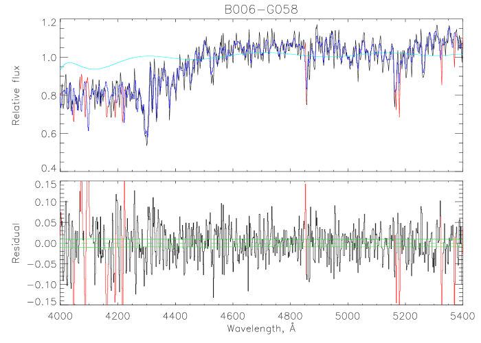
Figure 3: Example ULySS full-spectrum fit for the cluster B006–G058. The top panel shows the observed spectrum in black; the best-fitting spectra fromcthe pegase-hr model is shown in blue; the outliers of the fits are reproduced in red. The cyan lines delineate the multiplicative polynomials. The bottom panels are the fractional residuals of the best fits, where the dashed and solid lines in green denote, respectively, zero and the 1$\sigma$ deviations, with the latter calculated from the (in)variance of the input (observed) spectra.

Figure 4: ULySS fit results: Metallicities versus ages of our sample GCs derived with the spectroscopic fitting. The error bars for both the ages and metallicities are shown in the plots, but they are very small. Left: Vazdekis et al. (2010) SSP models; Right: pegase-hr SSP models.

Figure 5: Same as Fig. 4, but for the Thomas et al. models.

Figure 6: Same as Fig. 4, but for the galev models.

(a) Padova 1994 evolutionary tracks; Chabrier IMF

(b) Padova 1994 evolutionary tracks; Salpeter IMF

(c) Padova 2000 evolutionary tracks; Chabrier IMF

(d) Padova 2000 evolutionary tracks; Salpeter IMF

Figure 7: Metallicities versus ages of our sample GCs derived only from Lick/IDS absorption-line index fits with the Bruzual & Charlot (2003) models, Padova 1994/2000 evolutionary tracks, and Chabrier/Salpeter IMFs.

(a) Padova 1994 evolutionary tracks; Chabrier IMF

(b) Padova 1994 evolutionary tracks; Salpeter IMF

(c) Padova 2000 evolutionary tracks; Chabrier IMF

(d) Padova 2000 evolutionary tracks; Salpeter IMF

Figure 8: Metallicities versus ages of our sample GCs derived only based on SED fitting with the Bruzual & Charlot (2003) models, Padova 1994/2000 evolutionary tracks, and Chabrier/Salpeter IMFs.

(a) Padova 1994 evolutionary tracks; Chabrier IMF

(b) Padova 1994 evolutionary tracks; Salpeter IMF

(c) Padova 2000 evolutionary tracks; Chabrier IMF

(d) Padova 2000 evolutionary tracks; Salpeter IMF

Figure 9: Metallicities versus ages of our sample GCs derived from both the Lick/IDS absorption indices and the SED fits with the Bruzual & Charlot (2003) models, Padova 1994/2000 stellar evolutionary tracks, and Chabrier/Salpeter IMFs.

Figure 10: Comparisons of log( age ) [yr] derived from different models. All $x$ axes are the BC03 (Padova 1994 + Chabrier (2003)) combined fit results to the Lick indices and SEDs. Regarding the $y$ axes, top left: BC03 (Padova 1994 + Chabrier (2003)) fits to only the Lick indices; top right: BC03 (Padova 1994 + Chabrier (2003)) fits to only the SEDs; middle left: BC03 (Padova 2000 + Chabrier (2003)) combined fitting of Lick indices and SEDs; middle right: galev model fitting to only the Lick indices; bottom left: Thomas et al. (2011) fitting of only the Lick indices; bottom right: ULySS models and Vazdekis full-spectrum fitting.

Figure 11: Comparisons of metallicities $\rm[Fe/H]$ derived from different models. Layout and panel coding: same as Fig. 10.

References

- Alves-Brito et al. (2009) Alves-Brito, A., Forbes, D. A., Mendel, J. T., Hau, G. K. T., & Murphy, M. T. 2009, MNRAS, 395, L34
- Ashman & Bird (1993) Ashman, K. M., & Bird, C. M. 1993, AJ, 106, 2281
- Ashman et al. (1994) Ashman, K. M., Bird, C. M., & Zepf, S. E. 1994, AJ, 108, 2348
- Barmby et al. (2000) Barmby, P., Huchra, J., Brodie, J., et al. 2000, AJ, 119, 727
- Barmby & Huchra (2001) Barmby, P., & Huchra, J. P. 2001, AJ, 122, 2458
- Bono et al. (1997) Bono, G., Caputo, F., Cassisi, S., Castellani, V., & Marconi, M. 1997, ApJ, 489, 822
- Bruzual & Charlot (2003) Bruzual A., G., & Charlot, S. 2003, MNRAS, 344, 1000
- Caldwell et al. (2009) Caldwell, N., Harding, P., Morrison, H., et al. 2009, AJ, 137, 94
- Caldwell et al. (2011) Caldwell, N., Schiavon, R., Morrison, H., Rose, J., & Harding, P. 2011, AJ, 141, 61
- Cardiel et al. (1998) Cardiel, N., Gorgas, J., Cenarro, J. & Gonzalez, J. J. 1998, A&AS, 127, 597
- Cardelli et al. (1989) Cardelli, J. A., Clayton, G. C., & Mathis, J. S., 1989, ApJ, 345, 245
- Cassisi et al. (1997) Cassisi, S., Castellani, M., & Castellani, V. 1997, A&A, 317, 10
- Chabrier (2003) Chabrier, G., 2003, PASP, 115, 763
- Chen et al. (2016) Chen, B. Q., Liu, X. W., Xiang, M. S., et al. 2016, AJ, 152, 45
- Eggen et al. (1962) Eggen, O. J., Lynden-Bell, D., & Sandage, A. R. 1962, ApJ, 136, 748
- Fan et al. (2006) Fan, Z., Ma, J., de Grijs, R., Yang, Y., & Zhou, X. 2006, MNRAS, 371, 1648
- Fan et al. (2008) Fan, Z., Ma, J., de Grijs, R., & Zhou, X. 2008, MNRAS, 385, 1973
- Fan et al. (2010) Fan, Z., de Grijs, R., & Zhou, X. 2010, ApJ, 725, 200
- Fan et al. (2011) Fan, Z., Huang, Y. F., Li, J. Z., et al. 2011, RAA, 11, 1298
- Fan et al. (2012) Fan, Z., Huang, Y. F., Li, J. Z., et al. 2012, RAA, 12, 829
- Fan & de Grijs (2012) Fan, Z., & de Grijs, R., 2012, MNRAS, 424, 2009
- Fan & de Grijs (2014) Fan, Z., & de Grijs, R., 2014, ApJS, 211, 22
- Fan et al. (2016) Fan, Z., Wang, H. J., Jiang, X. J., et al., 2016, PASP, in press (arXiv:1605.09166)
- Frogel et al. (1980) Frogel, J. A., Persson, S. E., & Cohen J. G. 1980, ApJ, 240, 785
- Galleti et al. (2004) Galleti, S., Federici, L., Bellazzini, M., Fusi Pecci, F., & Macrina, S. 2004, A&A, 426, 917
- Galleti et al. (2006) Galleti, S., Federici, L., Bellazzini, M., Buzzoni, A., & Fusi Pecci, F. 2006, A&A, 456, 985
- Galleti et al. (2009) Galleti, S., Bellazzini, M., Buzzoni, L., Federici, L.,& Fusi Pecci, F. 2009, A&A, 508, 1285
- Graves & Schiavon (2008) Graves, G. J., & Schiavon, R. P. 2008, ApJS, 177, 446
- Girardi (2000) Girardi, L., Bressan, A., Bertelli, G., & Chiosi, C. 2000, A&AS, 141, 371
- Huchra et al. (1991) Huchra J. P., Brodie J. P., & Kent S. M. 1991, ApJ, 370, 495
- Huchra et al. (1982) Huchra, J. P., Stauffer, J., & van Speybroeck, L. 1982, ApJ, 259, L57
- Huxor et al. (2004) Huxor, A., Tanvir, N. R., Irwin, M. J., et al. 2004, in ASP Conf. Ser. 327, Satellites and Tidal Streams, ed. F. Prada, D. Martinez-Delgado, & T. Mahoney (San Francisco: ASP), p. 118
- Huxor et al. (2005) Huxor, A. P., Tanvir, N. R., Irwin, M. J., et al. 2005, MNRAS, 360, 1007
- Huxor (2007) Huxor, A. 2007, Ph.D. Thesis, Univ. of Hertfordshire, UK
- Huxor et al. (2011) Huxor, A. P., Ferguson, A. M. N., Tanvir, N. R., et al. 2011, MNRAS, 414, 770
- Kotulla et al. (2009) Kotulla, R., Fritze, U., Weilbacher, P., & Anders, P., 2009, MNRAS, 396, 463
- Koleva et al. (2009) Koleva, M., Prugniel, Ph., Bouchard, A., & Wu, Y. 2009, A&A, 501, 1269
- Le Borgne et al. (2004) Le Borgne, D., Rocca-Volmerange, B., Prugniel, P., et al., 2004, A&A, 425, 881
- Li & Han (2008) Li, Z.-M., & Han, Z.-W. 2008, ApJ, 685, 225
- Li et al. (2013) Li, Z.-M., Mao, C.-Y., Chen, L., Zhang, Q., Li, M.-C. 2013, ApJ, 776, 37
- Lilly & Fritze-v. Alvensleben (2006) Lilly, T., & Fritze-v. Alvensleben, U. 2006, A&A, 457, 467
- Ma et al. (2007) Ma, J., Yang, Y. B., Burstein, D., et al. 2007, ApJ, 659, 359
- Ma et al. (2009) Ma, J., Fan, Z., de Grijs, R., et al. 2009, AJ, 137, 4884
- Ma et al. (2010) Ma, J., Wu, Z., Wang, S., et al. 2010, PASP, 122, 1164
- Ma et al. (2011) Ma, J., Wang, S., Wu, Z., et al. 2011, AJ, 141, 86
- Mackey et al. (2006) Mackey, A. D., Huxor, A., Ferguson, A. M. N., et al. 2006, ApJ, 653, L105
- Mackey et al. (2007) Mackey, A. D., Huxor, A., Ferguson, A. M. N., et al. 2007, ApJ, 655, L85
- Mackey et al. (2010) Mackey, A. D., Ferguson, A. M. N., Irwin, M. J., et al. 2010, MNRAS, 401, 533
- Maraston (2005) Maraston, C. 2005, MNRAS, 362, 799
- Maraston (1998) Maraston, C. 1998, MNRAS, 300, 872
- Massey et al. (1988) Massey, P., Strobel, K., Barnes, J. V., & Anderson, E. 1988, ApJ, 328, 315
- McConnachie et al. (2005) McConnachie, A. W., Irwin, M. J., Ferguson, A. M. N., et al. 2005, MNRAS, 356, 979
- McConnachie et al. (2009) McConnachie, A. W., Irwin, M. J., Ibata, R. A., Dubinski, J., & Widrow, L. M. 2009, Nature, 461, 66
- Peacock et al. (2010) Peacock, M. B., Maccarone, T. J., Knigge, C., et al. 2010, MNRAS, 402, 803
- Peng et al. (2006) Peng, E., Cote, P., Jordan, A., et al. 2006, ApJ, 639, 838
- Perina et al. (2010) Perina, S., Cohen, J. G., Barmby, P., et al. 2010, A&A, 511, 23
- Perrett et al. (2002) Perrett, K. M., Bridges, T. J., Hanes, D. A., et al. 2002, AJ, 123, 2490
- Prugniel & Soubiran (2001) Prugniel, Ph. & Soubiran, C., 2001, A&A, 369, 1048
- Prugniel et al. (2007) Prugniel, Ph., Soubiran, C., Koleva, M., Le Borgne, D. 2007, arXiv:astro-ph/0703658
- Racine (1991) Racine, R. 1991, AJ, 101, 865
- Salpeter (1955) Salpeter, E. E. 1955, ApJ, 121, 161
- Sánchez-Blázquez et al. (2006) Sánchez-Blázquez, P., Peletier, R. F.; Jiménez-Vicente, J., et al. 2006, MNRAS, 371, 703
- Searle & Zinn (1978) Searle, L., & Zinn, R. 1978, ApJ, 225, 357
- Sharina et al. (2006) Sharina, M. E., Afanasiev, V. L., & Puzia, T. H. 2006, MNRAS, 372, 1259
- Thomas et al. (2003) Thomas, D., Maraston, C., & Bender, R. 2003, MNRAS, 339, 897
- Thomas et al. (2004) Thomas, D., Maraston, C., & Korn, A. 2004, MNRAS, 351, L19
- Thomas et al. (2011) Thomas, D., Maraston, C., & Johansson, J. 2011, MNRAS, 412, 2183
- van den Bergh (1969) van den Bergh, S. 1969, ApJS, 19, 145
- Vazdekis et al. (2010) Vazdekis, A., Sánchez-Blázquez, P., Falcón-Barroso, J., et al. 2010, MNRAS, 404, 1639
- Wang et al. (2010) Wang, S., Fan, Z., Ma, J., de Grijs, R., & Zhou, X. 2010, AJ, 139, 1438
- Worthey et al. (1994a) Worthey, G., Faber, S. M., Gonzalez, J. J., & Burstein, D. 1994, ApJS, 94, 687
- Worthey (1994b) Worthey, G. 1994, ApJS, 95, 107
- Worthey & Ottaviani (1997) Worthey, G., &Ottaviani, D. L. 1997, ApJS, 111, 377