Continuum Kinetic and Multi-Fluid Simulations of Classical Sheaths

Abstract

The kinetic study of plasma sheaths is critical, among other things, to understand the deposition of heat on walls, the effect of sputtering, and contamination of the plasma with detrimental impurities. The plasma sheath also provides a boundary condition and can often have a significant global impact on the bulk plasma. In this paper, kinetic studies of classical sheaths are performed with the continuum kinetic code, Gkeyll, that directly solves the Vlasov-Maxwell equations. The code uses a novel version of the finite-element discontinuous Galerkin (DG) scheme that conserves energy in the continuous-time limit. The fields are computed using Maxwell equations. Ionization and scattering collisions are included, however, surface effects are neglected. The aim of this work is to introduce the continuum kinetic method and compare its results to those obtained from an already established finite-volume multi-fluid model also implemented in Gkeyll. Novel boundary conditions on the fluids allow the sheath to form without specifying wall fluxes, so the fluids and fields adjust self-consistently at the wall. The work presented here demonstrates that the kinetic and fluid results are in agreement for the momentum flux, showing that in certain regimes, a multi-fluid model can be a useful approximation for simulating the plasma boundary. There are differences in the electrostatic potential between the fluid and kinetic results. Further, the direct solutions of the distribution function presented here highlight the non-Maxwellian distribution of electrons in the sheath, emphasizing the need for a kinetic model. Densities, velocities, and potential show good agreement between the kinetic and fluid results. However, kinetic physics is highlighted through higher moments such as parallel and perpendicular temperatures which provide significant differences from the fluid results in which the temperature is assumed to be isotropic. Besides decompression cooling, the heat flux is shown to play a role in the temperature differences that are observed, specially inside the collisionless sheath.

I Introduction

When plasma is contained by walls, the boundaries behave as sinks. Due to their high thermal velocity (in comparison to heavier ions) electrons are quickly absorbed into the wall, which leads to the creation of a typically positive space charge region called a sheath.Robertson (2013) The resulting potential barrier works to equalize fluxes to the wall. Even though the sheath width is usually on the order of a Debye length, $\lambda_{D}$, it plays an important role in particle, momentum, energy and heat transfer, and surface erosion, which can, in turn, have a global effect on the plasma. Furthermore, field-accelerated ions and hot electrons are known to cause an emission from the solid surface that can further alter the system. Therefore, the sheath must be self-consistently included and resolved in numerical simulations. This significantly affects a computational cost of simulations, because the scale length of the system is usually several orders of magnitude higher than the Debye length. Usually, the effect of the sheath is mimicked with “sheath boundary conditions”, often constructed from very simple flux balance arguments or making assumptions like cold ions and no surface effects.Loizu et al. (2012) Hence, first-principle simulations of the sheath are needed to both validate and further develop the simple models as well as to understand the global kinetic effects of sheaths on the bulk plasma.

Sheath physics has been studied since early the works of Langmuir,Langmuir (1923) but some processes remain to be fully understood. The original criterion for a shielding sheath, commonly known as the Bohm criterionBohm (1949) is given by

$$u^{2}_{i,0}\geq\frac{\text{k}_{\text{B}}T_{e}}{m_{i}},$$ (1)

where $u_{i,0}$ is the ion bulk velocity perpendicular to the wall at the sheath edge. The Bohm criterion assumes mono-energetic ions, Boltzmann electrons, and no sources in the plasma, and does not depend on the ion distribution function at the edge. Effectively, it assumes a single-component fluid with ion inertia and electron pressure. The Bohm criterion then requires for ions to be accelerated in the presheath to the speed of ion acoustic waves.Riemann (1990) Surprisingly, even with the assumptions mentioned above, the Bohm criterion applies to conditions beyond these assumptions, with errors within 20 - 30 %.Bohm (1949)

Kinetic effects (ions are no longer monoenergetic but are rather distributed over the velocity space; electrons no longer instantly follow the electrostatic potential) are incorporated in the Tonks-Langmuir model with the solution presented in Ref [Harrison and Thompson, 1959]. This “kinetic Bohm criterion” is discussed and generalized in several papersAllen (1976); Bissell and Johnson (1987); Riemann (1990, 1995); Fernsler, Slinker, and Joyce (2005); Riemann (2006) and its applicability on different plasma distribution functions is further addressed.Baalrud and Hegna (2011); Riemann (2012); Baalrud and Hegna (2012) An alternative approach based on the fluid moment hierarchy is presented in recent work.Baalrud et al. (2015) The latter approach leads to a sheath criterion that is similar to the original Bohm criterion but contains an extra term for the ion temperature.

When the energy of incident particles is high enough, bounded electrons in the wall can be ejected, and the boundary begins acting as a source of plasma. This mechanism, known as secondary electron emission (SEE), is critical for devices like Hall thrustersDunaevsky, Raitses, and Fisch (2003) and tokamak walls.Takamura et al. (2004) Particle-in-cell (PIC) simulationsSydorenko and Smolyakov (2004); Sydorenko et al. (2006) show that the electron distribution function in Hall thrusters is, due to the SEE, strongly anisotropic and depletes at high energies. Therefore, a kinetic approach is required. Further discussion of kinetic effects, plasma flux to the wall, secondary electron fluxes, plasma potential, and electron cross-field conductivity are presented in Ref [Kaganovich et al., 2007]. Recent workCampanell, Khrabrov, and Kaganovich (2012) studies conditions for sheath instability due to SEE and “weakly confined electrons” at the boundary of the loss cone.

PIC simulations and Direct Simulation Monte-Carlo (DSMC) are currently the most widely used methods for kinetic scales. They are robust, allow complex geometries, and can include a broad range of physical and chemical processes. However, PIC simulations are subject to noise – an issue that can be overcome by using continuum kinetic solvers with high-order accurate algorithms. Also, simulations of complex problems like Hall thrusters have relevant scales from the magneto-hydrodynamic (MHD) scale to the kinetic scale and efficiently resolving all of them is computationally expensive. Continuum kinetic solvers potentially allow easier implementation of hybrid (fluid-kinetic) algorithms for problems requiring such a scale separation, and enable the use of novel multi-scale techniques like asymptotic preserving methodsEmako and Tang (2016); Liu and Xu (2016) that self-consistently transition between the regimes without changing the underlying equations or implementation.

Here the focus is on directly solving the Boltzmann equation,

$$\frac{\partial f}{\partial t}+\textbf{v}\cdot\frac{\partial f}{\partial\textbf{x}}+\frac{q}{m}\left(\textbf{E}+\textbf{v}\times\textbf{B}\right)\frac{\partial f}{\partial\textbf{v}}=S,$$ (2)

using a discontinuous Galerkin (DG) scheme.Cockburn and Shu (2001) Here, $f(\mathbf{x},\mathbf{v},t)$ is the particle distribution function, $q$ is charge, $m$ is mass and $S$ represents different source terms. A continuum Eulerian scheme is used in this work. DG schemes have been extensively developed and used in the computational fluid dynamics and applied mathematics community over the past 15 years, as they combine some of the advantages of finite-element schemes (low phase error, high accuracy, flexible geometries) with finite-volume schemes (limiters to preserve positivity/monotonicity, locality of computation for parallelization).

The kinetic DG results are compared to results from a two-fluid finite-volume scheme.Hakim, Loverich, and Shumlak (2006) The two-fluid model uses novel boundary conditions that compute fluxes self-consistently using Riemann solvers at the wall. Therefore, the fluxes to the wall are a result of the model rather than input parameters. This work demonstrates an agreement between kinetic and fluid solutions in density and momentum for several regimes. The sheath potential differs on order of 10%, and the difference is more pronounced as ion temperature becomes significant. More significant differences are observed in the temperature profiles. The kinetic results, performed using one configuration space dimension and two velocity space dimensions, produce parallel ($x$-direction) and perpendicular electron temperatures that differ significantly from the isotropic fluid temperature. This difference is attributed to the parallel heat flux, not present in the five-moment two-fluid model. Furthermore, the smooth distribution function profiles obtained from the kinetic model highlight the non-Maxwellian nature of the species distribution inside the sheath. This is a fundamental difference between kinetic and fluid sheath simulations as fluid models assume a Maxwellian distribution throughout.

This paper is organized as follows. Section II provides a short review of sheath theory and the Bohm criterion. Section III covers the continuum kinetic model and section IV briefly describes the electromagnetic five-moment two-fluid model. Benchmarking of the code with simulations of the Weibel instability is presented in section V. Problem setup and initial conditions are discussed in section VI. Comparison between kinetic and fluid models is provided in section VII and finally section VIII summarizes this work and outlines future plans.

II Brief review of sheath theory

Langmuir’s two-scale descriptionLangmuir (1923) is used here, which assumes a quasi-neutral presheath and a sheath region with non-zero space charge. This description is valid as long as $\lambda_{D}/L\ll 1$. The dimensionless parameters in this section are consistent with previous publications,Riemann (1990)

$$y =\frac{m_{i}v_{i}^{2}}{2\text{k}_{\text{B}}T_{e}}, \chi =-\frac{e\phi}{\text{k}_{\text{B}}T_{e}},$$

$$n_{e,i} =\frac{N_{e,i}}{N_{0}}, \xi =\frac{x}{\lambda_{D}},$$

where $N_{e,i}$ are electron and ion number densities and $N_{0}$ is charged particle number density at the sheath edge (same for electrons and ions in the $\lambda_{D}/L\rightarrow 0$ approximation). The simulations use a slightly modified set of variables that are more suitable for practical implementation. The classical Bohm criterion ($y_{0}\geq\frac{1}{2}$) can then be derived from the ion continuity equation, $n_{i}y^{1/2}=y_{0}^{1/2}$, ion energy conservation $y=y_{0}+\chi$, Boltzmann electron density $n_{e}=\text{exp}(-\chi)$, and the Poisson equation $\text{d}^{2}\chi/\text{d}\xi^{2}=n_{i}-n_{e}$.Riemann (1990)

Since the Bohm criterion applies a boundary condition on the ion drift speed, there is a need for a mechanism that would accelerate ions in the presheath. This mechanism is described as an ambipolar diffusion with nonlinear effects caused by the ion inertia.Persson (1962)

Equating the ion density with the electron Boltzmann factor,

$$n_{i}\sqrt{y}=j_{i},\quad j_{i}=\left(\frac{m_{i}}{2\text{k}_{\text{B}}T_{e}}\right)^{1/2}\frac{J_{i}}{N_{0}}$$ (3)

where $J_{i}$ is ion current density gives

$$\frac{\text{d}y}{\text{d}\zeta}-\frac{\text{d}\chi}{\text{d}\zeta}<\frac{1}{j_{i}}\frac{\text{d}j_{i}}{\text{d}\zeta},$$ (4)

for the presheath ($y_{0}<\frac{1}{2}$). Here $\zeta=x/L$ where $L$ is a characteristic scale in the system.

From Eq. (4) and the conservation of energy, $y=y_{0}+\chi$, the acceleration to the Bohm velocity is possible only ifRiemann (1990)

1. $\text{d}j_{i}/\text{d}\zeta>0$ and/or

2. $\text{d}y/\text{d}\zeta<\text{d}\chi/\text{d}\zeta$.

These conditions can be fulfilled by several mechanisms. Relevant to this work are the collisional presheath and ionizing presheath. The collisional presheath introduces ion friction and therefore fulfills $\mathrm{d}y/\mathrm{d}\zeta<\mathrm{d}\chi/\mathrm{d}\zeta$ with $L$ being ion mean free path. The ionizing presheath satisfies both the increase in current gradient condition, $\text{d}j_{i}/\text{d}\zeta>0$, and ion retardation because the particles created by ionization are assumed to have zero drift velocity. In this case, $L$ corresponds to the mean ionization path. The model presented here includes both scattering collisions and electron impact ionization.

Ref [Baalrud et al., 2015] emphasizes that the concept of a sheath edge in Langmuir’s description is connected strictly to the charge density and therefore should be independent of a plasma model (an example of a description that is dependent on a plasma model is the Child-Langmuir formula). Instead they suggest identifying the sheath edge using a threshold for the normalized charge density $\bar{\rho}_{c}=(n_{i}-n_{e})/n_{i}$. However, in a real situation where $\lambda_{D}/L\neq 0$ this transition is not abrupt, hence, arbitrary values must be chosen. In the results presented using the continuum kinetic model, the thresholds for $\bar{\rho}_{c}=1$ % and 10 % are marked by arrows. By taking the expansion of $\rho$ with respect to $\phi$, the quantitative form of the sheath condition is derived,Baalrud et al. (2015)

$$\left|\frac{\mathrm{d}n_{i}}{\mathrm{d}x}\right|\leq\left|\frac{\mathrm{d}n_{e}}{\mathrm{d}x}\right|.$$ (5)

The density gradients required for Eq. (5) can be obtained from the steady Boltzmann equation leading to a slightly modified version of the classical Bohm criterionBaalrud et al. (2015)

$$u_{i}\geq v_{\mathrm{B}}=\sqrt{\frac{\mathrm{k}_{\mathrm{B}}\left(T_{e}+T_{i}\right)-m_{e}v_{e}^{2}}{m_{i}}}.$$ (6)

III Continuum kinetic model

III.1 Numerical method

An energy-conserving, discontinuous Galerkin (DG) scheme is used to discretize the Valsov-Maxwell equations. The time-derivative term is discretized with a strong-stability preserving Runge-Kutta scheme. In the time-continuous limit, with a specific choice of numerical flux for Maxwell equations, the scheme can be shown to conserve total (particle plus field) energy. Although momentum is not conserved exactly, the errors in momentum conservation are independent of velocity space resolution and converge rapidly with increasing configuration space resolution. While developing the code significant numerical advance have been made, allowing efficient solution of the Vlasov-Maxwell (and hybrid moment-Vlasov-Maxwell) systems. These developments will be presented in a forthcoming paper.

III.2 Ionization and collision terms

Discussion in section II shows that adding an ionizing source term can provide a steady-state.Riemann (1990) A simplified version of electron impact ionization is derived from the exact operator of the formMeier and Shumlak (2012)

$$S_{ion,s}=f_{n}(\textbf{v})\int_{-\infty}^{\infty}\sigma(|\textbf{v}-\textbf{v}^{\prime}|)|\textbf{v}-\textbf{v}^{\prime}|f_{e}(\textbf{v}^{\prime})\mathrm{d}\textbf{v}^{\prime},$$ (7)

where $\sigma(|\textbf{v}-\textbf{v}^{\prime}|)$ is the ionization differential cross-section with units of $[L]^{2}$. Assuming the electron thermal velocity is high in comparison to the relative bulk speed, the relative speed, $|\textbf{v}-\textbf{v}^{\prime}|$, can be approximated by the electron random velocity. The formula then simplifies to

$$S_{ion,s}\approx f_{n}(\textbf{v})\left\langle\sigma v_{e}\right\rangle n_{e},$$ (8)

where $\left\langle\sigma v_{e}\right\rangle$ is the value averaged over the velocity space.

The neutral distribution is assumed to be a non-drifting bi-Maxwellian

$$f_{BM,s}=\frac{n_{s}}{\sqrt{2\pi v_{thx,s}^{2}}\sqrt{2\pi v_{thy,s}^{2}}}e^{\frac{-v_{x}^{2}}{2v_{thx,s}^{2}}}e^{\frac{-v_{y}^{2}}{2v_{thy,s}^{2}}},$$ (9)

that does not get depleted during the course of the simulation. Assuming that species created by ionization are thermalized on time-scales shorter than other collision times, and the neutral number density is not a function of time, Eq. (8) is rewritten as

$$S_{ion,s}=\left\langle\sigma v_{r}\right\rangle n_{n}f_{BM}\left(n_{e},\,0,\,\textbf{v}_{th,s}\right).$$ (10)

On the right-hand-side there is a distribution function with local number density of electrons, zero drift velocity, and local temperature of respected species.

The ionization rate, $\left\langle\sigma v_{r}\right\rangle$ in Eq. (10), is selected so as to achieve a quasi-steady-state. Using a cold ion and Boltzmann electron model, a simple balance of ionization sources and particle loss at the walls shows that to achieve steady-state the ionization rate must beStangeby (2000)

$$\left\langle\sigma v_{r}\right\rangle=\frac{2u_{B}}{L}\left(\frac{\pi}{2}-1\right),$$ (11)

where the factor of 2 corresponds to the two-wall setup with particles leaving the domain on both sides (see section VI for more details). Even though this result is derived using significant approximations, including even a simple ionization term helps with density conservation. Fig. 1 presents the relative total number density as a function of time for ions and electrons in one of our sheath simulations. After the simulation has progressed for 4000 plasma oscillation times ($1/\omega_{pe}$), the relative difference in initial and final integrated number densities in the simulation for both species is less than 5%. Even though the number of particles is not conserved exactly, adding this physics-based source term could lead to some results, that are otherwise unobservable (for example the positive sheath transition described in the Ref [Campanell and Umansky, 2016]). However, achieving the true steady-state with this approach requires a calculation of the inelastic collision integrals and inclusion of the surface physics effects.

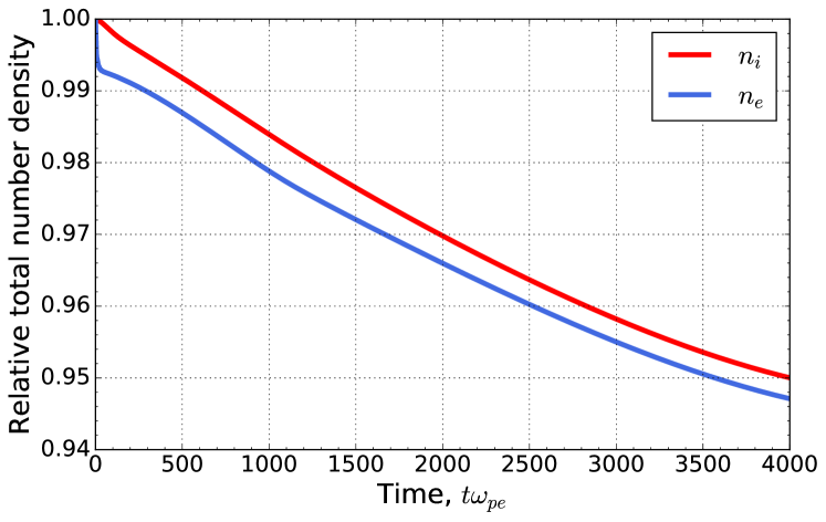
Figure 1: Relative integrated number densities of electrons and ions evolved over $4000/\omega_{pe}$, showing that the ionization and collision terms nearly balance.

To balance the loss of high-energy electrons to the walls, collisions must be included to replenish the electron tails if steady-state is to be achieved. These collisions, however, should be infrequent enough that the collisional mean-free-path is much longer than the sheath width, allowing for proper simulation of collisionless sheaths. The presented work uses a simple BGKBhatnagar, Gross, and Krook (1954) operator

$$S_{coll,s}=\nu_{coll}\left(f_{M,s}-f_{s}\right),$$ (12)

where $f_{M,s}$ is a Maxwellian distribution function, which is constructed using the first three moments of $f_{s}$. The temperature of the distribution is taken as $(T_{x}+2T_{\perp})/3$. Collision frequency $\nu_{coll}$ is calculated locally as

$$\nu_{coll,ss}=\frac{e^{4}}{2\pi\epsilon_{0}^{2}m_{s}^{2}}\frac{n_{s}}{v_{th,s}^{3}}\mathrm{ln}(\Lambda).$$ (13)

Local values of density, $n_{s}$, and thermal velocity, $v_{th,s}$, are used. The Coulomb logarithm is approximated as $\mathrm{ln}(\Lambda)=10$. Note that the mass has a power of 2, which is caused by the fact that thermal velocities are used instead of temperatures. Interspecies collisions are neglected in this work. With this setup, the collision frequency decreases as plasma enters the sheath region. Using the initial values for electrons, the electron-electron collision frequency near the wall is around 0.3 $\omega_{pe0}$.

IV Electromagnetic five-moment two-fluid model

The two-fluid plasma model is included for comparison with the continuum kinetic simulation. It includes electron inertia, separate electron and ion temperatures, and allows for non-neutral effects (which are crucial for obtaining Debye sheaths). The fields are computed from the full Maxwell equations, which allows for the inclusion of displacement currents. Each species of the plasma is described by moments of a distribution function – number density, momentum, and energyHakim, Loverich, and Shumlak (2006)

$$\frac{\partial n_{s}}{\partial t}+\frac{\partial}{\partial x}\left(n_{s}u_{x}\right)=0,$$ (14)

$$m\frac{\partial n_{s}u_{x}}{\partial t}+\frac{\partial}{\partial x}\left(p_{s}+m_{s}n_{s}u_{x}^{2}\right)=n_{s}q_{e}E_{x},$$ (15)

$$\frac{\partial\mathcal{E}_{s}}{\partial t}+\frac{\partial}{\partial x}\left(u_{x}p_{s}+u_{x}\epsilon_{s}\right)=q_{s}n_{s}u_{x}E_{x},$$ (16)

where $p_{s}$ is the isotropic pressure for each species and $E_{x}$ is the electric field. To close the system, heat flow is neglected and a scalar closure is used for the energy $\epsilon_{s}$

$$\epsilon_{s}=\frac{p_{s}}{\gamma-1}+\frac{1}{2}n_{s}u_{x}^{2},$$ (17)

where $\gamma=\frac{5}{3}$.

To solve the system of five-moment equations, a second order, locally implicit scheme is used. This scheme is partly described in Ref. [Hakim, Loverich, and Shumlak, 2006; Loverich et al., 2013]. Using a locally implicit, operator splitting approach, the time-step restriction due to the plasma frequency and Debye length scales can be eliminated. This decreases the computational time for multi-fluid simulations, especially with realistic electron/ion mass ratios, even when using an explicit scheme. For the hyperbolic homogeneous part of the equations, a finite-volume (FV) wave-propagation scheme is used.LeVeque (2002) This scheme is based on solving the Riemann problem at each interface to compute numerical fluxes, which are then used to construct a second-order scheme. To ensure that the number density remains positive, on detection of a negative density/pressure state, the homogeneous step is recomputed using a diffusive, but positive, Lax-flux.Bouchut (2004) Although Lax-flux adds diffusion, the scheme still conserves particles and energy.

To apply boundary conditions at the walls, a vacuum is assumed just outside the domain (i.e. just inside the wall the plasma is neutralized and the fields vanish). This introduces a jump in the fluids and electric field, which is then used in a Riemann solver to compute the self-consistent fluxes corresponding to that jump. This ensures that the solution automatically adjusts to give the correct surface fluxes and fields, and one does not need to specify the flux using the Bohm criteria, as is usually done in fluid codes. In codes that use “ghost cells” for the boundary conditions, this BC is particularly easy to implement: one simply sets the fluid quantities to zero and then uses the scheme’s Riemann solver to compute the surface fluxes that are then used to update the cell adjacent to the wall.

V Benchmarking kinetic and fluid models with Weibel instability

As the algorithms are developed, systematic benchmarking exercises are performed. The detailed description of the algorithms and benchmarks for the kinetic code will be published in the future. Versions of the kinetic algorithms, applied to the quasi-neutral gyrokinetic equations have been benchmarked.Shi, Hakim, and Hammett (2015) The fluid code has also been thoroughly tested, as well as used in production runs for magnetic reconnection,Wang et al. (2015); Ng et al. (2015) global magnetosphere simulations, Rayleigh-Taylor instability, and other problems. Both the fluid and kinetic algorithms are implemented in the Gkeyll code, and use common infrastructure for input/output, parallelization, simulation drivers and output visualization. Gkeyll also has advanced fluid models, including the ten-moment modelHakim (2008) with a local as well as non-local closure, a gyrokinetic model, and a full Vlasov-Maxwell solver. This opens up the possibility of performing hybrid sheath simulations in the future, with some particle species evolved using fluids, while others evolved with a kinetic or reduced kinetic model.

A benchmark comparison (against analytical theory as well as between models) for the WeibelWeibel (1959) instability is presented here. The Weibel instability is potentially relevant to sheath formation in some regimes,Tang (2011) which motivates its selection as a benchmark here. Furthermore, this problem highlights the unique features of the five-moment fluid code used here to capture particular kinetic effects by the inclusion of multiple “streams” of a single species, in this case, the electrons.

The Weibel instability is driven by anisotropic pressure, an example of which occurs in the presence of two counter-streaming electron beams. When a small perturbation of magnetic field is introduced perpendicular to the relative drift velocity, the Weibel instability causes this magnetic field to grow exponentially. In the linear regime, the dispersion relation for this instability takes the form

$$\frac{1}{2}=\frac{\omega_{0}^{2}}{c^{2}k^{2}}\left[\zeta Z(\zeta)\left(1+\frac{v_{D}^{2}}{v_{th}^{2}}\right)+\frac{v_{D}^{2}}{v_{th}^{2}}\right]+\frac{v_{th}^{2}}{c^{2}}\zeta^{2},$$ (18)

where $\omega_{0}$ is the plasma oscillation frequency, $c$ is the speed of light, $k$ is the instability wavenumber, $v_{D}$ is the populations drift speed, and $v_{th}$ is thermal speed, $\zeta=\omega/(\sqrt{2}v_{th}k)$, where $\omega=\omega_{r}+\mathrm{i}\gamma$. $Z(\zeta)$ is the plasma dispersion function defined as

$$Z(\zeta)=\frac{1}{\sqrt{\pi}}\int_{-\infty}^{\infty}\frac{e^{-x^{2}}}{x-\zeta}\mathrm{d}x.$$ (19)

In the cold fluid limit, using the asymptotic expansion of $Z(\zeta)$ for large $\zeta$, the cold fluid Weibel dispersion relation is obtained

$$\frac{{\omega}^{4}}{2{k}^{2}}-\left(\frac{1}{2}+\frac{1}{{k}^{2}}\right){\omega}^{2}-v_{D}^{2}=0$$ (20)

where $\omega$ is normalized to $\omega_{0}$, $k$ is normalized to $\omega_{0}/c$ and $v_{D}$ is normalized to $c$. This relation is identical to Eq. 12 in Ref [Califano, Pegoraro, and Bulanov, 1997] for the case of two counter-streaming, but otherwise identical electron beams. In contrast to the growth rates predicted from the kinetic dispersion relation, Eq. 18, the cold fluid dispersion relation predicts a larger growth rate.

This problem requires a 3-dimensional computational domain for the kinetic simulations to retain two velocity dimensions (1X2V). The simulation is initialized with two homogeneous counter-streaming populations of electrons and a neutralizing ion background (which is not evolved during the course of simulation). The initial magnetic field is perturbed, using a mode with wavenumber $k$. The configuration space is periodic with a domain size of one wavelength of the initial perturbation.

Previous work with cold fluid modelsPegoraro et al. (1996); Califano et al. (1998) suggests that the simulations should evolve into smaller and smaller spatial scales and create magnetic field singularities. On the other hand, the presented kinetic and two-fluid models include thermal effects and therefore should resolve those scale lengths and saturate when the electron gyroradius decreases to the scale of electron skin depth.Davidson et al. (1972); Califano et al. (1998)

The simulations presented in this work are run with dimensionless parameters – light speed $c=1$, electron temperature $T_{e}=0.01$, Debye length $\lambda_{D}=0.1$, and initial drift $v_{D}=\pm 0.3$. Evolution of the instability is observed in the magnetic field energy plot in Fig. 2.

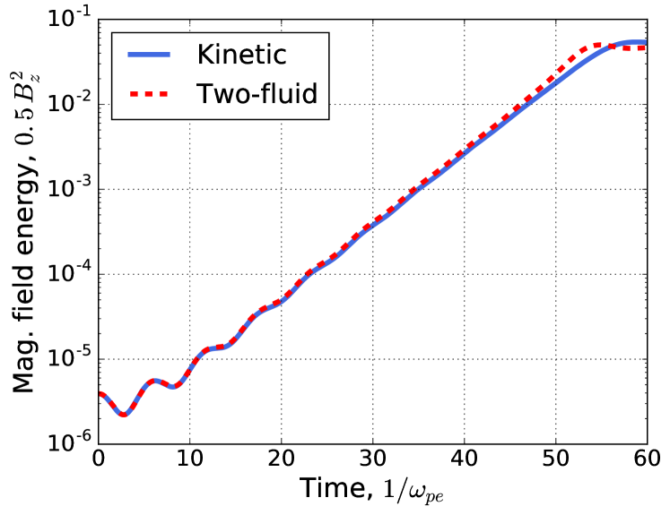
Figure 2: Growth of magnetic field energy due to the homogeneous Weibel instability. In this simulation two counter-streaming electron beams are perturbed by a small magnetic field with $k\lambda_{D}=0.04$. The fluid and kinetic models show similar linear growth, as well as saturate around $55/\omega_{pe}$ to comparable energy levels.

For $k\lambda_{D}=0.04$ the saturation of the instability occurs around $55/\omega_{pe}$ for both kinetic and fluid models. Growth rates, calculated by fitting an exponential function to the energy profile, are within 4 % of each other and from the linear theory prediction. An adaptive algorithm is used for the fit by continuously expanding the fitting region and selecting the region which produces the fit with the highest coefficient of determination, $R^{2}$. This coefficient is defined as $R^{2}=1-\sum_{i}(y_{i}-f_{i})^{2}/\sum(y_{i}-\bar{y})^{2}$, where $y_{i}$ are data points and $f_{i}$ are values of the fitted function. Results for different $k$ are in Fig. 3.

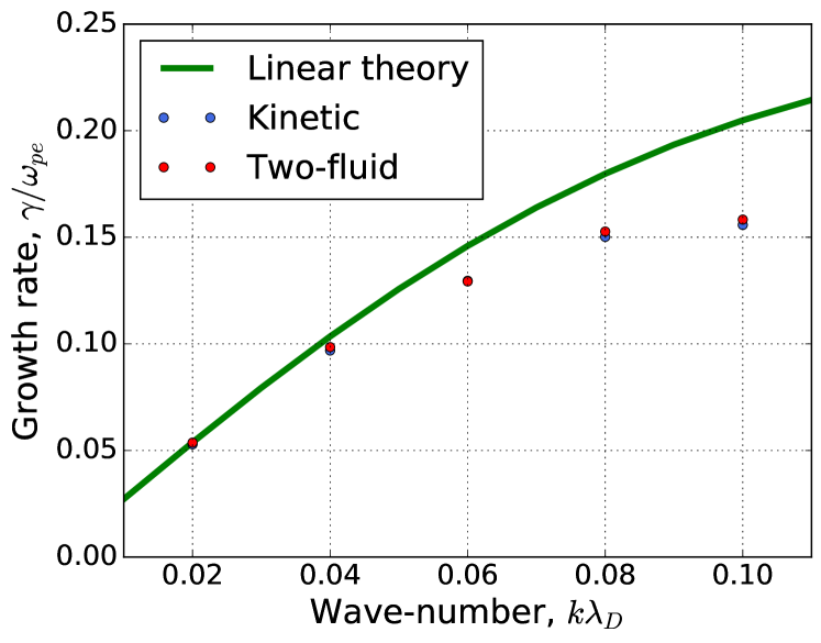
Figure 3: Comparison of the Weibel instability growth rates for the collisionless kinetic code, two-fluid code, and the linear theory prediction (Eq. 18). Note that the initial value of thermal velocity is used in the linear theory dispersion relation (Eq. 18) while the simulation results show an increase in temperature (higher temperature corresponds to lower growth rate). Hence, the lack of agreement for both fluid and kinetic results for high-$k$ modes is linked to the increase in temperature.

Further study of the Weibel instability shows that plasma temperature increases in the course of the instability growth. This increase could explain the difference between the simulation results and the dispersion relation (Eq. 18) prediction, which uses the initial value of particle thermal velocity. For fixed $k$ and drift velocity, the growth rate produced by the dispersion relation decreases with increasing thermal velocity. Detailed analysis of the Weibel instability is beyond the scope of this work. Further analysis of these results and of the Weibel instability in magnetized sheaths will be presented in the future.

VI Problem setup and initial conditions

It is possible to simulate a sheath in one configuration space and only one velocity space dimension (1X1V). This setup, however, does not capture the different evolution of parallel and perpendicular temperatures. To accurately model the anisotropic temperature profiles, a perpendicular temperature evolution equation

$$\frac{\partial}{\partial t}\left(nT_{\perp}\right)+\frac{\partial}{\partial x}\left(u_{x}nT_{\perp}\right)=\nu n\left(T-T_{\perp}\right)$$ (21)

needs to be solved along with the Vlasov equation. $T_{\perp}$ in the Eq. (21) stands for the temperature perpendicular to the flow. Eq. (21) describes the advection of the perpendicular temperature and its isotropization to parallel temperature due to collisions.

Alternatively, one may perform simulations in one configuration space and two velocity space dimensions (1X2V) where the perpendicular temperature is evolved self-consistently. The simulation results presented in this paper are performed using 1X2V. Absorbing walls are modeled on both configuration space boundaries, and this is referred to as a two-wall setup. While this approach doubles the simulation cost and provides no additional information, the one-wall setup, where one domain boundary is a free-edge and the other is an absorbing wall, is very sensitive to the free-edge boundary condition and can lead to unphysical results.

The configuration space ranges from -128 $\lambda_{D}$ to 128 $\lambda_{D}$, and it is divided into 256 cells. The second-order serendipity spaceArnold and Awanou (2011) is used for discretization inside each cell. Second-order polynomials correspond to three internal degrees of freedom and therefore, the Debye length is well resolved. A realistic mass ratio of 1836 is used which requires a different velocity space discretization for each species. The electron velocity domain ranges from -6 to 6 initial electron thermal speed (which is equal to $6\sigma$ of the distribution) and ion velocity domain ranges from -5 to 5 initial Bohm speed. The velocity space for both species is divided into 16 cells. This resolution is chosen based on a grid convergence study using 8, 16, 32, and 64 cells, with converged results obtained for 16 cells.

For consistency with the kinetic simulations, the configuration space of two-fluid simulations has the same range from $-128\,\lambda_{D}$ to $128\,\lambda_{D}$ but is divided into 500 cells. The simulation is initialized with the same density, momentum, and energy profiles as the kinetic model. Moments of the ionization and collision terms are included as sources in the fluid model.

The two-wall setup allows a simplified set of boundary conditions. Dirichlet boundary conditions, $\phi=0$, are used for the electrostatic potential at both boundaries. At the velocity space boundaries, the particle flux is set to zero, allowing conservation of total particle density in the domain. At the walls, the particles streaming into the wall are completely absorbed. The wall boundary conditions can hence be written as $f(-L/2,v_{x},v_{\perp},t)=0$ for $v_{x}>0$, and $f(L/2,v_{x},v_{\perp},t)=0$ for $v_{x}<0$.

As mentioned in Sec. II, simulations use a slightly modified set of normalized variables. Even though normalization of density to the density at the sheath edge is useful for theoretical work, the simulation results presented here use initial undisturbed density as the normalization.

A natural choice would be to initialize the simulation with a uniform distribution in the configuration space and let the sheath evolve self-consistently. This, however, leads to problems in reaching steady state. The electric field does not appear in the presheath instantly. As a consequence, no mechanism would accelerate the ions from the presheath towards the wall. The ionization is, however, still in effect and the number density in the presheath grows over the initial value. Without density gradients or an electric field the first moment of the Boltzmann equation (2) simplifies to $\partial n_{s}/\partial t=n_{e}\cdot C$, where $C$ is an constant independent of $n_{e}$. This implies that when there is an imbalance, the number density growth is exponential. Furthermore, the initial lack of particle flow from the presheath leads to rapid depletion of the sheath region.

Alternatively, one may initialize the simulation with a simplified model and let it settle into a new equilibrium with kinetic effects. Ref [Robertson, 2013] describes a model based on the assumptions of mono-energetic ions, Boltzmann electrons, and uniform ionization rate, $R$, over the whole domain. The validity of the last assumption is arguable, because the ionization rate should depend on the electron number density,Meier and Shumlak (2012) which changes significantly in the sheath region and is generally decreasing in the presheath. This model is described (in dimensionless units) by the ion momentum equation,

$$\frac{\mathrm{d}\tilde{u}(x)}{\mathrm{d}\tilde{x}}=\frac{\tilde{E}(x)}{\tilde{u}(x)}-\frac{\tilde{R}}{\tilde{n}_{i}(x)},$$ (22)

the Poisson equation,

$$\frac{\mathrm{d}\tilde{E}(x)}{\mathrm{d}\tilde{x}}=\frac{\tilde{J}_{i}(x)}{\tilde{u}_{i}(x)}-e^{\tilde{\phi}(x)},$$ (23)

and the relation between the field and the potential,

$$\frac{\mathrm{d}\tilde{\phi}(x)}{\mathrm{d}\tilde{x}}=-\tilde{E}(x).$$ (24)

These equations can then be integrated from the middle of the domain towards the walls to get the density [$\tilde{n}_{i}=\tilde{R}\tilde{x}/\tilde{u}$ and $\tilde{n}_{e}=\mathrm{exp}(\tilde{\phi})$] and bulk velocity profiles. These profiles are then used to initialize a Maxwellian distribution with preset uniform thermal velocities.

Using these initial conditions, in the first few electron plasma oscillation times ($1/\omega_{pe}$), excess electrons quickly leave the domain and fluxes are equalized. This behavior results in excitation of waves that travel through the domain, leading to an oscillation of potential. This behavior has been noted in other works.Lieberman and Lichtenberg (2005) Spectral analysis shows that the waves are electron waves oscillating at exactly the plasma oscillation frequency $\omega_{pe}$. An advantage of the initial conditions mentioned above is that starting with the approximate solution significantly limits the excitation of these electron waves and averaging over several plasma periods is no longer necessary.

Phase-space plots of distributions ($xv_{x}$-planes of 1X2V distributions) are presented in Fig. 4 (ions) and Fig. 5 (electrons) using the described model for initial conditions.Robertson (2013) These figures show smooth distribution function profiles for each of the species. The velocity space domain that is used is sufficient to capture the majority of the distribution function for each of the species including the ion distribution in the ion acceleration region. Note some key features of sheath physics captured here – electron trapping near the wall and ion acceleration both in the sheath and presheath.

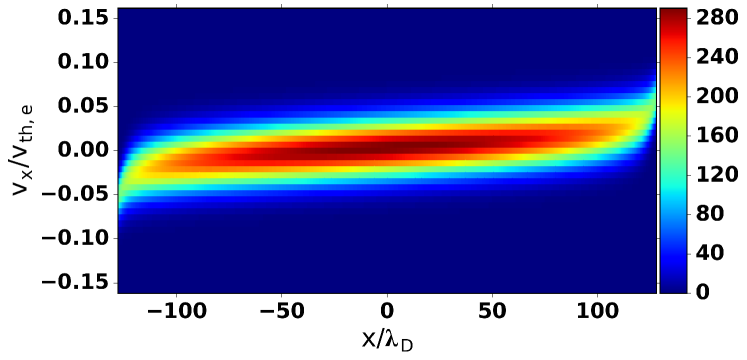
Figure 4: $xv_{x}$-plane of the ion distribution function evolved over $200/\omega_{pe}$. In this setup, there are perfectly absorbing walls on both boundaries of the configuration space. This figure shows a noise-free solution of the ion population getting accelerated by the sheath electric field. Initial temperature ratio $T_{0e}/T_{0i}=1$ and a realistic mass ratio $m_{e}/m_{i}=1/1836$ are used. The sheath potential accelerates the ions to supersonic speeds, adjusting to match the electron flux to give a net zero current.

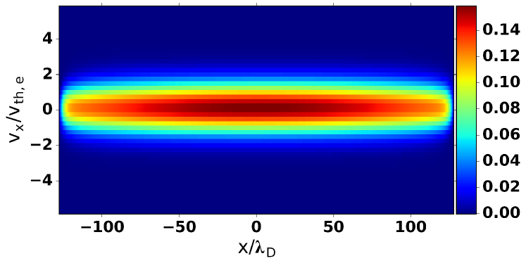
Figure 5: Same as Fig. 4, expect for electrons. The electrons are confined by the sheath potential, with the high energy electrons lost to the walls.

VII Discussion and comparison of models

As mentioned previously, continuum kinetic methods provide access to the full distribution function everywhere in the domain. Hence, one can directly plot the distribution function at any point in space to study any deviations from a Maxwellian distribution that may exist. The distribution function cross-section for the electrons is plotted in Fig. 6 with and without the ionization sources and collisions at two different times. Simulations marked as RHS=0 in the figure are performed without both collisions and ionization. All lines are for an initial temperature ratio of $T_{0,e}/T_{0,i}=1$. Solutions are shown for two different times, 50$/\omega_{pe}$ and 100$/\omega_{pe}$. The distribution functions are plotted at the right domain boundary; hence, positive velocity in this plot denotes the outflow of electrons. In the presence of sources, the part of the distribution function that lies in the positive velocity region is Maxwellian early and late in time. The part of the distribution function that lies in the negative velocity region is non-Maxwellian, and the sharp gradient in the distribution occurs due to fast electrons leaving the domain and slower electrons being reflected by the electrostatic potential. The vertical green line in the plot shows a speed corresponding to the electrostatic energy, $v=\sqrt{2e\phi/m_{e}}$. Simulations without the sources exhibit different behavior, particularly late in time. Without sources, the solution (dark blue dashed line) at 50$/\omega_{pe}$ resembles the case with sources i.e. Maxwellian distribution in the positive velocity region and abrupt drop in the distribution in the negative velocity region. However the later-time solution at 100$/\omega_{pe}$ (cyan dashed-line) starts to show non-Maxwellian features in the positive velocity region of the distribution function as well. In the absence of collisions and ionization, the fast electrons leave the domain, and the information propagates through the entire domain before showing up in the distribution function on the positive velocity region of this plot at the right boundary. When collisions and ionization are included, the electron distribution gets thermalized in the bulk plasma as a result of which it remains Maxwellian in the positive velocity region. The negative velocity region of the distribution function on the right wall is not affected by the inclusion of sources (not forced to fluid-like Maxwellian) whereas the positive velocity region is significantly altered by them. The smoothing of the negative velocity region of the distribution function could be caused by numerical dissipation or it could be an inherent effect of time marching schemes. Detailed investigation of this feature is deferred to the future work.

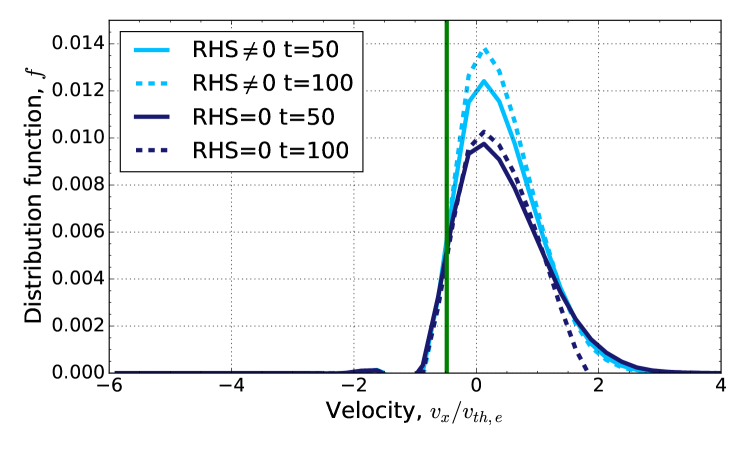
Figure 6: Electron distribution function cross-section ($v_{x}$) at a distance of $\lambda_{D}/3$ from the right wall. Two simulation results – with collisions and ionization (RHS$\neq$0) and without either (RHS=0) – are plotted here at two times, 50$/\omega_{pe}$ and 100$/\omega_{pe}$. The velocity corresponding to the electrostatic potential at this location is plotted as a green line. Note that the distribution is in the simulation captured from -6 $v_{th,e}$ to 6 $v_{th,e}$.

To explore the macroscopic effects of this kinetic behavior, the continuum kinetic and fluid simulations are compared for several temperature ratios. The summarizing plots of the ion momentum to the wall, non-neutral region width, and electric potential drop over this region evolved for 200$/\omega_{pe}$ are presented in Fig. 7. It is not straightforward to the define the non-neutral region width, because the difference in number densities of the species is introduced continuously. Instead, 1% difference is arbitrary chosen and the distance of this point from the wall is taken as the non-neutral region width.

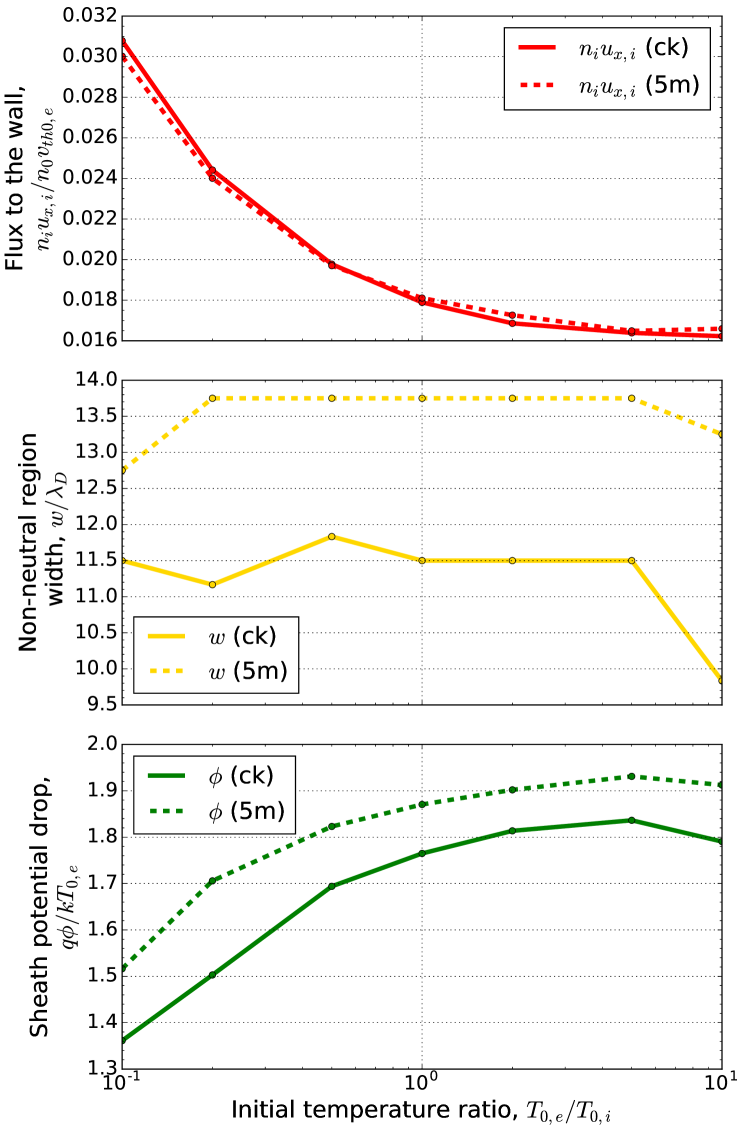
Figure 7: Comparison of the flux to the wall (Top), non-neutral region width (Middle); defined by the 1 % difference between electron and ion densities), and electric potential drop over this region (Bottom) versus the initial temperature ratio between the continuum kinetic (ck) and five-moment two-fluid (5m) models. See Tab. 1 for quantitative comparison. Simulations are evolved from initial conditions for 200$/\omega_{pe}$.

Figure 7 shows that the kinetic and fluid models provide good agreement when comparing flux to the wall at several temperature ratios. The distribution function is non-Maxwellian for electrons that have been reflected by the electrostatic potential. The part of the electron population that is propagating towards the wall still retains the half-Maxwellian distribution. Both models also use a realistic mass ratio and the same temperature ratio between the species. Therefore, it is reasonable to expect the same equalizing ion flow towards the wall after the simulation settles into a quasi-steady-state.

The number density is defined as an integral of the distribution function over the velocity space. In the sheath region near the domain boundaries, the non-Maxwellian distribution function has a sharp gradient in the inflow part of the distribution function. This leads to a difference in sheath electron number density between the kinetic and fluid models and subsequently, affects the sheath edge calculation (marked as the non-neutral region width) as seen in Fig. 7. When the plasma distribution gets thermalized in the bulk plasma, this difference disappears.

The electrostatic potential is compared between the fluid and kinetic models in Fig. 7 for different temperature ratios. Some of this difference is attributed to the difference in the sheath width due to which different physical locations are used to determine the potential. This approach is used because the potential drop over the sheath region is a relevant physical parameter used to characterize sheaths.

The quantitative comparison of kinetic and fluid results are summarized in Table 1 for the same three parameters plotted in Fig. 7, namely, flux to the wall, sheath width, and electrostatic potential. The fluid and kinetic models agree to within about $20\%$ of each other which provides some confidence in the boundary conditions used for the fluids.

$T_{0e}/T_{0i}$	Flux	Sheath width	Potential
0.1	2.4%	10.9%	11.4%
1.0	1.1%	19.5%	5.9%
10.0	2.2%	34.7%	6.8%

Table 1: Difference between the continuum kinetic and two-fluid solutions (defined as $|kinetic-fluid|/kinetic$) for flux to the wall, quasi-neutrality region width (defined by the 1 % difference between electron and ion densities), and electric potential drop over this region. See Fig. 7 for plots. Simulations are evolved from initial conditions for 200$/\omega_{pe}$.

The temperature ratios in the $x$-axis of Fig. 7 are initial values. As particles are created by ionization at the local temperature, the plasma cools with slightly different rates for electrons and ions since there is no source of heating in these simulations.

Detailed profiles of normalized density, velocity, electrostatic potential, and temperatures near the wall are presented in Fig. 8 for $T_{0e}/T_{0i}=1$ and after 200/$\omega_{pe}$. The densities for both species are normalized to the initial density, velocities to the local modified Bohm velocity, $u_{B}=\sqrt{\mathrm{k}_{\mathrm{B}}\left(T_{x,e}+T_{x,i}\right)/m_{i}}$, and the electrostatic potential is normalized to $\mathrm{k}_{\mathrm{B}}T_{0e}$. Locations where the plasma is no longer quasi-neutral (1 % and 10 % difference in electron and ion densities) are marked by arrows, with solid arrows representing locations for the kinetic model and dashed arrows representing locations for the fluid model. It is worth noting here that the crossing of the Bohm speed corresponds to the point with 1% difference in number density. The definition of the sheath width used is, therefore, consistent with classical sheath theory.

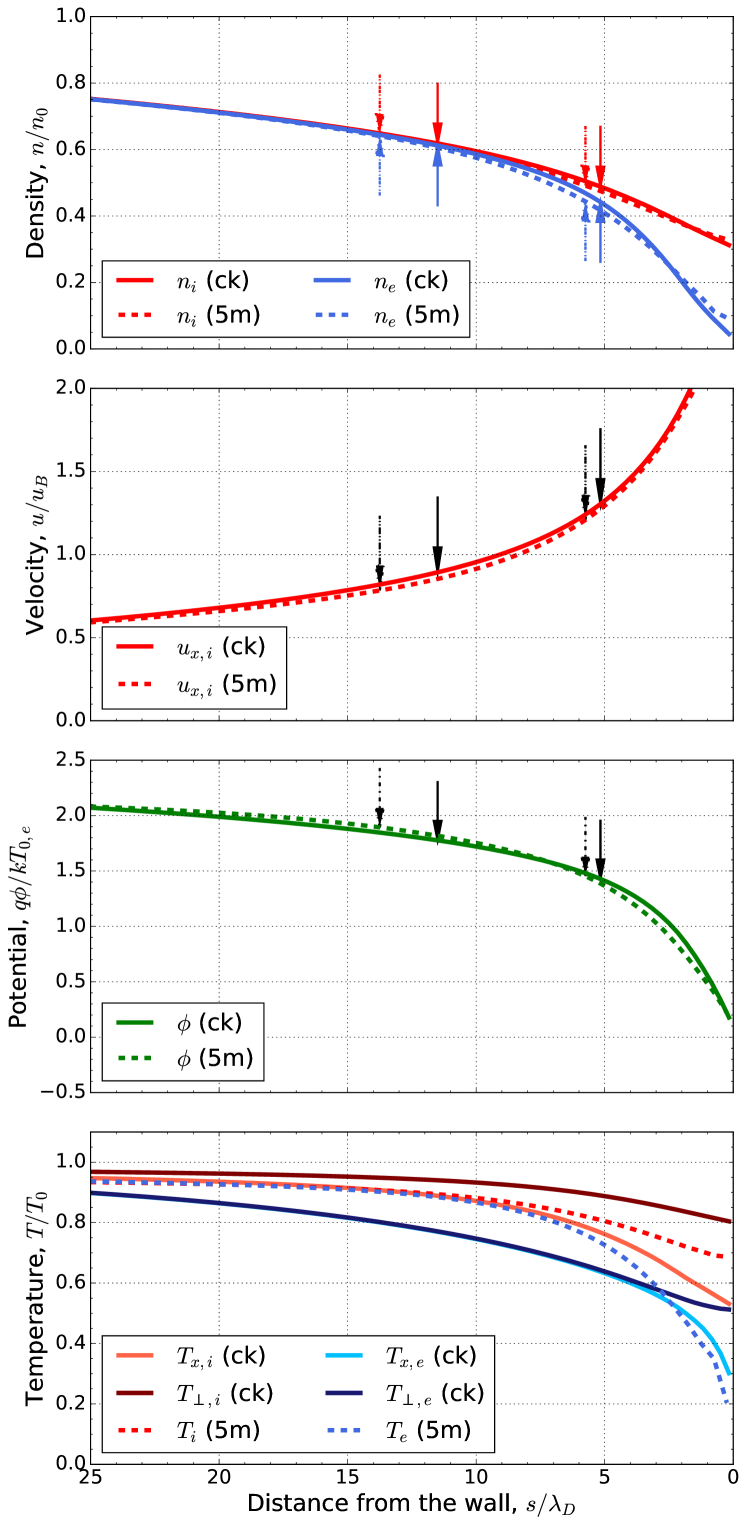
Figure 8: Comparison of continuum kinetic (ck) and five-moment two-fluid (5m) simulations for initial $T_{0e}/T_{0i}=1$. Top Densities are normalized to the initial density in the middle of the domain. Upper middle Velocities normalized to the local modified Bohm velocity ($u_{B}=\sqrt{\mathrm{k}_{\mathrm{B}}\left(T_{x,e}+T_{x,i}\right)/m_{i}}$). Lower middle Electrostatic potentials normalized to $\mathrm{k}_{\mathrm{B}}T_{e}$. Bottom Parallel ($T_{x}$) and perpendicular temperatures. Results of the kinetic code are plotted in the solid line, the two-fluid code in the dashed line. Electron quantities are plotted in blue and ion in red. Arrows show points where a relative difference between electron and ion densities are bigger than 1 % and 10 % (solid arrows correspond to kinetic code, dashed to fluid code). Simulations are evolved from initial conditions for 200$/\omega_{pe}$.

The temperatures plotted in the bottom subfigure of Fig. 8 provide an interesting comparison between fluid and kinetic results and highlight the importance of kinetic effects. The five-moment two-fluid model used here assumes an isotropic temperature. The parallel temperatures ($T_{x}$) for both electrons and ions in the continuum kinetic results undergo decompression cooling as expected.Tang (2011) The parallel temperature is then equalized with the perpendicular temperature through collisions. It is observed that this effect is more apparent for electrons due to their higher collision frequency with respect to ions. The ion temperature is in good agreement between continuum kinetic and fluid simulations (isotropic fluid temperature lies in between the ion parallel and perpendicular). However, the electron temperature has more significant differences between the kinetic and fluid results. To understand this, higher moments are needed. The second moment of the Vlasov equation leads to the energy conservation equation

$$\frac{\partial\mathcal{E}}{\partial t}+\frac{1}{2}\frac{\partial\mathcal{Q}_{iik}}{\partial x_{k}}=nq\textbf{u}\cdot\textbf{E},$$ (25)

where

$$\mathcal{E}=\frac{3}{2}p+\frac{1}{2}mn\mathbf{u}^{2}$$ (26)

is the particle energy and

$$\mathcal{Q}_{ijk}=m\int v_{i}v_{j}v_{k}f\thinspace d^{3}\mathbf{v}.$$ (27)

is the heat flux tensor. Contraction of $\mathcal{Q}_{ijk}$ gives (twice) the particle energy-flux density and can be expanded as follows

$$\frac{1}{2}\mathcal{Q}_{iix}=\underbrace{q_{x}+u_{x}\Pi_{xx}}_{non-ideal}+\underbrace{\frac{5}{2}pu_{x}+\frac{1}{2}mnu_{x}^{3}}_{ideal},$$ (28)

where $\Pi_{xx}$ is the parallel component of the stress tensor, $p$ is pressure, and

$$q_{x}=\frac{1}{2}m\int_{-\infty}^{\infty}\int_{0}^{\infty}\left(w_{x}^{2}+v_{\perp}^{2}\right)w_{x}f(v_{x},v_{\perp})2\pi v_{\perp}dv_{\perp}dv_{x}$$ (29)

is the heat flux vector in the plasma frame, and $w_{x}=v_{x}-u_{x}$. Individual terms of Eq. (28) are plotted in Fig. 9 for the electrons. The decompression cooling terms (green lines) between the kinetic and fluid results are in good agreement and are dominant terms. The five-moment fluid model used here does not capture the kinetic physics of the heat flux vector and the stress tensor. The stress tensor plotted in Fig. 9 (blue line close to zero) is negligible in this case and is not a significant kinetic effect here. The heat flux vector (red line), however, is significant in the sheath. The heat flux vector is negligible in the bulk plasma where the distribution function is thermalized by collisions. Within about $50$ Debye lengths of the wall, however, the heat flux becomes significant and this could explain the differences in electron temperature between the kinetic and fluid results.

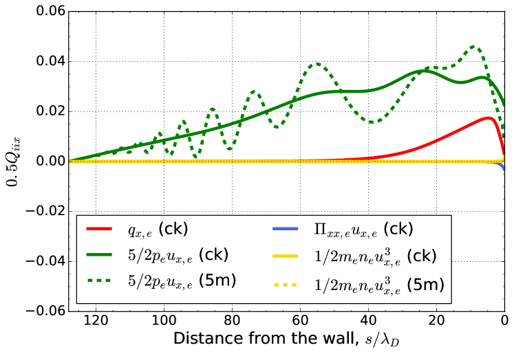
Figure 9: Individual terms of the expanded heat flux (Eq. 28). Heat flux vector in the plasma frame, $q$ and stress tensor are only available in the continuum kinetic simulations (marked as ck). Simulations are evolved from initial conditions for 100$/\omega_{pe}$.

VIII Conclusions

The continuum kinetic solvers using the discontinuous Galerkin scheme in the Gkeyll code might provide access to high-dimensionality simulations and noise-free results which have been inaccessible thus far. Successful benchmarks of the scheme have been performed and compared to previous literature as well as to fluid simulations.

The kinetic and fluid models are benchmarked with the collisionless Weibel instability and good agreement is found. Additionally, the saturation of the fluid Weibel instability is converged and corresponds to the kinetic saturation. The extracted growth rates agree with each other and with the linear theory prediction for small wavenumbers. The mechanism for nonlinear saturation and effect of increasing temperature on linear growth rates will be further explored in future work.

A 1D classical sheath using a two-wall setup is simulated using both the kinetic and two-fluid scheme. The kinetic and two-fluid results are in good agreement for momentum and density of both species over the sheath region (see Table 1 for quantitative comparison), demonstrating that the two-fluid model may be useful in certain regimes to study sheath physics. However, key differences are present when looking at higher moments such as parallel ($T_{x}$) and perpendicular temperatures where the 5-moment fluid model assumes an isotropic temperature. These differences in the temperature are attributed to the heat flux vector, a kinetic effect which is missed in the fluid model. Additionally, the distribution function in the sheath is non-Maxwellian highlighting the need for kinetic physics. The inclusion of further physics and, in particular, magnetic fields oriented at arbitrary angles to the wall may lead to further differences between the fluids and kinetic models due to finite orbit effects, not typically captured completely in the fluid model.

The models described here will be extended to include surface and atomic physics, with more sophisticated collision terms, which are sensitive to the non-Maxwellian shape of the plasma distribution function near the wall, thus requiring a kinetic model. Also, the inclusion of magnetic fields in the kinetic model will provide a tool to study plasma/solid-surface interactions relevant to Hall thrusters, as well as develop parameterized boundary conditions, along the lines of Ref [Loizu et al., 2012], for use in fluid simulations of fusion machines.