Universal hydrodynamic mechanisms for crystallization in active colloidal suspensions

Abstract

The lack of detailed balance in active colloidal suspensions allows dissipation to determine stationary states. Here we show that slow viscous flow produced by polar or apolar active colloids near plane walls mediates attractive hydrodynamic forces that drive crystallization. Hydrodynamically mediated torques tend to destabilize the crystal but stability can be regained through critical amounts of bottom-heaviness or chiral activity. Numerical simulations show that crystallization is not nucleational, as in equilibrium, but is preceded by a spinodal-like instability. Harmonic excitations of the active crystal relax diffusively but the normal modes are distinct from an equilibrium colloidal crystal. The hydrodynamic mechanisms presented here are universal and rationalize recent experiments on the crystallization of active colloids.

DOI: 10.1103/PhysRevLett.117.228002

In active colloidal suspensions Palacci et al. (2013); Petroff et al. (2015), energy is continuously dissipated into the ambient viscous fluid. The balance between dissipation and fluctuation that prevails in equilibrium colloidal suspensions Einstein (1905); Kubo (1966) is, therefore, absent. Nonequilibrium stationary states in active suspensions, then, are determined by both dissipative and conservative forces, quite unlike passive suspensions where detailed balance prevents dissipative forces from determining phases of thermodynamic equilibrium. In this context, it is of great interest to enquire how thermodynamic phase transitions driven by changes in free energy are modified in the presence of sustained dissipation.

In two recent experiments disordered suspensions of active colloids have been observed to spontaneously order into two-dimensional hexagonal crystals when confined at a plane wall. Bottom-heavy synthetic active colloids which catalyze hydrogen peroxide when optically illuminated are used in the first experiment Palacci et al. (2013) while chiral fast-swimming bacteria of the species Thiovulum majus are used in the second experiment Petroff et al. (2015). Given this remarkably similar crystallization in two disparate active suspensions it is natural to ask if the phenomenon is universal and to search for mechanisms, necessarily involving dissipation, that drive it.

Our current understanding of phase separation in particulate active systems is derived from the coarse-grained theory of motility-induced phase separation (MIPS) where active particles are advected by a density-dependent velocity Tailleur and Cates (2008); Cates et al. (2010); Cates and Tailleur (2013, 2015). Microscopic models with kinematics consistent with MIPS also show phase separation and crystallization of hard active disks have been reported in two dimensions Henkes et al. (2011); Fily and Marchetti (2012); Bialké et al. (2012); Redner et al. (2013). However, these models ignore exchange of the locally conserved momentum of the ambient fluid with that of the active particles and are, thus, best applied to systems where such exchanges can be ignored. Fluid flow is an integral part of the physics in Palacci et al. (2013); Petroff et al. (2015) and a momentum-conserving theory, currently lacking, is essential to identify the dissipative forces and torques that drive crystallization.

In this Letter we present a microscopic theory of active crystallization that connects directly to the experiments described above. Specifically, we account for the three-dimensional active flow in the fluid and the effect of a plane wall on this flow. Representing activity by slip in a thin boundary layer at the colloid surface Ghose and Adhikari (2014); Singh et al. (2015); Singh and Adhikari (2016) we rigorously compute the long-ranged many-body hydrodynamic forces and torques on the colloids. Thus we estimate Brownian forces and torques to be smaller than their active counterparts by factors of order $10^{2}$ (for synthetic colloids in Palacci et al. (2013)) to $10^{4}$ (for bacteria in Petroff et al. (2015)) making them largely irrelevant for active crystallization. We integrate the resulting deterministic balance equations numerically to obtain dynamical trajectories.

Our main numerical results are summarized in Fig. (1). Panels (a)-(c) show the spontaneous destabilization of the uniform state by attractive active hydrodynamic forces, the formation of multiple crystallites, and their coalescence into a single hexagonal crystal at late times. Panels (d)-(f) show the structure factor at corresponding times. The route to crystallization is not through activated processes that produce critical nuclei, but through a spinodal-like instability produced by the unbalanced long-ranged active attraction. The uniform state is, therefore, always unstable and crystallization occurs for all values of density, in contrast to the finite density necessary for crystallization in MIPS models Cates and Tailleur (2015). Active hydrodynamic torques tend to destabilize the ordered state but stability is regained when these are balanced by external torques (from bottom-heaviness in Palacci et al. (2013)) or by chiral activity (from bacterial spin in Petroff et al. (2015)). Crystallites of chiral colloids rotate at an angular velocity that is inversely proportional to the number of colloids contained in them, as shown in panel (g). This is in excellent agreement with the experiment Petroff et al. (2015). The critical values of bottom-heaviness and chirality above which orientational stability, and, hence, positional order, is ensured is shown in panel (h). We now present our model and detail the derivation of our results.

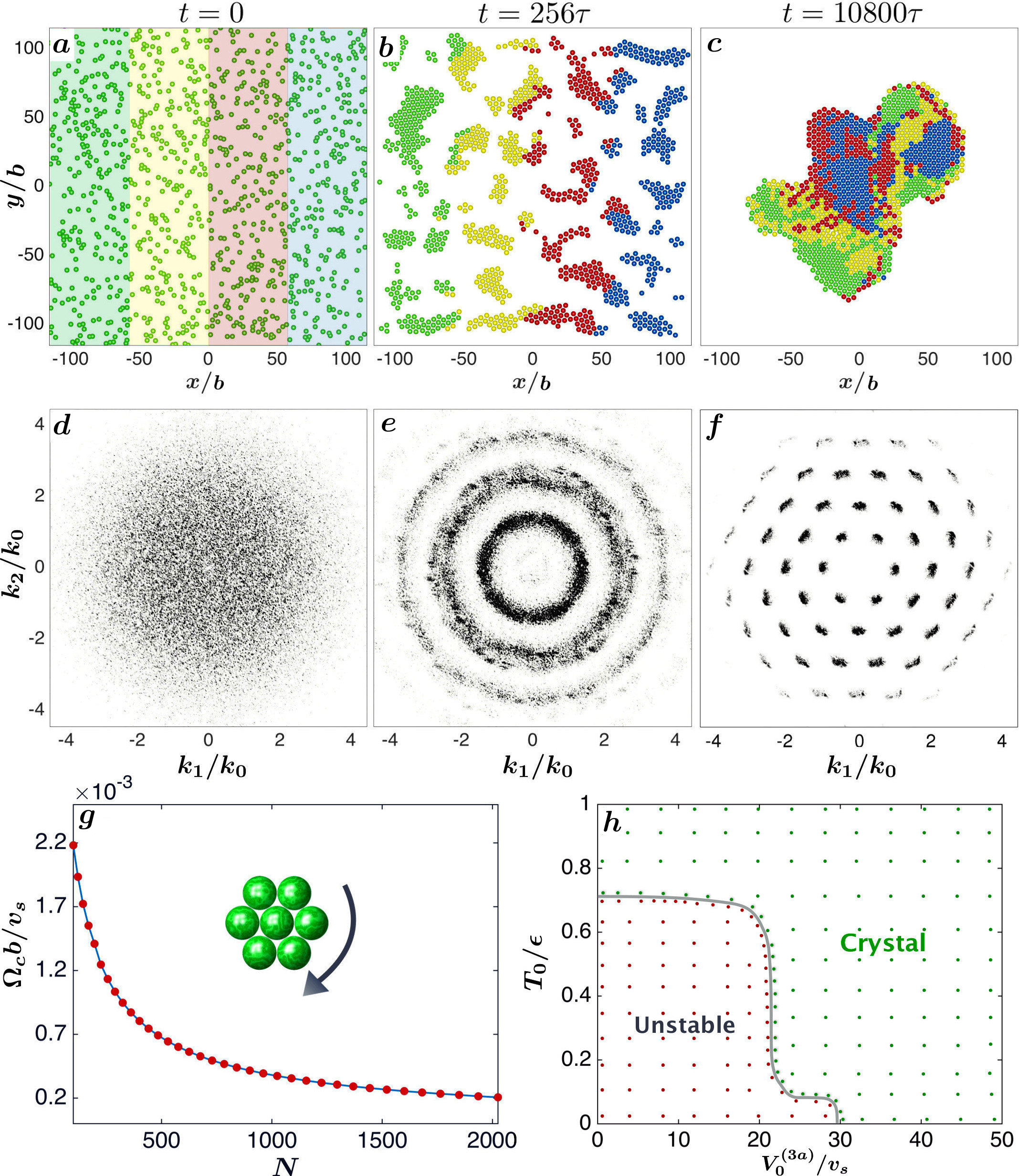
Figure 1: Panels (a)-(c) are instantaneous configurations during the crystallization of $1024$ active colloids of radius $b$ at a plane wall. The colloids are colored by their initial positions. Panels (d)-(f) show the structure factor $S(\mathbf{k})$ at corresponding instants. Wavenumbers are scaled by the modulus of the reciprocal lattice vector $k_{0}$ and the contribution from $\mathbf{k}=0$ is discarded. Panel (g) shows the variation of the angular velocity $\mathbf{\Omega}_{c}$ of a crystallite with the number $N$ of colloids in it. A typical configuration is shown in the inset. Panel (h) is the state diagram for orientational stability in terms of the measure of chirality $V_{0}^{(3a)}$ and bottom-heaviness $T_{0}$ (see text). Each dot represents one simulation. Here $v_{s}$ is the self-propulsion speed of an isolated colloid, $\tau=b/v_{s}$, and $\epsilon$ is the scale of the repulsive steric potential.

Model: We consider $N$ spherical active colloids of radius $b$ near a plane wall with center-of-mass coordinates $\mathbf{R}_{i},$ orientation $\mathbf{p}_{i}$, linear velocity $\mathbf{V}_{i}$, and angular velocity $\boldsymbol{\Omega}_{i}$, where $i=1\ldots N$. Activity is imposed through a slip velocity $\mathbf{v}_{i}^{\mathcal{A}}$ which is a general vector field on the surface $S_{i}$ of the $i$-th colloid satisfying $\int{\bm{\hat{\rho}}_{i}\cdot}\mathbf{v}_{i}^{\mathcal{A}}\,d\text{S}_{i}=0$ sli , where $\boldsymbol{\rho}_{i}$ is the vector from the center of the colloid to a point on its surface. The fluid velocity $\mathbf{v}$ is subject to slip boundary conditions

$$\mathbf{v}(\mathbf{R}_{i}+\boldsymbol{\rho}_{i})=\mathbf{V}_{i}+\bm{\Omega}_{i}\times\bm{\rho}_{i}+\mathbf{v}_{i}^{\mathcal{A}}(\bm{\rho}_{i}).$$ (1)

on the colloid surfaces, to a no-slip boundary condition $\mathbf{v}=0$ at the plane wall located at $z=0$, and to a quiescent boundary condition at large distances from the wall. The slip is conveniently parametrized by an expansion $\mathbf{v}^{\mathcal{A}}(\mathbf{R}_{i}+\boldsymbol{\rho}_{i})=\sum_{l=1}^{\infty}\tfrac{1}{(l-1)!(2l-3)!!}\,\mathbf{V}_{i}^{(l)}\cdot\mathbf{Y}^{(l-1)}(\bm{\hat{\rho}}_{i})$ in irreducible tensorial spherical harmonics $\mathbf{Y}^{(l)}(\bm{\hat{\rho}})=(-1)^{l}\rho^{l+1}\bm{\nabla}{}^{(l)}\rho^{-1}$, where $\bm{\nabla}^{(l)}=\bm{\nabla}_{\alpha_{1}}\dots\bm{\nabla}_{\alpha_{l}}$. The expansion coefficients $\mathbf{V}_{i}^{(l)}$ are $l$-th rank reducible Cartesian tensors with three irreducible parts of ranks $l,$ $l-1,$ and $l-2$, corresponding to symmetric traceless, antisymmetric and pure trace combinations of the reducible indices. We denote these by $\mathbf{V}_{i}^{(ls)}$, $\mathbf{V}_{i}^{(la)}$ and $\mathbf{V}_{i}^{(lt)}$ respectively. The leading contributions from the slip,

$$\mathbf{v}_{i}^{\mathcal{A}}(\bm{\rho}_{i}) = \underbrace{-\mathbf{V}_{i}^{\mathcal{A}}+\tfrac{1}{15}\mathbf{V}_{i}^{(3t)}\cdot\mathbf{Y}^{(2)}}_{\mathrm{achiral,\,polar}}-\underbrace{\tfrac{1}{9}\boldsymbol{\varepsilon}\cdot\mathbf{V}_{i}^{(3a)}\cdot\mathbf{Y}^{(2)}}_{\mathrm{chiral,\thinspace apolar}}$$ (2)

$$+ \underbrace{\mathbf{V}_{i}^{(2s)}\cdot\mathbf{Y}^{(1)}}_{\mathrm{achiral,\,apolar}}-\underbrace{\mathbf{\Omega}_{i}^{\mathcal{A}}\times\bm{\rho}_{i}-\tfrac{1}{60}\boldsymbol{\varepsilon}\cdot\mathbf{V}_{i}^{(4a)}\cdot\mathbf{Y}^{(3)}}_{\mathrm{chiral,\,polar}}$$

have coefficients of polar, apolar and chiral symmetry. Here $\boldsymbol{\varepsilon}$ is the Levi-Civita tensor. The retained modes have physical interpretations: for a single colloid in an unbounded fluid, $\mathbf{V}^{\mathcal{A}}$ ($l\sigma=1s)$ and $\bm{\Omega}^{\mathcal{A}}$ $(l\sigma=2a)$ are the linear and angular velocities in the absence of external forces and torques, $\mathbf{V}^{(2s)}$ is the active contribution to the stresslet, while $\mathbf{V}^{(3a)},\mathbf{V}^{(3t)}$, and $\mathbf{V}^{(4a)}$ are strengths of the chiral torque dipole, polar vector quadrupole, and chiral octupole respectively. The tensors are parametrized uniaxially, $\mathbf{V}_{i}^{\mathcal{A}}=v_{s}\mathbf{p}_{i}$, $\mathbf{\boldsymbol{\Omega}}_{i}^{\mathcal{A}}=\omega_{s}\mathbf{p}_{i}$, ${\bf V}_{i}^{(2s)}=V_{0}^{(2s)}(\mathbf{p}_{i}\mathbf{p}_{i}-\tfrac{\mathbf{I}}{3})$ and so on, where $v_{s}$ and $\omega_{s}$ are the speeds of active translation and rotation and $V_{0}^{(2s)}$ positive (negative) corresponds to a pusher (puller). The relation of these modes to exterior fluid flow and Stokes multipoles is explained in sup .

The synthetic active colloids in Palacci et al. (2013) are polar and achiral (they self-propel but do not spin) while the bacteria in Petroff et al. (2015) are polar and chiral (they self-propel and spin). Both these cases are included in the leading contributions. In Ghose and Adhikari (2014) a procedure is outlined for estimating the leading coefficients from experimentally measured flows and it is shown that the active flow produced by flagellates and green algae can be modeled by slip. Our model is of sufficient generality, then, to include both synthetic and biological active colloids, and situations where swirling and time-dependent slip may be necessary Drescher et al. (2010, 2011); Guasto et al. (2010); Goldstein (2015).

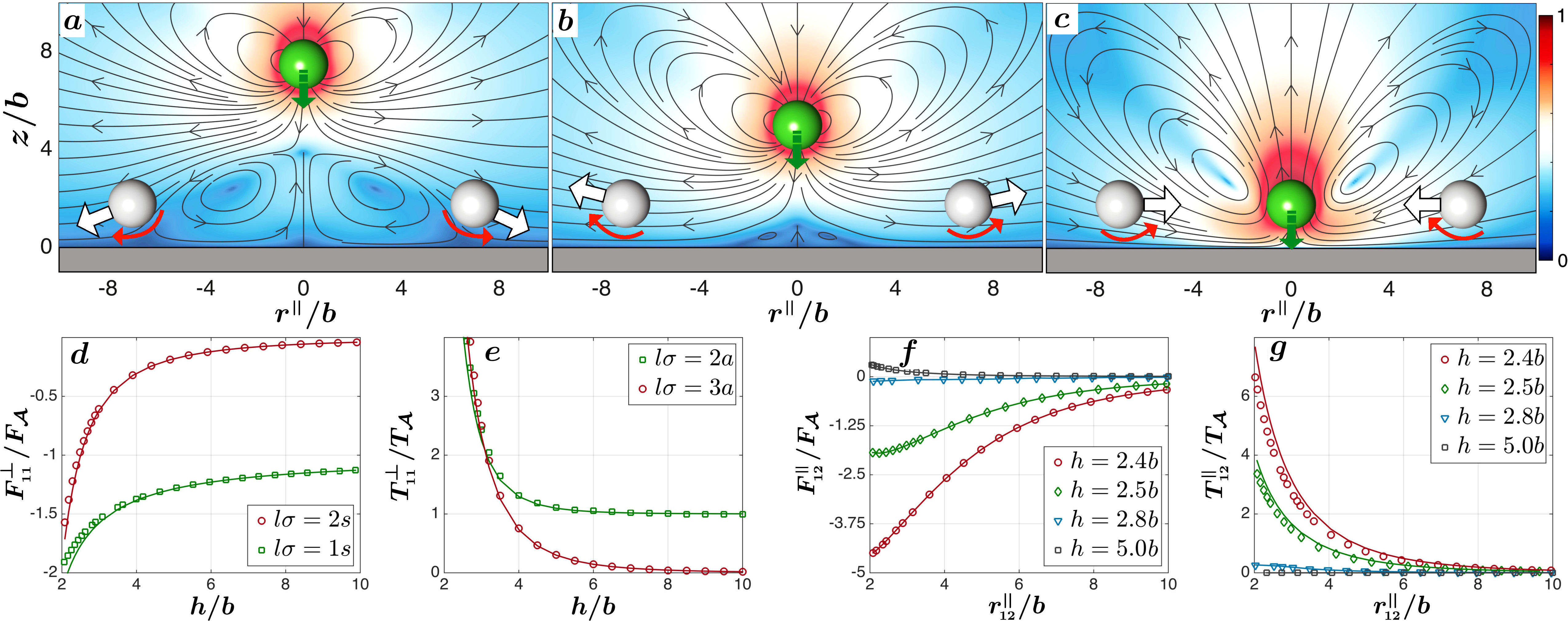
Figure 2: Distortion of the flow produced by leading polar $(l\sigma=1s)$ and apolar $(l\sigma=2s)$ slip terms in Eq.(2) as an active colloid of radius $b$, shown in green, approaches a plane wall. Tracer colloids are show in white. The streamlines of the fluid flow have been overlaid on the pseudocolor plot of logarithm of the magnitude of local flow normalised by its maximum. The flow in (c) results when the colloid is brought to rest near the wall. Hydrodynamic forces attract nearby colloids, as shown by the thick white arrows, leading to crystallization. Hydrodynamic torques tend to reorient the colloids as shown by the curved red arrows. The remaining graphs show quantitative variation of the active forces and torques from modes in Eq. (2) scaled by $F_{\mathcal{A}}=6\pi\eta bv_{s}$ and $T_{\mathcal{A}}=8\pi\eta b^{2}v_{s}$ respectively as a function of height $h$ of the colloid from the wall and distance, $\mathbf{r}_{ij}=\mathbf{R}_{i}-\mathbf{R}_{j}$, from other colloids . Solid and dotted lines represent analytical and numerical results respectively (see text). Here $\parallel$ and $\perp$ indicate directions parallel and perpendicular to the wall at $\mathbf{z}=0$.

Active forces and torques: Newton’s equations of motion for the colloids reduce, when inertia is negligible, to instantaneous balance of forces and torques

$$\mathbf{F}_{i}^{H}+\mathbf{F}_{i}^{P}+\boldsymbol{\xi}_{i}^{T}=0,\quad\mathbf{T}_{i}^{H}+\mathbf{T}_{i}^{P}+\boldsymbol{\xi}_{i}^{R}=0.$$ (3)

Here $\mathbf{F}_{i}^{H}=\int\mathbf{f}\,d\text{S}_{i}$, $\mathbf{F}^{P}$ and $\mathbf{\boldsymbol{\xi}^{T}}$ are respectively the hydrodynamic, body and Brownian forces while, $\mathbf{T}_{i}^{H}=\int\boldsymbol{\rho}_{i}\mathbf{\times}\mathbf{f}\,d\text{S}_{i}$, $\mathbf{T}_{i}^{P}$ and $\boldsymbol{\xi}_{i}^{R}$ are, corresponding torques, $\boldsymbol{\sigma}$ is the Cauchy stress in the fluid and $\mathbf{f}=\bm{\hat{\rho}_{i}}\cdot\boldsymbol{\sigma}$ is the traction. The linearity of the Stokes equation implies that these must be of the form

$$\mathbf{F}_{i}^{H}= -\boldsymbol{\gamma}_{ij}^{TT}\mathbf{\cdot V}_{j}-\boldsymbol{\gamma}_{ij}^{TR}\mathbf{\cdot\boldsymbol{\Omega}}_{j}-\sum_{l\sigma=1s}^{\infty}\boldsymbol{\gamma}_{ij}^{(T,\,l\sigma)}\negmedspace\cdot\mathbf{V}_{j}^{(l\sigma)},$$ (4a)

$$\mathbf{T}_{i}^{H}= -\boldsymbol{\gamma}_{ij}^{RT}\mathbf{\cdot V}_{j}-\boldsymbol{\gamma}_{ij}^{RR}\mathbf{\cdot\boldsymbol{\Omega}}_{j}-\sum_{l\sigma=1s}^{\infty}\boldsymbol{\gamma}_{ij}^{(R,\,l\sigma)}\negmedspace\cdot\mathbf{V}_{j}^{(l\sigma)},$$ (4b)

where repeated particle indices are summed over. The $\boldsymbol{\gamma}_{ij}^{\alpha\beta}$, with $\alpha,\beta=T,R$, are the usual friction matrices associated with rigid body motion and $\mathcal{\boldsymbol{\gamma}}_{ij}^{(\alpha,\,l\sigma)}$ are friction tensors associated with the irreducible modes of the active slip. They are of rank $l+1$, $l$, and $l-1$, respectively, for $\sigma=s,a,t$. The forces and torques depend on relative position (through the $\mathcal{\boldsymbol{\gamma}}_{ij}^{(\alpha,\,l\sigma)}$) and on relative orientation (through the $\mathbf{V}_{j}^{(l\sigma)}$). Their signature under time-reversal shows that the active contributions are dissipative.

We calculate the friction tensors using a Galerkin discretization of the boundary integral equation Singh et al. (2015); Singh and Adhikari (2016) with the Lorentz-Blake Green’s function Blake (1971) which, by construction, vanishes at the plane wall. The $\boldsymbol{\gamma}_{ij}^{(T,\,l\sigma)}$ decay as $r_{ij}^{-(l+1)}$ and $r_{ij}^{-(l+2)}$ in the directions parallel and perpendicular to the wall. The $\boldsymbol{\gamma}_{ij}^{(R,\,l\sigma)}$ decay one power of $r_{ij}$ more rapidly. While the force and torque so obtained are sufficient to study colloidal motion, additional insight is obtained from studying the flow, which we compute from its boundary integral representation. Further details are given in sup .

The modes $l\sigma=1s$ and $l\sigma=2a$ contribute most dominantly to forces and torques and they attain their lower bounds far away from the wall, where their magnitudes are ${\color[rgb]{0,0,0}F=6\pi\eta bv_{s}}$ and $T=8\pi\eta b^{3}\omega_{s}$. The bacteria in Petroff et al. (2015) have radius $b\sim 4\,\mu\text{m}$, swimming speed $v_{s}\sim 500\,\mu\text{m/s}$ and angular speed $\omega_{s}\sim 50\,s^{-1}$ in a fluid of viscosity $\eta=10^{-3}\,\text{kg/ms}$. This gives an estimate of $F\sim 40\times 10^{-12}\,\text{N}$ and$T\sim 10^{-16}$ Nm. For the synthetic colloids in Palacci et al. (2013), $b\sim 2\,\mu\text{m}$, $v_{s}\sim 10\,\mu\text{m/s}$, which corresponds to $F_{\mathcal{}}\sim 10^{-13}\,\text{N}$. Typical Brownian forces and torques are of order $\mathcal{O}\left(k_{B}\text{T/b}\right)\sim 10^{-15}\,\text{N}$, and $\mathcal{O}\left(k_{B}\text{T}\right)\sim 10^{-21}\,\text{Nm}$ respectively. Thus active forces and torques overwhelm Brownian contributions by factors of 100 or more in these experiments and, henceforth, we neglect their effects. Trajectories are obtained by integrating the kinematic equations $\mathbf{\dot{R}}_{i}=\mathbf{V}_{i}$ and $\dot{\mathbf{p}}_{i}=\mathbf{\Omega}_{i}\times\mathbf{p}_{i}$, where $\mathbf{V}_{i}$ and $\mathbf{\boldsymbol{\Omega}}_{i}$ satisfy Eq. (3) with Brownian contributions removed. Integration methods and parameter choices are detailed in sup .

Crystallization kinetics: The kinetics of crystallization obtained from numerical solutions is shown in Movie 1 sup , together with the evolution of the structure factor $S(\mathbf{k})$. The uniform state is destabilized, most notably for any initial density, by attractive active hydrodynamic forces. Steric repulsion between particles balances these to produce crystallites with hexagonal positional order. Rings in the structure factor first appear at wavenumbers that correspond to Bragg vectors of the lattice, reminiscent of a spinodal instability, representing the averaged scattering from randomly oriented crystallites. These sharpen into Bragg peaks as the crystallites coalesce and orientational order grows. Finally particles assemble into a single crystallite which continues to rotate, while the structure factor shows a clear sixfold symmetry. In Movie 2 sup we show the formation of a hexagonal unit cell from the simulation of seven polar and chiral active colloids. The crystallite rotates with an angular velocity parallel to the chiral axis of the colloids.

Universal mechanisms: To better understand the mechanisms behind active crystallization we show, in Fig. (2) , the active flow near a wall and the dominant contributions to the flow-mediated forces and torques. The top three panels show the increasing distortion of the flow produced by the leading polar $(l\sigma=1s)$ and apolar $(l\sigma=2s)$ modes for $\mathbf{p}_{i}$ normal to the wall and $V_{0}^{(2s)}<0.$ The flow develops a monopolar character as the colloid is brought to rest at a height $h$ by the balance of hydrodynamic attraction, Fig. (2d), and steric repulsion from the wall. The induced monopole on the colloids leads to attractive forces between them below a critical height $h$ from the wall as shown in Fig. (2f). Nearby colloids entrained in this flow are attracted towards the central colloid as shown in the rightmost panel and in Movie 3 sup . The balance of the hydrodynamic attraction and steric repulsion determines the lattice spacing $d$. We note that even an apolar colloid is attracted to the wall, Fig. (2d), and induces hydrodynamic attractive forces. Thus, unlike MIPS Cates and Tailleur (2015), polarity is not necessary for crystallization. The induced monopole also tends to reorient the colloids, by generating a torque in the plane of wall, as shown by the curved red arrows in Fig. (2c) and quantified in Fig. (2g). Their destabilizing effect can be nullified by external torques $\mathbf{T}_{i}^{P}=T_{0}(\mathbf{\hat{z}}\times\mathbf{p}_{i})$ in the plane of the wall due, for example, to bottom-heaviness. The orientation can also be stabilized by the chiral terms in Eq. (2), which produce torques $\perp$ to the wall, as shown in Fig. (2e). This chiral torque acting $\perp$ to the wall, when combined with destabilizing torque $\parallel$ to the wall, induces active precession of the orientation about the wall normal, thereby stabilizing the orientations. The role of each of the six terms in Eq. (2) in generating positional order, orientational order and crystal rotation is tabulated in sup . Activity and body forces pointing away from the wall are necessary for positional order while bottom-heaviness or chirality is necessary for orientational stability.

Harmonic excitations: We now study harmonic excitations $\mathbf{u}_{i}$ of a perfect hexagonal crystal by expanding the positions as $\mathbf{R}_{i}=\mathbf{R}_{i}^{0}+\mathbf{u}_{i}$ around the stationary state $\mathbf{R}_{i}^{0}=(X_{i}^{0},\,Y_{i}^{0},\,h)$ and ignoring orientational fluctuations. Force balance to leading order gives

$$-\boldsymbol{\gamma}_{ij}^{TT}\cdot\dot{\mathbf{u}}_{j} +\left(\mathbf{\boldsymbol{\nabla}}_{j}\boldsymbol{\gamma}_{ij}^{TT}\cdot\mathbf{V}^{\mathcal{A}}-\mathbf{D}_{ij}\right)\cdot\mathbf{u}_{j}=0,$$ (5)

where $\mathbf{D}_{ij}=-\boldsymbol{\nabla}_{j}\boldsymbol{\nabla}{}_{i}U\big{|}_{0}$ and $U$ is the sum of all steric potentials. This shows that relaxation is determined by both activity and elasticity, unlike in an equilibrium colloidal crystal where elasticity alone relaxes strains. The normal modes of relaxation can be obtained by Fourier transforming in the plane and in time. The dispersion is found from the solutions of

$$\det\Big{|}-i\omega\boldsymbol{\gamma}_{\mathbf{k}}^{TT}+i\mathbf{k}\,\boldsymbol{\gamma}_{\mathbf{k}}^{TT}\cdot\mathbf{V}^{\mathcal{A}}-\mathbf{D}_{\mathbf{k}}\Big{|}=0.$$ (6)

Here $\mathbf{k}=(k_{1},\,k_{2})$ is the wavevector restricted to the first Brillouin zone sup , $\omega$ is the frequency and $\mathbf{D}_{\mathbf{k}}$ is the dynamical matrix. The pair of dispersion relations for motion parallel to the wall are shown in Fig. (3). The dispersion for $k\ll k_{0}$, where $k_{0}$ is the magnitude of the reciprocal lattice vector, is quadratic in wavenumber

$$\omega_{\pm}=-i\tfrac{\gamma_{\perp}^{T}hv_{s}}{2\gamma_{{\mkern 3.0mu\vphantom{\perp}\vrule depth=0.0pt\mkern 2.5mu\vrule depth=0.0pt\mkern 3.0mu}}^{T}}f_{\pm}(\theta)\,k^{2},$$ (7)

where $f_{\pm}(\theta)$ are angular factors, $\gamma_{{\mkern 3.0mu\vphantom{\perp}\vrule depth=0.0pt\mkern 2.5mu\vrule depth=0.0pt\mkern 3.0mu}}^{T}$ and $\gamma_{\perp}^{T}$ are one-body frictions parallel and perpendicular to the wall, and $\tan\theta=\tfrac{k_{2}}{k_{1}}$. The small-$k$ approximation is compared with the numerical solution in Fig. (3) and it is found to hold for $k\lesssim 0.1k_{0}$. These can be interpreted as overdamped phonon modes of the active crystal joa . The presence of the active term $i\mathbf{k}\,\boldsymbol{\gamma}_{\mathbf{k}}^{TT}\cdot\mathbf{V}^{\mathcal{A}}$ in Eq. (6) makes them differ from phonon modes of a colloidal crystal.

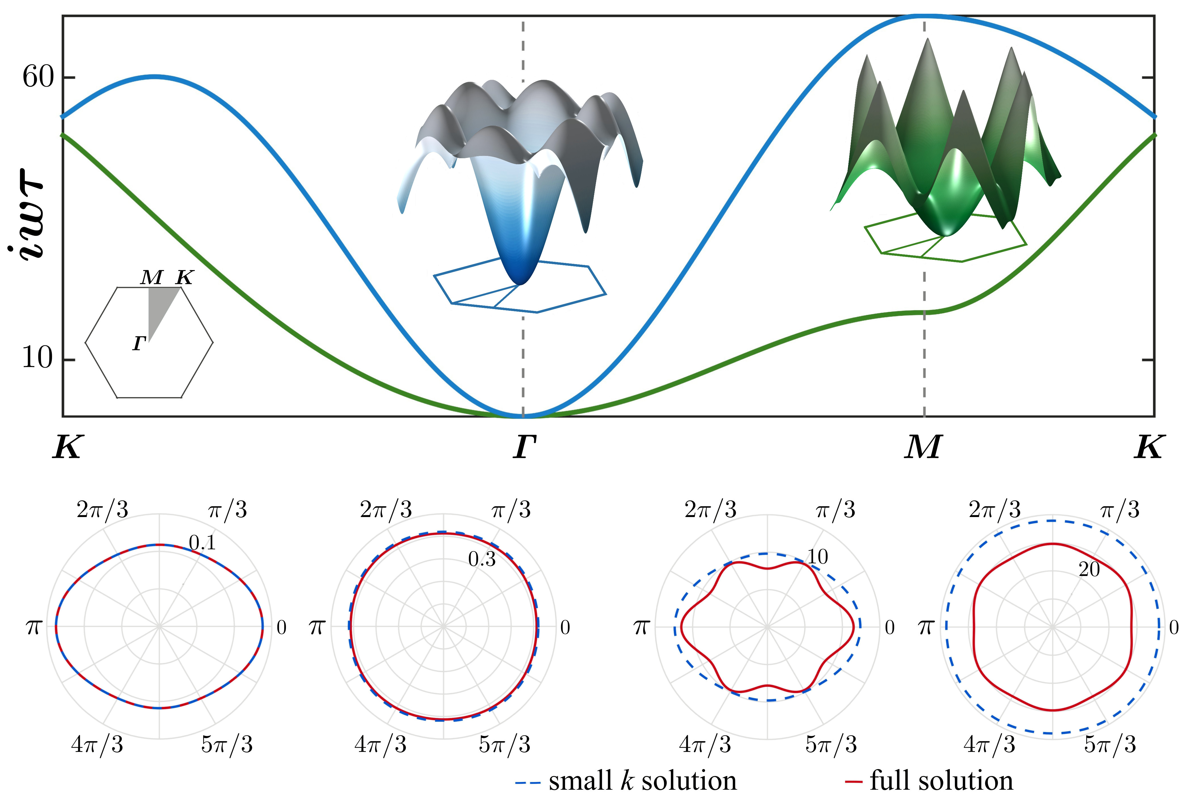
Figure 3: Branches of the dispersion relation for the two planar normal modes of relaxation of a hexagonal active crystal. The curves in upper panel show the dispersion along high symmetry directions of the Brillouin zone (first inset). The surfaces in the second and third insets show the dispersion over the entire Brillouin zone. Polar plots in the lower panel, have comparisons of full numerical solution of Eq. (6) with the approximate solution at small $k$ of Eq. (7) for $k=0.01k_{0}$ (left panel) and $k=0.3k_{0}$ (right panel).

Discussion: In this work, we have considered only hydrodynamic forces and torques, unlike the case of MIPS Tailleur and Cates (2008); Cates et al. (2010); Cates and Tailleur (2013, 2015) where Brownian torques drives reorientations Henkes et al. (2011); Fily and Marchetti (2012); Bialké et al. (2012); Redner et al. (2013). We have shown that the latter are at least two orders of magnitude weaker than the former for experiments in the class of Palacci et al. (2013); Petroff et al. (2015). However, it is conceivable that thermal fluctuations will play a more significant role when the activity is comparatively weak, modifying both the nature of crystallization transition and the stability of the crystalline phase. The spinodal-like instability appears due to the uncompensated long-ranged attractive active forces. These can be compensated by entropic forces to stabilize the disordered phase at finite temperatures. A nucleational route to crystallization, with activity-enhanced rates, is then possible in the regime where the active forces reduce the nucleation barrier without driving it to zero. In the crystalline phase, thermal fluctuations will excite both phonon and topological modes. Phonon fluctuations will destroy long-range translational order Peierls (1935); Landau (1937), but due to the activity-enhanced stiffness of these modes, large system sizes (compared to equilibrium) will be needed to observe the power-law decay of correlations. Topological defects will be excited at higher temperatures and a defect unbinding transition Kosterlitz and Thouless (1973); Halperin and Nelson (1978); Nelson and Halperin (1979); Young (1979); Chaikin and Lubensky (2000), modified by activity, may destroy translational order entirely, producing instead an “active” hexatic phase. These present exciting avenues for future research. We remark that wall-bounded clustering phenomena in algae Drescher et al. (2009) and charged colloids Squires (2001) are mediated by specific forms of the universal hydrodynamic mechanisms presented here.

Finally, we suggest that the flow-induced phase separation found here may provide a paradigm, complementary to MIPS, in which theoretical and experimental studies of momentum-conserving driven Yeo et al. (2015) and active matter Trau et al. (1996); Solomentsev et al. (1997); Matas-Navarro et al. (2014); Pandey et al. (2016); Wang et al. (2015); Wykes et al. (2016) may be situated.

We thank M. E. Cates, P. Chaikin, D. Frenkel, D. J. Pine, A. Laskar and T. V. Ramakrishnan for helpful discussions and IMSc for computing resources on the Nandadevi clusters.

Supplemental information

Appendix A Active force, torque and flow

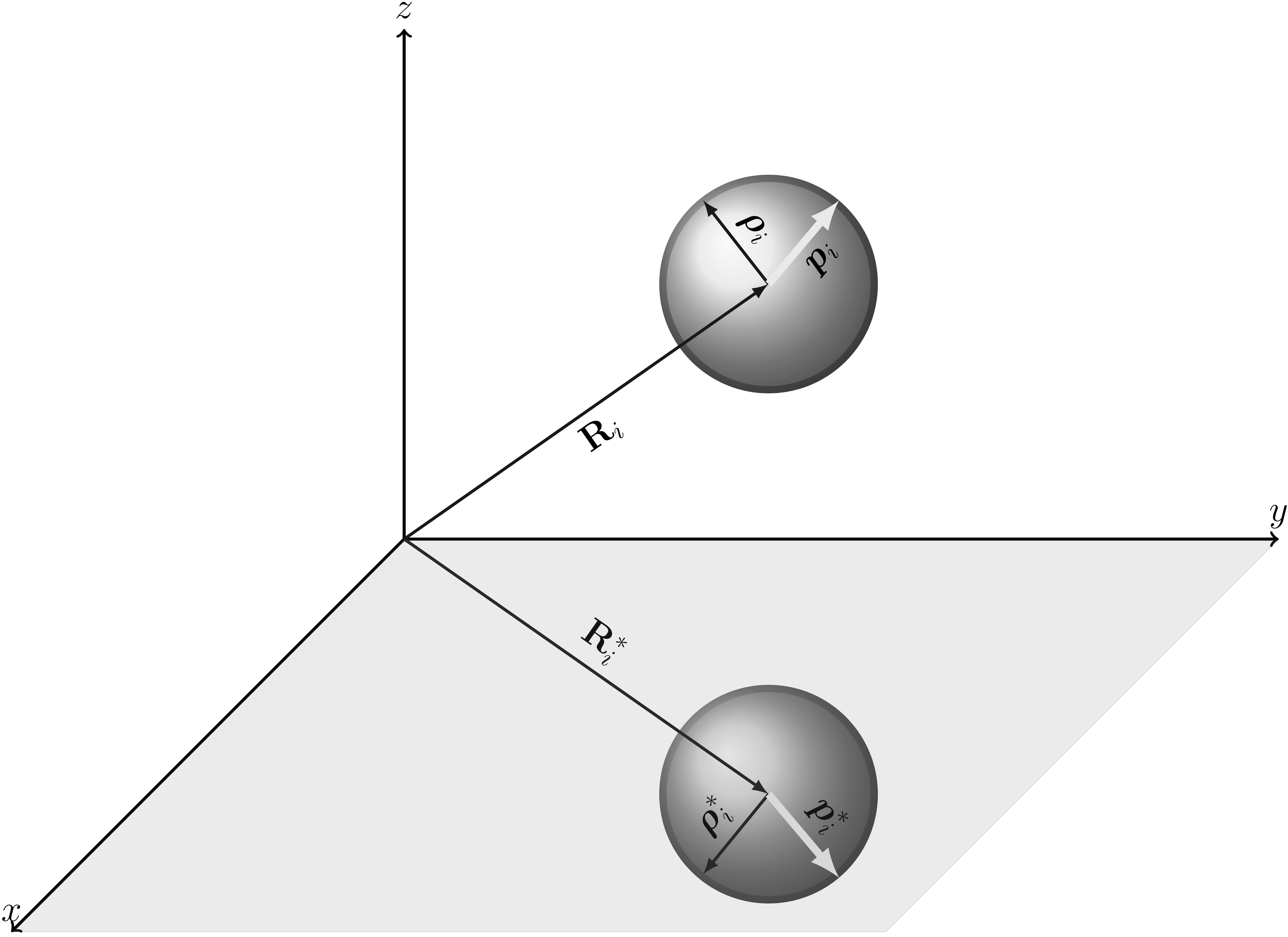
Figure 4: Coordinate system used to describe active spherical particles and its images near a no-slip wall. The $i$-th particle and its image is shown. See text for description.

We derive, in this section, the expressions for the active forces, torques, and exterior flow in a suspension of $N$ active colloids bounded by a plane wall. The system of coordinates is shown in Fig. (4). The spheres are centered at $\mathbf{R}_{i}$ and their velocities and angular velocities are $\mathbf{V}_{i}$ and $\mathbf{\Omega}_{i}$ respectively. ${\bf p}_{i}$ denotes the orientation of the particle while points on the boundaries of the spheres is given by $\mathbf{s}_{i}=\mathbf{R}_{i}+\boldsymbol{\rho}_{i}$, where $\boldsymbol{\rho}_{i}$ is the radius vector. To ensure no-slip on the wall, we associate am image centered at ${\bf R}_{i}^{*}$ with the $i$-th colloid Blake (1971), and a similar correspondence for all other quantities of the colloid and its image.

We closely follows our previous work Singh et al. (2015); Singh and Adhikari (2016) where a boundary integral formulation has been used to solve the Stokes equation with arbitrary boundary conditions. The principal difference here is in the choice of the Green’s function which satisfies the no-slip condition at the plane wall Blake (1971). In the interest of being self-contained, we repeat certain key steps en route to the solution. A clear expression of the linearity of Stokes flow is found in its integral representation, where the flow in the bulk is given in terms of integrals of the tractions and velocities at the boundaries Odqvist (1930); Ladyzhenskaia (1969); Pozrikidis (1992); Kim and Karrila (1992),

$$v_{\alpha}(\mathbf{r})= -\int G_{\alpha\beta}^{W}(\mathbf{r},\,\mathbf{s}_{j})f_{\beta}(\mathbf{s}_{j})\,d\mathrm{S}_{i}$$

$$+ \int K_{\beta\alpha\gamma}^{W}(\mathbf{r},\,\mathbf{s}_{j})\hat{\rho}_{\gamma}v_{\beta}(\mathbf{s}_{j})\,d\mathrm{S}_{i},$$ (8)

where repeated particle indices are summed over, $\mathbf{s}_{j}=\mathbf{R}_{j}+\boldsymbol{\rho}_{j}$ is a point on the surface of $j$-th particle and $G_{\alpha\beta}^{W}(\mathbf{r},\,\mathbf{s}_{j})$ is the Green’s function of the Stokes system satisfying no-slip condition, $\mathbf{v}=0$ on the wall at $z=0$. The stress tensor $K_{\alpha\beta\gamma}^{W}(\mathbf{r},\,\mathbf{s}_{j})$ and the pressure vector $P_{\alpha}^{W}$($\mathbf{r},\,\mathbf{s}_{j})$ satisfy $K_{\alpha\beta\gamma}^{W}(\mathbf{r},\,\mathbf{s}_{j})=-\delta_{\alpha\gamma}P_{\beta}^{W}+\eta\left(\nabla_{\gamma}G_{\alpha\beta}^{W}+\nabla_{\alpha}G_{\beta\gamma}^{W}\right)$ and $-\nabla_{\alpha}P_{\beta}^{W}(\mathbf{r},\mathbf{r^{\prime}})+\eta\nabla^{2}G_{\alpha\beta}^{W}=-\delta\left(\mathbf{r}-\mathbf{r^{\prime}}\right)\delta_{ij}$ respectively.

We solve the Fredholm integral equation of Eq. (8) by expanding the boundary fields in irreducible tensorial spherical harmonics, $\mathbf{Y}^{(l)}$, which are orthogonal basis function on the surface of the sphere $\frac{1}{4\pi b^{2}}\int\mathbf{Y}^{(l)}(\widehat{\bm{\rho}})\,\mathbf{Y}^{(l^{\prime})}(\widehat{\bm{\rho}})\,d\mathrm{S}=\delta_{ll^{\prime}}\,\frac{l!\,(2l-1)!!}{(2l+1)}\mathbf{\Delta}^{(l)},$ where $\mathbf{\Delta}^{(l)}$ is tensor of rank $2l$, projecting any $l$-th order tensor to its symmetric irreducible form Mazur and Saarloos (1982); Hess and Köhler (1980). The boundary velocity including active slip and its expansion in this basis has been provided above. The orthogonality of the basis functions gives the expansion coefficients in terms of surface integrals of traction and velocity as Ladd (1988); Ghose and Adhikari (2014),

$$\mathbf{F}_{i}^{(l)} =\frac{1}{(l-1)!(2l-3)!!}\int\mathbf{f}(\mathbf{R}_{i}+\bm{\rho}_{i})\mathbf{Y}^{(l-1)}(\bm{\hat{\rho}}_{i})\,d\mathrm{S}_{i},$$

$$\mathbf{V}_{i}^{(l)} =\frac{2l-1}{4\pi b^{2}}\int\mathbf{v}^{\mathcal{A}}(\mathbf{R}_{i}+\bm{\rho}_{i})\mathbf{Y}^{(l-1)}(\bm{\hat{\rho}}_{i})\,d\mathrm{S}_{i}.$$ (9)

The coefficients of the traction and velocity are tensors of rank $l$ and can be written as irreducible tensor of rank $l,$ $l-1$ and $l-2$ Singh et al. (2015). The first term in the traction expansion is the force $\mathbf{F}_{i}^{(1)}=\mathbf{F}_{i}^{H}$, while the antisymmetric part of the second term is the torque $b\boldsymbol{\varepsilon}\cdot\mathbf{F}_{i}^{(2)}=\mathbf{T}_{i}^{H}$. The first term in the velocity expansion is $\mathbf{V}_{i}^{(1)}=-\mathbf{V}_{i}^{\mathcal{A}}$ and the antisymmetric part of the second term is $\tfrac{1}{2b}\boldsymbol{\boldsymbol{\varepsilon}}\cdot\mathbf{V}_{i}^{(2)}=-\mathbf{\Omega}_{i}^{\mathcal{A}}$. Here $\mathbf{V}_{i}^{\mathcal{A}}=-\tfrac{1}{4\pi b^{2}}\int\mathbf{v}^{\mathcal{A}}(\bm{\rho}_{i})\,d\mathrm{S}_{i}$ denotes the self-propulsion, while $\bm{\Omega}_{i}^{\mathcal{A}}=-\frac{3}{8\pi b^{4}}\int\bm{\rho}_{i}\times\mathbf{v}^{\mathcal{A}}(\bm{\rho}_{i})\,d\mathrm{S}_{i}$ denotes the self-rotation of an isolated active colloid in unbounded flow. The expression for fluid flow can be obtained in terms of coefficients of traction and velocity,

$$\mathbf{v}(\mathbf{r})=\sum_{l=1}^{\infty}\Big{(}-\boldsymbol{G}_{j}^{(l)}\cdot\mathbf{F}_{j}^{(l)}+ \boldsymbol{K}_{j}^{(l)}\cdot\mathbf{V}_{j}^{(l)}\Big{)},$$ (10)

where the boundary integrals $\boldsymbol{G}_{j}^{(l)}$ and $\boldsymbol{K}_{j}^{(l)}$ can be written in terms of Green’s function and its derivatives (Appendix E). We multiply the fluid velocity by the $l$-th tensorial harmonic and integrate over the $i$-th boundary. Using the orthogonality of these basis functions, we obtain an infinite-dimensional linear system of equations for the unknown traction coefficients Singh et al. (2015),

$$\tfrac{1}{2}\,\mathbf{V}_{i}^{(l)}=\sum_{l^{\prime}=1}^{\infty}\Big{(}-\boldsymbol{G}_{ij}^{(l,\,l^{\prime})}\cdot\mathbf{F}_{j}^{(l^{\prime})} +\boldsymbol{K}_{ij}^{(l,\,l^{\prime})}\cdot\mathbf{V}_{j}^{(l^{\prime})}\Big{)},$$ (11)

where the matrix elements $\boldsymbol{G}_{ij}^{(l,\,l^{\prime})}$ and $\boldsymbol{K}_{ij}^{(l,\,l^{\prime})}$ can be evaluated in terms of the Green’s function and its derivatives, as given in Appendix E.

The traction and velocity coefficients are reducible and their irreducible decomposition is given as Brunn (1976); Schmitz (1980),

$$\mathbf{F}_{i}^{(ls)}=\overbracket{\mathbf{F}_{i}^{(l)}},\quad \mathbf{F}_{i}^{(la)}=\overbracket{\bm{\varepsilon}\cdot\mathbf{F}_{i}^{(l)}},\quad \mathbf{F}_{i}^{(lt)}={\bm{\delta}\cdot\mathbf{F}_{i}^{(l)}},$$

$$\mathbf{V}_{i}^{(ls)}=\overbracket{\mathbf{V}_{i}^{(l)}},\quad \mathbf{V}_{i}^{(la)}=\overbracket{\boldsymbol{\mathbf{\varepsilon}}\cdot\mathbf{V}_{i}^{(l)}},\quad \mathbf{V}_{i}^{(lt)}={\bm{\delta}\cdot\mathbf{V}_{i}^{(l)}}.$$

Here the operator $\overbracket{(\dots)}=\boldsymbol{\Delta}^{(l)}(\dots)$ extracts the symmetric irreducible part of the tensor it acts on. We use these irreducible coefficients and the linear system of equations to solve for the unknown traction in terms of the known boundary velocity Singh and Adhikari (2016). The relations between the irreducible coefficients of the traction and velocity, then, becomes Singh and Adhikari (2016),

$$\mathbf{F}_{i}^{(l\sigma)}= -\boldsymbol{\gamma}_{ij}^{(l\sigma,\,1s)}\cdot\mathbf{V}_{j}-\boldsymbol{\gamma}_{ij}^{(l\sigma,\,R)}\cdot\mathbf{\Omega}_{j}$$

$$- \sum_{l^{\prime}\sigma^{\prime}=1s}^{\infty}\boldsymbol{\gamma}_{ij}^{(l\sigma,\,l^{\prime}\sigma^{\prime})}\cdot\mathbf{V}_{j}^{(l^{\prime}\sigma^{\prime})}.$$ (12)

This infinite set of equations, called the traction laws Singh and Adhikari (2016), manifestly shows the linear relation between the traction and velocity coefficients and defines the friction tensors. The expressions for the friction tensors can be obtained by an iterative scheme Singh and Adhikari (2016). We use the one-body solution as the initial guess for the iteration,

$$\mathbf{F}_{i}^{H}=-\gamma^{T}(\mathbf{V}_{i}-\mathbf{V}_{i}^{\mathcal{A}}),\qquad\mathbf{T}_{i}^{H}=-\gamma^{R}(\mathbf{\Omega}_{i}-\mathbf{\Omega}_{i}^{\mathcal{A}}),$$ (13)

where $\gamma^{T}$ and $\gamma^{R}$ are one particle friction corresponding to translation and rotation. Near a wall no-slip wall, they are, ${\gamma}^{T}=\gamma_{\perp}^{T}\hat{\boldsymbol{z}}+\gamma_{{\mkern 3.0mu\vphantom{\perp}\vrule depth=0.0pt\mkern 2.5mu\vrule depth=0.0pt\mkern 3.0mu}}^{T}(\hat{\boldsymbol{x}}+\hat{\boldsymbol{y}})$ and ${\gamma}^{R}=\gamma_{\perp}^{R}\hat{\boldsymbol{z}}+\gamma_{{\mkern 3.0mu\vphantom{\perp}\vrule depth=0.0pt\mkern 2.5mu\vrule depth=0.0pt\mkern 3.0mu}}^{R}(\hat{\boldsymbol{x}}+\hat{\boldsymbol{y}})$ Kim and Karrila (1992). Here       and $\perp$ subscripts indicating directions parallel and perpendicular to the wall. The expressions after one iteration, corresponding to the “first reflection” in Smoluchowski’s classical method, are shown in Appendix F.

Appendix B Crystalline steady states

In this section we work out the steady states of the active crystals using the leading terms of the force and torque equations. Using the leading order force balance for $i$-th particle, the steady state condition for position is given as

$$\bm{\gamma}_{ij}^{TT}\cdot\mathbf{V}_{j}^{\mathcal{A}}+\mathbf{F}_{i}^{P}=0.$$ (14)

Here $\mathbf{V}_{i}^{\mathcal{A}}=-v_{s}\hat{\mathbf{z}}$ is self-propulsion of the colloid at a speed $v_{s}$, assumed to be moving $\perp$ to the wall. The body force $\mathbf{F}_{i}^{P}=-\boldsymbol{\nabla}_{{\scriptscriptstyle\mathbf{R}_{i}}}U$ is due to a short-ranged repulsive potential $U,$ which depends on displacement $\mathbf{r}_{ij}=\mathbf{R}_{i}-\mathbf{R}_{j}$ and is given as, $U(r_{ij})=\epsilon\left(\frac{r_{min}}{r_{ij}}\right)^{12}-2\epsilon\left(\frac{r_{min}}{r_{ij}}\right)^{6}+\epsilon,$ for $r_{ij}<r_{min}$ and zero otherwise Weeks et al. (1971), where $\epsilon$ is the potential strength. The same potential has been used to model colloid-colloid repulsion $\mathbf{F}_{i}^{PP}$ and the colloid-wall repulsive force $\mathbf{F}_{i}^{PW}$.

One- and two-body dynamics: To estimate the height at which the particle is brought to rest close to the wall, we use the $z-$component of the force balance, $-\gamma_{\perp}^{T}v_{s}=F_{3}^{PW}$. Here $F_{3}^{PW}$ is the repulsive force from the wall in $\mathbf{\hat{z}}$ direction, while $\gamma_{\perp}^{T}v_{s}$ is the attractive force of the colloid to the wall in same direction. The balance between the attraction and repulsion sets the height $h$ at which the colloid is brought to rest. We now consider force balance for a pair of particles in planar direction,

$$-v_{s}\gamma_{{\mkern 3.0mu\vphantom{\perp}\vrule depth=0.0pt\mkern 2.5mu\vrule depth=0.0pt\mkern 3.0mu}}^{T}\gamma_{\perp}^{T}\mbox{$\mathcal{F}$}_{i}^{0}\mbox{$\mathcal{F}$}_{j}^{0}G_{\alpha 3}^{W}(\mathbf{R}_{i},\mathbf{R}_{j})+F_{\alpha}^{PP} =0,$$ (15)

where

$$\mathcal{F}_{i}^{l}=\left(1+\tfrac{b^{2}}{4l+6}\boldsymbol{\nabla}_{{\scriptscriptstyle\mathbf{R}_{i}}}^{2}\right),$$ (16)

is an operator encoding the finite size of the sphere and $\alpha$ may takes either of the values 1 or 2 corresponding to two equivalent directions parallel to wall. We have used results provided in Appendix F, to write the expression for friction. The solution of this equation gives the lattice spacing $d$. For fixed particle-wall potential, increasing $v_{s}$ decreases the resting height $h$ and separation between pairs, $d$, as show in Fig. (5).

Rotational dynamics: In Fig. (1), we show the state diagram, obtained from simulation, which shows that the crystal is stable over a critical strengths of either bottom-heaviness or chirality. For an initially symmetric distribution, a crystal stabilized by external torque alone does not rotate, while the crystal stabilized by chirality does rotate. When the crystal is rotating at an angular velocity $\mathbf{\Omega}_{c}$ about its center of mass $\mathbf{R}_{c}$, the velocity the $i$-th colloid at position $\mathbf{R}_{i}$ can be then written as $\mathbf{\dot{R}}_{i}=\mathbf{\Omega}_{c}\times\mathbf{R}_{i}$. Force balance parallel to the wall is then

$$\bm{\gamma}_{ij}^{TT}\cdot\left[\mathbf{\Omega}_{c}\times(\mathbf{R}_{j}-\mathbf{R}_{0}^{c})\right]+\bm{\gamma}_{ij}^{TR}\cdot\mathbf{\Omega}_{j}=0.$$ (17)

The angular speed perpendicular to wall is $\Omega=\Omega_{i}^{\mathcal{A}}$. This implies that in absence of chiral self-rotation there is no rotation of the crystal. The angular velocity of the crystal can be obtained by power counting - $\bm{\gamma}_{ij}^{TT}$ scales as $r_{ij}^{-3}$ in direction parallel to wall while $\bm{\gamma}_{ij}^{TR}$ scales as $r_{ij}^{-4}$. The angular velocity of the crystal, then, scales as $\Omega_{c}\propto 1/R_{c}^{2}$. In Fig. (1) we show that rotation period of a crystal scales inversely as number of particles $N$ in the crystal for an assembly of chiral particles, which is an excellent agreement with a recent experiment Petroff et al. (2015).

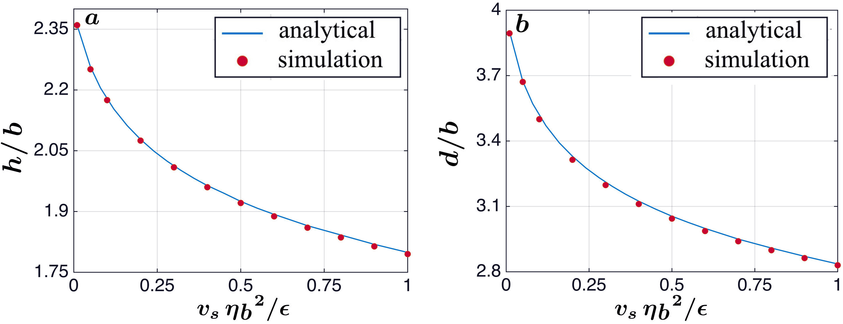
Figure 5: Steady states of active crystallization. Left panel has the plot of leading terms for the analytical solution of height $h$, shown in solid line, along with the full numerical result, shown as dotted curve. Right panel has similar set of plots for lattice spacing $d$. The leading order estimates are found to be in agreement with the numerical solution.

Appendix C Harmonic excitations

In this section we study harmonic excitations $\mathbf{u}_{i}$ of the crystal about a stationary state $\mathbf{R}_{i}^{0}=(X_{i}^{0},\,Y_{i}^{0},\,h)$, such that $\dot{\mathbf{R}}_{i}^{0}=0$ and $\mathbf{\Omega}_{i}^{0}=0$ at this location. The force balance condition is then $\boldsymbol{\gamma}_{ij}^{TT}\cdot\mathbf{V}_{j}^{\mathcal{A}}\big{|}_{0}+\mathbf{F}_{i}^{P}\big{|}_{0}=0$. We, now, consider a small displacement about this state $\mathbf{R}_{i}=\mathbf{R}_{i}^{0}+\mathbf{u}_{i}$. Expanding the friction tensors about the stationarity point, we have,

$$\boldsymbol{\gamma}_{ij}^{TT}=\boldsymbol{\gamma}_{ij}^{TT}\big{|}_{0}+(\mathbf{u}_{i}\cdot\mathbf{\boldsymbol{\nabla}}_{{\scriptscriptstyle\mathbf{R}_{i}}}-\mathbf{u}_{j}\cdot\mathbf{\boldsymbol{\nabla}}_{{\scriptscriptstyle\mathbf{R}_{j}}})\mathbf{}\boldsymbol{\gamma}_{ij}^{TT}\big{|}_{0}+\mathcal{O}(\mathbf{u}^{2}).$$

The force can be expanded in a similar way $\mathbf{F}_{i}^{P}=\mathbf{F}_{i}^{P}\big{|}_{0}-\mathbf{D}_{ij}\cdot\mathbf{u}_{j},$ where $\mathbf{D}_{ij}=-\boldsymbol{\nabla}_{{\scriptscriptstyle\mathbf{R}_{j}}}\mathbf{\boldsymbol{\nabla}}_{{\scriptscriptstyle\mathbf{R}_{i}}}U\big{|}_{0}$. Using the equations of motion and considering terms linear in the displacement, the equation becomes

$$-\boldsymbol{\gamma}_{ij}^{TT}\cdot\dot{\mathbf{u}}_{j} +\left(\mathbf{\boldsymbol{\nabla}}_{{\scriptscriptstyle\mathbf{R}_{j}}}\boldsymbol{\gamma}_{ij}^{TT}\cdot\mathbf{V}^{\mathcal{A}}-\mathbf{D}_{ij}\right)\cdot\mathbf{u}_{j}=0.$$

We seek a solution of the form $\mathbf{u}_{i}(t)=\mathbf{u}_{\mathbf{k}}(t)\,e^{i\mathbf{k}\cdot\mathbf{R}_{i}}.$ Using this, the force balance condition becomes,

$$-\boldsymbol{\gamma}_{\mathbf{k}}^{TT}\cdot\dot{\mathbf{u}}_{k}+\left(i\mathbf{k}\,\boldsymbol{\gamma}_{\mathbf{k}}^{TT}\cdot\mathbf{V}^{\mathcal{A}}-\mathbf{D}_{\mathbf{k}}\right)\cdot\mathbf{u}_{\mathbf{k}}=0.$$ (18)

Here $\mathbf{D}_{\mathbf{k}}$ is the Fourier transform of $\mathbf{D}_{ij}$ and $\boldsymbol{\gamma}_{\mathbf{k}}^{TT}$ is the Fourier transform of the friction tensor

$$\mathbf{D}_{\mathbf{k}} =\sum_{i=1}^{N}\mathbf{D}_{i1}\,e^{i\mathbf{k}\cdot(\mathbf{R}_{i}-\mathbf{R}_{1})},$$

$$\boldsymbol{\gamma}_{\mathbf{k}}^{TT} =\sum_{i=1}^{N}\boldsymbol{\gamma}_{i1}^{TT}\,e^{i\mathbf{k}\cdot(\mathbf{R}_{i}-\mathbf{R}_{1})}.$$

Here, $\mathbf{D}_{\mathbf{k}}$ is called the dynamical matrix Born and Huang (1954). We now write $\boldsymbol{\gamma}_{i1}^{TT}$ in terms of its planar Fourier transform

$$\boldsymbol{\gamma}_{i1}^{TT}=\int\hat{\boldsymbol{\gamma}}_{\mathbf{k}}^{TT}(\mathbf{k};\,h)e^{-i\mathbf{k}^{\prime}\cdot(\mathbf{R}_{i}-\mathbf{R}_{1})}\,\frac{d^{2}k^{\prime}}{(2\pi)^{2}},$$

to obtain an expression for $\boldsymbol{\gamma}_{\mathbf{k}}^{TT}$,

$$\boldsymbol{\gamma}_{\mathbf{k}}^{TT}(\mathbf{k};\,h) = \sum_{i}\int\hat{\boldsymbol{\gamma}}_{\mathbf{k}}^{TT}(\mathbf{k};\,h)e^{-i(\mathbf{k}^{\prime}-k)\cdot(\mathbf{R}_{i}-\mathbf{R}_{1})}\,\frac{d^{2}k^{\prime}}{(2\pi)^{2}},$$ (19)

$$= \frac{1}{A_{c}}\sum_{\lambda}\hat{\boldsymbol{\gamma}}_{\mathbf{k}}^{TT}(\mathbf{k}+\mathbf{q}_{\lambda};\,h).$$

Here we have used the identity

$$\sum_{i}e^{-i\mathbf{k}\cdot\mathbf{R}_{i}}=\frac{(2\pi)^{2}}{A_{c}}\sum\mathbf{\boldsymbol{\delta}}(\mathbf{k}-\mathbf{q}_{\lambda}),$$ (20)

where $A_{c}$ is area of the unit cell and $\mathbf{q}_{\lambda}$ are reciprocal lattice vectors. We now identify two parts of $\boldsymbol{\gamma}_{\mathbf{k}}^{TT},$

$$\boldsymbol{\gamma}_{\mathbf{k}}^{TT}(\mathbf{k};\,h)=\hat{\boldsymbol{\gamma}}_{{\scriptscriptstyle\mathbf{k}_{0}}}^{TT}(\mathbf{k};\,h)+\sum_{\lambda^{\prime}}\hat{\boldsymbol{\gamma}}_{{\scriptscriptstyle\mathbf{k}_{q}}}^{TT}(\mathbf{k}+\mathbf{q}_{\lambda};\,h)$$

Here $\hat{\boldsymbol{\gamma}}_{{\scriptscriptstyle\mathbf{k}_{0}}}^{TT}(\mathbf{k};\,h)$ corresponds to the $\mathbf{q}_{\lambda}=0$ and terms at arbitrary non-zero $q$ are denoted by $\hat{\boldsymbol{\gamma}}_{{\scriptscriptstyle\mathbf{k}_{q}}}^{TT}(\mathbf{k};\,h)$. Their leading order forms can be written as

$$\hat{\boldsymbol{\gamma}}_{{\scriptscriptstyle\mathbf{k}_{0}}}^{TT}(\mathbf{k};\,h) =\gamma^{T}\mathbf{I}+\frac{\gamma^{T}\gamma^{T}}{A_{c}}\mathcal{F}^{k}\,\hat{\mathbf{G}}^{W}(\mathbf{k};\,h),$$

$$\hat{\boldsymbol{\gamma}}_{{\scriptscriptstyle\mathbf{k}_{q}}}^{TT}(\mathbf{k};\,h) =\frac{\gamma^{T}\gamma^{T}}{A_{c}}\mathcal{F}^{k}\,\sum_{\lambda^{\prime}}\hat{\mathbf{G}}^{W}(\mathbf{k}+\mathbf{q}_{\lambda};\,h).$$

Here $\mathcal{F}^{k}=1-b^{2}k^{2}/3$ and $\hat{\mathbf{G}}^{W}(\mathbf{k};\,h)$ is the two-dimensional Fourier transform of $\mathbf{G}^{W}$ (see Appendix G). The prime on the summation on the right indicates that $\lambda=0$ is excluded from the sum. We now turn to the calculation of the dynamical matrix,

$$\mathbf{D}_{\mathbf{k}} =\sum_{i=1}^{N}\left(\frac{\mathbf{I}}{r^{2}}U^{\prime}+\frac{\mathbf{r}\,\mathbf{r}}{r^{4}}U^{\prime\prime}\right)_{0}\left(1-e^{i\mathbf{k}\cdot\mathbf{R}_{i}}\right).$$

Here $U^{\prime}=-12\epsilon\,\big{[}\left(r_{min}/d\right)^{12}-\left(r_{min}/d\right)^{6}\big{]}$ and $U^{\prime\prime}=12\epsilon\,\big{[}14\left(r_{min}/d\right)^{12}-8\left(r_{min}/d\right)^{6}\big{]}$. We evaluate the above in the nearest neighbor approximation in the direction parallel to the wall. The expression for $\mathbf{D}_{\mathbf{k}}$ and $\boldsymbol{\gamma}_{\mathbf{k}}^{TT}$ can be evaluated numerically by summing over the reciprocal lattice vectors. The sum is unconditionally and rapidly convergent as the Green’s function decays as $r_{ij}^{-3}$ in the direction parallel to the wall. The dispersion is obtained numerically from Eq. (18) and is shown in Fig. (3).

Long-wavelength approximation: Analytical expression for the normal modes can be obtained in the $k\rightarrow 0$ limit. Keeping terms of the $\mathcal{O}(k^{2})$, Eq. (18) becomes

$$\,\left(\begin{array}[]{c}\dot{u}_{k_{1}}\\ \dot{u}_{k_{2}}\end{array}\right) = -\frac{h\gamma_{\perp}^{T}v_{s}\,k^{2}}{\gamma_{{\mkern 3.0mu\vphantom{\perp}\vrule depth=0.0pt\mkern 2.5mu\vrule depth=0.0pt\mkern 3.0mu}}^{T}}\boldsymbol{f}(\theta)\left(\begin{array}[]{c}u_{k_{1}}\\ u_{k_{2}}\end{array}\right),$$

$$\boldsymbol{f}(\theta)=\left(\begin{array}[]{cc}c_{1}\cos^{2}\theta+\mathcal{C}_{2}\sin^{2}\theta&c_{3}\sin\theta\cos\theta\\ c_{3}\sin\theta\cos\theta&c_{4}\sin^{2}\theta+c_{5}\cos^{2}\theta\end{array}\right).$$

Here $k_{1}=k\cos\theta$, $k_{2}=k\sin\theta$ and $c_{i}$ are positive constants that can be determined in terms of the parameters of the steric potential and the friction tensors: $c_{1}=\gamma_{\perp}^{T}h/2\eta A_{c}+\left(\tfrac{3}{2}U^{\prime}+\tfrac{9}{8}U^{\prime\prime}+\right)/h\gamma_{{\mkern 3.0mu\vphantom{\perp}\vrule depth=0.0pt\mkern 2.5mu\vrule depth=0.0pt\mkern 3.0mu}}^{T}v_{s},$ $c_{2}=\left(\tfrac{3}{2}U^{\prime}+\tfrac{3}{8}U^{\prime\prime}+\right)/h\gamma_{{\mkern 3.0mu\vphantom{\perp}\vrule depth=0.0pt\mkern 2.5mu\vrule depth=0.0pt\mkern 3.0mu}}^{T}v_{s},\,$ $c_{3}=\gamma_{\perp}^{T}h/2\eta A_{c}+\tfrac{3}{4}U^{\prime\prime}/h\gamma_{{\mkern 3.0mu\vphantom{\perp}\vrule depth=0.0pt\mkern 2.5mu\vrule depth=0.0pt\mkern 3.0mu}}^{T}v_{s}$, $c_{4}=\gamma_{\perp}^{T}h/2\eta A_{c}+3c_{5}$ and $c_{5}=\left(\tfrac{1}{2}U^{\prime}+\tfrac{3}{8}U^{\prime\prime}+\right)/h\gamma_{{\mkern 3.0mu\vphantom{\perp}\vrule depth=0.0pt\mkern 2.5mu\vrule depth=0.0pt\mkern 3.0mu}}^{T}v_{s}$. We can now diagonalize this matrix equation to obtain the relaxation of the overdamped modes after Fourier transforming in time. The eigenvalues of the resulting equations give the dispersion relation

$$\omega_{\pm}=-i\tfrac{\gamma_{\perp}^{T}hv_{s}}{2\gamma_{{\mkern 3.0mu\vphantom{\perp}\vrule depth=0.0pt\mkern 2.5mu\vrule depth=0.0pt\mkern 3.0mu}}^{T}}f_{\pm}(\theta)\,k^{2},$$ (22)

in terms of an angular factor, $f_{\pm}(\theta)=c_{15}\cos^{2}\theta+c_{24}\sin^{2}\theta\pm[(c_{15}\cos^{2}\theta+c_{24}\sin^{2}\theta)^{2}-4(c_{1}c_{5}\cos^{4}\theta+c_{2}c_{4}\sin^{4}\theta-c_{3}^{2}\cos^{2}\theta\sin^{2}\theta+(c_{1}c_{4}+c_{2}c_{5})\cos^{2}\theta\sin^{2}\theta)]{}^{1/2}$, with $c_{15}=c_{1}+c_{5}$ and $c_{24}=c_{2}+c_{4}$. The comparison of the long wavelength solution with the full numerical solution has been plotted in Fig. (3). For $k\lesssim 0.1k_{0}$, the approximate solution shows excellent agreement.

Appendix D Numerical method

In this section, we outline the method used to simulate the dynamics of active colloidal particles near a no-slip wall. We invert Eq. (12) to obtain rigid body motions in terms of the known slip modes, body forces and torques Singh and Adhikari (2016). This gives the “mobility” formulation,

$$\mathsf{\mathbf{V}}_{i} =\boldsymbol{\mu}_{ij}^{TT}\cdot\mathbf{F}_{j}^{P}+\boldsymbol{\mu}_{ij}^{TR}\cdot\mathbf{T}_{j}^{P}+\sum_{l\sigma=2s}^{\infty}\boldsymbol{\pi}_{ij}^{(T,l\sigma)}\cdot\mathbf{\mathsf{\mathbf{V}}}_{j}^{(l\sigma)}+\mathsf{\mathbf{V}}_{i}^{\mathcal{A}},$$

$$\mathsf{\mathbf{\Omega}}_{i} =\boldsymbol{\mu}_{ij}^{RT}\cdot\mathbf{F}_{j}^{P}+\boldsymbol{\mu}_{ij}^{RR}\cdot\mathbf{T}_{j}^{P}+\sum_{l\sigma=2s}^{\infty}\boldsymbol{\pi}_{ij}^{(R,\,l\sigma)}\cdot\mathbf{\mathsf{\mathbf{V}}}_{j}^{(l\sigma)}+\mathsf{\mathbf{\Omega}}_{i}^{\mathcal{A}}.$$

The mobility matrices $\boldsymbol{\mu}_{ij}^{\alpha\beta}$, with ($\alpha,\beta=T,R$), are inverses of the friction matrices $\boldsymbol{\gamma}_{ij}^{\alpha\beta}$ Kim and Karrila (1992). The propulsion tensors $\boldsymbol{\pi}_{ij}^{(\alpha,\,l\sigma)}$, first introduced in Singh et al. (2015), relate the rigid body motion to modes of the active velocity. They are related to the slip friction tensors by Singh and Adhikari (2016),

$$-\bm{\pi}_{ij}^{(\text{T},\,l\sigma)} =\boldsymbol{\mu}_{ik}^{TT}\cdot\boldsymbol{\gamma}_{kj}^{(T,\,l\sigma)}+\boldsymbol{\mu}_{ik}^{TR}\cdot\boldsymbol{\gamma}_{kj}^{(R,\,l\sigma)},$$

$$-\bm{\pi}_{ij}^{(R,\,l\sigma)} =\boldsymbol{\mu}_{ik}^{RT}\cdot\boldsymbol{\gamma}_{kj}^{(T,\,l\sigma)}+\boldsymbol{\mu}_{ik}^{RR}\cdot\boldsymbol{\gamma}_{kj}^{(R,\,l\sigma)}.$$

We retain modes corresponding to $l\sigma=1s,\,2s,2a,\,3a,\,3t$ and $4a$ in the active slip. The role of these individual modes is summarized in Table (1). The mobilities are calculated using the PyStokes Singh et al. (2014) library. The initial distribution of particles is chosen to be the random packing of hard-spheres Skoge et al. (2006). We use an adaptive time step integrator using the backward differentiation formula (BDF) to integrate these equations of motion Langtangen and Wang (2012). In Table (2) of Appendix, we present the parameters used to generate the figures.

As the $\mathbf{V}_{i}^{(l\sigma)}$ are irreducible tensors, it is natural to parametrize them in terms of the tensorial spherical harmonics. The uniaxial parametrizations used here are: $\mathbf{V}_{i}^{(2s)}=V_{0}^{(2s)}\mathbf{Y}^{(2)}(\mathbf{p})$, $\mathbf{V}_{i}^{(3t)}=V_{0}^{(3t)}\mathbf{Y}^{(1)}(\mathbf{p})$, $\mathbf{V}_{i}^{(3a)}=V_{0}^{(3a)}\mathbf{Y}^{(2)}(\mathbf{p})$ and $\mathbf{V}_{i}^{(4a)}=V_{0}^{(4a)}\mathbf{Y}^{(3)}(\mathbf{p})$ where

$$Y_{\alpha}^{(1)}( \mathbf{p})=p_{\alpha},\qquad Y_{\alpha\beta}^{(2)}(\mathbf{p})=p_{\alpha}p_{\beta}-\tfrac{1}{3}\delta_{\alpha\beta},$$

$$Y_{\alpha\beta\gamma}^{(3)}(\mathbf{p}) =p_{\alpha}p_{\beta}p_{\gamma}-\tfrac{1}{5}[p_{\alpha}\delta_{\beta\gamma}+p_{\beta}\delta_{\alpha\gamma}+p_{\gamma}\delta_{\alpha\beta}].$$

The flow due to the modes retained in the minimal truncation are shown in Fig. (6). The force-free motion of a sphere far away from wall is described by the mode $\mathbf{V}_{i}^{\mathcal{A}}$ or $\mathbf{V}_{i}^{(3t)}$. Though near a wall more interesting things are expected, which is especially relevant for our study, as near a wall, the image flow from modes other than $\mathbf{V}_{i}^{\mathcal{A}}$ or $\mathbf{V}_{i}^{(3t)}$ can lead to particle motion. In particular, the $\mathbf{V}_{i}^{(2s)}$ mode, whose far field is that of a symmetric irreducible dipole, can produce motion near a wall, due to image interactions. This is clear from the streamlines in panel (b) of Fig. (6).

Slip mode	Positional clustering	Orientational stability	Cluster rotation
$\mathbf{V}^{a}$	Yes	No	No
$\mathbf{\Omega}^{a}$	No	Yes	No
$\mathbf{V}^{(2s)}$	Yes	No	No
$\mathbf{V}^{(3t)}$	Yes	No	No
$\mathbf{V}^{(3a)}$	No	Yes	Yes
$\mathbf{V}^{(4a)}$	No	Yes	Yes

Table 1: Role of different terms in truncation of the slip expansion as given in Eq. (2). It should be noted the rotation column is for a completely symmetric cluster. A cluster with any degree of asymmetry will rotate, irrespective of stability by bottom-heaviness or chirality.

Figure	# of colloids	$v_{s}$	$V_{0}^{(3a)}/v_{s}$	$T_{0}/\epsilon$	Wall WCA	Inter-particle WCA
1 (1-f)	1024	0.1	100	0	$r_{min}=3.4b$, $\epsilon=0.083$	$r_{min}=5b$, $\epsilon_{p}=0.004$
1 (g)	-	0.01	100	0	$r_{min}=3.4b$, $\epsilon=0.083$	$r_{min}=5b$, $\epsilon_{p}=0.004$
1 (h)	256	0.01	-	-	$r_{min}=3.4b$, $\epsilon=0.083$	$r_{min}=5b$, $\epsilon_{p}=0.004$
2	1 and 2	0.1	100	-	-	-
3	-	0.1	-	-	-	$r_{min}=5b$, $\epsilon_{p}=0.004$

Table 2: Simulation parameters used to study the active crystallization. Throughout the paper: radius of particle $b$ =1, $\eta=1/6$, the strength of the modes, $V_{0}^{(2s)}=0.01$ and $V_{0}^{(3t)}=1$. $\mathsf{\mathbf{\Omega}}_{i}^{\mathcal{A}}$ and $V_{0}^{(4a)}$ are non-zero only for Fig. (2e), where they are of unit strength. All the simulations are in three space dimensions.

Appendix E Expression for boundary integrals and matrix elements

The boundary integrals in fluid flow, Eq. (10), can be solved exactly. The resulting solution is given in terms of the Green’s function, Eq. (23), and its derivatives Singh et al. (2015),

$$\boldsymbol{G}_{j}^{(l)}(\mathbf{r},\mathbf{R}_{j}) =\frac{2l-1}{4\pi b^{2}}\int\mathbf{G}^{W}(\mathbf{r},\mathbf{R}_{j}+\bm{\rho}_{j})\mathbf{Y}^{(l-1)}(\hat{\bm{\rho}}_{j})\,d\mathrm{S}_{i}=b^{l}\mathcal{F}^{l-1}\mathbf{\bm{\nabla}}_{{\scriptscriptstyle\mathbf{R}_{j}}}^{(l-1)}\mathbf{G}^{W}(\mathbf{r},\mathbf{R}_{j}),$$

$$\boldsymbol{K}_{j}^{(l)}(\mathbf{r},\mathbf{R}_{j}) =\frac{1}{(l-1)!(2l-3)!!}\int\mathbf{K}^{W}(\mathbf{r},\mathbf{R}_{j}+\bm{\rho}_{j})\cdot\mathbf{n}\mathbf{Y}^{(l-1)}(\hat{\bm{\rho}}_{j})\,d\mathrm{S}_{i}=\frac{4\pi b^{l+1}}{(l-2)!(2l-1)!!}\mathcal{F}^{l-1}\mathbf{\bm{\nabla}}_{{\scriptscriptstyle\mathbf{R}_{j}}}^{(l-2)}\mathbf{K}^{W}(\mathbf{r},\mathbf{R}_{j}).$$

The integrals appearing in the linear system of the equations, Eq. (11), are,

$$\boldsymbol{G}_{ij}^{(l,\,l^{\prime})}(\mathbf{R}_{i},\mathbf{R}_{j}) =\frac{(2l-1)(2l^{\prime}-1)}{(4\pi b^{2})^{2}}\int\mathbf{Y}^{(l-1)}(\hat{\bm{\rho}}_{i})\mathbf{G}^{W}(\mathbf{R}_{i}+\bm{\rho}_{i},\,\mathbf{R}_{j}+\bm{\rho}_{j})\mathbf{Y}^{(l^{\prime}-1)}(\hat{\bm{\rho}}_{j})\,d\mathrm{S}_{i}\,d\mathrm{S}_{j}$$

$$\boldsymbol{K}_{ij}^{(l,\,l^{\prime})}(\mathbf{R}_{i},\mathbf{R}_{j}) =\frac{2l-1}{4\pi b^{2}\,(l-1)!(2l-3)!!}\int\mathbf{Y}^{(l-1)}(\hat{\bm{\rho}}_{i})\mathbf{K}^{W}(\mathbf{R}_{i}+\bm{\rho}_{i},\,\mathbf{R}_{j}+\bm{\rho}_{j})\cdot\mathbf{n}\mathbf{Y}^{(l^{\prime}-1)}(\hat{\bm{\rho}}_{j})\,d\mathrm{S}_{i}\,d\mathrm{S}_{j}.$$

These integrals are solved exactly to give matrix elements in terms of the Green’s function and its derivatives Singh et al. (2015),

$$\boldsymbol{G}_{ij}^{(l,\,l^{\prime})}(\mathbf{R}_{i},\mathbf{R}_{j}) =\begin{cases}{\displaystyle\mathcal{G}_{ii}^{(l,\,l^{\prime})}+b^{l+l^{\prime}-2}\mathcal{F}_{i}^{l-1}\mathcal{F}_{j}^{l^{\prime}-1}\bm{\nabla}_{{\scriptscriptstyle\mathbf{R}_{i}}}^{(l-1)}\bm{\nabla}_{{\scriptscriptstyle\mathbf{R}_{j}}}^{(l^{\prime}-1)}\mathbf{G}^{*}(\mathbf{R}_{i},\mathbf{R}_{j});}&\qquad\qquad\qquad\qquad{\displaystyle\qquad\quad}{\displaystyle j=i,}\\ {\displaystyle b^{l+l^{\prime}-2}\mathcal{F}_{i}^{l-1}\mathcal{F}_{j}^{l^{\prime}-1}\bm{\nabla}_{{\scriptscriptstyle\mathbf{R}_{i}}}^{(l-1)}\bm{\nabla}_{{\scriptscriptstyle\mathbf{R}_{j}}}^{(l^{\prime}-1)}\mathbf{G}^{W}(\mathbf{R}_{i},\mathbf{R}_{j});}&\qquad\qquad\qquad\qquad{\displaystyle\qquad\quad{\displaystyle j\neq i},}\end{cases}$$

$$\boldsymbol{K}_{ij}^{(l,\,l^{\prime})}(\mathbf{R}_{i},\mathbf{R}_{j}) =\begin{cases}-{\displaystyle\tfrac{1}{2}\delta_{ll^{\prime}}\bm{\Delta}^{(l-1)}+\frac{4\pi b^{(l+l^{\prime}-1)}}{(l^{\prime}-2)!(2l^{\prime}-1)!!}\mathcal{F}_{i}^{l-1}\mathcal{F}_{j}^{l^{\prime}-1}\bm{\nabla}_{{\scriptscriptstyle\mathbf{R}_{i}}}^{(l-1)}\bm{\nabla}_{{\scriptscriptstyle\mathbf{R}_{j}}}^{(l^{\prime}-2)}\mathbf{K}^{*}(\mathbf{R}_{i},\mathbf{R}_{j});}\quad\qquad\qquad&{\displaystyle j=i,}\\ {\displaystyle\frac{4\pi b^{(l+l^{\prime}-1)}}{(l^{\prime}-2)!(2l^{\prime}-1)!!}\mathcal{F}_{i}^{l-1}\mathcal{F}_{j}^{l^{\prime}-1}\bm{\nabla}_{{\scriptscriptstyle\mathbf{R}_{i}}}^{(l-1)}\bm{\nabla}_{{\scriptscriptstyle\mathbf{R}_{j}}}^{(l^{\prime}-2)}\mathbf{K}^{W}(\mathbf{R}_{i},\mathbf{R}_{j});}\qquad\qquad\qquad\qquad\qquad&{\displaystyle j\neq i,}\end{cases}$$

$$\mathcal{G}_{ii}^{(l,\,l^{\prime})}=\delta_{ll^{\prime}}\frac{2l-1}{2\pi b}\int\mathbf{Y}^{(l-1)}(\hat{\bm{\rho}})\left(\mathbf{\bm{I}}-\hat{\bm{\rho}}\hat{\bm{\rho}}\right)\mathbf{Y}^{(l-1)}(\hat{\bm{\rho}})\,d\Omega.$$

Appendix F First order off-diagonal approximation for friction tensors

The expressions for the friction tensor can be calculated from the solution of the linear system, provided above, using the Jacobi method Singh and Adhikari (2016). The first order approximation to friction tensors used in this work are provide below,

$$\Big{(}\boldsymbol{\gamma}_{ij}^{(TT)} \Big{)}^{[1]}= \gamma^{T}\gamma^{T}\,\mathcal{F}_{i}^{0}\mathcal{F}_{j}^{0}\,\mathbf{G}^{W}(\mathbf{R}_{i},\mathbf{R}_{j}),\quad\Big{(}\boldsymbol{\gamma}_{ij}^{(RT)}\Big{)}^{[1]}=\tfrac{1}{2}\gamma^{T}\gamma^{R}\,\boldsymbol{\nabla}_{{\scriptscriptstyle\mathbf{R}_{i}}}\times\mathbf{G}^{W}(\mathbf{R}_{i},\mathbf{R}_{j}),$$

$$\Big{(}\boldsymbol{\gamma}_{ij}^{(TR)}\Big{)}^{[1]}=\tfrac{1}{2}\gamma^{T}\gamma^{R}\,\boldsymbol{\nabla}_{{\scriptscriptstyle\mathbf{R}_{j}}}\times\left(\mathbf{G}^{W}(\mathbf{R}_{i},\mathbf{R}_{j})\right),\quad\Big{(}\boldsymbol{\gamma}_{ij}^{(RR)}\Big{)}^{[1]}=\tfrac{1}{4}\gamma^{R}\gamma^{R}\,\boldsymbol{\nabla}_{{\scriptscriptstyle\mathbf{R}_{i}}}\times\left(\boldsymbol{\nabla}_{{\scriptscriptstyle\mathbf{R}_{j}}}\times\mathbf{G}^{W}(\mathbf{R}_{i},\mathbf{R}_{j})\right),$$

$$\Big{(}\boldsymbol{\gamma}_{ij}^{(T,\,2s)}\Big{)}^{[1]}=\frac{28\pi\eta b^{2}}{3}\gamma^{T}\,\mathcal{F}_{i}^{0}\mathcal{F}_{j}^{1}\,\boldsymbol{\nabla}_{{\scriptscriptstyle\mathbf{R}_{j}}}\mathbf{G}^{W}(\mathbf{R}_{i},\mathbf{R}_{j}),\quad\Big{(}\boldsymbol{\gamma}_{ij}^{(R,\,2s)}\Big{)}^{[1]}=\frac{28\pi\eta b^{2}}{6}\gamma^{R}\,\boldsymbol{\nabla}_{{\scriptscriptstyle\mathbf{R}_{i}}}\times\left(\boldsymbol{\nabla}_{{\scriptscriptstyle\mathbf{R}_{j}}}\mathbf{G}^{W}(\mathbf{R}_{i},\mathbf{R}_{j})\right),$$

$$\Big{(}\boldsymbol{\gamma}_{ij}^{(T,\,3a)}\Big{)}^{[1]}=\frac{13\pi\eta b^{3}}{9}\gamma^{T}\,\boldsymbol{\nabla}_{{\scriptscriptstyle\mathbf{R}_{j}}}(\boldsymbol{\nabla}_{{\scriptscriptstyle\mathbf{R}_{j}}}\times\mathbf{G}^{W}(\mathbf{R}_{i},\mathbf{R}_{j})),\quad\Big{(}\boldsymbol{\gamma}_{ij}^{(R,\,3a)}\Big{)}^{[1]}=\frac{13\pi\eta b^{3}}{18}\gamma^{R}\boldsymbol{\nabla}_{{\scriptscriptstyle\mathbf{R}_{i}}}\times\left(\boldsymbol{\nabla}_{{\scriptscriptstyle\mathbf{R}_{j}}}(\boldsymbol{\nabla}_{{\scriptscriptstyle\mathbf{R}_{j}}}\times\mathbf{G}^{W}(\mathbf{R}_{i},\mathbf{R}_{j}))\right),$$

$$\Big{(}\boldsymbol{\gamma}_{ij}^{(T,\,3t)}\Big{)}^{[1]}=-\frac{4\pi\eta b^{3}}{5}\gamma^{T}\,\boldsymbol{\nabla}_{{\scriptscriptstyle\mathbf{R}_{j}}}^{2}\mathbf{G}^{W}(\mathbf{R}_{i},\mathbf{R}_{j}),\quad\Big{(}\boldsymbol{\gamma}_{ij}^{(T,\,4a)}\Big{)}^{[1]}=-\frac{121\pi\eta b^{4}}{10}\gamma^{T}\boldsymbol{\nabla}_{{\scriptscriptstyle\mathbf{R}_{j}}}\boldsymbol{\nabla}_{{\scriptscriptstyle\mathbf{R}_{j}}}(\boldsymbol{\nabla}_{{\scriptscriptstyle\mathbf{R}_{j}}}\times\mathbf{G}^{W}(\mathbf{R}_{i},\mathbf{R}_{j})),$$

$$\Big{(}\boldsymbol{\gamma}_{ij}^{(R,\,4a)}\Big{)}^{[1]}=-\frac{121\pi\eta b^{4}}{20}\gamma^{R}\boldsymbol{\nabla}_{{\scriptscriptstyle\mathbf{R}_{i}}}\times\left(\boldsymbol{\nabla}_{{\scriptscriptstyle\mathbf{R}_{j}}}\boldsymbol{\nabla}_{{\scriptscriptstyle\mathbf{R}_{j}}}(\boldsymbol{\nabla}_{{\scriptscriptstyle\mathbf{R}_{j}}}\times\mathbf{G}^{W}(\mathbf{R}_{i},\mathbf{R}_{j}))\right),\quad\Big{(}\boldsymbol{\gamma}_{ij}^{(R,\,3t)}\Big{)}^{[1]}=0.$$

Appendix G Fourier transform of the Lorentz-Blake Green’s function

In this section, we derive the Fourier transform of the Green’s function for a fluid flow bounded by a plane infinite wall. Blake Blake (1971) has derived the Green function of the Stokes equation which satisfies no-slip condition on the wall,

$$G_{\alpha\beta}^{\text{w}}(\mathbf{R}_{i},\,\mathbf{R}_{j}) =G_{\alpha\beta}(\mathbf{R}_{i},\,\mathbf{R}_{j})+G_{\alpha\beta}^{*}(\mathbf{R}_{i},\,\mathbf{R}_{j}^{*})=G_{\alpha\beta}(\mathbf{R}_{i},\,\mathbf{R}_{j})-G_{\alpha\beta}(\mathbf{R}_{i},\,\mathbf{R}_{j})+G^{\prime}_{\alpha\beta}(\mathbf{R}_{i},\,\mathbf{R}_{j})$$ (23)

$$=G_{\alpha\beta}(\mathbf{r}_{ij}^{*})-G_{\alpha\beta}(\mathbf{r}_{ij}^{*})-2h\nabla_{{\scriptscriptstyle\mathbf{r}_{ij}^{*}}}G_{\alpha 3}(\mathbf{r}_{ij}^{*})\mathcal{M}_{\beta\gamma}+h^{2}\nabla_{{\scriptscriptstyle\mathbf{r}_{ij}^{*}}}^{2}G_{\alpha\gamma}(\mathbf{r}_{ij}^{*})\mathcal{M}_{\beta\gamma}.$$

Here $\mathbf{r}_{ij}=\mathbf{\mathbf{R}}_{i}-\mathbf{\mathbf{R}}_{j}$, $\mathbf{r}_{ij}^{*}=\mathbf{\mathbf{R}}_{i}-\mathbf{\mathbf{R}}_{j}^{*}$ and $\boldsymbol{\mathcal{M}}=\mathbf{I}-2\mathbf{\hat{z}}\mathbf{\hat{z}}$. $\mathbf{G}$ is the Green’s function in the unbounded fluid flow,

$$\mathbf{G}(\mathbf{R}_{i},\,\mathbf{R}_{j})=\frac{1}{8\pi\eta}\left(\frac{\mathbf{I}}{r_{ij}}+\frac{\mathbf{r}_{ij}\mathbf{r}_{ij}}{r_{ij}^{3}}\right).$$

We define the Fourier transform in the plane of the wall as,

$$\hat{\varphi}(k_{1},\,k_{2},\,r_{3})=\mathbb{\mathbb{F}}\left[\varphi\right]=\frac{1}{(2\pi)^{2}}\int\varphi(r_{1},\,r_{2},\,r_{3})e^{i(k_{1}r_{1}+k_{2}r_{2})}\,dr_{1}dr_{2}.$$

The Fourier transform of $G^{\prime}_{ij}$, last term of Eq. (23), is then Blake (1971),

$$\hat{G}^{\prime}_{\alpha\beta}(\mathbf{k};\,h)=\frac{h}{2\eta k}\left[ik_{\alpha_{1}}(\delta_{\alpha 3}\delta_{j\alpha_{1}}+\delta_{\beta 3}\delta_{\alpha\alpha_{1}})+h\left(ikk_{\alpha_{1}}\{\delta_{\alpha 3}\delta_{j\alpha_{1}}-\delta_{\beta 3}\delta_{\alpha\alpha_{1}}\}-k_{\alpha_{1}}k_{\alpha_{2}}\delta_{\alpha\alpha_{1}}\delta_{\beta\alpha_{2}}-\delta_{\alpha 3}\delta_{\beta 3}k^{2}\right)\right]e^{-2kh},$$

where $\alpha_{1}$ and $\alpha_{2}$ only take values 1 or 2 corresponding to directions parallel to wall. The rest of terms in Eq. (23), can be transformed using the relation $\mathbb{\mathbb{F}}\left[\frac{1}{r}\right]=\frac{2\pi\,e^{-kz}}{k}$. The two-dimensional Fourier transform of the wall Green’s function for a source at height $h$ from the wall is then, with $\mathcal{E}=1-e^{-2kh}$,

$$\hat{\mathbf{G}}^{W}(\mathbf{k};\,h) =\frac{1}{4\eta k^{3}}\left(\begin{array}[]{ccc}\mathcal{E}k_{2}^{2}+2hkk_{1}^{2}e^{-2kh}&-\mathcal{E}k_{1}k_{2}-2hkk_{1}k_{2}e^{-2kh}&-i2hk^{2}k_{1}e^{-2kh}\\ \\ -\mathcal{E}k_{1}k_{2}-2hkk_{1}k_{2}e^{-2kh}&\mathcal{E}k_{1}^{2}+2hkk_{2}^{2}e^{-2kh}&-i2hk^{2}k_{2}e^{-2kh}\\ \\ -i2hk^{2}k_{1}e^{-2kh}&-i2hk^{2}k_{1}e^{-2kh}&\mathcal{E}k^{2}-2hk^{3}e^{-2kh}\end{array}\right)+\hat{\mathbf{G}}^{\prime}(\mathbf{k};\,h).$$ (29)

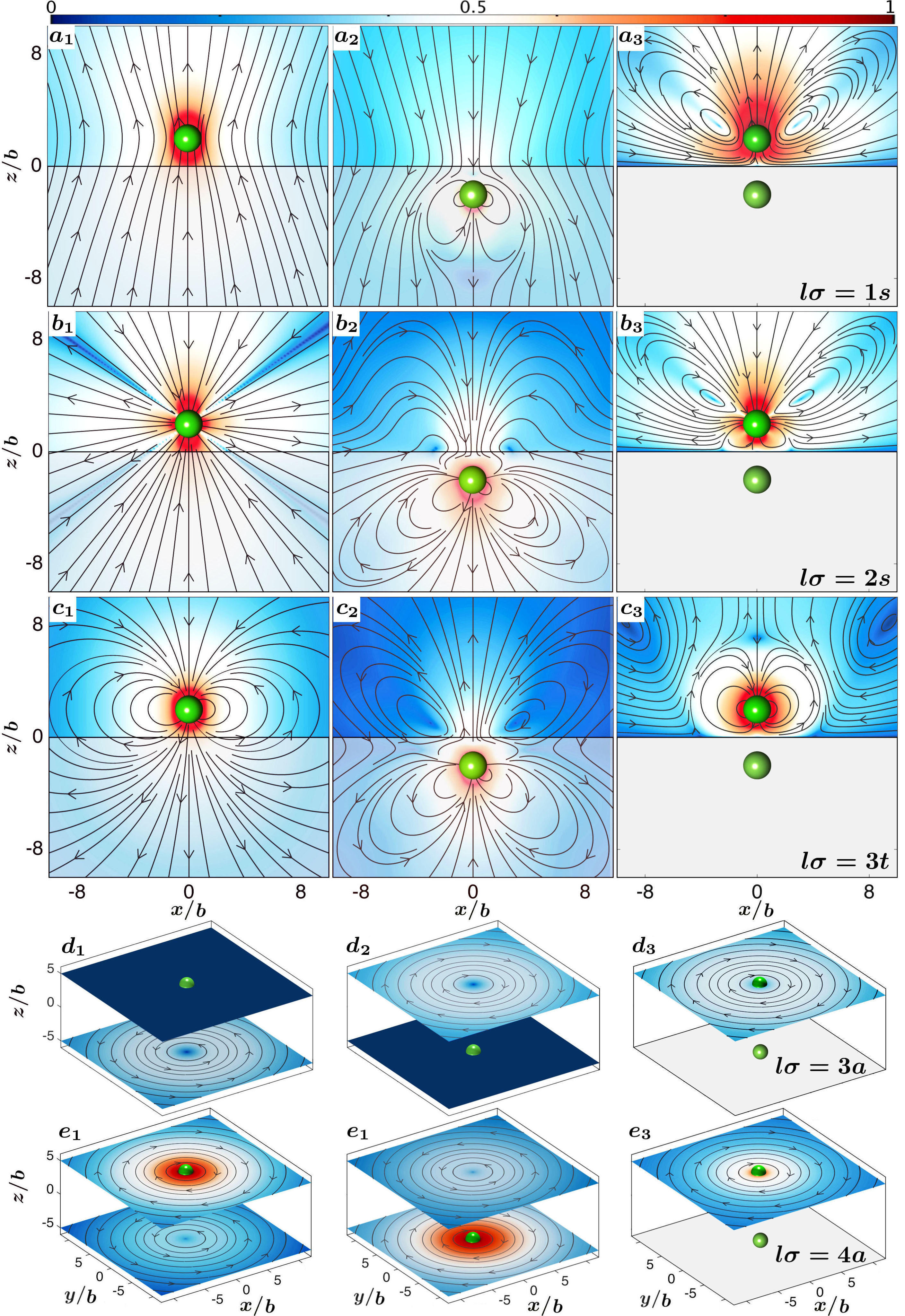
?figurename? 6: Irreducible axisymmetric and swirling components of fluid flow induced by an active colloid at a height $h$ from the wall. The streamlines of the fluid flow have been overlaid on the pseudo-color plot of the normalized logarithmic flow speed. The first column is the flow due to source alone while second column has the flow from the image, and their sum is plotted in the third column for all the irreducible modes, panel (a)-(e), used in this work. The first two rows show flow produced by a force monopole and a force dipole respectively. Third row is the flow due to a vector quadrupole, while the last two rows (panel d and e) are the swirling flows due to a torque dipole and antisymmetric octupole respectively. The torque-dipole and octupole induces a net rotation of colloids near a wall. The orientation of the colloid, in all these plots, is chosen to be along the wall normal. A linear combination of panel (a-c) has been used to plot the Fig. 1(a)-(c) .

References

Palacci et al. (2013)J. Palacci, S. Sacanna,
A. P. Steinberg, D. J. Pine, and P. M. Chaikin, Science 339, 936
(2013).
Singh and Adhikari (2016)R. Singh and R. Adhikari, arXiv:1603.05735 (2016).
(16) The active slip may have arbitrary
radial and tangential components, but the surface can not be a source or
sink .
(17) See supplemental material which contain explicit calculation supporting the results in the main text,
and at
https://goo.gl/QpBaHC
for movies of crystallization .
Ladyzhenskaia (1969)O. A. Ladyzhenskaia, The mathematical
theory of viscous incompressible flow, Mathematics and its applications (Gordon and Breach, 1969).
Pozrikidis (1992)C. Pozrikidis, Boundary Integral
and Singularity Methods for Linearized Viscous Flow (Cambridge University Press, 1992).
Kim and Karrila (1992)S. Kim and S. J. Karrila, Microhydrodynamics:
Principles and Selected Applications (Butterworth-Heinemann, 1992).
Langtangen and Wang (2012)H. P. Langtangen and L. Wang, Odespy, (2012).