Abstract

In these lectures we provide a basic introduction into the topic of dispersion relation and analyticity. The properties of 2-point functions are discussed in some detail from the viewpoint of the Källén-Lehmann and general dispersion relations. The Weinberg sum rules figure as an application. The analytic structure of higher point functions in perturbation theory are analysed through the Landau equations and the Cutkosky rules.

1 Prologue

Dispersion relations are a powerful non-perturbative tool which have originated in classical electrodynamics in the theory of Kramers-Kronig dispersion relations. Analytic properties follow from causality and the use of Cauchy’s theorem allows to obtain the real part of an amplitude from the knowledge of the imaginary part which is often better accessible. This is the idea of the S-matrix program from the fifties and sixties. Dispersion relations are sparsely discussed in modern textbooks as the focus is on other aspects of Quantum Field Theory (QFT). There are some excellent older textbooks on analyticity e.g. [1, 2, 3], some modern textbooks devote some chapters to the topic e.g.[4, 5], as well as some lecture notes [6]. I would hope that a student who has followed an introductory course on QFT or has read some chapters of a QFT textbook would be able to largely follow the presentation below.

1.1 Introduction

In the fifties and sixties QFT has found a big success in describing quantum electrodynamics (QED) thanks to the successful renormalisation program carried out by Dyson, Feynman, Schwinger, Tomonaga and others [7]. The description of the strong force with QFT proved to be difficult and there was some prejudice that a solution outside field theory had to be found. Two such approaches are dispersion theory using analytic properties [1] (Heisenberg, Chew, …) and Wilson’s operator product expansion [8]. As Weinberg remarks in his book [5] both of these approaches later became a part of QFT! By analytic properties we mean analyticity in the external momenta. In QFT analytic continuation is inherent in the field description (second quantisation). Let us remind ourselves how this is related to scattering matrix elements of particles.

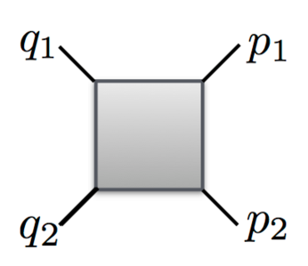
Figure 1: Schematic diagram for $2\to 2$ scattering corresponding to the matrix element in Eq. (1). Time goes from left to right.

A primary goal of particle physics is to describe scattering of $n$-particles via the so-called S-matrix. For the scattering of $2\to 2$ particles this reads (cf. Fig.1)

$$\phantom{a}_{\rm out}\langle p_{1},p_{2}|q_{1}q_{2}\rangle_{\rm in}=\phantom{a}_{\rm out}\langle p_{1},p_{2}|S|q_{1}q_{2}\rangle_{\rm out}\;,$$ (1)

where we have assumed the particles to be of spin $0$. In the case where they are all of equal mass this implies the following on-shell conditions: $p_{1}^{2}=p_{2}^{2}=q_{1}^{2}=q_{2}^{2}=m^{2}$. Hence one might wonder how analytic properties come into play. The answer is through the celebrated Lehman-Symmanzik-Zimmermann (LSZ) formula whose derivation can be found in most textbooks e.g. [4]. For our case it reads

$$\phantom{a}{}_{\rm out}\langle p_{1},p_{2}|q_{1}q_{2}\rangle_{\rm in} = -(iZ^{-1/2})^{4}\int_{x_{1},x_{2},y_{1},y_{2}}e^{-i(q_{1}\cdot x_{1}+q_{2}\cdot x_{2}-p_{1}\cdot y_{1}-p_{2}\cdot y_{2})}K_{x_{1}}K_{x_{2}}K_{y_{1}}K_{y_{2}}\times$$ (2)

$$\langle T\phi(x_{1})\phi(x_{2})\phi^{\dagger}(y_{1})\phi^{\dagger}(y_{1})\rangle+\text{disconnected terms}\;,$$

where $\int_{x}=\int d^{4}x$ hereafter, $T$ is the time ordering, $\langle\dots\rangle$ is the vacuum expectation value (VEV), the quanta are assumed to carry a charge (complex conjugation for outgoing particle), $K$ is the Klein-Gordon operator $K_{x_{1}}=\Box+m^{2}\to-(q_{1}^{2}-m^{2})$ and the $Z$ factor results from the asymptotic condition,

$$\langle 0|\phi(x)|q_{1}\rangle\stackrel{{\scriptstyle x_{0}\to\mp\infty}}{{\to}}Z^{1/2}\langle 0|\phi_{\text{in(out)}}(x)|q_{1}\rangle\;,$$ (3)

The asymptotic condition is the key idea of the LSZ-approach. Namely that when the particles are well separated from each other all that remains is the self-interaction which is parameterised by the renormalisation factor $Z$. The field $\phi$ is what is known as an interacting field whereas $\phi_{\text{in(out)}}$ are free fields in which case the right-hand side of the equation above equals $\sqrt{Z/(2\pi)^{3}}e^{-iq_{1}\cdot x}$. The disconnected part corresponds, for example, to the case where particle $q_{1}\to p_{1}$ and $q_{2}\to p_{2}$ without any interaction which is of no interest to us. From (2) we conclude that

• The scattering of $n$-particles ($n=n_{\rm in}+n_{\rm out}$) is described by $n$-point functions (or $n$-point correlators). The study of the latter is therefore of primary importance.

• The $n$-point correlators are functions of the external momenta e.g. $p_{1,2}^{2},q_{1,2}^{2},p_{1}\cdot p_{2},\dots$. First and foremost they are defined for real values or more precisely for real values with a small imaginary part e.g. $p_{1}^{2}={\rm Re}[p_{1}^{2}]+i0$. From there they can be analytically continued into the complex plane. Hence it is the second quantisation, describing particles with fields, that allows us to go off-shell for correlation functions.

The course consists of three parts. Analytic properties of 2-point functions (section 2), which comes with definite answer in terms of the non-perturbative Källén-Lehmann spectral representation. Applications of 2-point function in section 3. Last a short discussion of the analytic properties of higher point function in perturbation theory (PT) e.g. Landau equations and Cutkosky rules in section 4.

2 2-point Function

2.1 Dispersion Relation from $1^{\text{st}}$-principles: Källén-Lehmann Representation

Let us define the Fourier transform of the 2-point correlator as follows

$$\Gamma(p^{2})=i\int_{x}e^{ip\cdot x}\langle T\phi(x)\phi^{\dagger}(0)\rangle\;.$$ (4)

What determines the analytic structure of $\Gamma(p^{2})$? By analytic structure we mean the singularities e.g. poles, branch points and the associated branch cuts. The Källén-Lehmann representation [10, 11] gives a very definite answer to this question. The presentation is straightforward and can be found in most textbooks e.g. [5].

The 2-point function in the free and interacting case can be written as

$$\Gamma(p^{2})=\left\{\begin{array}[]{ll}\frac{1}{m^{2}-p^{2}-i0}=-\Delta_{F}(p^{2},m^{2})&\text{free}\\[8.5359pt] \frac{Z(\lambda)}{m^{2}-p^{2}-i0}+f(\lambda,p^{2})&\text{interacting}\end{array}\right.\;.$$ (5)

The function $Z(\lambda)$ and $f(\lambda,p^{2})$, where $\lambda$ is the coupling constant e.g. ${\cal L}_{\rm int}=\lambda\phi^{3}+{\rm h.c.}$, obey

$$Z(\lambda)\stackrel{{\scriptstyle\lambda\to 0}}{{\to}}1\;,\quad f(\lambda,p^{2})\stackrel{{\scriptstyle\lambda\to 0}}{{\to}}0\;,$$ (6)

in order to reproduce the free field theory limit. In what follows it is our goal to determine the properties of $f(\lambda,p^{2})$ in more detail. At the end of this section we are going to make remarks about the possible ranges of the $Z(\lambda)$-function. The first lesson to be learnt from the free field theory case is that it is the mass (i.e. the spectrum) which determines the analytic properties cf. Fig. 2(left). As we shall see this generalises to the interacting case.

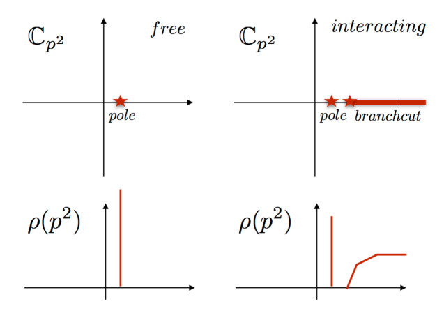
Figure 2: (left) analytic structure for free field theory propagator with spectral function underneath (right) idem for an interacting theory with a stable 1-particle state and a multiparticle-threshold

For technical reason it is advantageous to first study the positive frequency distribution

$$\langle\phi(x)\phi^{\dagger}(0)\rangle=\left\{\begin{array}[]{ll}\Delta_{+}(x^{2},m^{2})=\int\frac{d^{4}p}{(2\pi)^{3}}e^{-ip\cdot x}\delta^{+}(p^{2}-m^{2})&\text{free}\\[8.5359pt] (*)&\text{interacting}\end{array}\right.$$ (7)

where $\delta^{+}(p^{2}-m^{2})\equiv\delta(p^{2}-m^{2})\theta(p_{0})$ assures that energies are positive and that the momenta are on the mass-shell. It is the quantity $(*)$ that we intend to study. First we use the formal decomposition of the identity into a complete set of states $\mathbb{1}=\sum_{n}|n\rangle\langle n|$ which follow from unitarity. Inserting this relation and using translation invariance one gets

$$(*)=\sum_{n}e^{-ip_{n}\cdot x}|\underbrace{\langle 0|\phi(0)|n(p_{n})\rangle}_{\equiv f_{n}}|^{2}\;.$$ (8)

Further using $1=\frac{1}{(2\pi)^{4}}\int_{p}e^{-ip\cdot x}\int_{x}e^{ip\cdot x}$ and interchanging the $\sum_{n}$ and the $\int_{x}$ leads to

$$(*)=\int d^{4}pe^{-ip\cdot x}\underbrace{\equiv\sum_{n}\delta(p-p_{n})|f_{n}|^{2}}_{(2\pi)^{-3}\rho(p^{2})\theta(p_{0})}\;,$$ (9)

where $\rho(p^{2})$ is known as the spectral function, $(2\pi)^{-3}$ a convenient normalisation factor and $\theta(p_{0})$ assures positive energies which come from the positive energy condition on the external momentum. Upon using $\int_{p}F(p)=\int_{p}\int ds\delta(s-p^{2})F(s)$ and exchanging the $ds$ and $d^{4}p$ integration one finally gets

$$(*)=\int_{0}^{\infty}ds\rho(s)\Delta_{+}(x^{2},s)\;,$$ (10)

a spectral representation.

From (5) and (7) it seems plausible that this spectral representation generalises to the time ordered 2-point function as follows

At this stage we can make many relevant comments.

1. The Källén-Lehmann representation is a special case of dispersion relation. It shows that dispersion representation follow from first principles in QFT.

2. The analytic properties of $\Gamma(p^{2})$ are in one-to-one correspondence with the spectrum of the theory which is the answer to the question what determines the analytic properties of the 2-point function. Hence for the 2-point function there are no other singularities on the first sheet (known as the physical sheet) other than on the positive real axis determined by the spectrum. The analytic structure is depicted in Fig. 2(right). An example of an unphysical singularity (not on the physical sheet) is given in section 4.2.3.

3. The spectral function $\rho(s)\geq 0$ is positive definite as a direct consequence of unitarity. [As a homework question you could try to show that for a non-unitary theory with negative normed states (i.e. $\langle gh|gh\rangle=-1$ where “gh” stands for ghost) $\rho(s)$ loses positive definiteness.]

4. Often the spectral function is decomposed into a pole part

   $$\rho(s)=Z\delta(s-m^{2})+\theta(s-s_{0})\sigma(s)$$ (12)

   and continuum part $\sigma(s)$. The latter is the concrete realisation of the function $f(\lambda,s)$ in (5). In many applications $f_{0}$, the residue of the lowest state,

   $$\Gamma(p^{2})=\frac{|f_{0}|^{2}}{m^{2}-p^{2}-i0}+\int_{s_{0}}^{\infty}\frac{\sigma(s)}{m^{2}-p^{2}-i0}\;,$$ (13)

   is the non-perturbative quantity that is to be extracted. The left-hand side is computed and the $\sigma$-part is then either estimated or suppressed by applying an operation to the equation. This technique is the basis of QCD sum rules [12] and lattice QCD [13] extraction of low-lying hadronic parameters. In the former case the $\sigma$-part is suppressed by a Borel-transformation and in lattice QCD $\sigma$-part is exponentially suppressed in euclidian time.

5. The Källén-Lehmann representation straightforwardly applies to the case of a non-diagonal correlation function e.g. $\langle\phi_{A}(x)\phi_{B}^{\dagger}(0)\rangle$ but clearly positive definiteness is, in general, lost since $|f_{n}|^{2}\to f_{n}^{A}(f_{n}^{B})^{*}$.

6. As promised we return to the issue of interchanging various sums and integrals. This is of no consequence as long as there are no UV-divergences. As is well-known most field theories show UV-divergences so care has to be taken. UV-divergences demand regularisations and a prescription to renormalise the ambiguities which arise from removing the infinities. There are two ways to formally handle this problem. First, assuming a logarithmic divergence, we may amend (11) as

   $$\Gamma(p^{2})=\int_{0}^{\Lambda_{\rm UV}}ds\frac{\rho(s)}{s-p^{2}-i0}+A\;,$$ (14)

   where the so-called subtraction constant is adjusted to cancel the logarithmic divergence coming form the integral: $A=A_{0}\ln(\Lambda_{\rm UV}^{2}/\mu_{0}^{2})+A_{1}$ with $\mu_{0}$ being some arbitrary reference scale. The constant $A_{1}$ has either to be taken from experiment in the case where $\Gamma(p^{2})$ is physical (which implies scheme-independence) or is dependent on the scheme. The dependence in the latter case has to disappear when physical information is extracted from $\Gamma(p^{2})$. A more elegant way, in my opinion, is to handle the problem with a once subtracted dispersion

   $$\Gamma(p^{2})=\Gamma(p_{0}^{2})+(p^{2}-p_{0}^{2})\int_{0}^{\infty}ds\frac{\rho(s)}{(s-p^{2}-i0)(s-p_{0}^{2})}\;.$$ (15)

   It is observed that the integral is now convergent due to the extra $1/(s-p_{0}^{2})$ factor. The same remarks apply to $\Gamma(p_{0}^{2})$ as for the previously discussed $A_{1}$. To derive the above expression one writes an unsubtracted dispersion relation for $\Gamma(p^{2})$ and $\Gamma(p_{0}^{2})$ separately takes the difference and combines the fraction. They key point is that the divergent parts are the same and cancel each other.

7. Following the presentation in Weinberg’s book [5]: imposing the canonical commutation relation $[\partial_{t}\phi^{\dagger}(x),\phi(0)]_{x_{0}=0}=-i\delta(\vec{x})$ (in $\hbar=1$ units) leads to the sum rule

   $$\int_{0}^{\infty}ds\rho(s)=1\;,$$ (16)

   from where one deduces that:

   • $Z=1$ for a free theory

   • $0\leq Z\leq 1$ for an interacting theory

   • $Z=0$ if $\phi$ is a confined field

   The last case does not follow directly from (16) but is an important result due to Weinberg. An example is given by the quark propagator for which we do not expect a residue since it is a confined (coloured) particle. The fact that $Z_{\rm quark}\neq 0$ in each order in PT is a sign that the latter is not suited to describe the phenomenon of confinement.

8. By using causality, i.e. $\langle[\phi(x),\phi^{\dagger}(0)]\rangle=0$ for $x^{2}<0$ spacelike, it follows that $\bar{\rho}(s)=\rho(s)$ where $\bar{\rho}(s)$ is the antiparticle spectral function associated with $\Delta_{-}(x^{2},m^{2})=\langle\phi^{\dagger}(x)\phi(0)\rangle$. This is a special case of the CPT theorem. Related to this matter it was Gell-Mann, Goldberger and Thirring [14] in 1954 who derived analyticity properties from causality, for $\gamma+N\to\gamma+N$, justifying dispersion relations from a non-perturbative viewpoint.

2.2 Dispersion Relations and Cauchy’s Theorem

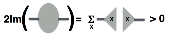
Figure 3: Standard sketch of optical theorem. The right-hand side is the sum over all intermediate states. It is a particular case of the cutting rules to be discussed in section 4.3.

It is our goal to characterise the spectral function $\rho(s)$ in other ways than through the spectrum. In preparation to the general case we are going to recite the optical theorem for the S-matrix. The S-matrix (1) is conveniently parameterised as

$$S=\mathbb{1}+iT\;,$$ (17)

where $T$ is the non trivial part of the scattering operator. From the unitarity of the S-matrix it follows that

$$\mathbb{1}=SS^{\dagger}=\mathbb{1}+\underbrace{i(T-T^{\dagger})}_{-2{\rm Im}[T]}+|T|^{2}\;,$$ (18)

if and only if

The right-hand side of the equation above is reminiscent of the spectral function in the case where $T$ is associated with $\phi$. Hence the expectation that $\rho(s)$ is related to an imaginary part is not unexpected from the viewpoint of the optical theorem. Below we are going to see that this is the case on very general grounds.

To do so we first take a little detour to discuss integral representations of arbitrary analytic functions by the use of Cauchy’s theorem. Let $f(p^{2})$ be an analytic function then by Cauchy’s theorem the following integral representation holds

$$f(p^{2})=\frac{1}{2\pi i}\int_{\gamma}\frac{ds\,f(s)}{s-p^{2}}\;,$$ (20)

provided that i) $p^{2}$ is inside the contour of $\gamma$ , ii) the contour of $\gamma$ does not cross any singularities.

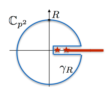
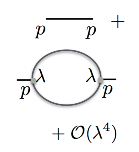
Figure 4: (left) Integration contour for 2-point function dispersion representation. (right) 2-point function in $\phi^{3}$ theory in perturbation theory.

Applying this techniques to the 2-point function in QFT one makes use of the knowledge of the analytic structure and chooses a contour $\gamma_{R}$ as in Fig. 4 which does not cross any singularities. The radius is then taken to infinity, $R\to\infty$, which in the case where there are UV divergences results in subtraction which we generically parameterised $P(p^{2})$ by a polynomial function (the $P=A$ in (14) is a constant polynomial). The integral is then written as

$$\Gamma(p^{2}) = \frac{1}{2\pi i}\int_{\gamma_{R}}\frac{ds\,\Gamma(s)}{s-p^{2}}\stackrel{{\scriptstyle R\to\infty}}{{\to}}\frac{1}{2\pi i}\int_{s_{1}}^{\infty}\frac{ds\,(\Gamma(s+i0)-\Gamma(s-i0))}{s-p^{2}}+P(p^{2})$$ (21)

$$= \frac{1}{2\pi i}\int_{s_{1}}^{\infty}\frac{ds\,{\rm disc}[\Gamma(s)]}{s-p^{2}-i0}+P(p^{2})=\frac{1}{\pi}\int_{s_{1}}^{\infty}\frac{ds\,{\rm Im}[\Gamma(s)]}{s-p^{2}-i0}+P(p^{2})\;,$$

where $s_{1}<\text{singularities}$ (to the left of red part in Fig. 4(left)) and the second line is the definition of what is called the discontinuity along the branch cut. The last equality follows from $2i{\rm Im}[\Gamma(s)]={\rm disc}[\Gamma(s)]$. This formula can be verified in each order in PT but is also justified on general grounds by the Schwartz reflection principle (cf. appendix A). In summary we then have that the spectral function is related to the the imaginary part and the discontinuity by

This equation follows from equating (11) and (21) and the knowledge that the subtraction constant are the same in both cases since they originate from UV divergences. Hence eliminating the contributions from the arc may result in UV-divergences and subtraction constants.

2.3 Dispersion Relations in Perturbation Theory

This section aims to illustrate (22) from the viewpoint of PT. In order to do PT one needs to specify a theory for which we choose ${\cal L}_{\rm int}=\lambda\phi^{3}+{\rm h.c.}$. The pole contribution is then just the propagator and the first non-trivial interaction is generated by the diagram in Fig. 4(right). The 1-loop graph is UV divergent and requires regularisation. Using dimensional regularisation $d=4-2\epsilon$ the result reads

$$\Gamma(p^{2})=\frac{Z(\lambda)}{m^{2}-p^{2}-i0}-\lambda^{2}|A|\left(\frac{1}{\epsilon}+2-\beta\ln\left(\frac{\beta+1}{\beta-1}\right)\right)+{\cal O}(\lambda^{4})\;,$$ (23)

with $\beta=\sqrt{1-(4m^{2}-i0)/p^{2}}$. The corresponding imaginary part divided by $\pi$ must be the spectral function

$$\rho(p^{2})\stackrel{{\scriptstyle\eqref{eq:main}}}{{=}}\frac{1}{\pi}{\rm Im}[\Gamma(p^{2})]\stackrel{{\scriptstyle\eqref{eq:above}}}{{=}}Z(\lambda)\delta(p^{2}-m^{2})+\lambda^{2}|A|\beta\theta(p^{2}-4m^{2})+{\cal O}(\lambda^{4})\;.$$ (24)

The UV divergence is not important for our purposes since it does not affect the imaginary part. Of course the UV-divergence means that the dispersion relation does not converge in the UV. This problem can be handled either by a subtracted dispersion relation or a polynomial counterterm and regularisation as discussed under point 6 in section 2.1.

Having resolved this technical issue we focus on the interpretation of the imaginary part. The propagator term is a pole singularity with a delta function in the spectral function and the logarithm corresponds to a branch cut singularity resulting in a $\theta$-function part. By the spectral representation (3.1) this branch cut must correspond to some physical intermediate state. This state is a 2-particle state starting at the minimum centre of mass energy $4m^{2}$ ranging all the way up to infinity. The precise value depends on the corresponding momentum configuration. Let the two particle momenta be parameterised by

$$p_{1,2}=(\sqrt{m^{2}+x^{2}},0,0,\pm x)\;,\quad x>0\;,\quad p_{1,2}^{2}=m^{2}\;,\quad p^{2}=(p_{1}+p_{2})^{2}=4m^{2}+4x^{2}$$ (25)

and therefore $4x^{2}=p^{2}-4m^{2}$ which can be satisfied for any (arbitrarily large) $p^{2}\geq 4m^{2}$.

3 Application of $2$-point Functions

There are numerous applications of $2$-point functions and dispersion relations. For example deep-inelastic scattering, QCD sum rules which we have alluded to in and below (13), $e^{+}e^{-}\to\text{hadrons}$ and inclusive $b\to X_{u,c}\ell\nu$ decays with the additional assumption of analytic continuation to Minkowski-space. We choose to present the Weinberg sum rules (WSR).

3.1 Weinberg Sum Rules

The Weinberg sum rules are an ingenious construction involving a variety of conceptual ideas. They were proposed in 1967 by Weinberg [15] in the pre-QCD era but we are going to present them from the viewpoint of QCD e.g. [6, 16]. One considers the correlation function of left and right-handed current with two massless quark flavours

$$i\int d^{4}xe^{iq\cdot x}\langle TJ^{a,L}_{\mu}(x)J^{b,R}_{\nu}(x)\rangle=(q_{\mu}q_{\nu}-q^{2}g_{\mu\nu})\Pi^{a,b}_{\rm LR}(q^{2})\;,$$ (26)

where

$$J^{a,(L,R)}_{\mu}=\bar{q}T^{a}\gamma_{\mu}q_{L,R}\;,$$ (27)

with $q_{L,R}=P_{L,R}q$, $P_{L,R}=1/2(1\mp\gamma_{5})$, $T^{a}$ being an $SU(2)$-generator (Pauli-matrix). The Lorentz-decomposition in (26) is valid in the limit of massless quarks. According to the previous sections the function $\Pi^{a,b}_{\rm LR}(-Q^{2})$, with $-q^{2}=Q^{2}>0$ satisfies a dispersion relation of the form

$$\Pi^{a,b}_{\rm LR}(-Q^{2})=\frac{1}{\pi}\int_{s_{0}}^{\infty}\frac{ds\,{\rm Im}[\Pi^{a,b}_{\rm LR}(s)]}{s+Q^{2}}+A$$ (28)

where $A$ is a subtraction constant due to the potential logarithmic divergence which may arise since $\Pi^{a,b}_{\rm LR}$ is of mass dimension zero.

The peculiarity of the WSR relies on the absence of lower dimension corrections in the OPE. This can be seen in an elegant manner using $SU(2)$ representation theory. We denote by $1,F$ and $A$ the trivial, fundamental and adjoint representation of $SU(2)$ which are of dimension $1,2$ and $3$. The correlation function is in the (A,A)-representation of the $(SU(2)_{L},SU(2)_{R})$ global flavour symmetry. The individual OPE-contribution must be in the same global flavour symmetry representation or vanish otherwise.

One considers Wilson’s OPE in momentum space, valid for $Q^{2}=-q^{2}\gg\Lambda_{\rm QCD}^{2}$

$$\Pi^{a,b}_{\rm LR}(-Q^{2})=C_{\mathbb{1}}(Q^{2})\langle\mathbb{1}\rangle+C_{\bar{q}q}(Q^{2})\frac{(\langle\bar{q}^{a}_{L}q^{b}_{R}\rangle+{\rm h.c.})}{Q^{3}}+C_{JJ}(Q^{2})\frac{\langle J^{L,a}_{\mu}J^{R,b}_{\mu}\rangle}{Q^{6}}+{\cal O}\left(\frac{\Lambda_{\rm QCD}^{8}}{Q^{8}}\right)\;.$$ (29)

The functions $C(Q^{2})$ are known as Wilson coefficients and carry logarithmic correction in QCD. As can be seen from the formula above the condensate terms of dimension $d$ are suppressed by $1/Q^{d}$ relative to the identity term. The $\langle\mathbb{1}\rangle$-term corresponds to PT and the condensates, i.e. VEVs of operators, are of non-perturbative nature. The former is in $(1,1)$-representation and therefore absent. A quark bilinear $\langle\bar{q}^{a}_{L}q^{b}_{R}\rangle$ is in the $(F,F)$-representation and absent for the same reason. The dimension six operator is, somewhat trivially, in the $(A,A)$-representation and therefore the leading term appears at ${\cal O}(1/Q^{6})$. The vanishing of the $1/Q^{2}$- and $1/Q^{4}$-terms lead to constraints. The latter can be obtained by expanding the denominator in inverse powers of $Q^{2}$,

$$\frac{1}{s+Q^{2}}=\frac{1}{Q^{2}}\frac{1}{1+s/Q^{2}}=\frac{1}{Q^{2}}-\frac{s}{Q^{4}}+\frac{s^{2}}{Q^{6}}+\dots\;.$$ (30)

Note the absence of the perturbative term means in particular that there is no UV-divergence and hence $A=0$. Since the convergence is two powers in $s$ higher (1st and 2nd WSR) the dispersion relation is referred to a as superconvergent.

The WSR (31) are a powerful non-perturbative constraint. We present the original application pursued by Weinberg. First we notice that the left-right correlator can be written as a difference of the vector and axial correlator

$$\Pi^{a,b}_{\rm LR}(s)=\frac{1}{4}\left(\Pi^{a,b}_{\rm VV}(s)-\Pi^{a,b}_{\rm AA}(s)\right)\;,$$ (32)

where $J^{V(A),a}_{\mu}\equiv\bar{q}T^{a}\gamma_{\mu}(\gamma_{5})q$. Taking into account the lowest lying particles $\pi$, $\rho$ and $a_{1}$ in the narrow width approximation and assuming isospin symmetry (i.e. global $SU(2)_{V}$ -flavour symmetry) one arrives at

$$\rho_{V}^{a,b}(s) \;=\; \frac{1}{\pi}{\rm Im}[\Pi^{a,b}_{\rm VV}](s)=\delta^{ab}(f_{\rho}^{2}\delta(s-m_{\rho}^{2})+\theta(s-s_{0})\sigma_{V})\;,$$

$$\rho_{A}^{a,b}(s) \;=\; \frac{1}{\pi}{\rm Im}[\Pi^{a,b}_{\rm AA}](s)=\delta^{ab}(f_{\pi}^{2}\delta(s)+f_{a_{1}}^{2}\delta(s-m_{a_{1}}^{2})+\theta(s-s_{0})\sigma_{A})\;.$$ (33)

The functions $\sigma_{V,A}$ contain any higher states and multiparticle states. If one assumes that around $s_{0}$ perturbation theory is valid then $\rho_{\rm LR}(s)=0$ for $s>s_{0}$ which in turn implies $\sigma_{V}=\sigma_{A}$.

Hence using (3.1) the two WSR (31) read

$$f_{\rho}^{2}=f_{\pi}^{2}+f_{a_{1}}^{2}\;,\qquad m_{\rho}^{2}f_{\rho}^{2}=m_{a_{1}}^{2}f_{a_{1}}^{2}\;,$$ (34)

where the decay constants are defined as

$$\langle\rho[a_{1}]^{b}(p)|J^{V[A],a}_{\mu}|0\rangle=\delta^{ab}\eta_{\mu}(p)m_{\rho[a_{1}]}f_{\rho[a_{1}]}\;,\quad\langle\pi^{b}(p)|J^{A,a}_{\mu}|0\rangle=\delta^{ab}p_{\mu}f_{\pi}\;,$$ (35)

with $\eta$ being the polarisation vector.

In his original paper Weinberg used the experimentally motivated KSFR relation $f_{\rho}^{2}=2f_{\pi}^{2}$ which then leads to $m_{a_{1}}=\sqrt{2}m_{\rho}$. This relation is reasonably satisfied by experiment: $m_{a_{1}}/m_{\rho}\simeq 1.63\simeq 1.15\sqrt{2}$. Let us end this section with mentioning two further applications of this reasoning.

• Being related to chirality the WSR, or the $\Pi_{LR}$ function, is a measure of contributions to electroweak precision measurement in the case of physics beyond the Standard Model coupling to new fermions. The WSR serve to estimate the contribution of strongly coupled extensions of the standard model such as technicolor and the composite Higgs model.

• The inverse moments of the spectral function, with pion pole subtracted, are related to the low energy constant $L_{10}$ of chiral perturbation theory. Note, chiral perturbation theory is an expansion in $Q^{2}$, and not $1/Q^{2}$ as the OPE, and thus leads to inverse moments rather than moments themselves. It is not the WSR per se which are important in this respect but the onset of the duality threshold of PT-QCD which allows to estimate $L_{10}$ in terms of $f_{\pi,\rho,a_{1}}$. The estimate of $L_{10}$ obtained is in reasonable agreement with experiment.

At this point the students were given the choice of continuing with applications (e.g. infrared interpretation of the chiral anomaly, positivity of low energy constants …) or a the more conceptual topic of higher point functions properties. Their choice was the latter.

4 Analyticity Properties of higher point Functions

There are many motivations to study higher point functions and their analytic structure amongst which we quote the following:

• As seen in the introduction they describe the scattering of $n$-particles.

• From the discussion in section 2.2 it is clear that to write down dispersion relations one needs to know first and foremost the analytic structure of the amplitude in question.

• 3-point functions are relevant for the study of form factors. Consider for example the $B\to\pi$ form factor, relevant for the determination of the CKM-element $|V_{\rm ub}|$, defined by

  $$\langle\pi(p)|V_{\mu}|B(p_{B})\rangle=(p_{B})_{\mu}f^{B\to\pi}_{+}(q^{2})+\dots\;,$$ (36)

  where the dots stand for the other Lorentz structure and $V_{\mu}=\bar{b}\gamma_{\mu}u$ is the weak current (the axial part does not contribute in QCD by parity conservation). Then the form factor can be extracted from the following 3-point function, by using a double dispersion relation (dispersion relation in the $p_{B}^{2}$ and $p^{2}$-variable)

  $$\Gamma(p^{2},p_{B}^{2},q^{2}) \;=\; i^{2}\int_{x,y}e^{-i(p_{B}\cdot x-p\cdot y)}\langle TJ_{B}(x)J_{\pi}(y)V_{\mu}(0)\rangle\;,$$ (37)

  $$\;=\; (p_{B})_{\mu}\left(\frac{g_{\pi}\,f_{B}\,f_{+}^{B\to\pi}(q^{2})}{(p_{B}^{2}-m_{B}^{2})(p^{2}-m_{\pi}^{2})}+\text{higher}\right)+\dots\;,$$

  where “higher” stands for higher contributions in the spectrum (the analogue of $\sigma(s)$ in (24)) and

  $$J_{B} \;=\; \bar{q}i\gamma_{5}b\;,\quad \langle B|J_{B}|0\rangle \;=\; f_{B}\;,$$

  $$J_{\pi} \;=\; \bar{q}i\gamma_{5}q\;,\quad \langle 0|J_{\pi}|\pi\rangle \;=\; g_{\pi}\;,$$ (38)

  play the role of the interpolating operators of the LSZ-formalism cf. footnote 2. As previously mentioned the key idea is then to compute $\Gamma(p^{2},p_{B}^{2},q^{2})$ in some formalism and to find ways to either estimate or suppress the higher states in order to extract the form factor where $g_{\pi}$ and $f_{B}$ are assumed to be known quantities.

  In fact if we were able to compute $\Gamma(p^{2},p_{B}^{2},q^{2})$ with arbitrary precision then the function would assume the form in (37) and we could simply extract the form factor from the limiting expression

  $$f_{+}^{B\to\pi}(q^{2})=\frac{1}{g_{\pi}f_{B}}\lim_{p_{B}^{2}\to m_{B}^{2},p^{2}\to m_{\pi}^{2}}(p_{B}^{2}-m_{B}^{2})(p^{2}-m_{\pi}^{2})\Gamma(p^{2},p_{B}^{2},q^{2})\;,$$ (39)

  which makes the connection to the LSZ-formalism (2) apparent. Unfortunately at present we cannot hope to do so and therefore we have to resort to the approximate techniques as alluded to above.

We have seen that for the 2-point function the analytic structure of the first sheet (physical sheet) is fully understood through the Källén-Lehmann representation. Moreover the singularities on the physical sheet are in one-to-one correspondence with the physical spectrum. For higher point function less is known in all generality. We refer the reader to the works of Källén-Wightman [17] and Källén [18] for some general studies of 3- and 4-point functions using first principles and the summary by Andrè Martin [19] for a comparatively recent survey of rigorous results.

Hence one has to become immediately more modest! We are going to restrain ourselves to analysing singularities in PT for physical momenta (i.e. real momenta). This is done by the use of two major tools:

• Landau equations: which answer the question about the location of the singularities cf. section 4.2. The question on which sheet the singularities are is a difficult question which we comment on.

• Cutkosky rules: are rules for computing the discontinuity of an amplitude cf. section 4.3.

Before analysing these matters in more details let us first consider the normal-thresholds for higher point functions.

4.1 Normal Thresholds: cutting Diagrams into two Pieces

The so-called normal thresholds are directly associated with unitarity. They originate from cutting (to be made more precise when discussing the Cutkosky rules) the diagram into two pieces and generalise the equal size optical theorems cuts. Cutting a diagram into two pieces is equivalent to the combinatorial problem of grouping the external momenta into two sets. Tab. 1 provides the overview of the number of cuts versus number of independent kinematic variables. For the two lowest functions there are no constraints whereas for all higher point functions there are constraints due to momentum conservation. For the $4$-point functions this constraint is known as the famous Mandelstam constraint

$$\sum_{i=1}^{4}p_{i}^{2}=s+t+u\;,\quad s=(p_{1}+p_{2})^{2}\;,\quad t=(p_{1}+p_{3})^{2}\;,\quad u=(p_{1}+p_{4})^{2}\;,$$ (40)

where we choose conventions such that all momenta are incoming (momentum conservation reads $\sum_{i=1}^{4}(p_{i})_{\mu}=0$).

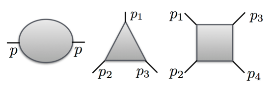
Figure 5: Sketch of generic $2,3,4$-point function. The number of unitarity cuts and independent kinematic variables are listed in Tab. 1.

The fact that the amplitudes become functions of several complex variables makes matters more difficult. For example:

• From the Mandelstam constraint it can be seen that the unitarity cuts from one channel do appear on the negative real axis in the complex plane of another channel. Say the $u$-channel cuts, with forward kinematics $t=0$, do appear on the negative real axis in the complex plane of $s=\sum_{i}m_{i}^{2}-u$ ($p_{i}^{2}=m_{i}^{2}$ on shell). These $u$-channel cuts in the $s$-plane are sometimes referred to as left-hand cuts as opposed to the proper $s$-channel unitarity cuts on the right-hand side of the complex plane (cf. Fig. 4).

• Several complex variables allow for dispersion relations in multiple channels. An example of which is the conjectured Mandelstam representation, cf. [4, 1], which is a double dispersion relation.

• There are cuts which are not directly related to unitarity, so-called anomalous thresholds, cutting the diagram into more than 2 pieces. We will return to the latter briefly when discussing the Landau equations and Cutkosky rules.

$$\begin{array}[]{c | c | c | c }n\text{-point function}&\text{\#cuts}&\text{\#variables}&\text{\#constraints}\\ \hline\cr 2&1&1&0\\ 3&3&3&0\\ 4&7&6&1\\ 5&15&10&5\end{array}$$

Table 1: The number (=#) of unitarity cuts equals the number of independent variables plus the number of constraints. Cf. Fig. 5 some diagrams. For the $2$- and $3$-point functions there are no constraints whereas for the $4$-point function there is the famous Mandelstam constraint (40). Generally for $n\geq 4$ the number of invariants is $4n-10$ where $4n$ corresponds to all the components of the four momenta and $10$ subtracts the Lorentz-symmetries. (For $n\leq 4$ the formula reads $n(n-1)/2$ which gives a larger number since not all the Lorentz symmetries can be used for reduction of parameters). For the $5$-point function the reduction from 15 cuts to 10 independent variables follows from multiple use of the Mandelstam relation (40) on subtopologies of the kinematic diagram e.g.[20].

4.2 Landau Equations

Before stating the Landau equations it is useful to look at singularities of a one-variable integral representation where the integrand has pole singularities as a function of external parameters. The Landau equations originate from analysing this problem for the integrals of several variables appearing in PT. The presentation in this section closely follows the original paper [21] and the textbook[1].

4.2.1 Singularities of one-variable Integral Representations

Consider the following integral representation of a analytic function $f(z)$

$$f(z)=\int_{\gamma_{ab}}g(z,w)dw\;,$$ (41)

where the integrand $g(z,w)$ contains pole singularities $w_{i}(z)$ which depend on $z$. The path $\gamma_{ab}$ ranges from a point $a$ to $b$ and does not cross any singularities for some $z=z_{0}$ as shown in Fig. 6(left). The analytic properties of $f(z)$ depend on whether or not the path $\gamma_{ab}$ can be smoothly deformed away from approaching pole singularities $\omega(z_{i})$.

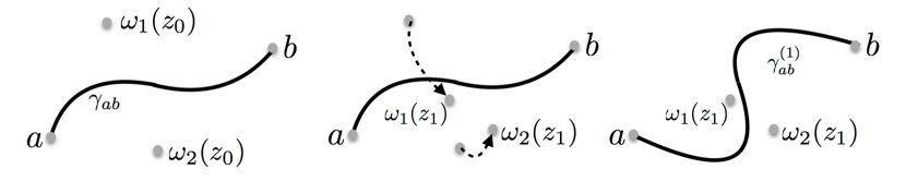
Figure 6: Path $\gamma_{ab}$ between endpoints $a$ and $b$. (left) Poles $\omega_{1,2}(z_{0})$ of the integrand $g(z,\omega)$ in (41) for $z=z_{0}$ (middle) Deformation of poles $\omega_{1,2}$ by the parameter $z_{0}$ to $z_{1}$. This is not provide an analytic continuation of the function $f(z)$ around $z_{0}$ to $z_{1}$. (right) deformation of path $\gamma_{ab}$ to $\gamma_{ab}^{(1)}$ serves as a (legitimate) analytic continuation of the function $f(z)$ in (41) around $z_{0}$ to $z_{1}$.

For example, if we start from $z=z_{0}$ and go to $z=z_{1}$ with $\omega(z_{1})$ crossing the $\gamma_{ab}$ (cf. Fig. 6(middle)) then the path $\gamma_{ab}$ can be smoothly deformed as in Fig. 6(right) and this constitutes an analytic continuation of the function $f(z)$. There are though instances when this is not possible:

• When a singularity $w_{i}(z)$ approaches one of the endpoints $a$ or $b$; e.g. $w_{i}(z_{1})=a$ Fig. 7(left). This case is known as an endpoint singularity.

• When two singularities approach each other, $w_{1}(z_{1})=w_{2}(z_{1})$ from different direction of the integration path as depicted in Fig. 7(right). This case is known as a pinch singularity.

• When the path needs to be deformed to infinity (can be reduced to case b).

In PT it is the pinch singularity type that gives rise to the singularities.

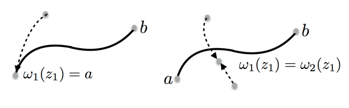
Figure 7: (left) endpoint singularity (right) pinch singularity

4.2.2 Landau Equations = several-variable Case

Landau [21] and others (cf. [1] for further references ) have analysed the problem of singularities, discussed for a single integral above, for the case of several variables in the context of Feynman graphs. A generic Feynman graph of $L$-loop of momenta $k_{i}$ ($i=1\dots L$), $N$-propagators, external momenta $p_{i}$ (cf. Fig. 8(left) for a representative graph) can be written as follows

$$I=\int Dk\frac{1}{\prod_{i=1}^{N}(q_{i}^{2}-m_{i}^{2}+i0)}\;,\qquad Dk=\prod_{i=1}^{L}d^{4}k_{i}\;,$$ (42)

where $q_{i}=q_{i}(p_{j},k_{l})$ are the momenta of the propagators. By the technique of Feynman parameters (generalisation of $(AB)^{-1}=\int_{0}^{1}d\alpha(\alpha A+(1-\alpha)B)^{-2}$) one may rewrite $I$ as follows

$$I=\int Dk\int_{0}^{1}D\alpha\frac{1}{(F+i0)^{N}}\;,\qquad D\alpha=\prod_{i=1}^{N}d\alpha_{i}\delta(1-\sum_{i=1}^{N}\alpha_{i})\;,$$ (43)

where the crucial denominator $F$ reads

$$F=\sum_{i=1}^{N}\alpha_{i}(q_{i}^{2}-m_{i}^{2})\;.$$ (44)

Is seems worthwhile to emphasise that even though these formulae look rather involved they are completely straightforward.

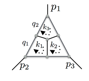
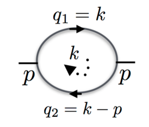
Figure 8: (left) Generic Feynman diagram aimed to clarify notation used in text (right) bubble graph discussed in the text

The key idea is that there are different types of singularities depending on how many of the $N$ propagators are on shell, i.e. $q_{i}^{2}-m_{i}^{2}$. It is the number of on-shell propagators which serves as a classification of the singularities. The Landau equations in condensed form are:

We are not going to show a proof of the Landau equations but state the result and argue for its plausibility below. Let us emphasise that the Landau equations neither tell us on which sheet the singularities are (cf. section 4.2.3 for the refinement in this direction) nor how to compute the discontinuity relevant for the dispersion relations (cf. Cutkosky rules section 4.3). The first condition assures that $F=0$ by demanding that each summand is zero in (44). The interpretation of $q_{i}^{2}=m_{i}^{2}$ is of course that the corresponding propagator is on-shell and contributes to the singularity. Correspondingly $\alpha_{i}=0$ means that the corresponding line does not enter the singularity. In Fig. 11 we give an example of a 3-point function cut. The second condition (46) has a geometric interpretation. It means that the corresponding singularity surfaces are parallel to each other and that the hypercontour can therefore not be deformed away from the approaching singularity surfaces. This is the analogy of the pinch singularity discussed in section 4.2.1. Eq. (46) can be cast into a more convenient form by contracting the equation by a vector $(q_{j})_{\mu}$ which leads to the matrix equatons

$$\text{[ii']}\quad Q\vec{\alpha}=0\;,\qquad(Q)_{ij}=q_{i}\cdot q_{j}\;,\quad(\vec{\alpha})_{i}=\alpha_{i}\;.$$ (47)

For non-trivial $\vec{\alpha}$ the second Landau equation is then solved by demanding that the so-called Cayley-determinant $\rm detQ=0$ vanishes.

4.2.3 Landau Equation exemplified: 1-loop 2-point Function (bubble graph)

Consider the bubble graph depicted in Fig. 8(right) with external momenta $p$, loop momenta $k$ and momenta $q_{1}=k$ and $q_{2}=k-p$. The first Landau equation (45) tells us that [As a homework you could ask yourself why the case $\alpha_{1}=0$ and $q_{2}^{2}=m_{2}^{2}$ is not an option for a singularity] $q_{1}^{2}=m_{1}^{2}$ and $q_{2}^{2}=m_{2}^{2}$. The second Landau equation (47) can be cast into the form $\det Q=0$

$$\det Q=\det\left(\begin{matrix}m_{1}^{2}&q_{1}\cdot q_{2}\\ q_{1}\cdot q_{2}&m_{2}^{2}\end{matrix}\right)=0\quad\Leftrightarrow q_{1}\cdot q_{2}=\pm m_{1}m_{2}$$ (48)

which we may reinsert back into $p=q_{1}+q_{2}$ which yields the two singularities $p_{(+)}^{2}=(m_{1}+m_{2})^{2}$ and $p_{(-)}^{2}=(m_{1}-m_{2})^{2}$,

$$p^{2}=(q_{1}-q_{2})^{2}=q_{1}^{2}-2q_{1}\cdot q_{2}+q_{2}^{2}=(m_{1}\mp m_{2})^{2}\;.$$ (49)

This might surprise us at first since from unitarity we expect there to be a branch point at $p_{(+)}^{2}$ but the point $p_{(-)}^{2}<p_{(+)}^{2}$ has no place in this picture. The resolution comes upon recalling that the Landau equations inform us about the singularities but do not tell us on which sheet they are! In order to learn more we may solve $Q\vec{\alpha}=0$ with $\vec{\alpha}=(\alpha,(1-\alpha))^{T}$ which gives

$$\alpha_{\pm}=\frac{m_{2}}{m_{2}\pm m_{1}}\Rightarrow\quad 0<\alpha_{+}<1\;,\quad\alpha_{-}>1\text{ or }\alpha_{-}<0\;,$$ (50)

for $m_{1,2}>0$. From this we learn that $\alpha_{+}$ is within the integration region (recall $\int_{0}^{1}D\alpha$ (43)) and $p_{(+)}^{2}$ is therefore on the physical sheet, wheras $\alpha_{-}$ is outside the integration region necessitating the deformation of the $\alpha$-contour. This indicates that $\alpha_{-}$ may not be on the physical sheet as the contour may crosses singularities in the course of deformation. The singularity $p_{(-)}^{2}=(m_{1}-m_{2})^{2}$ is sometimes referred to as a pseudo threshold. These findings suggest an important refinement of the Landau conditions.

For non physical configuration, complex momenta, the situation is far from straightforward to say the least. The method of choice is often deformation to a case of a physical configuration and then deform to complex momenta checking whether or not singularities are crossed in that process. Crossing a singularity correspond to changing the Riemann sheet. Alternatively one can deform the masses to complex values keeping the $\alpha_{i}\in[0,1]$ and then deform back.

Geometric interpretation and the forgotten second type singularity

We take a detour and give a geometrical interpretation of the singularities of the bubble graph. The first and second Landau equations (45,46) read

$$(k-p)^{2}=m_{1}^{2}\;,\quad k^{2}=m_{2}^{2}\;,\quad\alpha k_{\mu}+(1-\alpha)(k-p)_{\mu}=0\;.$$ (51)

The first Landau equation defines two hyperboloids with centres displaced by $p$ with respect to each other. The second Landau equation assures that $p$ and $k$ are parallel. First we discuss the previously found solutions and then uncover the forgotten second type singularity.

• Normal and pseudo threshold
  Equations (51) are satisfied when the two hyperboloids touch each other at the symmetric point with displacement in the $k_{0}$-direction. The displacement is given by $p_{(\pm)}^{2}=(m_{1}\pm m_{2},0,0,0)^{2}=(m_{1}\pm m_{2})^{2}$ in the case where the hyperboloids open up in opposite and the same direction respectively. We refer the reader to Fig. 9 (left) and (middle) for an illustration and the relevant equations in the caption.

• Second type singularity
  Fig. 9 (right) shows yet another type of singularity. For any light-like displacement $p$, the two hyperboloids meet at infinity. These type of singularities were first noted by Cutkosky [22] who named them non-Landauian singularities whereas nowadays they are known as second type singularities [1]. The Cayley-determinant is zero since $q_{1}$ and $q_{2}$ are parallel with $k$ and $p$ being light-like. If we parameterise $p/k=\epsilon$ then the second Landau equation is satisfied when $\alpha=(1+\epsilon)/\epsilon$ which diverges when $\epsilon\to 0$ and in particular outside the $[0,1]$-interval. Hence the singularity may therefore not be on the physical sheet. More directly the singularity $p_{(0)}^{2}=0$ has no interpretation in terms of the spectrum. By the one-to-one relation of the spectrum and the 2-point function singularities (cf. Källén-Lehmann representation in section 2) it is to be concluded that this singularity is not on the physical sheet.

More generally second type singularities are determined by the vanishing of the Gram-determinant $\det p_{i}\cdot p_{j}=0$ (where the $p_{i}$ are the external momenta) [1]. The singularity $p_{(0)}^{2}=0$ for the bubble-graph is then just the solution of the one-dimensional Gram-determinant. In summary second-type singularities are therefore independent of the masses and not on the physical sheet.

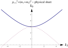
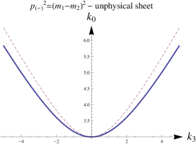
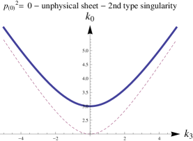
Figure 9: Choosen $m_{1}=3$ and $m_{2}=2$ in arbitrary units. (left) Normal threshold: $k_{0}=\sqrt{k_{3}^{2}+m_{1}^{2}}$ and $k_{0}=(m_{1}+m_{2})-\sqrt{k_{3}^{2}+m_{2}^{2}}$ and $p_{+}=(m_{1}+m_{2},0,0,0)$. (middle) Pseudo threshold: $k_{0}=\sqrt{k_{3}^{2}+m_{1}^{2}}$ and $k_{0}=(m_{1}-m_{2})+\sqrt{k_{3}^{2}+m_{2}^{2}}$ and $p_{-}=(m_{1}-m_{2},0,0,0)$. (right) Second type singularity: $k_{0}=\sqrt{k_{3}^{2}+m_{1}^{2}}$ and $k_{0}=\sqrt{k_{3}^{2}+m_{2}^{2}}$ and $p_{(0)}=(0,0,0,0)$ the two curves meet at infinity and are independent of the masses. It is obvious that any light-like $p$, e.g. $p_{(0)}=(x,0,0,x)$ for $x$ real, is also a valid parametrisation.

Discussion upon using explicit 1-loop result:

After these abstract considerations we consider it advantageous to illustrate these type of singularities explicitly. The bubble graph

$$B_{0}(p^{2},m_{1}^{2},m_{2}^{2})=\frac{4\pi^{2}}{i}\int\frac{d^{4}k}{(2\pi)^{4}}\frac{1}{(k-p)^{2}-m_{1}^{2}+i0)(k^{2}-m_{2}^{2}+i0)}\;,$$ (52)

is UV-divergent. In order to avoid regularisation we may use the same trick as for the subtracted dispersion relation and take the difference with a fixed value. The results, valid on the physical sheet, reads (e.g. [4])

$$B_{0}(p^{2},m_{1}^{2},m_{2}^{2})-B_{0}(\bar{p}^{2},m_{1}^{2},m_{2}^{2})=\frac{1}{2p^{2}}\left[X(p^{2},m_{1},m_{2})-X(0,m_{1},m_{2})\right]-[p^{2}\leftrightarrow\bar{p}^{2}]\;,$$ (53)

where $\bar{p}^{2}$ is the arbitrary subtraction point,

$$X(p^{2},m_{1},m_{2})=\sqrt{\lambda}\ln\left(\frac{\sqrt{(m_{1}+m_{2})^{2}-p^{2}}+\sqrt{(m_{1}-m_{2})^{2}-p^{2}}}{\sqrt{(m_{1}+m_{2})^{2}-p^{2}}-\sqrt{(m_{1}-m_{2})^{2}-p^{2}}}\right)^{2}$$ (54)

and $\lambda=(p^{2}-(m_{1}+m_{2})^{2})(p^{2}-(m_{1}-m_{2})^{2})$ the Källén-function and not to be confused with a coupling constant. It is noted that the expression above is consistent with (23) in the limit $m=m_{1}=m_{2}$. We can learn three things from the representation (53). On the physical sheet: (i) there is a branch cut starting at $p^{2}\geq(m_{1}+m_{2})^{2}$ (normal threshold) (ii) there is no branch cut at $p^{2}=(m_{1}-m_{2})^{2}$ (pseudo threshold) and (iii) there is no singularity for $p^{2}\to 0$ (second type singularity). To see the correctness of (ii) one has to note that $\sqrt{\lambda}$ is imaginary for $(m_{1}-m_{2})^{2}<p^{2}<(m_{1}+m_{2})^{2}$. In summary it is confirmed from the explicit representation (53) that the pseudo threshold and the second type singularity are, indeed, not present on the physical sheet.

4.3 Cutkosky rules

The question of how to compute the actual singularities for physical configurations is answered by the cutting rules stated by Cutkosky [22] shortly after the Landau equations were formulated. This is by no means accidental as they are closely related. The Landau equations tell us that there is a singularity if either $q_{i}^{2}=m_{i}^{2}$ or $\alpha_{i}=0$ (45) and the Cutkosky rules state that the corresponding singularity can be computed by replacing each on-shell (or cut propagator)

$$\frac{1}{q_{i}^{2}-m_{i}^{2}-i0}\to-2\pi i\delta^{(+)}(q_{i}^{2}-m_{i}^{2})\;,$$ (55)

with the $\delta^{(+)}(p^{2}-m^{2})\equiv\delta(p^{2}-m^{2})\theta(p_{0})$-distribution. Before we motivate this rather elegant and surprisingly simple prescription let us state the result more explicitly.

Before trying to make plausible the formula (56) let us state the obvious. The rule (55) certainly gives the discontinuity of the propagator. The somewhat surprising fact is that this seems to be the recipe in any diagram. In the book of Peskin and Schröder [23] one can find the bubble graph evaluated in this way.

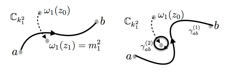
Figure 10: (left) pinch singularity (right) equivalent path $\gamma_{ab}\sim\gamma_{ab}^{1}+\gamma_{ab}^{2}$ with isolated pinch singularity

In order to motivate the Cutkosky rules we are going to sketch an argument given in the original paper [22] which is also reproduced in [1]. One considers an integral representation of the form

$$I(z)=\int dk_{1}^{2}\frac{F(k_{1}^{2},z)}{k_{1}^{2}-m_{1}^{2}-i0}\;,$$ (57)

where the variable $z$ is a function of the other momenta external and internal. Let the integrand $F$ contain a pole $w_{1}(z)$ which approaches $m_{1}^{2}$ for some $z$ such that there is going to be a pinch singularity as shown in Fig.10(left). One then switches to the equivalent configuration where the contour is deformed below the mass $m_{1}^{2}$ at the cost of encircling the singularity $m_{1}^{2}$. In the next step the integral is performed using Cauchy’s theorem which is equivalent to replacing the denominator by $\delta(k_{1}^{2}-m_{1}^{2})$. This argument falls short in justifying the additional physical condition $\theta((k_{1})_{0})$. Repeated use of the argument above, for each propagator gives the celebrated Cutkosky rules. The Cutkosky rules have recently been proven more rigorously [24] using ideas and methods by Pham. For the case of normal thresholds (unitarity cuts only) the method of the largest time equation [25] provides an elegant derivation of the cutting rules.

4.4 Anomalous Thresholds & physical Interpretation of Landau Equations

4.4.1 Brief remarks on anomalous Thresholds

By studying the $1$-loop bubble graph, in section 4.1, we have encountered singularities of the normal & pseudo and 2nd type; cf. Tab. 2. The most important singularities for practical purposes (e.g. dispersion relation, experiments) are the singularities which are on the physical sheet of which the normal one is the only type so far. This poses the questions whether there are any singularities on the physical sheet. By the work of Källén-Lehmann (11) we know that this is not the case for $2$-point function and we must therefore look at higher point functions.

There are indeed new classes of singularities for $3$- and higher point functions. A $3$-point function Fig. 11(right), for example, can be cut into more than two pieces which is going beyond the singularities discussed so far. Putting all three propagators on shell corresponds to $\alpha_{i}\neq 0$ at the level of the Landau equations. The corresponding singularities are known as anomalous thresholds. It is obvious that the singularities in say $p_{1}^{2}$ depend on the values of $p_{2}^{2}$ and $p_{3}^{2}$ (provided the line between the two is not contracted $\alpha_{1}\neq 0$ as otherwise one encounters the singularities discussed so far).

Whether or not anomalous thresholds appear on the physical sheet, returning to our original questions, depends on the external momenta $p_{1,2}^{2}$. Below we mention examples where the anomalous thresholds appear on the physical sheet.

• Consider the $1$-loop version of the $3$-point function with $p^{2}\equiv p_{2}^{2}=p_{3}^{2}$, $m\equiv m_{2}=m_{3}$ with masses as indicated in Fig. 11(left). For this configuration there is an anomalous threshold in $p_{1}^{2}\geq X$ with $X=4m^{2}-(p^{2}-(m^{2}+m_{1}^{2}))^{2}/m_{1}^{2}$ provided the condition $p^{2}>m^{2}+m_{1}^{2}$ holds [4]. $X$ is a branch point and the higher values are branch cuts. This anomalous threshold is below the two particle threshold at $4m^{2}$ and might be regarded as the very reason for calling these thresholds anomalous!

• For an example of a momentum configuration where the anomalous threshold is complex and on the physical sheet we refer the reader to the appendix in [26]. This anomalous threshold has to be taken into account in the dispersion relations by choosing the contour accordingly.

  The corresponding $3$-point function serves as an example where the Schwartz reflection principle (60) does not apply since the amplitude is imaginary on the entire real axis. In some more detail: the $1$-loop $3$-point function evaluated in PT does obey Schwartz’s reflection principle (60) with no anomalous threshold on the first sheet. It is though not the correct analytic continuation into the lower half-plane. Crucially, after elimination of an unphysical branch cut on the real line Schwartz’s reflection principle is not obeyed anymore allowing for the anomalous threshold to appear on the physical sheet in the lower half plane.

$$\begin{array}[]{l || l | l | l | l }\text{singularity}&\text{normal}&\text{pseudo}&\text{2nd type}&\text{anomalous}\\ \hline\cr\hline\cr\text{physical sheet}&\text{yes}&\text{no}&\text{no}&\text{$p_{2,3}^{2}$-dependent}\\ \text{remark}&\text{unitarity}&\text{ }&\text{mass-indep.}&\text{Leading Landau}\end{array}$$

Table 2: Different type of singularities described in the text: normal-, pseudo- & anomalous thresholds and 2nd type singularities. Whether or not the anomalous threshold is on the physical sheet depends on the momentum configuration of the other channels. E.g. in the example the triangle graph (cf. Fig. 11(right)) in the text the $p_{1}^{2}$-channels singularities are $p_{2,3}^{2}$-dependent. In addition to the singularities mentioned above there are also, the previously mentioned, mixed type singularities; mixed between 2nd type and others for different loop momenta. Not much is known about the Riemann sheet properties of mixed type singularities [1].

We end this section with a miscellaneous remarks on terminology and practicalities.

• Anomalous thresholds go beyond the concept of unitarity cuts in that they allow for cutting the diagram into more than two pieces. Cutkosky [22] was well aware of this and introduced the term generalised unitarity in the context of his equations.

• The number of propagators that are put on-shell (in a loop) give rise to a natural classification. The singularity with the maximal number of on-shell propagators (all $\alpha_{i}\neq 0\Rightarrow\det Q=0$) is usually referred to as the leading Landau singularity. In the case of the triangle diagram the anomalous threshold is the leading Landau singularity.

• When all but one external momenta are kept below the thresholds there are only normal thresholds on the physical sheet in the corresponding four momentum squared. For analytic computations this constitutes a method for obtaining correlation functions in a certain kinematic range. The remaining domain is then obtained by analytic continuation.

  For the assessment of dispersion relation, outside the range of concrete computations, this is not a practical method since one needs to know the location of all singularities on the physical sheet in order to choose a path $\gamma$ which does not cross any singularity.

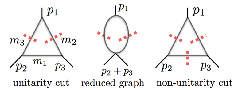
Figure 11: (left) normal threshold cut (non-leading singularity) (middle) the corresponding reduced graph for which $\alpha_{1}=0$ in the Landau equations. From the reduced graphs all lower singularities can be found. (right) the leading Landau singularity corresponding to a so called anomalous threshold (non-normal threshold)

4.4.2 Physical Interpretation of the second Landau Equations (46,47)

For physical momenta Coleman and Norton have given an interpretation of the second Landau equation [28]. It is found that (46,47) ensures that the corresponding diagram can occur as a real process where the Feynman-parameter $\alpha_{i}\sim\tau_{i}/m_{i}$ has the interpretation of being the proper time $\tau_{i}$ divided by the mass of the propagating particle.

This means that $\alpha_{i}=0$ corresponds to the case where the $i^{\rm th}$ particle does not propagate at all and gives the reduced graphs (e.g. Fig. 11(middle)) a more direct meaning. At last we note that the Coleman-Norton interpretation is a very reassuring result in view of the optical theorem’s (19) statemant that the discontinuity (related to singularities), of the forward scattering amplitude, originates from physical intermediate states.

5 Outlook

Even though dispersion relations are an old subject and a pure dispersive approach to particle physics has proven to be too complicated in practice, dispersion theory is and will remain a powerful tool in QFT as it follows from first principles and is intrinsically non-perturbative. This makes it particularly useful for hadronic physics which is not directly accessible by a perturbation expansion in the strong coupling constant. Dispersion relations are the most solid approach to quark hadron duality. Any approach to quark hadron duality should either start from or connect to dispersion relations.

In recent years dispersion relations and unitarity methods have also seen a major revival in evaluating perturbative diagrams (e.g. [29, 30, 31, 32] for reviews and applications). The bootstrapping programme has witnessed new exciting developments by limiting/fixing the target space functions of amplitudes. Old tools such as the Steinman relations, which are physical conditions on double discontinuities, have led to promising simplifications valid beyond perturbation theory [33].

Furthermore dispersion relations can serve to prove positivity, for example, when a physical quantity can be expressed as an unsubtracted dispersion integral with positive integrand (discontinuity). Examples are the so-called $c$- and $a$-theorems, which characterise the irreversibility of the renormalisation group flows in 2D and 4D. The dispersive proofs are given in [34, 35] in two and four dimensions by looking at two and four-point functions respectively. On another note, positivity of the Källén-Lehmann representation seemed to exclude the possibility of asymptotically free gauge theories in 1970 [36]. The Faddeev-Popov ghosts (negative metric) proved to be the loophole in this argument as they give rise to the negative sign of the $\beta$-function [37, 38].

I am grateful to James Gratrex for proofreading and to Einan Gardi for discussions on second type singularities. Apologies for all relevant references that were omitted. Last but not least I would like to thank the organisers of the “Strong Fields and Heavy Quarks” as well as the participants for a stimulating and pleasant atmosphere. I really did enjoy my trip to and around Dubna!

Appendix A The Schwartz Reflection Principle

Consider an analytic function $f(z)$ with $f(z)\in\mathbb{R}$ for $z\in I_{R}$ where $I_{R}$ is an interval on the real line. Then the following relation holds

$$f(z)=f(z^{*})^{*}\;,$$ (58)

which can be analytically continued to the entire plane. Note that analytic continuation is unique from any set with an accumulation point for which an interval is a special case. Hence Eq. (58) implies that

$${\rm Re}[f(z)]={\rm Re}[f(z^{*})]\;,\quad{\rm Im}[f(z)]=-{\rm Im}[f(z^{*})]\;.$$ (59)

Choosing $z=s+i0$ with $s\in\mathbb{R}$ it then follows that

$${\rm disc}[\Gamma(s)]=2i{\rm Im}[\Gamma(s)]\;,$$ (60)

which is a result known from experience with 2-point functions and intuitively in accordance with the optical theorem.

Appendix B Conventions

Here we summarise a few conventions. We are using the Minkowski metric of the form

$$g_{\mu\nu}={\rm diag}(1,-1,-1,-1)\;,$$ (61)

the following abbreviations for integrals over space and momentum space

$$\int_{x}=\int d^{4}x\;,\quad\int_{k}=\int d^{4}k\;,$$ (62)

and the relativistic state normalisation

$$\langle p|p^{\prime}\rangle=2E_{p}(2\pi)^{3}\delta^{(3)}(\vec{p}-\vec{p^{\prime}})\;,$$ (63)

where $E_{p}=\sqrt{\vec{p}^{2}+m^{2}}$ with $p=(E_{p},\vec{p})$.

References

- [1] R. Eden, D. Landshoff, P. Olive, and J. Polkinhorne, The analytic S-matrix. International Series In Pure and Applied Physics. McGraw-Hill, New York, 1966.
- [2] I. Todorov, Analytic Properties of Feynman Diagrams in Quantum Field Theory. Volume 38 in International Series of Monographs in Natural Philosophy. Elsevier, 1970.
- [3] G. Barton, Dispersion Techniques in Field Theory. 1965.
- [4] C. Itzykson and J. B. Zuber, Quantum Field Theory. International Series In Pure and Applied Physics. McGraw-Hill, New York, 1980. http://dx.doi.org/10.1063/1.2916419.
- [5] S. Weinberg, The Quantum theory of fields. Vol. 1: Foundations. Cambridge University Press, 2005.
- [6] E. de Rafael, “An Introduction to sum rules in QCD: Course,” in Probing the standard model of particle interactions. Proceedings, Summer School in Theoretical Physics, NATO Advanced Study Institute, 68th session, Les Houches, France, July 28-September 5, 1997. Pt. 1, 2, pp. 1171–1218. 1997. arXiv:hep-ph/9802448 [hep-ph].
- [7] S. S. Schweber, QED and the men who made it: Dyson, Feynman, Schwinger, and Tomonaga. 1994.
- [8] K. G. Wilson, “Nonlagrangian models of current algebra,” Phys. Rev. 179 (1969) 1499–1512.
- [9] R. Haag, “On quantum field theories,” Kong. Dan. Vid. Sel. Mat. Fys. Med. 29N12 (1955) 1–37. [Phil. Mag.46,376(1955)].
- [10] G. Kallen, “On the definition of the Renormalization Constants in Quantum Electrodynamics,” Helv. Phys. Acta 25 no. 4, (1952) 417. [,509(1952)].
- [11] H. Lehmann, “On the Properties of propagation functions and renormalization contants of quantized fields,” Nuovo Cim. 11 (1954) 342–357.
- [12] M. A. Shifman, A. I. Vainshtein, and V. I. Zakharov, “QCD and Resonance Physics. Theoretical Foundations,” Nucl. Phys. B147 (1979) 385–447.
- [13] T. DeGrand and C. E. Detar, Lattice methods for quantum chromodynamics. 2006.
- [14] M. Gell-Mann, M. L. Goldberger, and W. E. Thirring, “Use of causality conditions in quantum theory,” Phys. Rev. 95 (1954) 1612–1627.
- [15] S. Weinberg, “Precise relations between the spectra of vector and axial vector mesons,” Phys. Rev. Lett. 18 (1967) 507–509.
- [16] S. Weinberg, The quantum theory of fields. Vol. 2: Modern applications. Cambridge University Press, 2013.
- [17] G. Kallen and A. S. Wightman, The Analytic Properties of the Vacuum Expectation Value of a Product of Three Scalar Local Fields, vol. 1. 1958.
- [18] G. Kallen, “The analyticity domain of the four point function,” Nucl. Phys. 25 (1961) 568–603.
- [19] A. Martin, “The Rigorous analyticity unitarity program and its successes,” Lect. Notes Phys. 558 (2000) 127–135, arXiv:hep-ph/9906393 [hep-ph]. [,127(1999)].
- [20] E. Byckling and K. Kajantie, Particle Kinematics. University of Jyvaskyla, Jyvaskyla, Finland, 1971. http://www-spires.fnal.gov/spires/find/books/www?cl=QC794.6.K5B99.
- [21] L. D. Landau, “On analytic properties of vertex parts in quantum field theory,” Nucl. Phys. 13 (1959) 181–192.
- [22] R. E. Cutkosky, “Singularities and discontinuities of Feynman amplitudes,” J. Math. Phys. 1 (1960) 429–433.
- [23] M. E. Peskin and D. V. Schroeder, An Introduction to quantum field theory. 1995. http://www.slac.stanford.edu/spires/find/books/www?cl=QC174.45%3AP4.
- [24] S. Bloch and D. Kreimer, “Cutkosky Rules and Outer Space,” arXiv:1512.01705 [hep-th].
- [25] G. ’t Hooft and M. J. G. Veltman, “DIAGRAMMAR,” NATO Sci. Ser. B 4 (1974) 177–322.
- [26] M. Dimou, J. Lyon, and R. Zwicky, “Exclusive Chromomagnetism in heavy-to-light FCNCs,” Phys. Rev. D87 no. 7, (2013) 074008, arXiv:1212.2242 [hep-ph].
- [27] R. F. Streater and A. S. Wightman, PCT, spin and statistics, and all that. 1989.
- [28] S. Coleman and R. E. Norton, “Singularities in the physical region,” Nuovo Cim. 38 (1965) 438–442.
- [29] L. J. Dixon, “A brief introduction to modern amplitude methods,” in Proceedings, 2012 European School of High-Energy Physics (ESHEP 2012): La Pommeraye, Anjou, France, June 06-19, 2012, pp. 31–67. 2014. arXiv:1310.5353 [hep-ph]. https://inspirehep.net/record/1261436/files/arXiv:1310.5353.pdf.
- [30] H. Elvang and Y.-t. Huang, “Scattering Amplitudes,” arXiv:1308.1697 [hep-th].
- [31] J. M. Henn, “Lectures on differential equations for Feynman integrals,” J. Phys. A48 (2015) 153001, arXiv:1412.2296 [hep-ph].
- [32] E. Remiddi and L. Tancredi, “Differential equations and dispersion relations for Feynman amplitudes. The two-loop massive sunrise and the kite integral,” Nucl. Phys. B907 (2016) 400–444, arXiv:1602.01481 [hep-ph].
- [33] S. Caron-Huot, L. J. Dixon, A. McLeod, and M. von Hippel, “Bootstrapping a Five-Loop Amplitude from Steinmann Relations,” arXiv:1609.00669 [hep-th].
- [34] A. Cappelli, D. Friedan, and J. I. Latorre, “C theorem and spectral representation,” Nucl. Phys. B352 (1991) 616–670.
- [35] Z. Komargodski and A. Schwimmer, “On Renormalization Group Flows in Four Dimensions,” JHEP 12 (2011) 099, arXiv:1107.3987 [hep-th].
- [36] K. G. Wilson, “The Renormalization Group and Strong Interactions,” Phys. Rev. D3 (1971) 1818.
- [37] D. J. Gross and F. Wilczek, “Ultraviolet Behavior of Nonabelian Gauge Theories,” Phys. Rev. Lett. 30 (1973) 1343–1346.
- [38] H. D. Politzer, “Reliable Perturbative Results for Strong Interactions?,” Phys. Rev. Lett. 30 (1973) 1346–1349.