Finding Clustering Configurations to Accurately Infer Packet Structures from Network Data

Abstract

Clustering is often used for reverse engineering network protocols from captured network traces. The performance of clustering techniques is often contingent upon the selection of various parameters, which can have a severe impact on clustering quality. In this paper we experimentally investigate the effect of four different parameters with respect to network traces. We also determining the optimal parameter configuration with respect to traces from four different network protocols. Our results indicate that the choice of distance measure and the length of the message has the most substantial impact on cluster accuracy. Depending on the type of protocol, the $n$-gram length can also have a substantial impact.

1 Introduction

Protocol reverse-engineering (or protocol inference) is concerned with the challenge of inferring a specification of a network protocol specification from traces of network data. Inferred protocols can be valuable in a multitude of scenarios, especially in the contexts of security and testing. Inferred protocols can be used to derive novel test cases for black-box fuzzing [34, 1], can be used to interact with and explore botnets [6], or can be built into intrusion detection / supervisor frameworks [12].

A crucial step for any inference technique is to infer the packet structures from the data, so that it is possible to interpret a data stream as a sequence of packets. Most current approaches [4, 33, 13, 12, 36] identify common patterns within the data by way of an unsupervised Data Mining technique known as clustering [18]. Clustering can empirically elucidate the "natural", unknown and ideally interesting groups of messages within the captured network trace. These groups can then be used to identify the possible structures of message types implemented in the protocol.

Most network protocol inference techniques that involve clustering follow a common sequence of steps, but vary substantially in terms of the specific methods or parameters that they adopt with respect to clustering. For example, they might pre-process the data in different ways (e.g. limit messages to the first, 32 or 64 bytes, or fragment the message as $n$-grams). They might adopt different combinations of “distance measures”. They might be tailored towards text-based protocols or binary ones.

Most of the empirical results are presented with respect to a fixed configuration of clustering parameters. However, the sensitivity of clustering algorithms to their parameters [2] suggests that performance could vary significantly, depending on factors such as the type of protocol, the choice of distance measure, the amount of data, etc. Accordingly, this paper explores the following questions:

• RQ1 What is the effect of each variable on clustering accuracy?

• RQ2 What is the optimal configurations for clustering?

To answer the questions we have carried out an empirical study. This assesses the impact of four different parameters with respect to four real-world protocols. The chosen variables in the experimental study are: the length of the message, size of the sample, length of the $n$-gram (a message tokenisation approach used extensively by several applications), and the choice of distance measure (often required by clustering algorithms). The network protocols included in this study are: the Trivial File Transfer Protocol (TFTP), Domain Name Service (DNS), Server Message Block (SMB), and Hyper-Text Transfer Protocol (HTTP).

In this study, we have quantified the effect of each variable on clustering accuracy and have used this to identify an optimal configuration for clustering. Our results show that the choice of the distance measure have the largest effect on clustering accuracy, followed by the length of the message. Our results also indicate that combining the Ball-Hall internal clustering validation index with the Braun-Blanquet distance measure achieves results that are consistently better than other combinations.

2 Background and Motivation

In this section we begin with a general overview of protocol reverse engineering techniques. We then present the general sequence of steps that most approaches tend to adopt for clustering packet data. The section concludes with a discussion of the motivation of our work.

Network protocol specifications are the backbone of several security applications [31, 16, 5, 24, 22, 30]. Given an undocumented protocol (e.g., SMB, Skype), the goal of protocol reverse engineering is to extract the message format, which captures the structure of all messages that comprise the protocol, and the protocol state machine, which captures the valid sessions (message sequences) of the protocol. There are two common approaches for inferring protocol specifications: (1) by reverse engineering protocol implementations (e.g., sever-side analysis of executables while processing messages), or (2) by analysing network traffic. In this paper, we focus on the latter approach.

Figure 1: Common sequence of steps for network-based protocol reverse engineering.

2.0.1 Common Approach.

Figure 1 provides a high-level flow-chart of the the common sequence of steps that tend to be adopted by most traffic-based reverse engineering techniques to infer the message structure. Typically, the approach consists of following steps: traffic classification, message preprocessing, message clustering, and message alignment.

In the traffic classification step only messages that belong to target protocol are extracted for analysis. There are several ways to accomplish this task [22].

The message preprocessing step prepares protocol messages for clustering. This tends to involve data cleansing (e.g. filtering out irrelevant data) and dimensionality reduction [25] (reducing the number of features in terms of which the messages are to be clustered).

Typically, application protocols involve multiple different types of messages where each type has it own format. The clustering step serves to identify the possible types of these messages. This is achieved by partitioning the protocol messages into multiple distinct groups where messages in one cluster are of the same type following the same format.

Finally, The last step in the process is normally the message alignment step. Sequence alignment algorithms are often used (e.g., Needleman Wunsch algorithm [28]) to align protocol messages of the same type. The sequence alignment algorithm takes as input two similar protocol messages and align them, exposing the structural aspects of field similarities, differences, and gaps (if both messages have different lengths).

2.0.2 Motivation.

The common approach discussed above consists of multiple steps. Crucially, the choices that are made with respect to choosing the parameters for each of these steps can have a significant impact on the accuracy of the resulting inference results. The ideal choices may depend to an extent upon the characteristics of the network data (the amount of data available, the nature of the data (e.g. whether it is a text or binary protocol). Moreover, these factors are not independent; the effect of choosing a particular approach to tokenising the network data may be dependent on the choice of distance measure used to cluster the data, and might also depend on the amount and nature of the network data.

Choosing a suitable clustering configuration is ultimately a complex process. However, there is a dearth of guidance that can indicate how to choose different settings. Most protocol inference approaches are evaluated with respect to a static configuration. This is what motivates the work presented in this paper: to provide an experimental framework, along with some empirical data that can be used to guide the choice of suitable clustering configurations for packet extraction.

Figure 2: Experimental Framework for message clustering and validation

Therefore, it would be helpful if we could quantitatively assess how large or small the effect of those variables on clustering accuracy, and whether we could predict the best combination of these variables that enable us to achieve the best possible clustering.

3 A Modular Message Clustering Framework

In this section, we present a framework that enables us to provide answers to the above questions. The framework provides an intuitive, extensible basis for improving clustering and protocol inferencing in general. It takes the common stages outlined in Figure 1 and use to provide a controllable modular environment for clustering. This can be easily used to generate different message clustering configurations as compositions of various stages and parameters. Because we are especially interested in clustering (and steps lead up to clustering), we have integrated clustering validation step. This is to be able to evaluate clustering results and guide the inference process. The framework takes as input captured network messages and produces clustering validation scores.

The framework is shown in Figure 2 and explained in more detail below. Whenever a stage subject to parameter choices, these are listed in bold.

3.0.1 Traffic Classification.

The traffic classification method used in this step is the port-based method [22]. Port-based traffic classification relies upon the use of port numbers in the transport layer to filter network traffic. Typically, each protocol has standard port number(s) to represent that application of the protocol. We assume that the collected traffic is healthy (no malformed packets) and there is no misuse of port numbers, e.g. use of non-standard port numbers for communication [24].

3.0.2 Message Preprocessing.

We have divide the message preprocessing stage into the following steps:

Sample Manipulation.

This step accomplishes two tasks: First, to extract only data that belongs to the application layer protocol, i.e. data that belongs to the transport layer, network layer and link layer are discarded. Second, this step is also utilised to assign (manipulate) different sample sizes and message lengths according to different sizes and lengths. Parameters of this step: Sample Size & Message Length.

Message Tokenisation.

We use $n$-grams [8, 36] to tokenise protocol messages. An $n$-gram is a subsequence of $n$ consecutive characters from a longer sequence. The $n$-gram’s approach does not require protocol field delimiters to be predefined to the tokeniser. Normally, the result of this step is a large number of $n$-grams. The number of $n$-grams which can be generated from a message of length $m$ using an $n$-gram of length $n$ can be calculated from the following equation: $m-n+1$ where $(n\leq m)$. Parameters of this step: $N$-gram Length.

Feature Selection.

Messages from the same type normally have similar $n$-gram frequency distributions [36], therefore, we use the $n$-gram occurrences as a feature to distinguish between protocol messages (frequencies of the $n$-grams are counted in relation to their messages). To normalise the amount of contribution of each $n$-gram, we apply the Term Frequency-Inverse Term Frequency (TF/IDF) as a weighting scheme [32]. Also, we eliminate $n$-grams that carry no discriminative features. Since the generated feature space is mostly sparse, we remove $n$-grams which occur very infrequently (i.e. sparse $n$-grams); retaining only the common $n$-grams. We set the maximum sparseness allowed for $n$-grams to be retained to a certain percentage for the entire experiment.

3.0.3 Message Clustering.

In this step we cluster similar protocol messages into distinct clusters. We use an agglomerative hierarchical clustering algorithm with complete linkage clustering criteria [21]. Separate clusters are obtained by cutting the generated tree (dendrogram) at a given height. Throughout the experiment, we fix the cutting height to a certain level. Agglomerative hierarchical clustering requires a distance measure, the selected distance measures used for the experiment are explained in the evaluation section. Parameters of this step: Distance Measure.

3.0.4 Clustering Validation.

Clustering validation is the process of evaluating the result of a clustering algorithm. In general, cluster validation can be divided into two categories, external validation and internal validation. External validation measures require the actual "true" classes to be known a-priori. Internal measures evaluate the goodness of clustering based on internal geometrical aspects of the data (e.g., compactness and separation) without any external information.

We validate clustering results using external and internal clustering validation measures of choice. Through the external validation measure, clustering is validated by comparing the produced partitions from the clustering algorithm with the ground truth partitions. Instead of manually extracting message types from the formal documentations of the protocols, we use of-the-shelf network analyser that is capable of correctly parse the network traffic of the protocol to identify and label message types. We use tshark network analyser [38] (a command-line version of Wireshark) to automatically identify and extract true message labels to be provided to the external measure.

4 Evaluation

This section, consists of two parts. First, we present the experimental set-up that describes the experimental subjects and variables to be part of the experiment. The second part presents the methodology that will be used to answer the following research questions:

• RQ1 What is the effect of each variable on clustering accuracy?

• RQ2 What is the optimal variable configurations for clustering?

4.1 Experimental Set-up

4.1.1 Experimental Subjects.

The protocol traces included in the experiment are: the Trivial File Transfer Protocol (TFTP), the Domain Name Service (DNS), Server Message Block (SMB), and Hyper-Text Transfer Protocol (HTTP). The main datasets have been downloaded from a network security and monitoring website [29]. The selected protocols vary in terms of type of data (binary & text), and the complexity of their message structure. A summary of the collected network traces is provided in table 1.

4.1.2 Experimental Variables.

The constructed framework enables us to experiment with the following variables: length of the $n$-gram, length of the message, size of the sample, and choice of the distance measure. The four variables have always been key technical questions in the literature [13, 35, 37, 36].

• $N$-gram Length. We chose a range of values for the $n$-gram for each protocol trace. However, we have also observed the constraint indicated in equations 3.0.2 that the range should not exceed the length of the shortest message in the trace. A summary of the $n$-gram’s range for each protocol is shown in table 1 (column 4).

• Message Length. Three values are selected for the length of the message: 16 bytes, 32 bytes, and 64 bytes. We have experimented with different message lengths ranged from 3 bytes to 64 bytes, we have noticed that clustering scores, for all protocols, tend to be different and erratic when the length of the message is less than 12 bytes, and relatively similar when the length of the message lies between 12 to 16 bytes. We have also noticed that clustering scores gradually decline when the length of the message is greater than 16 bytes.

  Table 1: Summary of network traces and trace-dependant variables.

  Protocol	Sample Size	Type	Variable
  			$n$-gram	sub-sample
  TFTP	2300	Binary	2,3,4	500,1000,2000
  DNS	4000	Binary	2,3,4,5,6,7,8	1300,2600,3900
  SMB	1600	Mixed	2,3,4,5,6,7,8	500,1000,1500
  HTTP	1100	Text	2,3,4,5	300,600,900

• Sample Size. For each protocol, we have selected three three sub-samples from three different positions of the total sample while maintaining the order of the messages in each sub-sample. The size of each sub-sample is trace dependent and shown in table 1 (column 5).

• Distance Measure. With respect to distance measures, we use five distance measures, four measures are based on the similarity coefficients of the Jaccard index, Dice index, Braun-Blanquet index and the Cosine similarity index [32, 9] while the fifth is the Euclidean distance measure [19].

  For the similarity coefficients, the distance is defined as $D(a,b)=1-S(a,b)$, where $S$ is the similarity of two messages represented by $a$ and $b$ features respectively. The chosen distance measures are diverse and commonly used in the literature [32, 12, 37].

4.1.3 Clustering Validation Metrics.

We use the adjusted Rand index (aka corrected Rand) [20, 26] as the extrinsic measure. Typically, the score of the adjusted Rand index ranges from 0 to +1 where +1 indicates the two sets of clusters are identical and 0 when the two sets are completely independent. As for intrinsic validation measures, we use the Ball-Hall index [3], Calinski-Harabasz index [7], Davies-Bouldin index [14], Trace_WiB index [15], the SD index [18], and S_Dbw index [17].

The adjusted Rand index and internal validation indices are chosen based on popularity and recommendations by previous study [23]. We also ruled out internal measures that require intensive calculations.

4.2 Methodology

For each protocol trace, we use our framework to cluster protocol messages and validate the results through the extrinsic and intrinsic validation measures. The process is systematically executed using all possible combinations of variable values, and the clustering validation results are recorded each time.

4.2.1 RQ1. Measuring the Effect of Variables.

To measure the effect of each variable (e.g., choice of the $n$-gram ), we perform grouped statistical tests on the external validation scores (adjusted Rand). Because we cannot presume normality of the distribution of our data, we resort to non-parametric statistical tests. We use Cohen’s $d$ [10, 27] to measure the effect size.

The basic use of Cohen’s $d$ is to measure the mean difference (standardised) between two groups of adjusted Rand scores. Cohen’s $d$ is a pairwise test. We carry out every possible pairwise test for each variable (we compare the adjusted Rand scores for every pair of $n$-grams). Because we are mainly interested in the relative distance between variables and not the direction (which one was greater), we take the mean absolute value for all $d$’s to calculate the aggregate effect of the variable.

To be able to interpret the magnitude of $d$ for each test, Cohen nominated 0.2, 0.5 and 0.8 as the small, medium, and large reference values, respectively [10, 11]. However, Cohen urged researchers to interpret the effect size in the context of their experiments. He offered these reference values only as a "conventional frame of reference" which is recommended when no better basis is available. Typically, the magnitude (effect estimate) with the associated confidence interval (CI) are reported for each test. We use 95% as the confidence level for all the tests.

4.2.2 RQ2. Finding Optimal Variable Configurations.

To answer RQ2, we could simply refer to the highest score returned by the extrinsic measure and retrieve the corresponding variable values. However, in practice, message labels are often not available. Therefore, we use intrinsic validation measures. Since internal measures can be used to determine the optimal number of clusters [23], the general procedure to determine the optimal variable configurations is as follows:

• Step 1: For each protocol trace, use all possible variable combinations to get different clustering results.

• Step 2: Measure the clustering result obtained in step 1 using the corresponding internal validation index.

• Step 3: Choose the best validation result according to the criteria applied with the internal measure. (each internal validation measure has a rule which must be applied in order to obtain the optimal number of clusters).

• Step 4: Finally, we retrieve values of variables corresponding to the optimal number of clusters obtained in step 3.

5 Results

This sections presents the results of our experiment aiming at illustrating how various variables affect clustering and which configurations lead up to clustering with the highest score using the chosen internal validation measures.

5.0.1 RQ1. What is the effect of variables on clustering accuracy?

Figure 3 (a-d) shows Forest plots illustrating the effect of variables. The left-hand column lists the names of the variables and pairwise tests carried out between variable values. The right-column is a plot of these effects (shown as squares) within confidence intervals represented as horizontal lines. The overall effect of each variable is shown as a diamond. A vertical line indicating no-effect is also plotted.

The overall results show that the distance measure and the length of the message have a significant effect on clustering accuracy. Therefore, the choices of these variables are important. However, for TFTP, the choice of the $n$-gram seems to be the pivotal variable for clustering. The overall effect of the sample size is negligible. The results are explained in more detail below.

• Distance Measure. The effect of the distance measure on SMB & HTTP is significantly large. The overall effect is clearly visible in Figure 3 (c-d) as point estimates confidence intervals are shifted away from the no-effect line. The effect of the distance measure on TFTP & DNS is relativity less (medium). However, judging the precision of the estimated effects corroborated by the short confidence intervals, the effect is big enough to indicate the importance of the distance measure for all protocols.

• Message Length. For DNS & HTTP, the average effect of the message’s length is greater than one std. (standard deviation) which is very large for both protocols, while the effect on SMB is about 0.5 std. (medium). For the TFTP protocol, the message length does not seem to have any effect on clustering, this is clearly indicated in Figure 3 (a) as all effect estimates lie on the no-effect line.

• $N$-gram Length. The effect of the $n$-gram on DNS, SMB and HTTP ranges from small to medium. However, Figure 3 (b&c) indicate that the effect of this variable is much more significant for the DNS & SMB protocols than the HTTP as clearly shown by the individual tests as well as the overall effect of the variable. As for TFTP, the effect of the $n$-gram is critically (large) with 3.08 standard deviation. Therefore, length of the $n$-gram is important choice.

• Sample Size. The overall effect of the sample size is negligible. For all protocols, this is clearly evident that the effect of this variable lies within wider confidence intervals and all of these confidence intervals intersect with the no-effect line which indicates that sample size as a whole has insignificant impact on clustering.

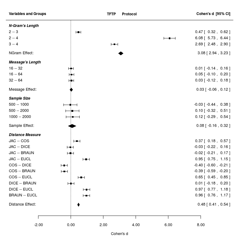
(a) TFTP

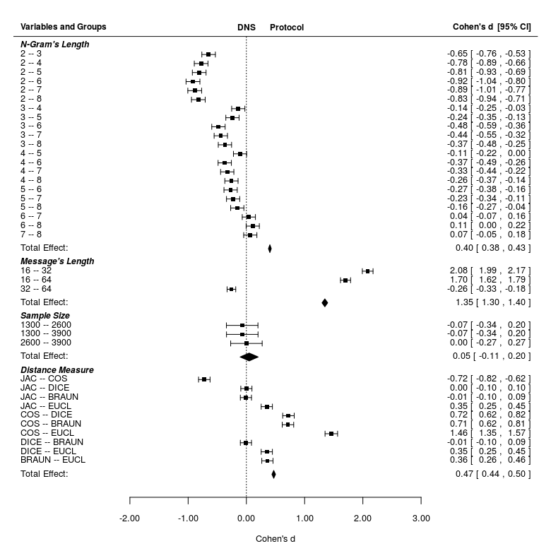
(b) DNS

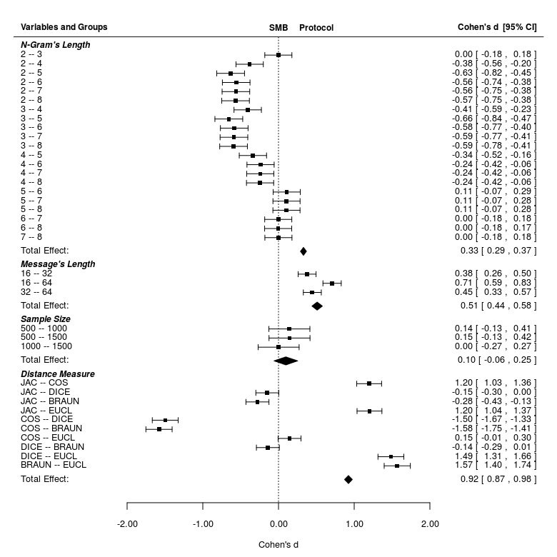
(c) SMB

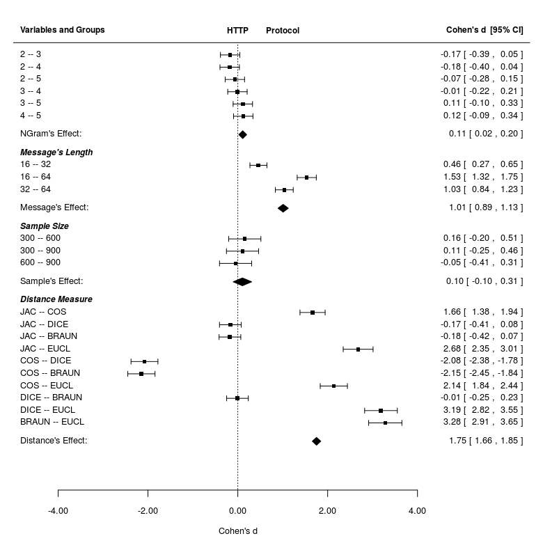
(d) HTTP

Figure 3: Forest plots showing the effect of variables on clustering accuracy. The figures show the estimated effects of the pairwise tests on the adjusted Rand scores between variable values as well as the aggregate affect of each variable. It also, shows the corresponding 95% confidence intervals for each test.

5.0.2 RQ2: What is the optimal variable configurations for clustering?

In general, the results show that the combination of the Ball-Hall validity index and the Braun-Blanquet binary similarity measure tend to give the best results in predicting the optimal variable configuration for clustering.

The results are shown in Table 2d (a-d). The table shows the experimental variables and chosen internal measures as well the the score of the adjusted Rand corresponding to each internal measure. For TFTP and DNS, the Ball-Hall index has predicted the best variable combination (clustering score) as indicated in Table 2d (a-b), while the SD and Calinski-Harabasz indices have predicted the best variable combination for SMB and HTTP protocols respectively with the Ball-Hall index comes the second.

Also, Table 2d (a-d) shows internal measures tend to give better predictions with the binary similarity measures of Braun-Blanquet, Dice & Jaccard.

Table 2: Performance of internal validation measures in predicting optimal variable configuration for clustering.

Distance	Sample	$n$-gram	Message	adj. Rand	Internal Measure
Jaccard	200	2	16	0.998782	Trace_WiB
	2300	2	16	0.998254	Ball_Hall
	100	3	16	0.938577	SD_Dis
	1500	4	16	0.000214	Calinski_Harabasz
	1500	4	16	0.000214	Davies_Bouldin
	1100	4	16	0.000131	S_Dbw
Dice	200	2	16	0.998782	Trace_WiB
	2300	2	32	0.998254	Ball_Hall
	100	3	16	0.938577	SD_Dis
	1500	4	16	0.000214	Calinski_Harabasz
	1500	4	16	0.000214	Davies_Bouldin
	1100	4	16	0.000131	S_Dbw
Braun-Blanquet	2300	2	32	0.999982	Ball_Hall
	2300	2	32	0.999982	Trace_WiB
	100	3	16	0.938577	SD_Dis
	1500	4	16	0.000214	Calinski_Harabasz
	1500	4	16	0.000214	Davies_Bouldin
	1100	4	16	0.000117	S_Dbw
Cosine	1100	3	16	0.945071	S_Dbw
	800	2	64	0.629911	Trace_WiB
	100	2	16	0.104278	SD_Dis
	1700	4	64	0.003506	Ball_Hall
	1500	4	16	0.000214	Calinski_Harabasz
	1500	4	16	0.000214	Davies_Bouldin
Euclidean	100	4	32	0.314674	Ball_Hall
	2100	3	32	0.015229	S_Dbw
	1200	4	32	0.000971	Trace_WiB
	800	4	16	0.000610	SD_Dis
	2200	4	16	0.000230	Calinski_Harabasz
	1500	4	16	0.000000	Davies_Bouldin

(a) TFTP

Distance	Sample	$n$-gram	Message	adj. Rand	Internal Measure
Jaccard	4000	7	16	0.989203	Ball_Hall
	4000	4	16	0.531224	Calinski_Harabasz
	200	4	16	0.344495	SD_Dis
	2300	2	16	0.111911	Davies_Bouldin
	100	2	16	0.072107	S_Dbw
	800	2	32	0.019798	Trace_WiB
Dice	4000	7	16	0.989203	Ball_Hall
	4000	4	16	0.531224	Calinski_Harabasz
	200	4	16	0.344495	SD_Dis
	2300	2	16	0.111911	Davies_Bouldin
	100	2	16	0.072107	S_Dbw
	800	2	32	0.019798	Trace_WiB
Braun-Blanquet	4000	7	16	0.989203	Ball_Hall
	4000	4	16	0.531224	Calinski_Harabasz
	200	4	16	0.344495	SD_Dis
	2300	2	16	0.189199	Davies_Bouldin
	400	2	16	0.077443	Trace_WiB
	100	2	16	0.072107	S_Dbw
Cosine	4000	6	16	0.945626	Ball_Hall
	3600	3	32	0.346439	Trace_WiB
	300	8	16	0.297692	SD_Dis
	400	2	16	0.134757	S_Dbw
	4000	2	16	0.116275	Davies_Bouldin
	4000	2	32	0.044579	Calinski_Harabasz
Euclidean	2300	8	16	0.233399	Calinski_Harabasz
	1900	8	16	0.211938	SD_Dis
	800	7	16	0.175221	Trace_WiB
	300	3	64	0.027146	Ball_Hall
	3400	3	16	0.012933	S_Dbw
	100	2	32	0.000000	Davies_Bouldin

(b) DNS

Distance	Sample	$n$-gram	Message	adj. Rand	Internal Measure
Jaccard	100	5	16	1.000000	SD_Dis
	100	4	64	0.992056	Trace_WiB
	1600	3	16	0.180173	Ball_Hall
	1600	5	32	0.002438	Calinski_Harabasz
	1600	3	32	0.002438	S_Dbw
	100	2	64	0.000000	Davies_Bouldin
Dice	100	5	16	1.000000	SD_Dis
	100	4	64	0.710890	Trace_WiB
	1600	3	16	0.180173	Ball_Hall
	1600	5	32	0.002438	Calinski_Harabasz
	1600	3	32	0.002438	S_Dbw
	100	2	64	0.000000	Davies_Bouldin
Braun-Blanquet	100	5	16	1.000000	SD_Dis
	1600	4	32	0.747453	Ball_Hall
	100	4	64	0.710890	Trace_WiB
	1600	2	16	0.002438	Calinski_Harabasz
	1600	2	16	0.002438	S_Dbw
	100	2	64	0.000000	Davies_Bouldin
Cosine	100	5	16	0.271637	SD_Dis
	200	8	16	0.158804	Calinski_Harabasz
	200	8	16	0.158804	Davies_Bouldin
	200	8	16	0.158804	S_Dbw
	300	5	16	0.047732	Ball_Hall
	1000	4	16	0.003836	Trace_WiB
Euclidean	1600	7	64	0.000000	Ball_Hall
	400	2	16	0.000000	Calinski_Harabasz
	100	2	16	0.000000	Davies_Bouldin
	700	2	16	0.000000	SD_Dis
	1200	7	16	0.000000	S_Dbw
	200	2	16	0.000000	Trace_WiB

(c) SMB

Distance	Sample	$n$-gram	Message	adj. Rand	Internal Measure
Jaccard	1000	5	16	0.941975	Calinski_Harabasz
	900	5	16	0.941237	S_Dbw
	1100	4	16	0.924386	Ball_Hall
	100	5	16	0.821678	SD_Dis
	1100	5	32	0.448247	Trace_WiB
	700	3	64	0.335951	Davies_Bouldin
Dice	1000	5	16	0.941975	Calinski_Harabasz
	900	5	16	0.941237	S_Dbw
	1100	4	16	0.924386	Ball_Hall
	100	5	16	0.821678	SD_Dis
	700	3	64	0.471805	Davies_Bouldin
	100	2	64	0.238019	Trace_WiB
Braun-Blanquet	1000	5	16	0.942082	Calinski_Harabasz
	1100	4	16	0.902149	Ball_Hall
	100	5	16	0.821678	SD_Dis
	100	2	16	0.764644	S_Dbw
	700	3	64	0.453987	Davies_Bouldin
	100	4	64	0.403513	Trace_WiB
Cosine	800	4	16	0.465563	Calinski_Harabasz
	100	3	16	0.431648	Ball_Hall
	100	3	16	0.431648	Davies_Bouldin
	200	3	16	0.362845	S_Dbw
	100	5	16	0.355834	SD_Dis
	100	2	32	0.192357	Trace_WiB
Euclidean	1000	5	16	0.311167	Calinski_Harabasz
	700	3	16	0.274333	S_Dbw
	100	3	16	0.145950	Ball_Hall
	100	5	32	0.030939	SD_Dis
	100	2	64	0.000000	Davies_Bouldin
	100	4	64	0.000000	Trace_WiB

(d) HTTP

6 Threats to Validity

Although all experiments were tested on exactly the same machine and under the same experimental configurations, threats to external validity might arise which might limit the generalisability of these findings.

• Representative Protocols. Since we our study involved only four network protocols, they may not be representative of the entire family of network protocols . However, this threat is partially considered by selecting the possible types of network protocols (text & binary protocols).

• Representative Traces. Some of the collected network traces are relatively small in size and may not be representative of the protocol under study. The effect of some of the variables for the TFTP protocol vary from the rest of the protocols (DNS,SMB & HTTP), this is could be due to the fact that the gathered messages are not well trained to be representative of the protocol behaviour (lack of diversity of traffic seen in the trace).

7 Conclusions and Future Work

In this paper, we investigated the impact of four important variables on clustering accuracy as part of reverse engineering protocols from network traces. To support our investigation, we have developed a modular framework that enables us to produce arbitrary clustering configurations of protocol inferencing. We have applied this framework to data traces from four widely used network protocols. Our research indicates the following:

• The choice of the distance measure and length of the message is of paramount importance for clustering.

• The number of messages in the trace does not have significant impact on clustering accuracy.

• It is possible to derive highly accurate clustering configurations without relying upon labelled examples (i.e., by using internal validation measures).

In the future, we plan to mitigate threats to validity by incorporating more diverse network protocols. We also plan to enrich our protocol inference by integrating clustering internal validation to predict optimal configurations for clustering.

References

- [1] Aarts, F., Kuppens, H., Tretmans, J., Vaandrager, F., Verwer, S.: Improving active mealy machine learning for protocol conformance testing. Machine learning 96(1-2), 189–224 (2014)
- [2] Anderberg, M.R.: Cluster Analysis for Applications. Academic Press (1973)
- [3] Ball, G., Hall, D.: Isodata: A novel method of data analysis and pattern classification. Tech. rep., Stanford Research Institute (1965)
- [4] Beddoe, M.A.: Network protocol analysis using bioinformatics algorithms. http://www.4tphi.net/ awalters/PI/PI.html (2004), http://www.4tphi.net/~awalters/PI/PI.html
- [5] Caballero, J., Kang, M.G., Venkataraman, S., Song, D., Poosankam, P., Blum, A.: Fig: Automatic fingerprint generation. In: In 14th Annual Network and Distributed System Security Conference (NDSS (2007)
- [6] Caballero, J., Poosankam, P., Kreibich, C., Song, D.: Dispatcher: enabling active botnet infiltration using automatic protocol reverse-engineering. In: Proceedings of the 16th ACM conference on Computer and communications security (2009)
- [7] Calinski, T., Harabasz, J.: A dendrite method for cluster analysis. Communications in Statistics-Simulation and Computation 3(1), 1–27 (1974)
- [8] Cavnar, W.B., Trenkle, J.M.: N-gram-based text categorization. In: In Proceedings of SDAIR-94, 3rd Annual Symposium on Document Analysis and Information Retrieval. pp. 161–175 (1994)
- [9] Choi, S.S., Cha, S.H., Tappert, C.: A Survey of Binary Similarity and Distance Measures. Journal on Systemics, Cybernetics and Informatics 8(1), 43–48 (2010)
- [10] Cohen, J.: Statistical Power Analysis for the Behavioral Sciences. New York:Academic Press, 2nd ed. edn. (1988)
- [11] Cohen, J.: Quantitative methods in psychology: A power primer. Psychological Bulletin 112(1), 155–159 (1992)
- [12] Comparetti, P.M., Wondracek, G., Kruegel, C., Kirda, E.: Prospex: Protocol specification extraction. In: Proceedings of the 2009 30th IEEE Symposium on Security and Privacy (2009)
- [13] Cui, W., Kannan, J., Wang, H.J.: Discoverer: automatic protocol reverse engineering from network traces. In: Proceedings of 16th USENIX Security Symposium on USENIX Security Symposium (2007)
- [14] Davies, D.L., Bouldin, D.W.: A cluster separation measure. IEEE Trans. Pattern Anal. Mach. Intell. 1(2), 224–227 (Feb 1979)
- [15] Friedman, H., Rubin., J.: On some invariant criteria for grouping data. Journal of he American Statistical Associations, 62:1159-1178 (1967)
- [16] Greene, M.S.A., Amini, P.: Fuzzing: Brute Force Vulnerability Discovery. Addison-Wesley (2007)
- [17] Halkidi, M., Vazirgiannis, M.: Clustering validity assessment: finding the optimal partitioning of a data set. In: Data Mining, 2001. ICDM 2001, Proceedings IEEE International Conference on (2001)
- [18] Halkidi, M., Batistakis, Y., Vazirgiannis, M.: On clustering validation techniques. J. Intell. Inf. Syst. 17(2-3), 107–145 (Dec 2001)
- [19] Han, J., Kamber, M., Pei, J.: Data Mining: Concepts and Techniques. Morgan Kaufmann Publishers Inc. (2011)
- [20] Hubert, L., Arabie, P.: Comparing partitions. Journal of Classification 2(1), 193–218 (1985)
- [21] Jain, A.K., Dubes, R.C.: Algorithms for Clustering Data. Prentice-Hall, Inc. (1988)
- [22] Kim, H., Claffy, K., Fomenkov, M., Barman, D., Faloutsos, M., Lee, K.: Internet traffic classification demystified: Myths, caveats, and the best practices. In: Proceedings of the 2008 ACM CoNEXT Conference (2008)
- [23] Liu, Y., Li, Z., Xiong, H., Gao, X., Wu, J.: Understanding of internal clustering validation measures. In: Data Mining (ICDM), 2010 IEEE 10th International Conference on (2010)
- [24] Ma, J., Levchenko, K., Kreibich, C., Savage, S., Voelker, G.M.: Unexpected means of protocol inference. In: Proceedings of the 6th ACM SIGCOMM conference on Internet measurement (2006)
- [25] Maimon, O., Rokach, L.: Data Mining and Knowledge Discovery Handbook. Springer-Verlag New York, Inc., Secaucus, NJ, USA (2005)
- [26] Meilă, M.: Comparing clusterings: an information based distance. J. Multivar. Anal. (2007)
- [27] Myers L., W.D., F., L.: Research Design and Statistical Analysis. Routledge, 3rd ed. edn. (2010)
- [28] Needleman, S.B., Wunsch, C.D.: A general method applicable to the search for similarities in the amino acid sequence of two proteins. Journal of Molecular Biology 48(3), 443–453 (1970)
- [29] NETRESEC: Network forensics and network security monitoring. http://www.netresec.com/ (2016), http://www.netresec.com/
- [30] Pang, R., Paxson, V., Sommer, R., Peterson, L.: binpac: a yacc for writing application protocol parsers. In: Proceedings of the 6th ACM SIGCOMM conference on Internet measurement (2006)
- [31] Paxson, V.: Bro: a system for detecting network intruders in real-time. Comput. Netw. 31(23-24), 2435–2463 (Dec 1999)
- [32] Rieck, K., Laskov, P.: Linear-time computation of similarity measures for sequential data. J. Mach. Learn. Res. 9, 23–48 (Jun 2008), http://dl.acm.org/citation.cfm?id=1390681.1390683
- [33] Shevertalov, M., Mancoridis, S.: A reverse engineering tool for extracting protocols of networked applications. In: Reverse Engineering, 2007. WCRE 2007. 14th Working Conference on. pp. 229–238 (2007)
- [34] Walkinshaw, N., Bogdanov, K., Derrick, J., Paris, J.: Increasing functional coverage by inductive testing: a case study. In: Testing Software and Systems, pp. 126–141 (2010)
- [35] Wang, Y., Li, X., Meng, J., Zhao, Y., Zhang, Z., Guo, L.: Biprominer: Automatic mining of binary protocol features. In: Proceedings of the 2011 12th International Conference on Parallel and Distributed Computing, Applications and Technologies. pp. 179–184. PDCAT ’11, IEEE Computer Society, Washington, DC, USA (2011), http://dx.doi.org/10.1109/PDCAT.2011.25
- [36] Wang, Y., chun Yun, X., Shafiq, M.Z., Wang, L., Liu, A.X., Zhang, Z., Yao, D., 0002, Y.Z., Guo, L.: A semantics aware approach to automated reverse engineering unknown protocols. In: ICNP. pp. 1–10. IEEE (2012)
- [37] Wang, Y., Zhang, Z., Yao, D.D., Qu, B., Guo, L.: Inferring protocol state machine from network traces: a probabilistic approach. In: Proceedings of the 9th international conference on Applied cryptography and network security. pp. 1–18. ACNS’11, Springer-Verlag, Berlin, Heidelberg (2011), http://dl.acm.org/citation.cfm?id=2025968.2025970
- [38] WireShark: tshark:dump and analyze network traffic. https://www.wireshark.org/docs/man-pages/tshark.html (2004), https://www.wireshark.org/docs/man-pages/tshark.html