Decision Tree Classification on Outsourced Data

Abstract

This paper proposes a client-server decision tree learning method for outsourced private data. The privacy model is anatomization/fragmentation: the server sees data values, but the link between sensitive and identifying information is encrypted with a key known only to clients. Clients have limited processing and storage capability. Both sensitive and identifying information thus are stored on the server. The approach presented also retains most processing at the server, and client-side processing is amortized over predictions made by the clients. Experiments on various datasets show that the method produces decision trees approaching the accuracy of a non-private decision tree, while substantially reducing the client’s computing resource requirements.

1 Introduction

Data publishing without revealing sensitive information is an important problem. Many privacy definitions have been proposed based on generalizing/suppressing data ($l$-diversity[21], k-anonymity [28] [29], t-closeness [20]). Other alternatives include value swapping [23] and noise addition (e.g., differential privacy [8]). Generalization consists of replacing identifying attribute values with a less specific version [4]. Suppression can be viewed as the ultimate generalization, replacing the identifying value with an “any” value. [4]. These approaches have the advantage of preserving truth, but a less specific truth that reduces the utility of the published data.

Xiao and Tao proposed anatomization as a method to enforce $l$-diversity while preserving specific data values[32]. Anatomization splits tuples across two tables, one containing identifying information and the other containing private information. The more general approach of fragmentation [5] divides a given dataset’s attributes into two sets of attributes (2 partitions) such that an encryption mechanism avoids associations between two different small partitions. Vimercati et al. extend fragmentation to multiple partitions [6], and Tamas et al. propose an extension that deals with multiple sensitive attributes [10]. The main advantage of anatomization/fragmentation is that it preserves the original values of data; the uncertainty is only in the mapping between individuals and sensitive values.

There is concern that anatomization is vulnerable to several prior knowledge attacks [16], [12]. While this can be an issue, any method that provides any meaningful utility fails to provide perfect privacy against a sufficiently strong adversary [8]. Legally recognized standards such as the so-called “Safe Harbor” rules of the U.S. Healthcare Insurance Portability and Accountability Act (HIPAA) [13] allow release of data that bears some risk of re-identification; the belief is that the greater good of beneficial use of the data outweighs the risk to privacy.

This paper does not attempt to resolve that issue (although we use a randomized rather than optimized grouping that provides resistance to the type of attacks above.) Instead, this paper attempts to develop a simple and efficient decision tree learning method from an ${l}$-diverse dataset which satisfies ${l}$-diversity in anatomization. The developed decision tree is embedded into a recent client-server database model [25, 24].

The database model is a storage outsourcing mechanism that supports anatomization. In this database model, the client is the owner of the data and stores the data at the server in an ${l}$-diverse anatomy scheme. The server provides some query preprocessing that reduce client’s workload. The model proposed by Nergiz et al. has four significant aspects relevant to this paper [25, 24]: 1) a given data table (or dataset) of a client is split into two partitions, a sensitive table (single sensitive attribute) and an identifier table (multiple identifying or quasi-identifying attributes). 2) A join key is stored with the data, but encrypted with a key known only to the client, preventing the server from associating a sensitive value with the correct identity. 3) There is also an unencrypted group-level join key allowing the server to map a group of identifiers with a group of sensitive attributes, these groups are $l$-diverse. 4) The server can use this group information to perform some query processing (or in the case of this paper, tree learning), reducing the client effort needed to get final results. The reader is advised to visit [24, 25] for further details and performance aspects of Nergiz et al.’s database model.

This paper investigates whether it is possible to learn a decision tree in the above database model with minimal client resource usage. We assume that the client has limited storage and processing resources, just enough to make small refinements on any model learned at the server. The remainder of this paper refers to the server of Nergiz et al.’s client-server database model as a cloud database server (CDBS). Terms “CDBS” and “server” are used interchangeably.

1.1 Related Work

There have been studies in how to mine anonymized data. Fung et al. [9] give a top-down specialization method (TDS) for anonymization so that the anonymized data allows accurate decision trees. Chui et al. [3] and Leung et al. [18] address the frequent itemset mining problem. Ngai et al. proposes a clustering algorithm that handles the anonymized data as uncertain information [26]. Kriegel et al. propose a hierarchical density based clustering method using fuzzy objects [17]. Xiao et al. discusses the problem of distance calculation for uncertain objects [31]. Nearest Neighbor classification using generalized data is investigated by Martin [22]. Zhang et al. studies Naive Bayes using partially specified data [33]. Dowd et al. studies decision tree classifier with random substitutions [7]. Kantarcioglu et al. proposes a new Support Vector classification and Nearest Neighbor classification that deals with anonymized data [14]. They extend the generalization based anonymization scheme to keep all necessary statistics and use these statistics to build effective classifiers. Freidman et al. investigate learning C4.5 decision trees from datasets that satisfy differential privacy [27]. Jagannathan et al. propose a tree classifier based on random forests that is built from differentially private data [15].

These methods are all based on generalization/suppression or noise addition techniques. Anatomized data provides additional detail that has the potential to improve learning, but also additional uncertainty that must be dealt with. In addition, the database model of [25, 24] provides exact matching information that can be extracted only at the client; providing additional opportunities to improve learning.

Another approach related to mining anatomized data in the client-server database model is vertically partitioned data mining (e.g., [11, 30]). Vertically partitioned data mining makes strong assumptions about data partitions and what data can be shared, and typically assume that each party holding data has significant computational power. For example, some decision tree techniques assume that two tuples of two partitions can be linked directly to each other, that the tuples are ordered in the same way; and that the class labels are known for both partitions. In one sense, our problem is easier, as one party (client) can see all the data. However, we assume this party (again client) does not have the resources to even store all the data, much less to build the tree.

1.2 Contributions

The model of [25] would allow a client to construct an exact decision tree by downloading the identifier and sensitive tables of a dataset (or data table), decrypting the join key, and joining the identifying and sensitive information (rebuilding the original dataset). The remainder of this paper will use terms dataset and data table interchangeably. The goal of this paper is to reduce resource requirements at the client, by doing as much work as possible at the server. The challenge is that the server is not allowed to know exact mappings between identifying and sensitive information (and server can’t know without background knowledge these mappings due to $l$-diversity of anatomization scheme).

We assume that the class attribute is not the sensitive attribute, as effectively learning this at the server implies a de-facto violation of $l$-diversity. However, predicting values that fall into identifying information (e.g., predicting geographic location given other demographics and a disease) does not necessarily face this difficulty. We thus perform processing involving identifying attributes at the server. The client then needs only do the necessary processing to utilize the sensitive attribute to complete the tree.

The key novelty is that this final processing is:

1. Performed only when a prediction would make use of that information, and

2. The cost is amortized over many predictions.

The resource requirements (including memory, CPU cost, and communications) remain relatively low per prediction, thus allowing this to be performed on lightweight clients that are assumed to have limited storage capabilities.

We first give a set of definitions and define a prediction task for anatomized data. We then detail our method, along with cost and privacy discussions. Section 4 shows performance with experiments on various UCI datasets. The performance evaluation includes execution time, memory requirement and classification accuracy. We conclude the paper with a brief summary and future directions.

2 Definitions and Prediction Task

We give a set of definitions that are required to explain our work, and use them to define the prediction task for anatomized data.

Definition 1.

A dataset ${D}$ is called person specific dataset for population ${P}$ if each tuple ${t\in D}$ belongs to a unique individual ${p\in P}$.

The person specific dataset ${D}$ has ${A_{1},\cdots,A_{d}}$ identifier attributes and a sensitive attribute ${A_{s}}$. We use ${D.A_{i}}$ to refer to the $i$th attribute of a person specific dataset ${D}$. Similarly, we use ${t.A_{i}}$ to refer to the $i$th attribute of a tuple in a person specific dataset ${D}$ (either ${1\leq i\leq d}$ or ${i=s}$ holds).

Definition 2.

A group ${G_{j}}$ is a subset of tuples in dataset ${D}$ such that ${D=\cup_{j=1}^{m}G_{j}}$, and for any pair ${(G_{j1},G_{j2})}$ where ${1\leq i\neq j\leq m}$, ${G_{j1}\cap G_{j2}=\emptyset}$.

Definition 3.

A set of groups is said to be l-diverse if and only if for all groups ${G_{j}}$ ${\forall v\in\pi_{A_{s}}G_{j},\frac{freq(v,G_{j})}{|G_{j}|}\leq\frac{1}{l}}$ where ${A_{s}}$ is the sensitive attribute in ${D}$, ${freq(v,G_{j})}$ is the frequency of ${v}$ in ${G_{j}}$ and ${|G_{j}|}$ is the number of tuples in ${G_{j}}$.

We define anatomy as in [24, 25].

Definition 4.

Given a person specific dataset ${D}$ partitioned in m groups using l-diversity without generalization, anatomy produces a identifier table ${IT}$ and a sensitive table ${ST}$ as follows. ${IT}$ has schema

${(A_{1},...,A_{d},GID,ESEQ)}$

where ${A_{i}\in I_{T}}$ for ${1\leq i\leq d=|I_{T}|}$, ${I_{T}}$ is the set of identifying attributes in ${D}$, ${GID}$ is the group id of the group and ${ESEQ}$ is the encryption of a unique sequence number, ${SEQ}$. For each ${G_{j}\in D}$ and each tuple ${t\in G_{j}}$ (with sequence number ${s}$), ${IT}$ has a tuple of the form:

${(t.A_{1},...,t.A_{d},j,E_{k}(salt,s))}$

The ST has schema

${(SEQ,GID,A_{s})}$

where ${A_{s}}$ is the sensitive attribute in ${D}$, ${GID}$ is the group id of the group and ${SEQ}$ is a (unique but randomly ordered) sequence number for that tuple in ${ST}$, used as an input for the ${ESEQ}$ of the corresponding tuple in ${IT}$. For each ${G_{j}\in D}$ and each tuple ${t\in G_{j}}$, ${ST}$ has a tuple of the form:

${(s,j,t.A_{s})}$

The reason why the anatomy definition [32] is extended in [24, 25] and in this paper is that CDBS operations like selection, insertion, deletion etc. require the consideration of the (encrypted where necessary) sequence number. The sequence number is in fact used to rebuild the original mapping between the identifying attributes and the sensitive attributes of a given tuple (cf. Section 1). The sequence numbers and encrypted sequence numbers are created during the splitting phase of an outsourced table (cf. Section 1). Here is a brief explanation of how this mechanism works in several database operations:

Firstly, $ESEQ$ field values in the identifying table are decrypted by the client to find the true sequence number of given tuples. Secondly, the true sequence number values in the identifying table is equi-joined with the sequence number $SEQ$ field values in the sensitive table. The database has some sequence numbers in the sensitive table $ST$ which are same as the true sequence numbers (this is guaranteed in the initial splitting phase, see Section 1). The original tuples are eventually rebuilt after this equi-join operation. The reader is directed to [24, 25] for further issues about CDBS design. In this paper, we will use sequence number values to do client-side refinement of the decision tree.

Definition 5.

An l-diverse group G is said to have a simple l-diverse distribution if

${\forall p\in G}$ and ${\forall v\in\pi_{A_{s}}G_{j},P(p.A_{s}=v)=\frac{(freq(v,G_{j}))}{|G_{j}|}}$

where ${p}$ denotes an individual and ${A_{s}}$, ${freq(*)}$ are as in Definition 3.

Definition 6.

A person specific dataset ${D}$ has simple l-diverse distribution if for every group ${G_{i}\in D}$ where ${1\leq i\leq m}$ holds, ${G_{i}}$ has a simple l-diverse distribution according to Definition 5.

This paper focuses on collaborative decision tree learning between the client and CDBS. Next, we define the principal components of the collaborative decision tree.

Definition 7.

Given two partitions ${IT}$ and ${ST}$ of a person specific dataset ${D}$, a base decision tree (BDT) is a decision tree classifier that is built from ${A_{1},\cdots,A_{d}}$ attributes ${(I_{T})}$. Given a BDT that has leaves $Y$; every leaf ${y\in Y}$ has tuples in the following format:

${(t.A_{1},\cdots,t.A_{d},j,E_{k}(salt,s))}$

${j,E_{k}(salt,s)}$ fields are ignored when the BDT is learned. Note that the BDT maintains the simple $l$-diverse distribution which is the privacy constraint of CDBS. Given a leaf ${y\in Y}$, each tuple ${t\in y}$ is equally likely to match${l}$ different values of ${A_{s}}$. The privacy issues with the base decision tree are discussed in the next section.

Definition 8.

Given a base decision tree ${BDT}$, the leaves ${Y\in BDT}$; a leaf ${y\in Y}$ is called a refined leaf if and only if it points to a sub-tree rooted at ${y}$ that is encrypted (using symmetric key encryption).

We will elaborate in the privacy discussion of the next section how and why a base decision tree has encrypted sub-trees.

Definition 9.

Given a base decision tree ${BDT}$, the leaves ${Y\in BDT}$; a leaf ${y\in Y}$ is called unrefined leaf if and only if it doesn’t point to a sub-tree rooted at ${y}$.

In the remainder of this paper, ${Y}$ is used to note the leaves of a decision tree.

We finish the discussion in this section by defining the prediction task of our classifier. The prediction task is to predict an identifying attribute (${A_{i}\in I_{T}}$) given other identifying attributes (${A_{j}}$ satisfying ${1\leq i\neq j\leq d}$) and the sensitive attribute (${A_{s}}$).

A real life example would be learning from patient health records. The U.S. Healthcare laws protect individually identifiable health information [1]. An anatomized database, while it contains individually identifiable information, does not link this directly to the (sensitive) health information. Suppose we have public directory information as identifying attributes including zipcode, gender, age, as well as specific identifiers such as name (which are presumably uninteresting for building a decision tree.) We also have a sensitive table consisting of diagnosis. Suppose the goal was to identify locations where people with particular backgrounds (including health conditions) live, through learning a decision tree with class value location. While this seems a somewhat contrived example, it would likely have identified the infamous Love Canal district[19] as an unusually common location for those with the diagnosis birth defect.

3 Anatomization Decision Trees

We investigate three possible approaches to build decision trees from anatomized data in Nergiz et al.’s client-server database model. We call this family of decision trees as anatomization decision trees, because they are all built from anatomized data. Each approach differs according to how ${IT}$ and ${ST}$ tables are used.

In the discussion of anatomization decision trees, algorithms that require encryption are assumed to use AES-128 symmetric key encryption. We first discuss two baseline approaches: pure-client side learning, and pure server-side learning. Section 3.2 explains the collaborative decision tree learning. We finally compare collaborative decision tree learning with the baselines in Section 3.3.

3.1 Baseline Approaches: CDBS Learning and Client Naïve Learning

The baseline approaches compose two different scenarios for learning. The first scenario is that the CDBS learns a base decision tree using only the ${IT}$ partition of dataset ${D}$ (cf. Section 2). The second scenario is that client learns a decision tree using the person specific dataset ${D}$ retrieved from the CDBS. We call the first learning scenario CDBS learning and the second learning scenario client naïve learning.

In client naïve learning, the client retrieves the person specific dataset $D$ by getting all the tuples in the respective $IT$ and $ST$ partitions of $D$. $IT$ and $ST$ partitions are joined together using the join key and the non-anatomized set of records in dataset ${D}$ is obtained (cf. Sections 1 and 2). The client learns decision tree from this non-anatomized set of records in dataset $D$. In other words, the client rebuilds from its outsourced data the non-anatomized version (original version) of dataset $D$ and learns the decision tree itself without any attribute uncertainty. Client naïve learning brings up some vital issues and respective solutions below:

The privacy aspect of the decision tree is an issue. The client learns the decision tree from the non-anatomized version of ${D}$, so the identifying attributes and the sensitive attribute are associated in the decision tree. The client has to store this model at the CDBS (limited storage resource assumption, see Section 1), but since the model is built from non-anatomized dataset, it may reveal information violating privacy constraints (particularly in conjunction with the anatomized data). The solution is to encrypt the decision tree and to store the encrypted tree at CDBS.

Encrypting the decision tree raises the issue of how to make an inference of the class label for a new instance. The CDBS cannot make the inferences because the stored tree is encrypted. This leads to the following approach: each time the class label of a new tuple is predicted, the client retrieves the encrypted decision tree, decrypts the encrypted decision tree and makes the prediction. This makes the inference phase quite expensive for the client in client naïve learning.

The other extreme is CDBS learning: the server constructs a base decision tree using only the identifying information. Base decision tree makes the prediction operation very easy and low cost for the client. Given a predicted tuple ${t_{p}}$ and a base decision tree for predicting class label ${A_{c}\in I_{T}}$; the client just deletes the attribute field ${t_{p}.A_{s}}$ (an ${O(1)}$ time operation). Then, it sends the rest of the tuple ${t_{p}}$ to the CDBS and CDBS makes the tree inference. The client has ${O(1)}$ inference cost and network overhead. This low cost for client is the main advantage of CDBS learning. The drawback of CDBS learning is that the base decision tree ignores the sensitive attribute. This is not a big drawback if ${A_{s}}$ is a weak predictor of the class label. On the other hand, the base decision tree’s accuracy is likely to be low if ${A_{s}}$ is a strong predictor of the class label.

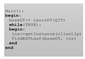
Figure 1: Collaborative Learning Main Function (Called by Server)

3.2 Collaborative Decision Tree Learning

One way to mitigate the drawbacks of CDBS learning and client naïve learning is the usage of grouping statistics among anatomy groups of the person specific dataset ${D}$. Grouping statistics are the distribution of ${A_{s}}$ among anatomy groups ${G_{i}}$ provided that ${1\leq i\leq m}$ and ${\cup_{m}G_{i}=D}$ hold. Grouping statistics might have the potential to determine an interesting decision tree split for a class label ${A_{i}\in I_{T}}$. However, to avoid correlation-based attacks, we assume the insertion operation of CDBS is designed to create groups randomly while satisfying the simple $l$-diverse distribution [25]. It is unlikely to find an interesting pattern for split using group statistics.

This paper proposes a new collaborative decision tree algorithm involving CDBS and client collaboration. Given a dataset ${D}$ partitioned on ${IT}$ and ${ST}$, $IT$ and $ST$ partitions stored on CDBS, a class label ${A_{i}\in I_{T}}$; CDBS initiates building the collaborative decision tree. First, the server builds a base decision tree. Then, the base decision tree leaves ${Y}$ are improved by the client. For every leaf ${y\in Y}$, the improvement is a sub-tree learned by the client. The client uses the tuples in leaf ${y}$ to learn an improved sub-tree. Figures 1, 2 and 3 give pseudo code of the collaborative decision tree learning process.

Figure 1 shows the Main() function that is called by CDBS to initiate collaborative learning. The LearnDT(IT) function call builds the base decision tree from the $IT$ partition. The client improvements on the base decision tree are made on the fly when doing predictions. To make a prediction, a tuple ${(ins.A_{1},\cdots,}$ ${ins.A_{i-1},ins.A_{i+1},\cdots,ins.A_{d})}$ is sent to the CDBS. The getInstance() function call receives the sent tuple ins (cf. Figure 1). FindBDTLeaf(baseDT, ins) function is called by CDBS for every predicted tuple ins once the predicted tuple ins is received by getInstance() calls (cf. Figure 1).

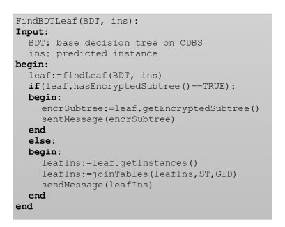
Figure 2: Collaborative Learning FindBDTLeaf Function (Called by Server)

The FindBDTLeaf function essentially finds the appropriate base decision tree leaf ${y\in Y}$ for the client to complete (if not already done) and sends leaf $y$ to the client (cf. Figure 2). Given tuple ins and the base decision tree baseDT, the findLeaf(BDT,ins) function call finds the correct leaf ${y\in Y}$ using a usual decision tree inference with attribute values ${(ins.A_{1},\cdots,ins.A_{i-1},}$ ${ins.A_{i+1},\cdots,ins.A_{d})}$. Then, FindBDTLeaf verifies if ${y}$ points to an encrypted sub-tree that was previously learned by a client (if statement in pseudocode). (The subtree is encrypted to ensure privacy constraints are satisfied, this will be discussed in more detail later.) If ${y}$ points to an encrypted sub-tree, it sends the client the encrypted sub-tree as a response message (sentMessage(encrSubTree) function call). Otherwise, CDBS sends the tuples belonging to ${y}$ by function call sentMessage(leafIns).

All tuples ${t\in y}$ are partitioned across ${IT}$ and ${ST}$ on CDBS. Reconstructing the original tuples $t\in y$ is done on the client side (Inference() function call, cf. Figure 3, explained later). The joinTables(leafIns, ST, GID) function call prepares the message leafIns including the following tuples: leafIns include every tuple ${t\in y}$ with all combinations of $l$ sensitive attributes. In other words function joinTables() matches every tuple $t\in y$ with all $l$ potential sensitive attributes using the $GID$ field as the join key (a group-level join, giving all possible tuples given the l-diverse dataset, not just the true matching values). The explanation of Inference() function will clarify why this join operation is done (cf. Figure 3).

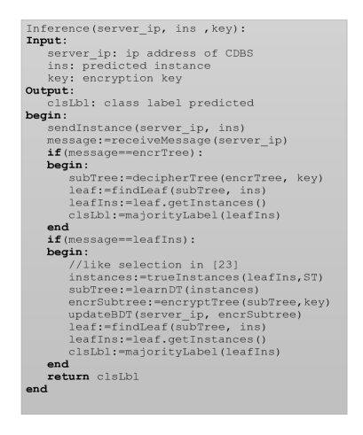
Figure 3: Collaborative Learning Inference Function (Called by Client)

A client calls the Inference() function to make predictions or on the fly improvements (cf. Figure 3). The client sends a predicted tuple ins to the CDBS using the sendInstance() function. It receives the message sent by function FindBDTLeaf() using receiveMessage(). As mentioned in the FindBDTLeaf() discussion, the message can be either an encrypted sub-tree (encrTree) or tuples $t$ of leaf $y$ (leafIns). leafIns is in fact all tuples $t\in y$ such that every tuple $t$ is matched with all $l$ potential sensitive attribute values. If the message is an encrypted sub-tree (encrTree), Inference() just decrypts the encrypted sub-tree using decipherTree() function, finds the appropriate leaf $y^{\prime}$ as in regular tree inference using findLeaf() function and predicts the class label of tuple ins by taking majority of the class labels in $y^{\prime}$ using majorityLabel() function. If message is leafIns, the Inference() function reconstructs the non-anatomized leaf instances (instances) from leafIns: it decrypts the encrypted sequence numbers $ESEQ$ in identifying attributes of leafIns to find true sequence numbers and eliminates the tuples $t$ of leafIns that don’t have the sensitive table sequence numbers $SEQ$ the same as true sequence numbers. trueInstances() function does the former operation. We discussed earlier in Section 2 how this sequence number fields are designed and how they are used in Nergiz et al.’s client server database model [24, 25]. Inference() learns a sub decision tree (subTree) from instances using learnDT() function, encrypts subTree (encryptTree() function call) and sends subTree back to CDBS for updating as we discussed earlier in FindBDTLeaf(). Finally, Inference() finds the appropriate leaf $y^{\prime}$ as in regular tree inference using findLeaf() function and predicts the class label of tuple ins by taking majority of the class labels in $y^{\prime}$ using majorityLabel() function.

We finish the discussion in this subsection by considering the encryption of the client’s improved sub-trees. Encryption is necessary due to privacy concerns. Once the sub-tree is built, it has leaves having tuples in ${(t.A_{1},\cdots,t.A_{d},t.A_{s})}$ format. Moreover, the sub-tree also has splits with the true values of ${A_{s}}$. Thus, whole sub-tree should be encrypted so that no additional information regarding the correlation between tuples and sensitive values is provided to the CDBS when the sub-tree is stored. The symmetric key encryption of sub-tree preserves the privacy of person specific dataset $D$ according to following theorem.

Theorem 1.

(Privacy Preserving Learning): Given a person specific dataset ${D}$ on CDBS having a simple $l$-diverse distribution, the collaborative decision tree learning preserves the simple $l$-diverse distribution of ${D}$.

Proof.

Given a snapshot ${IT(i)}$ and ${ST(i)}$ of ${D}$ on CDBS at time $i$, suppose that a collaborative decision tree is learned using the algorithm in Figures 1–3. CDBS learns the associations within the identifying attributes (Figure 1). The CDBS is allowed to learn such associations according to its privacy definition [24] [25]. These associations do not provide any background information linking identifying attributes and sensitive attribute. The Client learns all associations within identifying attributes and the sensitive attribute (cf. Figure 3), but no additional information is provided back to the server (except in encrypted form.) The simple $l$-diverse distribution is maintained for snapshots ${IT(i)}$, ${ST(i)}$ at ith time. The inference operation at jth time (${1\leq i\leq j\leq\infty}$) is done with CDBS and client. The base decision tree has only associations between identifying attributes, so the CDBS part of inference is safe. The encrypted sub-trees are used on client side of inference, so assuming semantically secure encryption this gives no further information to the CDBS. Throughout predictions, some base decision tree leaves might never be visited, but this only discloses that certain identifying information has not come up for prediction. This is not a disclosure case about sensitive information. CDBS cannot know whether the sensitive attribute has a better information for the unvisited leaves’ tuples as sensitive attributes’ positive/negative correlation or uncorrelation with identifying attributes would not be known without any background knowledge. The encrypted subtrees of visited leaves do not let CDBS learn this kind of correlation information. Consequently, collaborative decision tree learning preserves the simple l-diverse distribution in inference at time ${j}$. ∎

Our privacy analysis doesn’t include the case where there are multiple clients that outsource different data. The reader might be concerned that if there are multiple clients who outsource their data in anatomization format, some clients’ identifying information can be other clients’ sensitive information. This cross correlation might create privacy concerns about the whole client-server database model. This is an issue dealt in the original Nergiz et al.’s client-server database model [25, 24]. Since we have shown that our decision tree learning reveals no additional information, it cannot result in privacy violations provided the underlying database does not violate privacy constraints.

3.3 Cost Discussion

It is difficult to estimate a practical average cost savings for collaborative decision tree learning, as it depends not only on the data, but on the client’s memory, processing, and communication resources.

If the identifying attributes are bad predictors, the base decision tree will be complex. A complex decision tree model means that it has many splits yielding small leaves, requiring only a small amount of client memory and computation during the prediction phase. The client needs to build more complex sub-trees to achieve good prediction. However, small leaves means that the cost per sub-tree will be small, even though the total cost (amortized over many predictions) is high. If the identifying attributes are good predictors, the base decision tree will be simple. A tree having few splits will yield fewer, but larger leaves. This increases the cost for the first prediction, but also increases the likelihood that future predictions will hit an already completed subtree.

In either case, the client requires less memory than client naïve learning, as it needs to hold at most the tuples that reach a leaf, along with all possible sensitive values for those tuples. The next theorem gives an upper bound for collaborative decision tree learning cost under reasonable assumptions and feasible alternatives.

Theorem 2.

(Cost Upper Bound) Given a person specific dataset ${D}$, ${IT}$ and ${ST}$ partitions on CDBS storing ${D}$, similar number of splits in base decision tree, client improvement sub-trees and client naïve learning tree; the client cost of collaborative decision tree learning cannot be bigger than client naïve learning’s cost.

Proof.

Assume that ${D}$ is ${O(n\times m)}$ where ${n}$ is the number of rows and ${m}$ is the number of attributes. Let us also assume that the client cost of collaborative decision tree learning is bigger than the client naïve learning cost. Given a base decision tree with ${O(m)}$ leaves, depth, and split (worst case tree type); the total cost of base decision tree learning is ${O(nm^{2})}$. This cost is excluded in client cost since it is not executed by the client. Given a client sub-tree on the $i$th base decision tree leaf (${n_{i}}$ is number of rows) with ${O(m)}$ splits, leaves and depth (same as base decision tree); the cost of learning a sub-tree is ${O(n_{i}m^{2})}$. The total cost of collaborative decision tree learning is ${O(\sum_{i}n_{i}m^{2})}$ which is ${O(nm^{2})}$ (${1\leq i\leq m}$). Given client naïve learning’s resulting model with ${O(m)}$ splits, leaves and depth (same as base decision tree); the total client cost is ${O(nm^{2})}$. Client naïve learning has a client cost that is equal to the collaborative decision tree learning’s client cost. This result contradicts to the basic assumption. Thus, collaborative decision tree learning cost cannot be bigger than client naïve learning cost by contradiction. ∎

The same theorem can be developed for encryption, decryption and network costs as well (intrinsic). The number of splits assumption in the cost theorem is a worst case assumption for cost calculation. In practice, the sub-tree on the ith leaf of the base decision tree will be much simpler (have fewer splits) than both the base decision and client naïve learning trees. Client sub-trees would be learned from less data and less data yields the simple subtrees having fewer splits. Fewer splits mean low training, inference, encryption/decryption and network costs for client in collaborative decision tree learning.

4 Experiments

We now compare our collaborative decision tree learning (cdtl) with the client naïve (cnl) and CDBS learning (cdbsl) on four datasets from the UCI collection: adult, vote, autos and Australian credit. We evaluate two things: The classification accuracy (presumably better than clbs, but worse than client naïve), and the cost for those performance improvements.

The Adult dataset is composed of US census data. An individual’s income is the class attribute (more than 50K vs less than 50K). It has 48842 tuples where each tuple has 15 attributes. The Vote dataset contains 485 tuples where each tuple has 16 binary attributes. An attribute is the vote of a senator in a session. A senator’s party affiliation is the class attribute (democrat vs republican). The Autos datasets contains 205 tuples where each tuple has 26 attributes. The class label is either symboling (risk rating) or price of a car. Autos dataset’s continuous attributes are discretized in our experiments and a binary class label is created from price of a car (low price vs. high price). The Australian credit dataset has 690 tuples where each tuple has 16 attributes. The class attribute is whether a credit application is approved or not (${+}$ vs. ${-}$). We chose these four because they are large enough to demonstrate performance differences, and reasonably challenging for decision tree learning. The reader is advised to visit [2] to learn more about the structure of the datasets.

Experiments 1 and 2 are made on auto and vote datasets respectively, because they can simulate a real world example of $l$-diverse data. While privacy may not be a real issue for this data, we give an examples below that we feel are a reasonable simulation of a privacy-sensitive scenario. (True privacy-sensitive data is hard to obtain and publish results on, precisely because it is privacy-sensitive.) Experiment 1 uses attribute symboling (risk rating) as the sensitive attribute and predicts the attribute price. Suppose that there is a dealership outsourcing their cars’ pricing data. Clients might not want to buy some of their cars because of high risk factor (high insurance premium), so $l$-diversity is preserved for symboling. Experiment 2 is done on the vote dataset. It sets physician fee-freeze as the sensitive attribute. Suppose that senate’s voting records are outsourced to a cloud database. Voting records in public sessions are available and they can be used with party affiliation to identify a senator’s identity. Thus, the voting records of a private session should be l-diverse.

Experiments 3 and 5 are made on the Australian credit dataset and adult dataset. Decision tree models fit well on these datasets. These experiments show how the cdtl models behave when the underlying data is convenient for decision tree learning. Experiment 3 uses Australian credit dataset. It assigns attribute A9 as sensitive attribute and predicts the class attribute. Experiment 4 uses the adult dataset. It assigns attribute relationship as sensitive attribute and predicts the class attribute. Relationship and A9 are the strongest predictors of class labels in adult and Australian credit datasets. Experiment 4 and 5 measure together the effect of the sensitive attribute’s predictor power given a fixed dataset. In experiment 5, the adult dataset is used again with sensitive attribute age that is a moderate predictor. Experiments 4 and 5 use the tuples which belong to individuals in non-private work class. So, the experiments are made on a subsample of 14936 tuples.

On each experiment, we apply cdbsl, cnl, cdtl with 10-fold cross validation. We measure accuracy, memory savings and execution time savings. Weka J48 is used for decision tree learning with reduced error pruning. 20% of the training sets are used for reduced error pruning. Given a training/test pair of 10-fold cross validation, the prune set is chosen randomly once so that cdbsl, cnl, cdtl models are compared within the same model space (same pruning set and training set for each algorithm). The experiments on vote and australian credit datasets learn binary decision trees whereas the experiments on auto and adult datasets learn non-binary decision trees. Experiments are done using a physically remote cloud server; and a laptop with Intel i5 processor and 4 GB RAM. Internet connection speed was 100 Mbps.

$$ets=\frac{cdtl\,execution\,time}{cnl\,execution\,time}$$ (1)

$$ms=\frac{cdtl\,memory\,requirement}{cnl\,memory\,requirement}$$ (2)

Equations 1 and 2 calculate execution time savings (ets) and memory savings (ms) respectively in the experiments. Savings are maximized as both formulas approach to zero. In contrary, savings are minimized as both formulas approach 1. Execution times (Eq. 1) include client’s encryption/decryption, network and learning/inference costs on a training set and test set pair (ith iteration of cross validation). In equation 2, the number of tuples in training set is the cnl’s memory requirement whereas the number of tuples in the base decision tree’s (BDT) biggest leaf is the cdtl’s memory requirement. Since the client learns sub-trees on the fly from the unrefined leaves, the biggest leaf is the memory upper bound.

Figure 4 and Figure 5 provides box plots showing elapsed time and memory savings measurements on each of the 10 folds. Cdbsl is not shown, as the client cost is 0. The blue dots on the boxplots show the mean time and memory savings. Savings graphs exhibit visually the tradeoff between ms and ets. Given a dataset, if the memory savings are high, the time requirements are low (as expected.) It is expected since the high ms indicates a complex base decision tree model in cdtl. The client needs to do more improvement in cdtl since the leaf provided is already a bad predictor. In addition, high ms and low ets can lead to complex decision trees that can produce overfitting. On the other hand, low ms indicate a simple base decision tree in cdtl. Little remains to be done at the client since the leaf provided is already a good predictor.

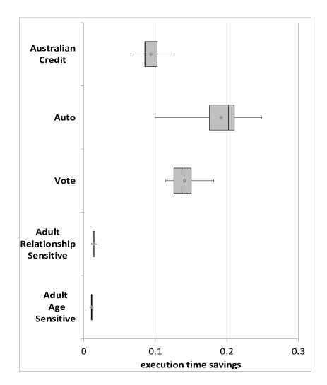
Figure 4: Execution Time Savings Graph

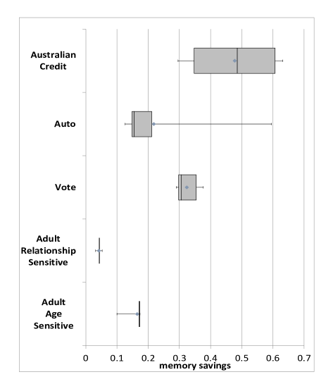
Figure 5: Memory Savings Graph

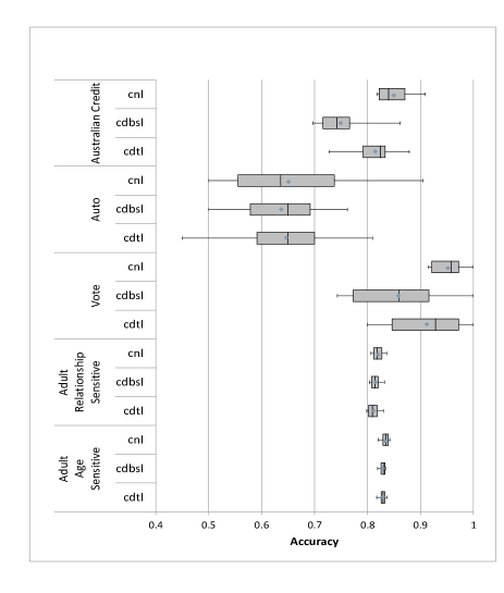
Figure 6: Accuracy Graph

Figure 6 provides measured prediction accuracies in the experiments. On average, the cnl decision trees have the best accuracy, as expected. Cdbsl decision trees have the worst accuracy and cdtl decision trees is generally somewhere between. This accuracy trend is expected since cdbsl gives a decision tree which is essentially the same as the base decision tree in cdtl. So, cdtl’s accuracy values show the effect of client improvements which are done to the cdbsl model. The exception is in experiment 4 (the Adult dataset). The sensitive attribute is not a very good predictor. This exceptional case shows that the collaborative model becomes too complex after client improving (overfitting). Execution time savings and memory savings graphs justify this fact (Figs. 5 and 6). A possible solution to avoid cdtl overfitting is memory savings threshold (threshold for BDT leaf size on CDBS). However, it is hard to define an exact threshold value. Given a fixed training set on CDBS, cdtl can be learned with various BDT thresholds. The threshold having the best accuracy on the pruning set can be chosen and client improvements can be applied on this model.

5 Conclusion

This paper proposes a decision tree learning method for outsourced data in an anatomization scheme. A real world prediction task is defined for anatomization. Collaborative decision tree learning (cdtl), which uses cloud database server (CDBS) and client, is studied to achieve this prediction task. Cdtl is proven to preserve the privacy of data provider. Cdtl is tested on various datasets and the results show that fairly accurate decision trees can be built whereas client’s learning and inference costs are reduced remarkably.

The next challenge is to extend this work in a new framework such that there is no client processing while accurate decision trees are learned. Another direction is to observe how the collaborative decision tree learning algorithm performs relative to the recent differential privacy decision trees.

6 Acknowledgments

We wish to thank to Dr. Qutaibah Malluhi and Dr. Ryan Riley for their helpful comments throughout the preparation of this work. We also wish to thank to Qatar University for providing physical facilities required for experimentation. This publication was made possible by NPRP grant 09-256-1-046 from the Qatar National Research Fund. The statements made herein are solely the responsibility of the authors.

References

- [1] The health insurance portability and accountability act of 1996. Technical Report Federal Register 65 FR 82462, Department of Health and Human Services, Office of the Secretary, Dec. 2000.
- [2] A. Asuncion and D. Newman. UCI machine learning repository, 2007.
- [3] C.-K. Chui, B. Kao, and E. Hung. Mining frequent itemsets from uncertain data. In Proceedings of the 11th Pacific-Asia conference on Advances in knowledge discovery and data mining, PAKDD’07, pages 47–58, Berlin, Heidelberg, 2007. Springer-Verlag.
- [4] V. Ciriani, S. De, C. Vimercati, S. Foresti, and P. Samarati. Chapter 1 k-anonymous data mining: A survey.
- [5] V. Ciriani, S. D. C. D. Vimercati, S. Foresti, S. Jajodia, S. Paraboschi, and P. Samarati. Combining fragmentation and encryption to protect privacy in data storage. ACM Trans. Inf. Syst. Secur., 13:22:1–22:33, July 2010.
- [6] S. D. C. di Vimercati, S. Foresti, S. Jajodia, G. Livraga, S. Paraboschi, and P. Samarati. Extending loose associations to multiple fragments. In DBSec’13, pages 1–16, 2013.
- [7] J. Dowd, S. Xu, and W. Zhang. Privacy-preserving decision tree mining based on random substitutions. Technical report, In International Conference on Emerging Trends in Information and Communication Security, 2005.
- [8] C. Dwork. Differential privacy. In 33rd International Colloquium on Automata, Languages and Programming (ICALP 2006), pages 1–12, Venice, Italy, July 9-16 2006.
- [9] B. C. M. Fung, K. Wang, and P. S. Yu. Top-down specialization for information and privacy preservation. In Proceedings of the 21st International Conference on Data Engineering, ICDE ’05, pages 205–216, Washington, DC, USA, 2005. IEEE Computer Society.
- [10] T. Gal, Z. Chen, and A. Gangopadhyay. A privacy protection model for patient data with multiple sensitive attributes. International Journal of Information Security and Privacy, IGI Global, Hershey, PA, 2(3):28–44, 2008.
- [11] C. Giannella, K. Liu, T. Olsen, and H. Kargupta. Communication efficient construction of decision trees over heterogeneously distributed data. In In Proceedings of The Fourth IEEE International Conference on Data Mining (ICDM’04, pages 67–74, 2004.
- [12] X. He, Y. Xiao, Y. Li, Q. Wang, W. Wang, and B. Shi. Permutation anonymization: Improving anatomy for privacy preservation in data publication. In L. Cao, J. Z. Huang, J. Bailey, Y. S. Koh, and J. Luo, editors, PAKDD Workshops, volume 7104 of Lecture Notes in Computer Science, pages 111–123. Springer, 2011.
- [13] Standard for privacy of individually identifiable health information. Federal Register, 67(157):53181–53273, Aug. 14 2002.
- [14] A. Inan, M. Kantarcioglu, and E. Bertino. Using anonymized data for classification. In Proceedings of the 2009 IEEE International Conference on Data Engineering, ICDE ’09, pages 429–440, Washington, DC, USA, 2009. IEEE Computer Society.
- [15] G. Jagannathan, K. Pillaipakkamnatt, and R. N. Wright. A practical differentially private random decision tree classifier. Transactions on Data Privacy, 5(1):273–295, 2012.
- [16] D. Kifer. Attacks on privacy and de finetti’s theorem. In In SIGMOD, 2009.
- [17] H.-P. Kriegel and M. Pfeifle. Hierarchical density-based clustering of uncertain data. In Proceedings of the Fifth IEEE International Conference on Data Mining, ICDM ’05, pages 689–692, Washington, DC, USA, 2005. IEEE Computer Society.
- [18] C. K.-S. Leung and D. A. Brajczuk. Efficient algorithms for mining constrained frequent patterns from uncertain data. In Proceedings of the 1st ACM SIGKDD Workshop on Knowledge Discovery from Uncertain Data, U ’09, pages 9–18, New York, NY, USA, 2009. ACM.
- [19] A. G. Levine. Love canal: Science, politics and people. Lexington, MA, 1982. D.C. Heath and Company.
- [20] N. Li and T. Li. t-closeness: Privacy beyond k-anonymity and l-diversity. In Proceedings of the 23nd International Conference on Data Engineering (ICDE ’07), Istanbul, Turkey, Apr. 16-20 2007.
- [21] A. Machanavajjhala, J. Gehrke, D. Kifer, and M. Venkitasubramaniam. -diversity: Privacy beyond -anonymity. In Proceedings of the 22nd IEEE International Conference on Data Engineering (ICDE 2006), Atlanta Georgia, Apr. 2006.
- [22] B. Martin. Instance-based learning : Nearest neighbor with generalization. Technical report, 1995.
- [23] R. A. Moore, Jr. Controlled data-swapping techniques for masking public use microdata sets. Statistical Research Division Report Series RR 96-04, U.S. Bureau of the Census, Washington, DC., 1996.
- [24] A. E. Nergiz and C. Clifton. Query processing in private data outsourcing using anonymization. In The 25th IFIP WG 11.3 Conference on Data and Applications Security and Privacy (DBSEC-11), Richmond, Virginia, July 11-13 2011.
- [25] A. E. Nergiz, C. Clifton, and Q. Malluhi. Updating outsourced anatomized private databases. In 16th International Conference on Extending Database Technology (EDBT), Genoa, Italy, Mar. 18-22 2013.
- [26] W. K. Ngai, B. Kao, C. K. Chui, R. Cheng, M. Chau, and K. Y. Yip. Efficient clustering of uncertain data. In Proceedings of the Sixth International Conference on Data Mining, ICDM ’06, pages 436–445, Washington, DC, USA, 2006. IEEE Computer Society.
- [27] B. Rao, B. Krishnapuram, A. Tomkins, and Q. Yang, editors. Proceedings of the 16th ACM SIGKDD International Conference on Knowledge Discovery and Data Mining, Washington, DC, USA, July 25-28, 2010. ACM, 2010.
- [28] P. Samarati. Protecting respondent’s privacy in microdata release. 13(6):1010–1027, Nov./Dec. 2001.
- [29] L. Sweeney. k-anonymity: a model for protecting privacy. International Journal on Uncertainty, Fuzziness and Knowledge-based Systems, (5):557–570, 2002.
- [30] J. Vaidya, C. Clifton, M. Kantarcioglu, and A. S. Patterson. Privacy-preserving decision trees over vertically partitioned data. ACM Transactions on Knowledge Discovery in Data, 2(3):1–27, Oct. 2008.
- [31] L. Xiao. E.: An efficient distance calculation method for uncertain objects. In In: Proceedings of 2007 IEEE Symposium on Computational Intelligence and Data Mining (CIDM, 2007.
- [32] X. Xiao and Y. Tao. Anatomy: Simple and effective privacy preservation. In Proceedings of 32nd International Conference on Very Large Data Bases (VLDB 2006), Seoul, Korea, Sept. 12-15 2006.
- [33] J. Zhang, D. k. Kang, A. Silvescu, V. Honavar, and C. B. Program. Learning accurate and concise nave bayes classifiers from attribute value taxonomies and data.