Compositional Synthesis of Leakage Resilient Programs

Abstract

A promising approach to defend against side channel attacks is to build programs that are leakage resilient, in a formal sense. One such formal notion of leakage resilience is the $n$-threshold-probing model proposed in the seminal work by Ishai et al. [15]. In a recent work [8], Eldib and Wang have proposed a method for automatically synthesizing programs that are leakage resilient according to this model, for the case $n=1$. In this paper, we show that the $n$-threshold-probing model of leakage resilience enjoys a certain compositionality property that can be exploited for synthesis. We use the property to design a synthesis method that efficiently synthesizes leakage-resilient programs in a compositional manner, for the general case of $n>1$. We have implemented a prototype of the synthesis algorithm, and we demonstrate its effectiveness by synthesizing leakage-resilient versions of benchmarks taken from the literature.

1 Introduction

Side channel attacks are well recognized as serious threat to the security of computer systems. Building a system that is resilient to side channel attacks is a challenge, particularly because there are many kinds of side channels (such as, power, timing, and electromagnetic radiation) and attacks on them. In an effort to establish a principled solution to the problem, researchers have proposed formal definitions of resilience against side channel attacks, called leakage resilience [15, 14, 10, 11, 12, 2]. The benefit of such formal models of side-channel-attack resilience is that a program proved secure according to a model is guaranteed to be secure against all attacks that are permitted within the model.

The previous research has proposed various notions of leakage resilience. In this paper, we focus on the $n$-threshold-probing model proposed in the seminal work by Ishai et al. [15]. Informally, the model says that, given a program represented as a Boolean circuit, the adversary learns nothing about the secret by executing the program and observing the values of at most $n$ nodes in the circuit (cf. Section 2 for the formal definition). The attractive features of the model include its relative simplicity, and the relation to masking, a popular countermeasure technique used in security practice. More precisely, the security under the $n$-threshold-probing model is equivalent to the security under $n\textsuperscript{th}$-order masking [21], and often, the literature uses the terminologies interchangeably [2, 5, 9, 8, 4, 3]. Further, as recently shown by Duc et al. [7], the security under the model also implies the security under the noisy leakage model [20] in which the adversary obtains information from every node with a probabilistically distributed noise.

In a recent work, Eldib and Wang [8] have proposed a synthesis method that, given a program represented as a circuit, returns a functionally equivalent circuit that is leakage resilient according to the $n$-threshold-probing model, for the case $n=1$ (i.e., the adversary observes only one node). The method is a constraint-based algorithm whereby the constraints expressing the necessary conditions are solved in a CEGAR (counterexample-guided abstraction refinement) style. In this work, we extend the synthesis to the general case where $n$ can be greater than $1$. Unfortunately, naively extending (the monolithic version of) their algorithm to the case $n>1$ results in a method whose complexity is double exponential in $n$, leading to an immediate roadblock. As we show empirically in Section 5, the cost is highly substantial, and the naive monolithic approach fails even for the case $n=2$ on reasonably simple examples.

Our solution to the problem is to exploit a certain compositionality property admitted by the leakage resilience model. We state and prove the property formally in Theorems 3.1 and 3.2. Roughly, the compositionality theorems say that composing $n$-leakage-resilient circuits results in an $n$-leakage-resilient circuit, under the condition that the randoms in the components are disjoint. The composition property is quite general and is particularly convenient for synthesis. It allows a compositional synthesis method which divides the given circuit into smaller sub-circuits, synthesizes $n$-leakage-resilient versions of them, and combines the results to obtain an $n$-leakage-resilient version of the whole. The correctness is ensured by using disjoint randoms in the synthesized sub-circuits. Our approach is an interesting contrast to the approach that aims to achieve compositionality without requiring the disjointness of the component’s randoms, but instead at the cost of additional randoms at the site of the composition [5, 3].

We remark that the compositionality is not at all obvious and quite unexpected. Indeed, at first glance, $n$-leakage resilience for each individual component seems to say nothing about the security of the composed circuit against an adversary who can observe the nodes of multiple different components in the composition. To further substantiate the non-triviality, we remark that the compositionality property is quite sensitive, and for example, it fails to hold if the bounds are relaxed even slightly so that the adversary makes at most $n$ observations within each individual component but the total number of observations is allowed to be just one more than $n$ (cf. Example 2).

To synthesize $n$-leakage-resilient sub-circuits, we extend the monolithic algorithm from [8] to the case where $n$ can be greater than $1$. We make several improvements to the baseline algorithm so that it scales better for the case $n>1$ (cf. Section 4.1). We have implemented a prototype of our compositional synthesis algorithm, and experimented with the implementation on benchmarks taken from the literature. We summarize our contributions below.

• A proof that the $n$-threshold-probing model of leakage resilience is preserved under certain circuit compositions (Section 3).

• A compositional synthesis algorithm for the leakage-resilience model that utilizes the compositionality property (Section 4).

• Experiments with a prototype implementation of the synthesis algorithm (Section 5).

The rest of the paper is organized as follows. Section 2 introduces preliminary definitions and notations, including the formal definition of the $n$-threshold-probing model of leakage resilience. Section 3 states and proves the compositionality property. Section 4 describes the compositional synthesis algorithm. We report on the experience with a prototype implementation of the algorithm in Section 5, and discuss related work in Section 6. We conclude the paper in Section 7. Appendix contains the omitted proofs and extra materials.

2 Preliminaries

We use boldface font for finite sequences. For example, $\boldsymbol{b}=b_{1},b_{2},\dots,b_{n}$. We adopt the standard convention of the literature [9, 8, 4, 3] and assume that a program is represented as an acyclic Boolean circuit. We assume the usual Boolean operators, such as XOR gates $\oplus$, AND gates $\wedge$, OR gates $\vee$, and NOT gates $\neg$.

A program has three kinds of inputs, secret inputs (often called keys) ranged over by $k$, public inputs ranged over by $p$, and random inputs ranged over by $r$. Informally, secret inputs contain the secret bits to be protected from the adversary, public inputs are those that are visible and possibly given by the adversary, and random inputs contain bits that are generated uniformly at random (hence, it may be more intuitive to view randoms as not actual “inputs”).

Consider a program $P$ with secret inputs $k_{1},\dots,k_{x}$. In the $n$-threshold-probing model of leakage resilience, we prepare ${n}$$+$$1$-split shares of each $k_{i}$ (for $i\in\{{1,\dots,x}\}$):

$$r_{i,1},\ \dots,\ r_{i,n},\ k_{i}\oplus(\bigoplus_{j=1}^{n}r_{i,j})$$

where each $r_{i,j}$ is fresh. Note that the split shares sum to $k_{i}$, and (assuming that $r_{i,j}$’s are uniformly independently distributed) observing up to $n$ many shares reveals no information about $k_{i}$. Adopting the standard terminology of the literature [15], we call the circuit that outputs such split shares the input encoder of $P$. The leakage resilience model also requires an output decoder, which sums the split shares at the output. More precisely, suppose $P$ has $y$ many ${n}$$+$$1$-split outputs $\boldsymbol{o_{1}},\dots,\boldsymbol{o_{y}}$ (i.e., $|\boldsymbol{o_{i}}|=n+1$ for each $i\in\{{1,\dots,y}\}$). Then, the output decoder for $P$ is, for each $\boldsymbol{o_{i}}=o_{i,1},\dots,o_{i,n+1}$, the circuit $\bigoplus_{j=1}^{n+1}o_{i,j}$. For example, Fig. 1 shows a ${2}$$+$$1$-split circuit with the secret inputs $k_{1},k_{2}$, public inputs $k_{1},k_{2}$, random inputs $r_{1},r_{2},r_{3},r_{4}$, and two outputs. Note that the input encoder (the region Input Encoder) introduces the randoms, and the output decoder (the region Output Decoder) sums the output split shares.

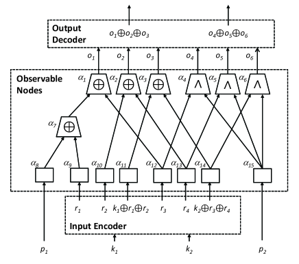
Figure 1: Example of a 2-leakage-resilient circuit

We associate a unique label (ranged over by $\alpha$) to every gate of the circuit. We call the nodes of $P$, ${\it nodes}({P})$, to be the set of labels in $P$ excluding the gates internal to the input encoder and the output decoder part of $P$ (but including the outputs of the input encoder and the inputs to the output decoder). Intuitively, ${\it nodes}({P})$ are the nodes that can be observed by the adversary. For example, in Fig. 1, the observable nodes are the ones in the region Observable Nodes labeled $\alpha_{1},\dots,\alpha_{15}$.

Let $\nu$ be a mapping from the inputs of $P$ to $\{{0,1}\}$. Let $\boldsymbol{\alpha}=\alpha_{1},\dots,\alpha_{n}$ be a vector of nodes in ${\it nodes}({P})$. We define the evaluation, ${\nu}_{P}({\boldsymbol{\alpha}})$, to be the vector $b_{1},\dots,b_{n}\in\{{0,1}\}^{n}$, such that each $b_{i}$ is the valuation of the node $\alpha_{i}$ when evaluating $P$ under $\nu$. For example, let $P^{\prime}$ be the circuit from Fig. 1. Let $\nu$ map $p_{1},r_{1},k_{2}$ to $0$, and the others to $1$. Then, ${\nu}_{P^{\prime}}({\alpha_{11},\alpha_{1}})=0,1$.

Let us write $\nu[\boldsymbol{v}\mapsto\boldsymbol{b}]$ for the store $\nu$ except that each $v_{i}$ is mapped to $b_{i}$ (for $i\in\{{1,\dots m}\}$) where $\boldsymbol{v}=v_{1},\dots,v_{m}$ and $\boldsymbol{b}=b_{1},\dots,b_{m}$. Let $P$ be a circuit with secret inputs $\boldsymbol{k}$, public inputs $\boldsymbol{p}$, and random inputs $\boldsymbol{r}$. For $\boldsymbol{b_{p}}\in\{{0,1}\}^{|p|}$, $\boldsymbol{b_{k}}\in\{{0,1}\}^{|k|}$, $\boldsymbol{\alpha}\in{\it nodes}({P})^{*}$, and $\boldsymbol{b_{\alpha}}\in\{{0,1}\}^{|\boldsymbol{\alpha}|}$, let $\#_{P}({\boldsymbol{b_{p}}},{\boldsymbol{b_{k}}},{\boldsymbol{\alpha}},{\boldsymbol{b_{\alpha}}})=|\{{\boldsymbol{b}\in\{{0,1}\}^{|\boldsymbol{r}|}\mid{\nu[\boldsymbol{r}\mapsto\boldsymbol{b}]}_{P}({\boldsymbol{\alpha}})=\boldsymbol{b_{\alpha}}}\}|$ where $\nu=\{{\boldsymbol{p}\mapsto\boldsymbol{b_{p}},\boldsymbol{k}\mapsto\boldsymbol{b_{k}}}\}$. We define $\mu_{P}({\boldsymbol{b_{p}}},{\boldsymbol{b_{k}}},{\boldsymbol{\alpha}})$ to be the finite map from each $\boldsymbol{b_{\alpha}}\in\{{0,1}\}^{|\boldsymbol{\alpha}|}$ to $\#_{P}({\boldsymbol{b_{p}}},{\boldsymbol{b_{k}}},{\boldsymbol{\alpha}},{\boldsymbol{b_{\alpha}}})$. We remark that $\mu_{P}({\boldsymbol{b_{p}}},{\boldsymbol{b_{k}}},{\boldsymbol{\alpha}})$, when normalized by the scaling factor $2^{-|\boldsymbol{r}|}$, is the joint distribution of the values of the nodes $\boldsymbol{\alpha}$ under the public inputs $\boldsymbol{b_{p}}$ and the secret inputs $\boldsymbol{b_{k}}$.

Roughly, the $n$-threshold-probing model of leakage resilience says that, for any selection of $n$ nodes, the joint distribution of the nodes’ values is independent of the secret. Formally, the leakage-resilience model is defined as follows.

Definition 1 (Leakage Resilience)

Let $P$ be an ${n}$$+$$1$-split circuit with secret inputs $\boldsymbol{k}$, public inputs $\boldsymbol{p}$, and random inputs $\boldsymbol{r}$. Then, $P$ is said to be leakage-resilient under the $n$-threshold-probing model (or, simply $n$-leakage-resilient) if for any $\boldsymbol{b_{p}}\in\{{0,1}\}^{|\boldsymbol{p}|}$, $\boldsymbol{b_{k}}\in\{{0,1}\}^{|\boldsymbol{k}|}$, $\boldsymbol{b_{k}}^{\prime}\in\{{0,1}\}^{|\boldsymbol{k}|}$, and $\boldsymbol{\alpha}\in{\it nodes}({P})^{n}$, $\mu_{P}({\boldsymbol{b_{p}}},{\boldsymbol{b_{k}}},{\boldsymbol{\alpha}})=\mu_{P}({\boldsymbol{b_{p}}},{\boldsymbol{b_{k}}^{\prime}},{\boldsymbol{\alpha}})$.

We remark that, above, $\boldsymbol{r}$ includes all randoms introduced by the input encoder as well as any additional ones that are not from the input encoder, if any. For instance, in the case of the circuit from Fig. 1, the randoms are $r_{1},r_{2},r_{3},r_{4}$ and they are all from the input encoder.

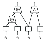
Figure 2: A circuit computing $(p_{1}\oplus k_{1}\oplus k_{2},k_{2}\wedge p_{2})$

Informally, the $n$-threshold-probing model of leakage resilience says that the attacker learns nothing about the secret by executing the circuit and observing the values of up to $n$ many internal gates and wires, excluding those that are internal to the input encoder and the output decoder.

We say that a circuit is random-free if it has no randoms. Let $P$ be a random-free circuit with public inputs $\boldsymbol{p}$ and secret inputs $\boldsymbol{k}$, and $P^{\prime}$ be a circuit with public inputs $\boldsymbol{p}$, secret inputs $\boldsymbol{k}$, and randoms $\boldsymbol{r}$. We say that $P^{\prime}$ is IO-equivalent to $P$ if for any $\boldsymbol{b_{k}}\in\{{0,1}\}^{|\boldsymbol{k}|}$, $\boldsymbol{b_{p}}\in\{{0,1}\}^{|\boldsymbol{p}|}$, and $\boldsymbol{b_{r}}\in\{{0,1}\}^{|\boldsymbol{r}|}$, the output of $P$ when evaluated under $\nu=\{{\boldsymbol{p}\mapsto\boldsymbol{b_{p}},\boldsymbol{k}\mapsto\boldsymbol{b_{k}}}\}$ is equivalent to that of $P^{\prime}$ when evaluated under $\nu[\boldsymbol{r}\mapsto\boldsymbol{b_{r}}]$. We formalize the synthesis problem.

Definition 2 (Synthesis Problem)

Given $n>0$ and a random-free circuit $P$ as input, the synthesis problem is the problem of building a circuit $P^{\prime}$ such that 1.) $P^{\prime}$ is IO-equivalent to $P$, and 2.) $P^{\prime}$ is $n$-leakage-resilient.

An important result by Ishai et al. [15] is that any random-free circuit can be converted to an IO-equivalent leakage-resilient form.

Theorem 2.1 ([15])

For any random-free circuit $P$, there exists an $n$-leakage-resilient circuit that is IO-equivalent to $P$.

While the result is of theoretical importance, the construction is more of a proof-of-concept in which every gate is transformed uniformly, and the obtained circuits can be quite unoptimized (e.g., injecting excess randoms to mask computations that do not depend on secrets). The subsequent research has proposed to construct more optimized leakage-resilient circuits manually [21, 5], or by automatic synthesis [8]. The latter is the direction of the present paper.

Example 1

Consider the random-free circuit $P$ shown in Fig. 2 which outputs $(p_{1}\oplus k_{1}\oplus k_{2},k_{2}\wedge p_{2})$. Let $P^{\prime}$ be the circuit from Fig. 1. It is easy to see that $P^{\prime}$ is IO-equivalent to $P$. Also, it can be shown that $P^{\prime}$ is $2$-leakage resilient. Therefore, $P^{\prime}$ is a $2$-leakage-resilient version of $P$.

Remark 1

The use of the input encoder and the output decoder is unavoidable. It is easy to see that the input encoder is needed. Indeed, without it, one cannot even defend against an one-node-observing attacker as she may directly observe the secret. To see that the output decoder is also required, consider an one-output circuit without the output decoder and let $n$ be the fan-in of the last gate before the output. Then, assuming that the output depends on the secret, the circuit cannot defend itself against an $n$-nodes-observing attacker as she may observe the inputs to the last gate.

Remark 2

In contrast to the previous works [5, 3] that implicitly assume that each secret is encoded (i.e., split in ${n}$$+$$1$ shares) by only one input encoder, we allow a secret to be encoded by multiple input encoders. The relaxation is important in our setting because, as remarked before, the compositionality results require disjointness of the randoms in the composed components.

Split and Non-Split Inputs / Outputs. We introduce terminologies that are convenient when describing the compositionality results in Section 3. We use the term split inputs to refer to the ${n}$$+$$1$ tuples of wires to which the ${n}$$+$$1$-split (secret) inputs produced by the input encoder (i.e., the pair of triples $r_{1},r_{2},k_{1}\oplus r_{1}\oplus r_{2}$ and $r_{3},r_{4},k_{2}\oplus r_{3}\oplus r_{4}$ in the example of Fig. 1) are passed, and use the term non-split inputs to refer to the wires to which the original inputs before the split (i.e., $k_{1}$ and $k_{2}$ in Fig. 1) are passed. We define split outputs and non-split outputs analogously. Roughly, the split inputs and outputs are the inputs and outputs of the attacker-observable part of the circuit (i.e., the region Observable Nodes in Fig. 1), whereas the non-split inputs and outputs are those of the whole circuit with the input encoder and the output decoder.

3 Compositionality of Leakage Resilience

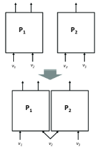
Figure 3: Parallel composition of $P_{1}$ and $P_{2}$.

This section shows the compositionality property of the $n$-threshold-probing model of leakage resilience. We state and prove two main results (for space the proofs are deferred to Appendix).

The first result concerns parallel compositions. It shows that given two $n$-leakage-resilient circuits $P_{1}$ and $P_{2}$ that possibly share inputs, the composed circuit that runs $P_{1}$ and $P_{2}$ in parallel is also $n$-leakage resilient, assuming that the randoms in the two components are disjoint. Fig. 3 shows the diagram depicting the composition. The second result concerns sequential compositions, and it is significantly harder to prove than the first one. The sequential composition takes an $n$-leakage-resilient circuit $P_{2}$ having $y$ many (non-split) inputs, and $n$-leakage-resilient circuits $P_{11},\dots,P_{1y}$ each having one (non-split) output. The composition is done by connecting each split output of the output-decoder-free part of $P_{1i}$ to the $i$th split input of the input-encoder-free part of $P_{2}$. Clearly, the composed circuit is IO-equivalent to the one formed by connecting each non-split output of $P_{1i}$ to the $i$th non-split input of $P_{2}$. The sequential compositionality result states that the composed circuit is also $n$-leakage resilient, under the assumption that the randoms in the composed components are disjoint. Fig. 4 shows the diagram of the composition. We state and prove the parallel compositionality result formally in Section 3.1, and the sequential compositionality result in Section 3.2.

We remark that, in the sequential composition, if a (non-split) secret input, say $k$, is shared by some $P_{1i}$ and $P_{1j}$ for $i\neq j$, then the disjoint randomness condition requires $k$ to be encoded by two independent input encoders. This is in contrast to the previous works [5, 3] that only use one input encoder per a secret input. On the other hand, such works require additional randoms at the site of the composition, whereas no additional randoms are needed at the composition site in our case as it directly connects the split outputs of $P_{1i}$’s to the split inputs of $P_{2}$.

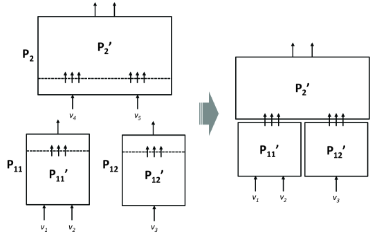
Figure 4: Sequential composition of $P_{11}$, $P_{12}$, and $P_{2}$. Here, ${P_{11}}^{\prime}$ (resp. ${P_{12}}^{\prime}$) is the output-decoder-free part of $P_{11}$ (resp. $P_{12}$), and ${P_{2}}^{\prime}$ is the input-encoder-free part of $P_{2}$. The composition connects the split outputs of ${P_{11}}^{\prime}$ and ${P_{12}}^{\prime}$ to the split inputs of ${P_{2}}^{\prime}$.

3.1 Parallel Composition

This subsection proves the parallel compositionality result. Let us write ${P_{1}}||{P_{2}}$ for the parallel composition of $P_{1}$ and $P_{2}$. We state and prove the result.

Theorem 3.1

Let $P_{1}$ and $P_{2}$ be $n$-leakage-resilient circuits having disjoint randoms. Then, ${P_{1}}||{P_{2}}$ is also $n$-leakage-resilient.

Remark 3

While Theorem 3.1 only states that ${P_{1}}||{P_{2}}$ can withstand an attack that observes up to $n$ nodes total from the composed circuit, a stronger property can actually be derived from the proof of the theorem. That is, the proof shows that ${P_{1}}||{P_{2}}$ can withstand an attack that observes up to $n$ nodes from the $P_{1}$ part and up to $n$ nodes from the $P_{2}$ part. (However, it is not secure against an attack that picks more than $n$ nodes in an arbitrary way: for example, picking $n+1$ nodes from one side.)

3.2 Sequential Composition

This subsection proves the sequential compositionality result. As remarked above, the result is significantly harder to prove than the parallel compositionality result. Let us write $({P_{11},\dots,P_{1y}})\mathbin{\rhd}{P_{2}}$ for the sequential composition of $P_{11},\dots,P_{1y}$ with a $y$-input circuit $P_{2}$. We state and prove the sequential compositionality result.

Theorem 3.2

Let $P_{11},\dots,P_{1y}$ be $n$-leakage-resilient circuits, and $P_{2}$ be an $y$-input $n$-leakage-resilient circuit, having disjoint randoms. Then, $({P_{11},\dots,P_{1y}})\mathbin{\rhd}{P_{2}}$ is $n$-leakage-resilient.

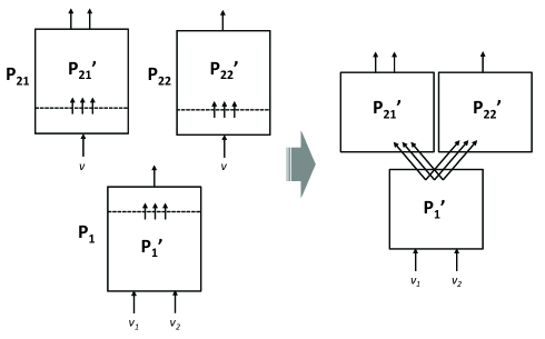
Figure 5: Output-sharing sequential composition of $P_{1}$, $P_{21}$, and $P_{22}$. Here, ${P_{1}}^{\prime}$ is the output-decoder-free part of $P_{1}$, and ${P_{21}}^{\prime}$ (resp. ${P_{22}}^{\prime}$) is the input-encoder-free part of $P_{21}$ (resp. $P_{22}$). The composition connects the split output of ${P_{1}}^{\prime}$ to the split inputs of ${P_{21}}^{\prime}$ and ${P_{22}}^{\prime}$.

Example 2

As remarked in Section 3, the parallel compositionality result enjoys an additional property that the circuit is secure even under an attack that observes more than $n$ nodes in the composition as long as the observation in each component is at most $n$. We show that the property does not hold in the case of sequential composition. Indeed, it can be shown that just allowing $n+1$ observations breaks the security even if the number of observations made within each component is at most $n$.

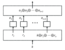
Figure 6: An $n$-leakage resilient identity circuit.

To see this, consider the ${n}$$+$$1$-split circuit shown in Fig. 6. The circuit implements the identity function, and it is easy to see that the circuit is $n$-leakage resilient. Let $P_{1}$ and $P_{2}$ be copies of the circuit, and consider the composition $({P_{1}})\mathbin{\rhd}{P_{2}}$. Then, the composed circuit is not secure against an attack that observes $m$ nodes of $P_{1}$ for some $1\leq m\leq n$, and observes $n+1-m$ nodes of $P_{2}$ such that the nodes picked on the $P_{2}$ side are the nodes connected to the nodes that are not picked on the $P_{1}$ side.

Remark 4

By a reasoning similar to the one used in the proof of Theorem 3.2, we can show the correctness of a more parsimonious version of parallel composition theorem (Theorem 3.1) where given $P_{1}$ and $P_{2}$ that shares a secret, instead of ${P_{1}}||{P_{2}}$ duplicating split shares of the secret as in Fig. 3, we make one split share tuple to be used in the both sides of the composition. Combining this improved parallel composition with the sequential compositionality result, we obtain compositionality for the case where an output of a circuit is shared by more than one circuit in a sequential composition.

Fig. 5 depicts such an output-sharing sequential composition. Here, $P_{1}$, $P_{21}$, and $P_{22}$ are $n$-leakage-resilient circuits, and we wish to compose them by connecting the output of $P_{1}$ to the input of $P_{21}$ and the input of $P_{22}$. By the parallel compositionality result, the parallel composition of $P_{21}$ and $P_{22}$ that shares the same input ($v$) is $n$-leakage-resilient. Then, it follows that, sequentially composing that parallelly composed circuit with $P_{1}$, as depicted in the figure, is also $n$-leakage-resilient thanks to the sequential compositionality result.

4 Compositional Synthesis Algorithm

The compositionality property gives a way for a compositional approach to synthesizing leakage-resilient circuits. Algorithm 1 shows the overview of the synthesis algorithm. Given a random-free circuit as an input, the algorithm synthesizes an IO-equivalent $n$-leakage-resilient circuit. It first invokes the Decomp operation to choose a suitable decomposition of the given circuit into some number of sub-circuits. Then, it invokes MonoSynth on each sub-circuit $P_{i}$ to synthesize an $n$-leakage resilient circuit ${P_{i}}^{\prime}$ that is IO-equivalent to $P_{i}$. Finally, it returns the composition of the obtained circuits as the synthesized $n$-leakage resilient version of the original.

Algorithm 1 The Compositional Synthesis Algorithm

1:Random-free Circuit $P$

2:IO-equivalent $n$-leakage-resilient circuit

3:$P_{1},\dots,P_{m}$ := $\textsc{Decomp}(P)$

4:for each $P_{i}\in\{P_{1},\dots,P_{m}\}$ do

5:     ${P_{i}}^{\prime}$ := $\textsc{MonoSynth}(P_{i})$

6:end for

7:return $\textsc{Comp}({P_{1}}^{\prime},\dots,{P_{m}}^{\prime})$

Comp is the composition operation, and it composes the given $n$-leakage-resilient circuits in the manner described in Section 3. MonoSynth is a constraint-based “monolithic” synthesis algorithm that synthesizes an $n$-leakage-resilient circuit that is IO-equivalent to the given circuit without further decomposition. We describe MonoSynth in Section 4.1, and describe the decomposition operation Decomp in Section 4.2.

The algorithm optimizes the synthesized circuits in the following ways. First, as described in Section 4.1, the monolithic synthesis looks for tree-shaped circuits of the shortest tree height. Secondly, as described in Section 4.2, the decomposition and composition is done in a way to avoid unnecessarily making the non-secret-dependent parts leakage resilient, and also to re-use the synthesis results for shared sub-circuits whenever allowed by the compositionality properties.

Remark 5

The compositional algorithm composes the $n$-leakage-resilient versions of the sub-circuits. Note that the compositionality property states that the result will be $n$-leakage-resilient after the composition, regardless of how the sub-circuits are synthesized as long as they are also $n$-leakage-resilient and have disjoint randoms. Thus, in principle, any method to synthesize the $n$-leakage-resilient versions of the sub-circuits may be used in place of MonoSynth. For instance, a possible alternative is to use a database of $n$-leakage-resilient versions of commonly-used circuits (e.g., obtained via the construction of [15, 5]).

4.1 Constraint-Based Monolithic Synthesis

The monolithic synthesis algorithm is based on and extends the constraint-based approach proposed by Eldib and Wang [8]. The algorithm synthesizes an $n$-leakage-resilient circuit that is IO-equivalent to the given circuit. The algorithm requires the given circuit to have only one output. Therefore, the overall algorithm to decomposes the whole circuit into such sub-circuits before passing them to MonoSynth.

We formalize the algorithm as quantified first-order logic constraint solving. Let $P$ be the random-free circuit given as the input. We prepare a quantifier-free formula $\Phi_{P}(\boldsymbol{\alpha},\boldsymbol{p},\boldsymbol{k},o)$ on the free variables $\boldsymbol{\alpha}$, $\boldsymbol{p}$, $\boldsymbol{k}$, $o$ that encodes the input-output behavior of $P$. Formally, $\exists\boldsymbol{\alpha}.\Phi_{P}(\boldsymbol{\alpha},\boldsymbol{p},\boldsymbol{k},o)$ is true iff $P$ outputs $o$ given public inputs $\boldsymbol{p}$ and secret inputs $\boldsymbol{k}$. The variables $\boldsymbol{\alpha}$ are used for encoding the shared sub-circuits within $P$ (i.e., gates of fan-out $>1$). For example, for $P$ that outputs $k\wedge p$, $\Phi_{P}(p,k,o)\equiv o=k\wedge p$.

$\begin{array}[]{l}o=\alpha_{1}\oplus\alpha_{4}\ \wedge\\ \bigwedge_{i\in\{{1,4}\}}((C_{i}=\texttt{XOR}\Rightarrow\alpha_{i}=\alpha_{i+1}\oplus\alpha_{i+2})\ \wedge\\ \hskip 40.00006pt(C_{i}=\texttt{AND}\Rightarrow\alpha_{i}=\alpha_{i+1}\wedge\alpha_{i+2})\ \wedge\\ \hskip 40.00006pt(C_{i}=\texttt{OR}\Rightarrow\alpha_{i}=\alpha_{i+1}\vee\alpha_{i+2}))\ \wedge\\ \bigwedge_{i\in\{{2,3,5,6}\}}((C_{i}=\texttt{F}\Rightarrow\alpha_{i}=0)\wedge(C_{i}=\texttt{T}\Rightarrow\alpha_{i}=1)\ \wedge\\ \hskip 52.00005pt(C_{i}=\texttt{P}\Rightarrow\alpha_{i}=p)\wedge(C_{i}=\texttt{K1}\Rightarrow\alpha_{i}=r)\ \wedge\\ \hskip 52.00005pt(C_{i}=\texttt{K2}\Rightarrow\alpha_{i}=k\oplus r))\end{array}$

(a)

(b)

Figure 7: (a) Skeleton circuit. (b) $\Phi_{\textit{Sk}_{2}}$ for the skeleton circuit.

Adopting the approach of [8], our monolithic algorithm works by preparing skeleton circuits of increasing size, and searching for an instance of the skeleton that is $n$-leakage-resilient and IO-equivalent to $P$. By starting from a small skeleton, the algorithm biases toward finding an optimized leakage resilient circuit. Formally, a skeleton circuit $\textit{Sk}_{\ell}$ is a tree-shaped circuit (i.e., circuit with all non-input gates having fan-out of $1$) of height $\ell$ whose gates have undetermined functionality except for the parts that implement the input encoder and the output decoder. For example, Fig. 7 (a) shows the ${1}$$+$$1$-split skeleton circuit of height $2$ with one secret input.

We prepare a quantifier-free skeleton formula $\Phi_{\textit{Sk}_{\ell}}$ that expresses the skeleton circuit. Formally, $\Phi_{\textit{Sk}_{\ell}}(\boldsymbol{C},\boldsymbol{\alpha},\boldsymbol{p},\boldsymbol{k},\boldsymbol{r},o)$ is true iff $P^{\prime}$ outputs $o$ with the valuations of ${\it nodes}({P^{\prime}})$ having the values $\boldsymbol{\alpha}$ given public inputs $\boldsymbol{p}$, secret inputs $\boldsymbol{k}$, and random inputs $\boldsymbol{r}$ where $P^{\prime}$ is $\textit{Sk}_{\ell}$ with its nodes’ functionality determined by $\boldsymbol{C}$. We call $\boldsymbol{C}$ the control variables, and write $\textit{Sk}_{\ell}(\boldsymbol{C})$ for the instance of $\textit{Sk}_{\ell}$ determined by $\boldsymbol{C}$. For example, Fig. 7 (b) shows $\Phi_{\textit{Sk}_{\ell}}$ for the skeleton circuit from Fig. 7 (a), when there is one public input and no randoms besides the one from the input encoder.

The synthesis is now reduced to the problem of finding an assignment to $\boldsymbol{C}$ that satisfies the constraint $\Phi_{\textsc{io}}(\boldsymbol{C})\wedge\Phi_{\textsc{lr}}(\boldsymbol{C})$ where $\Phi_{\textsc{io}}(\boldsymbol{C})$ expresses that $\textit{Sk}_{\ell}(\boldsymbol{C})$ is IO-equivalent to $P$, and $\Phi_{\textsc{lr}}(\boldsymbol{C})$ expresses that $\textit{Sk}_{\ell}(\boldsymbol{C})$ is $n$-leakage-resilient. As we shall show next, the constraints faithfully encode IO-equivalence and leakage-resilience according to the definitions from Section 2.

$\Phi_{\textsc{io}}(\boldsymbol{C})$ is the formula below.

$$\begin{array}[]{l}\forall\boldsymbol{\alpha},\boldsymbol{\alpha^{\prime}},\boldsymbol{p},\boldsymbol{k},\boldsymbol{r},o,o^{\prime}.\ \Phi_{P}(\boldsymbol{\alpha},\boldsymbol{p},\boldsymbol{k},o)\wedge\Phi_{\textit{Sk}_{\ell}}(\boldsymbol{C},\boldsymbol{\alpha^{\prime}},\boldsymbol{p},\boldsymbol{k},\boldsymbol{r},o^{\prime})\Rightarrow o=o^{\prime}\end{array}$$

It is easy to see that $\Phi_{\textsc{io}}$ correctly expresses IO equivalence.

The definition of $\Phi_{\textsc{lr}}$ is more involved, and we begin by introducing a useful shorthand notation. Let $m$ be the number of (observable) nodes in $\textit{Sk}_{\ell}$. Without loss of generality, we assume that $m\geq n$. Let $\boldsymbol{\sigma}\in\{{1,\dots,m}\}^{*}$ be a sequence such that $|\boldsymbol{\sigma}|\leq n$, and $\boldsymbol{\alpha}=\alpha_{1},\dots,\alpha_{m}$ be a length $m$ sequence of variables. We write ${\boldsymbol{\alpha}}\langle{\boldsymbol{\sigma}}\rangle$ for the sequence of variables $\beta_{1},\dots\beta_{|\boldsymbol{\sigma}|}$ such that $\beta_{i}=\alpha_{\sigma_{i}}$ for each $i\in\{{1,\dots,|\boldsymbol{\sigma}|}\}$. Intuitively, $\boldsymbol{\sigma}$ represents a selection of nodes observed by the adversary. For example, let $\boldsymbol{\alpha}=\alpha_{1},\alpha_{2},\alpha_{3}$ and $\boldsymbol{\sigma}=1,3$, then ${\boldsymbol{\alpha}}\langle{\boldsymbol{\sigma}}\rangle=\alpha_{1},\alpha_{3}$.

Let $\mathcal{R}=\{{0,1}\}^{|\boldsymbol{r}|}$. Then, $\Phi_{\textsc{lr}}(\boldsymbol{C})$ is the formula below.

$$\begin{array}[]{l}\forall\boldsymbol{\sigma}.\forall\boldsymbol{\beta},\boldsymbol{\alpha}^{\prime},\boldsymbol{p},\boldsymbol{k},\boldsymbol{k}^{\prime},\boldsymbol{o}.\\ \hskip 15.00002pt\bigwedge_{\boldsymbol{b}\in\mathcal{R}}\phi[\boldsymbol{\alpha_{b}}/\boldsymbol{\alpha}][o_{\boldsymbol{b}}/o]\wedge\phi[\boldsymbol{\alpha^{\prime}_{b}}/\boldsymbol{\alpha}][o^{\prime}_{\boldsymbol{b}}/o][\boldsymbol{k^{\prime}}/\boldsymbol{k}]\\ \hskip 30.00005pt\Rightarrow\ \sum_{\boldsymbol{b}\in\mathcal{R}}({\boldsymbol{\alpha_{b}}}\langle{\boldsymbol{\sigma}}\rangle=\boldsymbol{\beta})=\sum_{\boldsymbol{b}\in\mathcal{R}}({\boldsymbol{\alpha_{b}}^{\prime}}\langle{\boldsymbol{\sigma}}\rangle=\boldsymbol{\beta})\end{array}$$

where $\boldsymbol{\alpha}^{\prime}$ is a sequence comprising distinct variables $\boldsymbol{\alpha_{b}}$ and $\boldsymbol{\alpha^{\prime}_{b}}$ such that $|\boldsymbol{\alpha_{b}}|=|\boldsymbol{\alpha^{\prime}_{b}}|=m$ for each $\boldsymbol{b}\in\mathcal{R}$, $\boldsymbol{o}$ is a sequence comprising distinct variables $o_{\boldsymbol{b}}$ and $o^{\prime}_{\boldsymbol{b}}$ for each $\boldsymbol{b}\in\mathcal{R}$, and $\phi$ is the formula $\Phi_{\textit{Sk}_{\ell}}(\boldsymbol{C},\boldsymbol{\alpha},\boldsymbol{p},\boldsymbol{k},\boldsymbol{b},o)$. While $\Phi_{\textsc{lr}}(\boldsymbol{C})$ is not strictly a first-order logic formula, it can be converted to the form by expanding the finitely many possible choices of $\boldsymbol{\sigma}$.

Algorithm 2 MonoSynth

1:Random-free Circuit $P$

2:IO-equivalent $n$-leakage resilient circuit

3:$\ell$ := INIT_HEIGHT

4:loop

5:     tset := $\emptyset$; $\gamma$ := $n$

6:     loop

7:         match FindCand(tset,$\gamma$) with

8:             nosol $\rightarrow$ $\ell$++; break

9:            $\mid$ $\textsf{sol}(\boldsymbol{b_{C}})$ $\rightarrow$ match CheckCand($\boldsymbol{b_{C}}$) with

10:                                 success $\rightarrow$ return $\textit{Sk}_{\ell}(\boldsymbol{b_{C}})$

11:                               $\mid$ $\textsf{cex}(\textit{tset}^{\prime},\gamma^{\prime})$ $\rightarrow$ tset := $\textit{tset}\cup\textit{tset}^{\prime}$; $\gamma$ := $\textit{max}(\gamma,\gamma^{\prime})$

12:     end loop

13:end loop

Because the domains of the quantified variables in $\Phi_{\textsc{io}}$ and $\Phi_{\textsc{lr}}$ are finite, one approach to solving the constraint may be first eliminating the quantifiers eagerly and then solving for $\boldsymbol{C}$ that satisfies the resulting constraint. However, the approach is clearly impractical due to the extreme size of the resulting constraint. Instead, adopting the idea from [8], we solve the constraint by lazily instantiating the quantifiers. The main idea is to divide the constraint solving process in two phases: the candidate finding phase that infers a candidate solution for $\boldsymbol{C}$, and the candidate checking phase that checks whether the candidate is actually a solution. We run the phases iteratively in a CEGAR style until convergence. Algorithm 2 shows the overview of the process. We describe the details of the algorithm below.

Candidate Checking. The candidate checking phase is straightforward. Note that, after expanding the choices of $\boldsymbol{\sigma}$ in $\Phi_{\textsc{lr}}$, $\Phi_{\textsc{io}}(\boldsymbol{C})\wedge\Phi_{\textsc{lr}}(\boldsymbol{C})$ only has outer-most $\forall$ quantifiers. Therefore, given a concrete assignment to $\boldsymbol{C}$, $\boldsymbol{b_{C}}$, CheckCand directly solves the the constraint by using an SMT solver. (However, naively expanding $\boldsymbol{\sigma}$ can be costly when $n>1$, and we show a modification that alleviates the cost in the later part of the subsection.)

Candidate Finding. We describe the candidate finding process FindCand. To find a likely candidate, we adopt the idea from [8] and prepare a test set that is updated via the CEGAR iterations. In [8], a test set, tset, is a pair of sets $\textit{tset}_{p}$ and $\textit{tset}_{k}$ where $\textit{tset}_{p}$ (resp. $\textit{tset}_{k}$) contains finitely many concrete valuations of $\boldsymbol{p}$ (resp. $\boldsymbol{k}$). Having such a test set, we can rewrite the constraint so that the public inputs and secret inputs are restricted to those from the test set. That is, $\Phi_{\textsc{io}}(\boldsymbol{C})$ is rewritten to be the formula below.

$$\begin{array}[]{l}\bigwedge_{(\boldsymbol{b_{p}},\boldsymbol{b_{k}})\in\textit{tset}_{p}\times\textit{tset}_{k}}\\ \hskip 5.0pt\Phi_{P}(\boldsymbol{\alpha_{\boldsymbol{b_{p}}\boldsymbol{b_{k}}{}}},\boldsymbol{b_{p}},\boldsymbol{b_{k}},o_{\boldsymbol{b_{p}}\boldsymbol{b_{k}}{}})\wedge\Phi_{\textit{Sk}_{\ell}}(\boldsymbol{C},\boldsymbol{\alpha^{\prime}_{\boldsymbol{b_{p}}\boldsymbol{b_{k}}{}}},\boldsymbol{b_{p}},\boldsymbol{b_{k}},\boldsymbol{r_{\boldsymbol{b_{p}}\boldsymbol{b_{k}}{}}},o^{\prime}_{\boldsymbol{b_{p}}\boldsymbol{b_{k}}{}})\wedge o_{\boldsymbol{b_{p}}\boldsymbol{b_{k}}{}}=o^{\prime}_{\boldsymbol{b_{p}}\boldsymbol{b_{k}}{}}\end{array}$$

And, $\Phi_{\textsc{lr}}(\boldsymbol{C})$ becomes the formula below.

$$\begin{array}[]{l}\forall\boldsymbol{\sigma}.\forall\boldsymbol{\beta}.\bigwedge_{(\boldsymbol{b_{p}},\boldsymbol{b_{k}},\boldsymbol{b_{k}}^{\prime})\in\textit{tset}_{p}\times\textit{tset}_{k}\times\textit{tset}_{k}}\bigwedge_{\boldsymbol{b}\in\mathcal{R}}\\ \hskip 10.00002pt\phi[\boldsymbol{\alpha}_{\boldsymbol{b_{p}}\boldsymbol{b_{k}}{}\boldsymbol{b}}/\boldsymbol{\alpha}][o_{\boldsymbol{b_{p}}\boldsymbol{b_{k}}{}\boldsymbol{b}}/o][\boldsymbol{b_{k}}/\boldsymbol{k}]\wedge\phi[\boldsymbol{\alpha}^{\prime}_{\boldsymbol{b_{p}}\boldsymbol{b_{k}^{\prime}}{}\boldsymbol{b}}/\boldsymbol{\alpha}][o^{\prime}_{\boldsymbol{b_{p}}\boldsymbol{b_{k}^{\prime}}{}\boldsymbol{b}}/o][\boldsymbol{b_{k}^{\prime}}/\boldsymbol{k}]\\ \hskip 10.00002pt\wedge\ \sum_{\boldsymbol{b}\in\mathcal{R}}({\boldsymbol{\alpha_{\boldsymbol{b_{p}}\boldsymbol{b_{k}}{}\boldsymbol{b}}}}\langle{\boldsymbol{\sigma}}\rangle=\boldsymbol{\beta})=\sum_{\boldsymbol{b}\in\mathcal{R}}({\boldsymbol{\alpha^{\prime}_{\boldsymbol{b_{p}}\boldsymbol{b_{k}^{\prime}}{}\boldsymbol{b}}}}\langle{\boldsymbol{\sigma}}\rangle=\boldsymbol{\beta})\end{array}$$

where $\phi$ is the formula $\Phi_{\textit{Sk}_{\ell}}(\boldsymbol{C},\boldsymbol{\alpha},\boldsymbol{b_{p}},\boldsymbol{k},\boldsymbol{b},o)$. We remark that, because fixing the inputs to concrete values also fixes the valuations of some other variables (e.g., fixing $\boldsymbol{p}$ and $\boldsymbol{k}$ also fixes $\boldsymbol{\alpha}$ and $o$ in $\Phi_{P}(\boldsymbol{\alpha},\boldsymbol{p},\boldsymbol{k},o)$), the constraint structure is modified to remove the quantifications on such variables.

At this point, the approach of [8] can be formalized as the following process: it eagerly instantiates the possible choices of $\boldsymbol{\sigma}$ and $\boldsymbol{\beta}$ to reduce the constraint to a quantifier-free form, and looks for a satisfying assignment to the resulting constraint. This is a sensible approach when $n$ is $1$ because, in that case, the number of possible choices of $\boldsymbol{\sigma}$ is linear in the size of the skeleton (i.e., is $m$) and the possible valuations of $\boldsymbol{\beta}$ are simply $\{{0,1}\}$. Unfortunately, the number of possible choices of $\boldsymbol{\sigma}$ grows exponentially in $n$, and so does that of the possible valuations of $\boldsymbol{\beta}$. We remark that this is expected because $\boldsymbol{\sigma}$ represents the adversary’s node selection choice, and $\boldsymbol{\beta}$ represents the valuation of the selected nodes. Indeed, in our experience with a prototype implementation, this method fails even on quite small sub-circuits when $n$ is even $2$.

Therefore, we make the following improvements to the base algorithm.

• We restrict the node selection to root-most $\gamma$ nodes where $\gamma$ starts at $n$ and is incremented via the CEGAR loop.

• We include node valuations in the test set.

• We use dependency analysis to reduce irrelevant node selections from the constraint in the candidate checking phase.

The rationale for prioritizing the root-most nodes in (1) is that, in a tree-shaped circuit, nodes closer to the root are more likely to be dependent on the secret and therefore are expected to be better targets for the adversary. The number of root-most nodes to select, $\gamma$, is incremented as needed by a counterexample analysis (cf. lines 7-9 of Algorithm 2). The test set generation for node valuations described in item (2) is done in much the same way as that for public inputs and secret inputs. We describe the test set generation process in more detail in Test Set Generation. With the modifications (1) and (2), the leakage-resilience constraint to be solved in the candidate finding phase is now the following formula.

$$\begin{array}[]{l}\forall\boldsymbol{\sigma}:\gamma.\bigwedge_{(\boldsymbol{b_{p}},\boldsymbol{b_{k}},\boldsymbol{b_{k}}^{\prime},\boldsymbol{b_{\beta}})\in\textit{tset}_{p}\times\textit{tset}_{k}\times\textit{tset}_{k}\times\textit{tset}_{\beta}}\bigwedge_{\boldsymbol{b}\in\mathcal{R}}\\ \hskip 10.00002pt\phi[\boldsymbol{\alpha}_{\boldsymbol{b_{p}}\boldsymbol{b_{k}}{}\boldsymbol{b}}/\boldsymbol{\alpha}][o_{\boldsymbol{b_{p}}\boldsymbol{b_{k}}{}\boldsymbol{b}}/o][\boldsymbol{b_{k}}/\boldsymbol{k}]\wedge\phi[\boldsymbol{\alpha}^{\prime}_{\boldsymbol{b_{p}}\boldsymbol{b_{k}^{\prime}}{}\boldsymbol{b}}/\boldsymbol{\alpha}][o^{\prime}_{\boldsymbol{b_{p}}\boldsymbol{b_{k}^{\prime}}{}\boldsymbol{b}}/o][\boldsymbol{b_{k}^{\prime}}/\boldsymbol{k}]\\ \hskip 10.00002pt\wedge\ \sum_{\boldsymbol{b}\in\mathcal{R}}({\boldsymbol{\alpha_{\boldsymbol{b_{p}}\boldsymbol{b_{k}}{}\boldsymbol{b}}}}\langle{\boldsymbol{\sigma}}\rangle=\boldsymbol{b_{\beta}})=\sum_{\boldsymbol{b}\in\mathcal{R}}({\boldsymbol{\alpha^{\prime}_{\boldsymbol{b_{p}}\boldsymbol{b_{k}^{\prime}}{}\boldsymbol{b}}}}\langle{\boldsymbol{\sigma}}\rangle=\boldsymbol{b_{\beta}})\end{array}$$

where $\boldsymbol{\sigma}:\gamma$ restricts $\boldsymbol{\sigma}$ to the root most $\gamma$ indexes, $\textit{tset}_{\beta}$ is the set of test set elements for node valuations, and $\phi$ is the formula $\Phi_{\textit{Sk}_{\ell}}(\boldsymbol{C},\boldsymbol{\alpha},\boldsymbol{b_{p}},\boldsymbol{k},\boldsymbol{b},o)$.

Unlike (1) and (2), the modification (3) applies to the candidate checking phase. To see the benefit of this modification, note that, even in the candidate checking phase, checking the leakage-resilience condition $\Phi_{\textsc{lr}}(\boldsymbol{b_{C}})$ can be quite expensive because it involves expanding exponentially many possible choices of node selections. To mitigate the cost, we take advantage of the fact that the candidate circuit is fixed in the candidate checking phase, and do a simple dependency analysis on the candidate circuit to reduce irrelevant node-selection choices. We describe the modification in more detail. Let $P^{\prime}$ be the candidate circuit. For each node of $P^{\prime}$, we collect the reachable leafs from the node to obtain the over-approximate set of inputs on which the node may depend. For a node $\alpha$ of $P^{\prime}$, let $\textit{deps}({\alpha})$ be the obtained set of dependent inputs for $\alpha$. Then, any selection of nodes $\boldsymbol{\alpha}$ such that $\bigcup_{\alpha\in\{{\boldsymbol{\alpha}}\}}\textit{deps}({\alpha})$ does not contain all ${n}$$+$$1$-split shares of some secret is an irrelevant selection and can be removed from the constraint. (Here, we use the symbols $\alpha$ for node labels as in Section 2, and not as node-valuation variables in a constraint.)

Test Set Generation. Recall that our algorithm maintains three kinds of test sets, $\textit{tset}_{p}$ for public inputs, $\textit{tset}_{k}$ for secret inputs, and $\textit{tset}_{\beta}$ for node valuations. As shown in lines 7-9 of Algorithm 2, we obtain new test set elements from candidate check failures (here, by abuse of notation, we write $\textit{tset}\cup\textit{tset}^{\prime}$ for the component-wise union). We describe the process in more detail. In CheckCand, we convert the constraint $\Phi_{\textsc{io}}(\boldsymbol{b_{C}})\wedge\Phi_{\textsc{lr}}(\boldsymbol{b_{C}})$ to a quantifier free formula $\Phi$ by expanding the selection choices and removing the universal quantifiers. Then, we use an SMT solver to check the satisfiability of $\neg\Phi$ and return success if it is unsatisfiable. Otherwise, the SMT solver returns a satisfying assignment of $\neg\Phi$, and we return the values assigned to variables corresponding to public inputs, secret inputs and node valuations as the new elements for the respective test sets. The number of root-most nodes to select is also raised here by taking the maximum of the root-most nodes observed in the satisfying assignment, $\gamma^{\prime}$, with the current $\gamma$.

4.2 Choosing Decomposition

This subsection describes the decomposition procedure Decomp. Thanks to the generality of the compositionality results, in principle, we can decompose the given circuit into arbitrarily small sub-circuits (i.e., down to individual gates). However, choosing a too fine-grained decomposition may lead to a sub-optimal result.

To this end, we have implemented the following decomposition strategy. First, we run a dependency analysis, similar to the one used in the constraint-based monolithic synthesis (cf. Section 4.1). The analysis result is used to identify the parts of the given circuit that do not depend on any of the secrets. We factor out such public-only sub-circuits from the rest so that they will not be subject to the leakage-resilience transformation.

Next, we look for sub-circuits that are used at multiple locations (i.e., whose roots have fan-out $>1$), and prioritize them to be synthesized separately and composed at their use sites. Besides the saving in the synthesis effort, the approach can lead a smaller synthesis result when the shared sub-circuit is used in contexts that lead to different outputs (cf Remark 4). Finally, as a general strategy, we apply parallel composition at the root so that we synthesize separately for each output given a multi-output circuit. And, we set a bound on the maximum size of the circuits that will be synthesized monolithically, and decompose systematically based on the bound. As discussed in Section 5, in the prototype implementation, we use an “adaptive” version of the latter decomposition process by adjusting the bound on-the-fly and also opts for a pre-made circuit under certain conditions.

Example 3

Let us apply the compositional synthesis algorithm to the circuit from Fig. 2, for the case $n=2$. Note that the circuit has no non-trivial public-only sub-circuits or have non-inputs gates with fan-out greater than $1$.

First, we apply the parallel compositionality result so that the circuit is decomposed to two parts: the left tree that computes $p_{1}\oplus k_{1}\oplus k_{2}$ and the right tree that computes $k_{2}\oplus p_{2}$. The right tree cannot be decomposed further, and we apply MonoSynth to transform it to a leakage-resilient form. A possible synthesis result of this is the right sub-circuit shown in Fig. 1 (i.e., the sub-circuit whose observable part outputs the split output $o_{4},o_{5},o_{6}$).

For the left tree, if the monolithic-synthesis size bound is set to synthesize circuits of height $2$, we apply MonoSynth directly to the tree. Alternatively, with a lower bound set, we further decompose the left tree to a lower part that computes $p_{1}\oplus k_{1}$ and $p_{2}$ (identity function) and an upper part that computes $k\oplus p_{2}$ where the output of the lower part is to be connected to the “place-holder” input $k$. Following the either strategy, we may obtain the the left sub-circuit of Fig. 1 as a possible result. And, the final synthesis result after composing the left and right synthesis results is the whole circuit of Fig. 1.

5 Implementation and Experiments

name	$n=2$			$n=3$			$n=4$			name	$n=2$			$n=3$			$n=4$
	time	size	rds	time	size	rds	time	size	rds		time	size	rds	time	size	rds	time	size	rds
P1	16.2s	123	32	49.4s	138	48	52.7s	160	64	P10	T/O			M/O			M/O
P2	10.3s	64	16	1m13s	76	24	4m3s	88	32	P11	T/O			T/O			M/O
P3	M/O			M/O			M/O			P12	T/O			T/O			T/O
P4	M/O			M/O			M/O			P13	T/O			T/O			T/O
P5	M/O			M/O			M/O			P14	T/O			T/O			M/O
P6	M/O			M/O			M/O			P15	T/O			T/O			M/O
P7	M/O			M/O			M/O			P16	T/O			T/O			T/O
P8	M/O			M/O			M/O			P17	T/O			T/O			T/O
P9	T/O			T/O			T/O			P18	T/O			T/O			T/O

Table 1: Experiment Results: Monolithic Only.

name	$n=2$				$n=3$				$n=4$
	time	mtc	size	rds	time	mtc	size	rds	time	mtc	size	rds
P1	18.7s	2.7s	125	32	30.2s	4.5s	143	48	1m1s	33.3s	160	64
P2	11.8s	3.6s	65	16	1m7s	17.3s	74	24	2m56s	1m21s	88	32
P3	2.7s	0.8s	50	11	12.3s	6.9s	83	18	3m57s	1m4s	120	26
P4	3.9s	3.1s	42	9	4.5s	2.1s	69	15	1m48s	1m4s	100	22
P5	5.9s	2.1s	63	13	20.2s	6.9s	108	21	5m12s	1m4s	140	30
P6	5.3s	1.4s	65	13	17.4s	6.9s	108	21	4m57s	1m7s	141	30
P7	2m52s	1m28s	80	15	6m13s	4m6s	163	30	9m7s	2m42s	231	44
P8	3m10s	1m48s	77	15	5m8s	3m19s	161	30	8m47s	1m44s	234	44
P9	1.2s	1.1s	33	9	2m58s	2m55s	58	15	1m7s	1m5s	87	22
P10	2m2s	1m1s	583	146	18m37s	4m46s	1027	249	26m51s	5m2s	1598	372
P11	4m9s	1m5s	464	112	24m41s	5m25s	814	192	46m12s	18m28s	1269	288
P12	10m33s	1m5s	1507	370	1h4m19s	5m56s	2643	633	2h14m24s	27m1s	4116	948
P13	17m7s	3.4s	14369	1088	50m5s	16.1s	21163	1824	10h27m40s	1m58s	22123	2688
P14	17m12s	3.4s	14369	1088	50m0s	16.0s	21163	1824	10h27m47s	2m21s	22153	2688
P15	17m15s	3.4s	14625	1088	52m32s	16.4s	21763	1824	10h30m26s	1m35s	22927	2688
P16	16m39s	3.4s	14553	1088	52m10s	14.9s	21773	1824	10h24m23s	1m27s	22922	2688
P17	5h28m27s	4m3s	16066	1594	19h11m33s	7m46s	23568	2592	17h37m27s	2m36s	25236	3712
P18	34m42s	3.7s	60111	3968	1h37m9s	15.5s	78418	6144	17h43m2s	1m54s	74847	8448

Table 2: Experiment Results: Compositional.

We have implemented a prototype of the compositional synthesis algorithm. The implementation takes as input a finite-data loop-free C program and converts the program into a Boolean circuit in the standard way. We remark that, in principle, a program with non-input-dependent loops and recursive functions may be converted to such a form by loop unrolling and function inlining.

The implementation is written in the OCaml programming language. We use CIL [19] for the front-end parsing and Z3 [6] for the SMT solver used in the constraint-based monolithic synthesis. The experiments are conducted on a machine with a 2.60GHz Intel Xeon E5-2690v3 CPU with 8GB of RAM running a 64-bit Linux OS, with the time limit of 20 hours.

We have run the implementation on the 18 benchmark programs taken from the paper by Eldib and Wang [8]. The benchmarks are (parts of) various cryptographic algorithm implementations, such as a round of AES, and we refer to their paper for the details of the respective benchmarks (we use the same program names). Whereas their experiments synthesized leakage-resilient versions of the benchmarks only for the case $n$ is $1$, in our experiments, we do the synthesis for the cases $n=2$, $n=3$, and $n=4$.

We describe the decomposition strategy that is implemented in the prototype. Specifically, we give details of the online decomposition process mentioned in Section 4.2. The implementation employs the following adaptive strategy when decomposing systematically based on a circuit size bound. First, we set the bound to be circuits of some fixed height (the experiments use height $3$), and decompose based on the bound. However, in some cases, the bound can be too large for the monolithic constraint-based synthesis algorithm to complete in a reasonable amount of time. Therefore, we set a limit on the time that the constraint-based synthesis can spend on constraint solving, and when the time limit is exceeded, we further decompose that sub-circuit by using a smaller bound. Further, when the time limit is exceeded even with the smallest bound, or the number of secrets in the sub-circuit exceeds a certain bound (this is done to prevent out of memory exceptions in the SMT solver), we use a pre-made leakage resilient circuit. Recall from Remark 5 that the compositionality property ensures the correctness of such a strategy.

Tables 1 and 2 summarize the experiment results. Table 2 shows the results of the compositional algorithm. Table 1 shows the results obtained by the“monolithic-only” version of the algorithm. Specifically, the monolithic-only results are obtained by, first applying the parallel compositionality property (cf. Section 3.1) to divide the given circuit into separate sub-circuit for each output, and then applying the constraint-based monolithic synthesis to each sub-circuit and combining the results. (The per-output parallel decomposition is needed because the constraint-based monolithic synthesis only takes one-output circuits as input – cf. Section 4.1.) The monolithic-only algorithm is essentially the monolithic algorithm of Eldib and Wang [8] with the improvements described in Section 4.1.

We describe the table legends. The column labeled “name” shows the benchmark program names. The columns labeled “time” show the time taken to synthesize the circuit. Here, “T/O” means that the algorithm was not able to finish within the time limit, and “M/O” means that the algorithm aborted due to an out of memory error. The columns labeled “size” show the number of gates in the synthesized circuit, and the columns labeled “rds” show the number of randoms in the synthesized circuit.

The columns labeled “mtc” in Table 2 is the maximum time spent by the algorithm to synthesizing a sub-circuit in the compositional algorithm. Our prototype implementation currently implements a sequential version of the compositional algorithm where each sub-circuit is synthesized one at a time in sequence. However, in principle, the sub-circuits may be synthesized simultaneously in parallel, and the columns mtc give a good estimate of the efficiency of such a parallel version of the compositional algorithm. We also remark that the current prototype implementation is unoptimized and does not “cache” the synthesis results, and therefore, it naively applies the synthesis repeatedly on the same sub-circuits that have been synthesized previously.

As we can see from the tables, the monolithic-only approach is not able to finish on many of the benchmarks, even for the case $n=2$. In particular, it does not finish on any of the large benchmarks (as one can see from the sizes of the synthesized circuits, P13 to P18 are of considerable sizes). By contrast, the compositional approach was able to successfully complete the synthesis for all instances. We observe that the compositional approach was faster for the larger $n$ in some cases (e.g., P9 with $n=3$ vs. $n=4$). While this is partly due to the unpredictable nature of the back-end SMT solver, it is also an artifact of the decomposition strategy described above. More specifically, in some cases, the algorithm more quickly detects (e.g., in earlier iterations of the constraint-based synthesis’s CEGAR loop) that the decomposition bound should be reduced for the current sub-circuit, which can lead to a faster overall running time.

We also observe that the sizes of the circuits synthesized by the compositional approach are quite comparable to those of the ones synthesized by the monolithic-only approach, and the same observation can be made to the numbers of randoms in the synthesized circuits. In fact, in one case (P2 with $n=3$), the compositional approach synthesized a circuit that is smaller than the one synthesized by the monolithic-only approach. While this is due in part to the fact that the monolithic synthesis algorithm optimizes circuit height rather than size, in general, it is not inconceivable for the compositional approach to do better than the monolithic-only approach in terms of the quality of the synthesized circuit. This is because the compositional method could make a better use of the circuit structure by sharing synthesized sub-circuits, and also because of parsimonious use of randoms allowed by the compositionality property. We remark that the circuits synthesized by our method are orders of magnitude smaller than those obtained by naively applying the original construction of Ishai et a. [15] (cf. Theorem 2.1). For instance, for P18 with $n=4$, the construction would produce a circuit with more than 3600k gates and 500k randoms.

6 Related Work

Verification and Synthesis for $n$-Threshold-Probing Model of Leakage Resilience. The $n$-threshold-probing model of leakage resilience was proposed in the seminal work by Ishai et al. [15]. The subsequent research has proposed methods to build circuits that are leakage resilient according to the model [21, 5, 7, 9, 8, 4, 3]. Along this direction, the two branches of work that are most relevant to ours are verification which aims at verifying whether the given (hand-crated) circuit is leakage resilient [9, 4, 3], and synthesis which aims at generating leakage resilient circuits automatically [8]. In particular, our constraint-based monolithic synthesis algorithm is directly inspired and extends the algorithm given by Eldib and Wang [8]. As remarked before, their method only handles the case $n=1$. By contrast, we propose the first compositional synthesis approach that also works for arbitrary values of $n$.

On the verification side, the constraint-based verification method proposed in [9] is a precursor to their synthesis work discussed above, and it is similar to the candidate checking phase of the synthesis. Recent papers by Barthe et al. [4, 3] investigate verification methods that aim to also support the case $n>1$. Compositional verification is considered in [3]. As remarked before, in contrast to the compositionality property described in our paper, their composition does not require disjointness of the randoms in the composed components but instead require additional randoms at the site of the composition. We believe that the compositionality property investigated in their work is complementary to ours, and we leave for future work to combine these facets of compositionality.

We remark that synthesis is substantially harder than verification. Indeed, in our experience with the prototype implementation, most of the running time is consumed by the candidate finding part of the monolithic synthesis process with relatively little time spent by the candidate checking part.

Quantitative Information Flow. Quantitative information flow (QIF) [18, 22, 23, 1] is a formal measure of information leak, which is based on an information theoretic notion such as Shannon entropy, Rènyi entropy, and channel capacity. Recently, researchers have proposed to QIF-based methods for side channel attack resilience [16, 17] whereby static analysis techniques for checking and inferring QIF are applied to side channels.

A direct comparison with the $n$-threshold-probing model of leakage resilience is difficult because the security ensured by the QIF approaches are typically not of the form in which the adversary’s capability is restricted in some way, and some (small amount of) leak is usually permitted. We remark that, as also observed by [4], in the terminology of information flow theory, the $n$-threshold-probing model of leakage resilience corresponds to enforcing probabilistic non-interference [13] on every $n$-tuple of the circuit’s internal nodes.

7 Conclusion

We have presented a new approach to synthesizing circuits that are leakage resilient according to the $n$-threshold-probing model. We have shown that the leakage-resilience model admits a certain compositionality property, which roughly says that composing $n$-leakage-resilient circuits results in an $n$-leakage-resilient circuit, assuming the disjointness of the randoms in the composed circuit components. Then, by utilizing the property, we have designed a compositional synthesis algorithm that divides the given circuit into smaller sub-circuits, synthesizes $n$-leakage-resilient versions of them containing disjoint randoms, and combines the results to obtain an $n$-leakage-resilient version of the whole.

Appendix 0.A Proofs

0.A.1 Proof of Theorem 3.1

• Let $P_{1}$ and $P_{2}$ be $n$-leakage-resilient circuits having disjoint randoms. Then, ${P_{1}}||{P_{2}}$ is also $n$-leakage-resilient.

Proof

Without loss of generality, we assume that $P_{1}$ and $P_{2}$ have the same public and secret inputs (otherwise, they can be made so by adding dummy connections). Let $\boldsymbol{r_{1}}$ (resp. $\boldsymbol{r_{2}}$) be the randoms in $P_{1}$ (resp. $P_{2}$). Let $\boldsymbol{p}$ (resp. $\boldsymbol{k}$) be the public (resp. secret) inputs of ${P_{1}}||{P_{2}}$. Then, the result follows because for any $\boldsymbol{b_{p}}\in\{{0,1}\}^{|\boldsymbol{p}|}$, $\boldsymbol{b_{k}},\boldsymbol{b_{k}}^{\prime}\in\{{0,1}\}^{|\boldsymbol{k}|}$, $\boldsymbol{\alpha}\in{\it nodes}({{P_{1}}||{P_{2}}})^{n}$, and $\boldsymbol{b_{\alpha}}\in\{{0,1}\}^{n}$, we have

$$\begin{array}[]{l}\#_{{P_{1}}||{P_{2}}}({\boldsymbol{b_{p}}},{\boldsymbol{b_{k}}},{\boldsymbol{\alpha}},{\boldsymbol{b_{\alpha}}})=\\ \hskip 3.00003pt2^{|\boldsymbol{r_{2}}|}\mathbin{\cdot}\#_{P_{1}}({\boldsymbol{b_{p}}},{\boldsymbol{b_{k}}},{\boldsymbol{\alpha_{1}}},{\boldsymbol{b_{\alpha_{1}}}})+2^{|\boldsymbol{r_{1}}|}\mathbin{\cdot}\#_{P_{2}}({\boldsymbol{b_{p}}},{\boldsymbol{b_{k}}},{\boldsymbol{\alpha_{2}}},{\boldsymbol{b_{\alpha_{2}}}})=\\ \hskip 3.00003pt2^{|\boldsymbol{r_{2}}|}\mathbin{\cdot}\#_{P_{1}}({\boldsymbol{b_{p}}},{\boldsymbol{b_{k}^{\prime}}},{\boldsymbol{\alpha_{1}}},{\boldsymbol{b_{\alpha_{1}}}})+2^{|\boldsymbol{r_{1}}|}\mathbin{\cdot}\#_{P_{2}}({\boldsymbol{b_{p}}},{\boldsymbol{b_{k}^{\prime}}},{\boldsymbol{\alpha_{2}}},{\boldsymbol{b_{\alpha_{2}}}})=\\ \hskip 3.00003pt\#_{{P_{1}}||{P_{2}}}({\boldsymbol{b_{p}}},{\boldsymbol{b_{k}}^{\prime}},{\boldsymbol{\alpha}},{\boldsymbol{b_{\alpha}}})\end{array}$$

where $\boldsymbol{\alpha_{1}}$ and $\boldsymbol{\alpha_{2}}$ partition $\boldsymbol{\alpha}$ to the nodes inside $P_{1}$ and those inside $P_{2}$, and $\boldsymbol{b_{\alpha_{1}}}$ (resp. $\boldsymbol{b_{\alpha_{2}}}$) is the part of $\boldsymbol{b_{\alpha}}$ corresponding to the valuations of $\boldsymbol{\alpha_{1}}$ (resp. $\boldsymbol{\alpha_{2}}$). ∎

0.A.2 Proof of Theorem 3.2

For simplicity, we assume that the circuits have no public inputs, and $P_{2}$ only has one (non-split) output. But, the result can be easily extended to the case with public inputs and the case where $P_{2}$ has multiple outputs.

We first focus on the case where $P_{2}$ has only one (non-split) input. That is, we consider the case where we are given $P_{1}$ that takes $x$ many inputs and $P_{2}$ that takes one input. Therefore, the goal is to show the following.

Theorem 0.A.1

Let $P_{1}$ be an $x$-input $n$-leakage-resilient circuit and $P_{2}$ be an $1$-input $n$-leakage-resilient circuit, having disjoint randoms. Then, $({P_{1}})\mathbin{\rhd}{P_{2}}$ is $n$-leakage-resilient.

The general case where $P_{2}$ takes multiple inputs follows directly from the proof of this case and is deferred to Section 0.A.2.4.

We begin by introducing preliminary definitions and notations that are used in the proof. We represent circuits by their truth tables (or, simply tables) whose columns are the (observable) nodes of the circuit and rows are the possible valuation of the nodes. Formally, for an $x$-input circuit $P$ that is ${n}$$+$$1$-share split, the table of $P$, ${\it tbl}(P)$, has its first $(n+1)\mathbin{\cdot}x$ columns correspond to the input nodes, followed by some number of intermediate nodes (which may include additional randoms), and followed by $n+1$ columns corresponding to the output nodes. We write ${\it\#rows}({t})$ (resp. ${\it\#cols}({t})$) for the number of rows (resp. columns) of the table $t$. We write $t[i]$ for the $i$th row of the table, and $t(i,j)$ for the value of the $(i,j)$th entry of $t$.

Example 4

Below is a table for the ${1}$$+$$1$-share split $1$-input circuit. The circuit has 6 nodes $\alpha_{1},\dots,\alpha_{6}$ where the (split) input nodes are $\alpha_{1},\alpha_{2}$, the intermediate nodes are $\alpha_{3},\alpha_{4}$ such that $\alpha_{3}$ is an additional random node, and the (split) output nodes are $\alpha_{5},\alpha_{6}$. The circuit is wired so that $\alpha_{4}=\alpha_{1}\oplus 1$, $\alpha_{5}=\alpha_{4}\oplus\alpha_{3}$, and $\alpha_{6}=\alpha_{2}\oplus\alpha_{3}$. That is, the circuit outputs the XOR of the input with 1 (i.e., it is a negation circuit).

$$\begin{array}[]{|c:c:c:c:c:c|}\hline\cr\alpha_{1}&\alpha_{2}&\alpha_{3}&\alpha_{4}&\alpha_{5}&\alpha_{6}\\ \hline\cr 0&0&0&1&1&0\\ \hdashline 0&0&1&1&0&1\\ \hdashline 1&1&0&0&0&1\\ \hdashline 1&1&1&0&1&0\\ \hdashline 1&0&0&0&0&0\\ \hdashline 1&0&1&0&1&1\\ \hdashline 0&1&0&1&1&1\\ \hdashline 0&1&1&1&0&0\\ \hline\cr\end{array}$$

0.A.2.1 Leakage Resilience as Table Safety

The notion of $n$-leakage-resilience can be formalized as a certain property of tables, which we call safety. Informally, a table being $n$ safe means that, the number of rows of the table corresponding to each (non-split) input remains the same even after reducing the table $n$ times by choosing a column and a bit and removing the rows that do not have that bit at that column. We formalize the notion below.

Let $\boldsymbol{b}\in\{{0,1}\}^{x}$ and $m>0$. For $\boldsymbol{a}\in\{{0,1}\}^{*}$ of length at least $x\mathbin{\cdot}m$, we write $\boldsymbol{a}\mathbin{\succeq_{x,m}}\boldsymbol{b}$ if for each $i\in\{{1,\dots,x}\}$, $b_{i}=\bigoplus_{(i-1)\mathbin{\cdot}m<j\leq i\mathbin{\cdot}m}a_{j}$. Let $t$ be a table such that ${\it\#cols}({t})\geq x\mathbin{\cdot}m$. The $\boldsymbol{b}$ restriction of $t$ wrt $m$, written ${\boldsymbol{b}}_{m}({t})$, is defined to be a table comprising the rows $i$ of $t$ such that $t[i]\mathbin{\succeq_{x,m}}\boldsymbol{b}$. Intuitively, ${\boldsymbol{b}}_{n+1}({t})$ is the sub-table of $t$ comprising the rows with the non-split input $\boldsymbol{b}$ (for the ${n}$$+$$1$ split case). For example, let $t$ be the table from Example 4, then ${0}_{2}({t})$ is the table comprising the first four rows of $t$, and ${1}_{2}({t})$ is the table comprising the remaining (i.e., the last four) rows of $t$.

For $(j,b)\in\{{1,\dots,{\it\#cols}({t})}\}\times\{{0,1}\}$, we write $t^{\prime}\xleftarrow{({j},{b})}t$ if $t^{\prime}$ is $t$ but with the rows having the value $\neg b$ at the $j$th column removed. Intuitively, $t\xleftarrow{({j},{b})}{\it tbl}(P)$ means that $t$ is the state of the circuit $P$ after the adversary observed the value $b$ at the $j$th node. For $m\geq 0$, we write $t^{\prime}\leftarrow^{m}t$ if $t^{\prime}$ is obtained by $m$ adversary observations from $t$, that is, if there exist $(j_{1},b_{1}),\dots,(j_{m},b_{m})$ such that $t=t_{1}$, $t^{\prime}=t_{m}$, and $t_{i+1}\xleftarrow{({j_{i}},{b_{i}})}t_{i}$ for each $i\in\{{1,\dots,m-1}\}$.

Let $m\geq 0$ and $\ell>0$. We define the notion ${x}\mathbin{\sim}{m,\ell}$ safe inductively as follows. We say that a table $t$ is ${x}\mathbin{\sim}{0,\ell}$ safe if for any $\boldsymbol{b},\boldsymbol{b}^{\prime}\in\{{0,1}\}^{x}$, ${\it\#rows}({{\boldsymbol{b}}_{\ell}({t})})={\it\#rows}({{\boldsymbol{b}^{\prime}}_{\ell}({t})})$. For $m>0$, $t$ is ${x}\mathbin{\sim}{m,\ell}$ safe if for any $t^{\prime}$ such that $t^{\prime}\leftarrow^{1}t$, $t^{\prime}$ is ${x}\mathbin{\sim}{m-1,\ell}$ safe. Note that an empty table is ${x}\mathbin{\sim}{m,\ell}$ safe for any $x$, $m$ and $\ell$. Also, it is immediate from the definition that safety is monotonic, that is, if $t$ is ${x}\mathbin{\sim}{m_{1},\ell}$ safe and $m_{1}\geq m_{2}$ then $t$ is also ${x}\mathbin{\sim}{m_{2},\ell}$ safe. Also, the following is immediate from the definition.

Lemma 1

Suppose $m_{1}\leq m_{2}$. Then, $t$ is ${x}\mathbin{\sim}{m_{2},\ell}$ safe iff for any $t^{\prime}$ such that $t^{\prime}\leftarrow^{m_{1}}t$, $t^{\prime}$ is ${x}\mathbin{\sim}{m_{2}-m_{1},\ell}$ safe.

It is easy to see that the notion of safety captures leakage resilience. That is, we have the following.

Lemma 2

The following are equivalent.

• $x$-input ${n}$$+$$1$-split $P$ is $n$-leakage-resilient.

• ${\it tbl}(P)$ is ${x}\mathbin{\sim}{n,n+1}$ safe.

• For any $t$ such that $t\leftarrow^{n}{\it tbl}(P)$, $t$ is ${x}\mathbin{\sim}{0,n+1}$ safe.

Proof

It is not hard to see that (2) is equivalent to $n$-leakage-resilience. (2) $\Leftrightarrow$ (3) follows from Lemma 1.

0.A.2.2 Circuit Composition as Table Composition

We capture circuit composition by composition of tables. More precisely, we shall define the table composition operation ${}\mathbin{\rhd}{}_{m}$ so that the composition of the tables ${{\it tbl}(P_{1})}\mathbin{\rhd}_{n+1}{{\it tbl}(P_{2})}$ is the table of the composed circuit ${\it tbl}(({P_{1}})\mathbin{\rhd}{P_{2}})$.

For $m>0$, let us write ${\it hd}({\boldsymbol{b}},{m})$ (resp. ${\it tl}({\boldsymbol{b}},{m})$) for the first (resp. last) $m$ elements of $\boldsymbol{b}$. For $t_{1}$ and $t_{2}$, and $m>0$ such that $m\leq{\it\#cols}({t_{1}})$ and $m\leq{\it\#cols}({t_{2}})$, we define ${t_{1}}\mathbin{\rhd}_{m}{t_{2}}$ to be the ${\it\#cols}({t_{1}})+{\it\#cols}({t_{2}})-m$ column table such that each $\boldsymbol{b}\in\{{0,1}\}^{{\it\#cols}({t_{1}})+{\it\#cols}({t_{2}})-m}$ appears $i_{1}\mathbin{\cdot}i_{2}$ times in the table where $i_{1}$ (resp. $i_{2}$) is the number of times ${\it hd}({\boldsymbol{b}},{{\it\#cols}({t_{1}})})$ appears in $t_{1}$ (resp. ${\it tl}({\boldsymbol{b}},{{\it\#cols}({t_{2}})})$ appears in $t_{2}$). (Therefore, $\boldsymbol{b}$ occurs as a row of ${t_{1}}\mathbin{\rhd}_{m}{t_{2}}$ iff ${\it hd}({\boldsymbol{b}},{{\it\#cols}({t_{1}})})$ occurs as a row of $t_{1}$ and ${\it tl}({\boldsymbol{b}},{{\it\#cols}({t_{2}})})$ occurs as a row of $t_{2}$.) For $t_{1}$ and $t_{2}$ such that ${\it\#cols}({t_{1}})={\it\#cols}({t_{2}})=m$, we simply write ${t_{1}}\mathbin{\rhd}{t_{2}}$ for ${t_{1}}\mathbin{\rhd}_{m}{t_{2}}$. Note that ${t_{1}}\mathbin{\rhd}{t_{2}}={t_{2}}\mathbin{\rhd}{t_{1}}$.

It can be seen that the table composition correctly captures circuit composition. That is, for ${n}$$+$$1$-split circuits, we have ${\it tbl}(({P_{1}})\mathbin{\rhd}{P_{2}})={{\it tbl}(P_{1})}\mathbin{\rhd}_{n+1}{{\it tbl}(P_{2})}$. Also, it is immediate from the definitions that any attack on the composed table can be simulated by an attack on the components. More formally, we have the following.

Lemma 3

Let $m,\ell>0$. Then, $t\leftarrow^{m}{t_{1}}\mathbin{\rhd}_{\ell}{t_{2}}$ iff there exist $m_{1}$, $m_{2}$, $t_{1}^{\prime}$, and $t_{2}^{\prime}$ such that $m_{1}+m_{2}=m$, $t_{1}^{\prime}\leftarrow^{m_{1}}t_{1}$, $t_{2}^{\prime}\leftarrow^{m_{2}}t_{2}$, and $t={t_{1}^{\prime}}\mathbin{\rhd}_{\ell}{t_{2}^{\prime}}$.

We define the notion of deterministic tables. Roughly a table being deterministic means that split input valuations for the same non-split input leads to the same non-split output. More formally, for $m>0$ and $\boldsymbol{b}\in\{{0,1}\}^{x}$ let ${\it outs}_{{m},{\boldsymbol{b}}}({t})$ be the $m$ column subtable of $t$ comprising the last $m$ columns of rows $i$ such that $t[i]\mathbin{\succeq_{x,m}}\boldsymbol{b}$. We call ${\it outs}_{{m},{\boldsymbol{b}}}({t})$ the output table for the non-split input $\boldsymbol{b}$. We write ${\it nsv}({t})$ for the $1$-column ${\it\#rows}({t})$-row table $t^{\prime}$ such that for each row $i$, $t[i]\mathbin{\succeq_{1,{\it\#cols}({t})}}t^{\prime}[i]$. We say that $t$ is ${x}\mathbin{\sim}{m}$ deterministic if for each $\boldsymbol{b}\in\{{0,1}\}^{x}$, the elements of ${\it nsv}({{\it outs}_{{m},{\boldsymbol{b}}}({t})})$ are either all $0$ or all $1$. Because any $n$-leakage-resilient circuit with which we are concerned is IO-equivalent to a random-free circuit, without loss of generality, we may assume that the table ${\it tbl}(P_{1})$ (resp. ${\it tbl}(P_{2})$) is ${x}\mathbin{\sim}{n+1}$ (resp. ${1}\mathbin{\sim}{n+1}$) deterministic.

Our goal is to show Theorem 0.A.1. That is, given $n$-leakage-resilient circuits $P_{1}$ and $P_{2}$, the composed circuit $({P_{1}})\mathbin{\rhd}{P_{2}}$ is also $n$-leakage-resilient. By Lemmas 2, 1, and 3, it follows that it suffices to show that following.

Theorem 0.A.2

Let $m_{1}>0$ and $m_{2}>0$ such that $m_{1}+m_{2}=n$. Let $t_{1}$ and $t_{2}$ be tables such that $t_{1}$ is ${x}\mathbin{\sim}{n+1}$ deterministic and ${x}\mathbin{\sim}{m_{1},n+1}$ safe, and $t_{2}$ is ${1}\mathbin{\sim}{n+1}$ deterministic and ${1}\mathbin{\sim}{m_{2},n+1}$ safe. Then, ${t_{1}}\mathbin{\rhd}_{n+1}{t_{2}}$ is ${x}\mathbin{\sim}{0,n+1}$ safe.

We prove the theorem in the following subsection.

0.A.2.3 Proof of Theorem 0.A.2

First, we prove a few technical lemmas. We write $t_{1}\mathbin{\simeq}t_{2}$ if $t_{1}$ and $t_{2}$ are equivalent up to permutation of the rows. The next lemma shows that, for a table whose rows all sum up to a given value, the numbers of $1$’s and $0$’s in each column uniquely determine the table up to row permutation.

Lemma 4

Let $\boldsymbol{v}$ be a vector of non-negative integers of length $m$. Let $b\in\{{0,1}\}$. Let $t_{1}$ and $t_{2}$ be $m$ column tables with ${\it\#rows}({t_{1}})={\it\#rows}({t_{2}})$ such that for each $t_{\ell}$ ($\ell\in\{{1,2}\}$), 1.) for every row $\boldsymbol{b}\in t_{\ell}$, $b=\bigoplus_{1\leq i\leq{\it\#cols}({t})}b_{i}$ (i.e., every row sums up to the same value), and 2.) for each column $j\in\{{1,\dots,m}\}$, there are exactly $v_{j}$ number of $1$’s in the $j$th column of $t_{\ell}$ (and hence ${\it\#rows}({t_{\ell}})-v_{j}$ number of $0$’s). Then, $t_{1}\mathbin{\simeq}t_{2}$.

Proof

We show that $b$ and $\boldsymbol{v}$ uniquely determines the table content (up to row permutation) for tables whose row size and column size are fixed. We prove by induction on the column size, $m$. The case $m=1$ is immediate, since in this case either the table is all $0$’s or all $1$’s.

We show the inductive case. Let $m>1$ and $t$ be a table satisfying the requirements 1.) and 2.) for $b$ and $\boldsymbol{v}$. Let $t_{0}$ (resp. $t_{1}$) be $m-1$ column subtable of $t$ comprising the columns $2$, …, $m$ of $t$, but only taking the rows $i$ such that $t(i,1)=0$ (resp. $t(i,1)=1$). For each $i\in\{{2,\dots,m}\}$, let $v_{0i}$ be the number of times $1$ occurs in the $i-1$st column of $t_{0}$ and let $v_{1i}=v_{i}-v_{0i}$. Let $\boldsymbol{v}_{0}=v_{02},\dots,v_{0m}$ and $\boldsymbol{v}_{1}=v_{12},\dots,v_{1m}$. Then, $t_{0}$ (resp. $t_{1}$) satisfies the requirement with $b$ (resp. $\neg b$) and $\boldsymbol{v}_{0}$ (resp. $\boldsymbol{v}_{1}$). By induction hypothesis, $t_{0}$ and $t_{1}$ are uniquely determined, and therefore, so is $t$.

We use the above lemma to show the following, which says that, if a table is at least $1$ safe, then non-split inputs that map to the same non-split output value have the same split output valuations.

Lemma 5

Let $t$ be ${x}\mathbin{\sim}{m}$ deterministic and ${x}\mathbin{\sim}{1,m}$ safe. Let $\boldsymbol{b},\boldsymbol{b}^{\prime}\in\{{0,1}\}^{x}$. Let $t_{1}={\it outs}_{{m},{\boldsymbol{b}}}({t})$ and $t_{2}={\it outs}_{{m},{\boldsymbol{b}^{\prime}}}({t})$. Then, either $t_{1}\mathbin{\simeq}t_{2}$, or ${\it nsv}({t_{1}})$ and ${\it nsv}({t_{2}})$ have no common elements.

Proof

Note that, because of $1$ safety, for each $j\in\{{1,\dots,m}\}$, the number of $1$’s and $0$’s in the $j$th column of $t_{1}$ must be the same as those of $t_{2}$. Suppose ${\it nsv}({t_{1}})$ and ${\it nsv}({t_{2}})$ have a common element. Then, by determinism, every row of $t_{1}$ and $t_{2}$ sums up to a same value. Therefore, by Lemma 4, we have $t_{1}\mathbin{\simeq}t_{2}$.

Next, we prove a couple of lemmas that focus on the case where the tables considered are $n+1$ column tables that are ${1}\mathbin{\sim}{\_,n+1}$ safe. The first lemma, Lemma 6, is used to prove Lemma 7. Lemma 7 is used in a part of the proof of Theorem 0.A.2 that focuses on the output columns of tables obtained from $P_{1}$ and the input columns of the tables obtained from $P_{2}$, which will be $n+1$ column tables that are ${1}\mathbin{\sim}{\_,n+1}$ safe.

Lemma 6

Let $t$ be a table with ${\it\#cols}({t})=n+1$. Then, $t$ is ${1}\mathbin{\sim}{n,n+1}$ safe iff 1.) $t$ contains every element of $\{{0,1}\}^{n+1}$ as a row, and 2.) each element of $\{{0,1}\}^{n+1}$ appears the same number of times in $t$.

Proof

The if direction is trivial. We show the only if direction. Suppose that $t$ is ${1}\mathbin{\sim}{n,n+1}$ safe. We show that 1.) and 2.) must be satisfied.

First, we show that 1.) is satisfied. Let $\boldsymbol{b}_{0}$ be a row of $t$. Then, any $\boldsymbol{b}^{\prime}$ that differs from $\boldsymbol{b}_{0}$ at one entry must also appear as a row of $t$ since otherwise the adversary can distinguish the 0-restriction and 1-restriction after observing all $n$ columns except for that entry. Because any $\boldsymbol{b}\in\{{0,1}\}^{n+1}$ can be reached from $\boldsymbol{b}_{0}$ via a series of one-entry changes, any such $\boldsymbol{b}$ must appear as a row of $t$.

Finally, note that by the same reasoning as above, for any row $\boldsymbol{b}$ of $t$, any $\boldsymbol{b}^{\prime}$ different from $\boldsymbol{b}$ in one entry must appear the same number of times as $\boldsymbol{b}$. Hence, 2.) is also satisfied.

For a table $t$ and $j\in\{{1,\dots,{\it\#cols}({t})}\}$, we say that the column $j$ is fixed in $t$ if there exists $b\in\{{0,1}\}$ such that for any $i\in\{{1,\dots,{\it\#rows}({t})}\}$, $t(i,j)=b$ (i.e., the column is all $b$). Note that a table is ${1}\mathbin{\sim}{m,\_}$ safe only if there are at least $m$ unfixed columns. For a table $t$ and $S\subseteq\{{1,\dots,{\it\#cols}({t})}\}$, we write $t\mathbin{\restriction}_{S}$ for the table comprising the columns $S$ of $t$.

Lemma 7

Let $m_{1}\geq 0$, $m_{2}\geq 0$ and $n=m_{1}+m_{2}$. Let $t_{1}$ and $t_{2}$ be $n+1$ column tables such that $t_{1}$ (resp. $t_{2}$) is ${1}\mathbin{\sim}{m_{1},n+1}$ safe (resp. ${1}\mathbin{\sim}{m_{2},n+1}$ safe). Then, ${t_{1}}\mathbin{\rhd}{t_{2}}$ is ${1}\mathbin{\sim}{0,n+1}$ safe.

Proof

We prove by simultaneous induction on $n$, $m_{1}$ and $m_{2}$. The base case where $n=0$, $m_{1}=0$, or $m_{2}=0$ follows from Lemma 6 because $m_{2}=n$ or $m_{1}=n$ in this case.

We show the inductive case. Firstly, consider the case the fixed columns of $t_{1}$ and $t_{2}$ are the same. Without loss of generality, we assume that the fixed columns have the same values in $t_{1}$ and in $t_{2}$ since otherwise ${t_{1}}\mathbin{\rhd}{t_{2}}$ is empty and the result is immediate. Let $t_{1}^{\prime}$ (resp. $t_{2}^{\prime}$) be the sub-table of $t_{1}$ (resp. $t_{2}$) comprising the unfixed columns. Let $k$ be the number of fixed columns. Then, $t_{1}^{\prime}$ (resp. $t_{2}^{\prime}$) is ${1}\mathbin{\sim}{m_{1}-k,n-k+1}$ (resp. ${1}\mathbin{\sim}{m_{2}-k,n-k+1}$) safe (in fact, they are $m_{1}$ and $m_{2}$ safe). Therefore, by induction hypothesis, ${t_{1}^{\prime}}\mathbin{\rhd}{t_{2}^{\prime}}$ is ${1}\mathbin{\sim}{0,n-k+1}$ safe. Because ${t_{1}}\mathbin{\rhd}{t_{2}}$ is ${t_{1}^{\prime}}\mathbin{\rhd}{t_{2}^{\prime}}$ but with the $k$ fixed columns of $t_{1}$ (or $t_{2}$) added, ${t_{1}}\mathbin{\rhd}{t_{2}}$ is ${1}\mathbin{\sim}{0,n+1}$ safe.

Continuing with the inductive case, we now consider the case the fixed columns of $t_{1}$ and $t_{2}$ are not the same. Suppose that there exists a column that is fixed in $t_{2}$ but not in $t_{1}$ (the argument is similar for the case when there is a column that is fixed in $t_{1}$ but not in $t_{2}$). Let $j\in\{{1,\dots,n+1}\}$ be fixed in $t_{2}$ but not in $t_{1}$. Let $b$ be the entry of the $j$th column of $t_{2}$, and let $t_{1}^{\prime}\xleftarrow{({j},{b})}t_{1}$. Let $S=\{{1,\dots,n+1}\}\setminus\{{j}\}$. Then, $t_{1}^{\prime}\mathbin{\restriction}_{S}$ is ${1}\mathbin{\sim}{m_{1}-1,n}$ safe, and $t_{2}\mathbin{\restriction}_{S}$ is ${1}\mathbin{\sim}{m_{2},n}$ safe. Therefore, by induction hypothesis, ${t_{1}^{\prime}\mathbin{\restriction}_{S}}\mathbin{\rhd}{t_{2}\mathbin{\restriction}_{S}}$ is ${1}\mathbin{\sim}{0,n}$ safe. Because ${t_{1}^{\prime}}\mathbin{\rhd}{t_{2}}$ is ${t_{1}^{\prime}\mathbin{\restriction}_{S}}\mathbin{\rhd}{t_{2}\mathbin{\restriction}_{S}}$ but with an additional all $b$ column, ${t_{1}^{\prime}}\mathbin{\rhd}{t_{2}}$ is ${1}\mathbin{\sim}{0,n+1}$ safe. Finally, because ${t_{1}}\mathbin{\rhd}{t_{2}}={t_{1}^{\prime}}\mathbin{\rhd}{t_{2}}$, the result follows.

We are now ready to prove Theorem 0.A.2, restated here.

• Let $m_{1}>0$ and $m_{2}>0$ such that $m_{1}+m_{2}=n$. Let $t_{1}$ and $t_{2}$ be tables such that $t_{1}$ is ${x}\mathbin{\sim}{n+1}$ deterministic and ${x}\mathbin{\sim}{m_{1},n+1}$ safe, and $t_{2}$ is ${1}\mathbin{\sim}{n+1}$ deterministic and ${1}\mathbin{\sim}{m_{2},n+1}$ safe. Then, ${t_{1}}\mathbin{\rhd}_{n+1}{t_{2}}$ is ${x}\mathbin{\sim}{0,n+1}$ safe.

Proof

Let $t_{1}^{\it out}$ be the last $n+1$ columns of $t_{1}$. If all rows of $t_{1}^{\it out}$ sum up to the same value, then by Lemma 5, the result follows.

Otherwise, it means that not every row of $t_{1}$ maps to the same non-split output. Then, by Lemma 5 again, for each non-split output valuation (i.e., $0$ or $1$), the output tables are equivalent for all inputs that maps to the same output.

Let $\boldsymbol{b},\boldsymbol{b}^{\prime}\in\{{0,1}\}^{x}$ be non-split inputs of $t_{1}$ that map to different outputs. That is, there exist rows $i$ and $j$ of $t_{1}$ with $t_{1}[i]\mathbin{\succeq_{x,n+1}}\boldsymbol{b}$, $t_{1}[j]\mathbin{\succeq_{x,n+1}}\boldsymbol{b}^{\prime}$, and $(\bigoplus_{1\leq\ell\leq n+1}a_{\ell})\neq(\bigoplus_{1\leq\ell\leq n+1}a^{\prime}_{\ell})$ where $\boldsymbol{a}={\it tl}({t_{1}[i]},{n+1})$ and $\boldsymbol{a}^{\prime}={\it tl}({t_{1}[j]},{n+1})$. Let $t_{1}^{\prime}$ be the table comprising the rows of ${\it outs}_{{n+1},{\boldsymbol{b}}}({t_{1}})$ and ${\it outs}_{{n+1},{\boldsymbol{b}^{\prime}}}({t_{1}})$. Let $t_{2}^{\it in}$ be the table comprising the first $n+1$ columns of $t_{2}$. Then, for any $m\geq 0$, to show ${t_{1}}\mathbin{\rhd}_{n+1}{t_{2}}$ is ${x}\mathbin{\sim}{m,n+1}$, it suffices to show that ${t_{1}^{\prime}}\mathbin{\rhd}{t_{2}^{\it in}}$ is ${1}\mathbin{\sim}{m,n+1}$ safe (for arbitrary such $t_{1}^{\prime}$ constructed from some $\boldsymbol{b},\boldsymbol{b}^{\prime}\in\{{0,1}\}^{x}$ mapping to different outputs). Because $t_{1}$ is ${x}\mathbin{\sim}{m_{1},n+1}$ safe, $t_{1}^{\prime}$ is ${1}\mathbin{\sim}{m_{1},n+1}$ safe. Also, because $t_{2}$ is ${1}\mathbin{\sim}{m_{2},n+1}$ safe, $t_{2}^{\it in}$ is ${1}\mathbin{\sim}{m_{2},n+1}$ safe. Therefore, by Lemma 7, ${t_{1}^{\prime}}\mathbin{\rhd}{t_{2}^{\it in}}$ is ${1}\mathbin{\sim}{0,n+1}$ safe, and the result follows.

Remark 6

In the definition of sequential composition, we have left unspecified which wire of the $P_{1}$’s split output is connected to which wire of the $P_{2}$’s split input. Because the table joining operation ${{\it tbl}(P_{1})}\mathbin{\rhd}_{n+1}{{\it tbl}(P_{2})}$ is insensitive to how the rows of ${\it tbl}(P_{1})$ and ${\it tbl}(P_{2})$ are permuted, the proof shows that the compositionality result holds regardless of the connection choice.

0.A.2.4 Case $P_{2}$ Has Multiple Inputs

We now extend the sequential compositionality result to the case $P_{2}$ has multiple inputs. In this case, we have $y$ many circuits $P_{11},P_{12},\dots,P_{1y}$ whose outputs will be connected to $P_{2}$, and we denote the composed circuit as $({P_{11},P_{12},\dots,P_{1y}})\mathbin{\rhd}{P_{2}}$. The goal is to show the following.

• Let $P_{11},\dots,P_{1y}$ be $n$-leakage-resilient circuits, and $P_{2}$ be an $y$-input $n$-leakage-resilient circuit, having disjoint randoms. Then, $({P_{11},\dots,P_{1y}})\mathbin{\rhd}{P_{2}}$ is $n$-leakage-resilient.

The case follows immediately from the proof shown above for the case where $P_{2}$ only has one input. This is because, for $n=m_{1}+m_{2}$ and each $P_{1i}$, Theorem 0.A.2 implies that attacking $P_{1i}$ $m_{2}$ times and $P_{2}$ $m_{1}$ times and composing them cannot distinguish the secret inputs given to $P_{1i}$. Also, because of the disjointness of the randoms in the components, attacks on $P_{1j}$ for $j\neq i$ has no effect on the table of $P_{1i}$. Then, because $m_{2}$ safety of $P_{2}$ implies $m_{2}$ safety of the portion of ${\it tbl}(P_{2})$ corresponding to the $i$th input, the result follows. We remark that the proof actually shows that the composition $({P_{11},\dots,P_{1y}})\mathbin{\rhd}{P_{2}}$ can withstand an attack where the adversary observes $m_{2}$ nodes of $P_{2}$ and $m_{1i}$ nodes of each $P_{1i}$ such that $n\geq m_{2}+\max_{i}(m_{1i})$.

References

- [1] M. S. Alvim, K. Chatzikokolakis, C. Palamidessi, and G. Smith. Measuring information leakage using generalized gain functions. In CSF 2012, pages 265–279, 2012.
- [2] J. Balasch, S. Faust, B. Gierlichs, and I. Verbauwhede. Theory and practice of a leakage resilient masking scheme. In ASIACRYPT 2012, pages 758–775, 2012.
- [3] G. Barthe, S. Belaïd, F. Dupressoir, P. Fouque, and B. Grégoire. Compositional verification of higher-order masking: Application to a verifying masking compiler. IACR Cryptology ePrint Archive, 2015:506, 2015.
- [4] G. Barthe, S. Belaïd, F. Dupressoir, P. Fouque, B. Grégoire, and P. Strub. Verified proofs of higher-order masking. In EUROCRYPT 2015, pages 457–485, 2015.
- [5] J. Coron, E. Prouff, M. Rivain, and T. Roche. Higher-order side channel security and mask refreshing. In FSE 2013, pages 410–424, 2013.
- [6] L. M. de Moura and N. Bjørner. Z3: an efficient SMT solver. In TACAS 2008, pages 337–340, 2008.
- [7] A. Duc, S. Dziembowski, and S. Faust. Unifying leakage models: From probing attacks to noisy leakage. In EUROCRYPT 2014, pages 423–440, 2014.
- [8] H. Eldib and C. Wang. Synthesis of masking countermeasures against side channel attacks. In CAV 2014, pages 114–130, 2014.
- [9] H. Eldib, C. Wang, and P. Schaumont. SMT-based verification of software countermeasures against side-channel attacks. In TACAS 2014.
- [10] S. Faust, T. Rabin, L. Reyzin, E. Tromer, and V. Vaikuntanathan. Protecting circuits from leakage: the computationally-bounded and noisy cases. In EUROCRYPT 2010, pages 135–156, 2010.
- [11] S. Goldwasser and G. N. Rothblum. Securing computation against continuous leakage. In CRYPTO 2010, pages 59–79, 2010.
- [12] S. Goldwasser and G. N. Rothblum. How to compute in the presence of leakage. In FOCS 2012, pages 31–40, 2012.
- [13] J. W. G. III. Toward a mathematical foundation for information flow security. In 1999 IEEE Symposium on Security and Privacy, pages 21–35, 1991.
- [14] Y. Ishai, M. Prabhakaran, A. Sahai, and D. Wagner. Private circuits II: keeping secrets in tamperable circuits. In EUROCRYPT 2006, pages 308–327, 2006.
- [15] Y. Ishai, A. Sahai, and D. Wagner. Private circuits: Securing hardware against probing attacks. In CRYPTO 2003, pages 463–481, 2003.
- [16] B. Köpf and D. A. Basin. Automatically deriving information-theoretic bounds for adaptive side-channel attacks. Journal of Computer Security, 19(1):1–31, 2011.
- [17] B. Köpf, L. Mauborgne, and M. Ochoa. Automatic quantification of cache side-channels. In CAV 2012, pages 564–580, 2012.
- [18] P. Malacaria. Assessing security threats of looping constructs. In POPL 2007, pages 225–235, 2007.
- [19] G. C. Necula, S. McPeak, S. P. Rahul, and W. Weimer. CIL: Intermediate language and tools for analysis and transformation of C programs. In CC 2002, pages 213–228, 2002.
- [20] E. Prouff and M. Rivain. Masking against side-channel attacks: A formal security proof. In EUROCRYPT 2013, pages 142–159, 2013.
- [21] M. Rivain and E. Prouff. Provably secure higher-order masking of AES. In CHES 2010, pages 413–427, 2010.
- [22] G. Smith. On the foundations of quantitative information flow. In FOSSACS 2009, pages 288–302, 2009.
- [23] H. Yasuoka and T. Terauchi. Quantitative information flow - verification hardness and possibilities. In CSF 2010, pages 15–27, 2010.