Conic Quadratic Formulations for Wireless Communications Design

Abstract

As a wide class of resource management problems in wireless communications are nonconvex and even NP-hard in many cases, finding globally optimal solutions to these problems is of little practical interest. Towards more pragmatic approaches, there is a rich literature on iterative methods aiming at finding a solution satisfying necessary optimality conditions to these problems. These approaches have been derived under several similar mathematical frameworks such as inner approximation algorithm, concave-convex procedure, majorization-minimization algorithm, and successive convex approximation (SCA). However, a large portion of existing algorithms arrive at a relatively generic program at each iteration, which is less computationally efficient compared to a more standard convex formulation. This paper proposes numerically efficient transformations and approximations for SCA-based methods to deal with nonconvexity in wireless communications design. More specifically, the central goal is to show that various nonconvex problems in wireless communications can be iteratively solved by conic quadratic optimization. We revisit various examples to demonstrate the advantages of the proposed approximations. Theoretical complexity analysis and numerical results show the superior efficiency in terms of computational cost of our proposed solutions compared to the existing ones.

I Introduction

The exponential increase in the number of portable devices which have powerful multimedia capabilities (e.g. smartphones) has given rise to tremendous demand on wireless data traffic. For example, Cisco’s projections of global mobile data traffic predicts smartphone will reach three-quarters of mobile data traffic by 2019 and global mobile data traffic will increase nearly tenfold between 2014 to 2019 [1]. In addition, more and more connected devices and the scarcity of bandwidth make the coordination of multiuser interference highly important while complicated. The evolution of wireless networks also posts other challenges including resource costs, environmental impact, security, fairness between subcribers, etc. [2, 3].

Over the years, advanced optimization techniques have been widely used and become vital tools for wireless communications design [4, 5, 6, 7]. Representative examples include semidefinite relaxation (SDR) technique [8], dual decomposition and alternating direction method of multipliers (ADMM) [9, 10], robust optimization[11], to name but a few. In general, the first choice of solving a resource management problem is to represent (or equivalently reformulate) it in a form of a convex program, if possible. A good example in this regard is the problem of minimizing the transmit power at the transmitter while the quality-of-service (QoS) of each individual receiver is guaranteed [12]. This power minimization problem can be solved optimally by transforming the original nonconvex problem into an equivalent second-order cone program (SOCP). Unfortunately, such efficient convex reformulation is impossible for many other design problems, e.g., weighted sum rate maximization [13, 14], energy efficiency maximization for multiuser systems [15], full-duplex communications [16], relay networks [17], etc. Generally, finding a globally optimal solution to these nonconvex problems is difficult and, more importantly, not practically appealing. Consequently, low-complexity suboptimal approaches are of particular interest.

Among suboptimal solutions in the literature, SDR and successive convex approximation (SCA) techniques are the two that have been extensively used to tackle the nonconvexity in various wireless communication problems [8, 18, 19, 20]. Basically, instead of dealing with a design parameter, say $\mathbf{x}$, the SDR method defines a positive semidefinite (PSD) matrix $\mathbf{X}\triangleq\mathbf{x}\mathbf{x}^{\mbox{\scriptsize H}}$ and then lifts the design problem into the PSD domain. By omitting the rank-1 constraint on $\mathbf{X}$, we can arrive at a semidefinite program (SDP). For some special cases, a SDR-based solution can yield exact optimal solutions, see [8] and references therein. In other cases, randomization techniques are required to produce high-performance feasible solutions. The major disadvantage of the SDR is that the computational complexity of the resulting SDP increases quickly with the problem size. Moreover, randomization techniques might not always provide feasible points, and thus the SDR even fails to obtain a feasible solution. The two issues were investigated in [21, 19, 22].

This paper is centered on a class of suboptimal solutions which are based on SCA. In fact, SCA is a general term referred to similar algorithms such as inner approximation algorithm [23], concave-convex procedure [24], majorization-minimization algorithm [25], or difference of convex (DC) algorithm [26]. Essentially, the idea of a SCA-based approach is to safely and iteratively approximate the nonconvex feasible set (and/or nonconvex objective) of a nonconvex problem by a convex one [27, 23, 24, 28]. By a proper approximation, SCA is provably monotonically convergent to a stationary solution to the original nonconvex problem. Compared to SDR, SCA is more flexible and can be applied to a broader range of applications. However, since an SCA-based solution requires to solve a sequence of convex programs, the type of convex programs significantly affects the computation time of the SCA-based method. In other words, the overall complexity of SCA-based solutions strongly depends on that of the convex program arrived at each iteration.

In general, a convex problem can be efficiently solved, i.e., in polynomial time, by interior-point methods. However, the exponents of the polynomial vary significantly according to the structure of the convex program [29]. For example, solving a linear program is much more efficient than solving an SOCP in terms of both complexity and stability [29, Chap. 6]. In the same way, SOCP’s are much more computationally efficient than SDP’s. Thus one would consider an SOCP instead of an equivalent SDP, if possible, and many examples are given in [30, 31].

Motivated by the above discussions, we propose in this paper novel transformations and approximations particularly useful for wireless communications design where the problems of interest are nonconvex. Different from many seminal papers above in which general algorithmic frameworks for SCA are the main focus, we are interested in providing formulations that allow for solving a wide variety of problems by conic quadratic programming. The choice of conic quadratic programming (CQP) is affected by the fact that linear programming (LP) is nearly impossible, as far as beamforming techniques in multiple antennas systems are concerned. Our contributions include the following:

• We first present a comprehensive review on the general framework of SCA. A possible method of finding a feasible point to start the SCA is also described. Then, we identify a class of common nonconvex constraints in wireless communications design and propose transformations and approximations to convert them to conic quadratic constraints.

• In the second part of the paper, we demonstrate the efficiency and flexibility of the proposed formulations in dealing with various resource management problems in wireless communications. These include physical layer secure transmission, relay communications, cognitive radio, multicarrier management with different design criteria such as rate maximization, transmit power minimization, rate fairness, and energy efficiency fairness. Analytical and numerical results are provided to show the superior performance of the proposed solutions, compared to the existing ones.

The rest of the paper is organized as follows. Section II provides the preliminaries of the SCA. Section III presents the proposed low-complexity formulations. Section IV illustrates an example of using the proposed approach for the scenario of secrecy relay transmissions. The second application about cognitive radio is studied in Section V. Section VI shows how to particularize the proposed method to the case of MIMO relay communications. In Section VII, we consider the scenario of multiuser multicarrier system with two problems: weighted sum rate maximization and max-min energy efficiency fairness. Finally, Section VIII concludes the paper.

Notation: Standard notations are used in this paper. Bold lower and upper case letters represent vectors and matrices, respectively; $\left\|\cdot\right\|_{2}$ represents the $\ell_{2}$ norm; $\left|\cdot\right|$ represents the absolute value; $\cdot^{\ast}$ represents the complex conjugate; $\mathbb{R}^{m\times n}$ and $\mathbb{C}^{m\times n}$, represent the space of real and complex matrices of dimensions given in superscript, respectively; $\mathbf{I}_{n}$ denotes the $n\times n$ identity matrix; $\mathcal{CN}(0,c\mathbf{I})$ denotes a complex Gaussian random vector with zero mean and variance matrix $c\mathbf{I}$; $\mathrm{\mathrm{Re}}(\cdot)$ and $\mathrm{Im}(\cdot)$ represents real and image parts of the argument; $\mathbf{X}^{\mbox{\scriptsize H}}$ and $\mathbf{X}^{\mbox{\scriptsize T}}$ are Hermitian and normal transpose of $\mathbf{X}$, respectively; $\operatorname{vec}(\mathbf{X})$ is the vectorization operation that converts the matrix $\mathbf{X}$ into a column vector; $\mathrm{trace}(\mathbf{X})$ is the trace of $\mathbf{X}$; $\mathbf{X}\otimes\mathbf{Y}$ denotes Kronecker product. For ease of description, we also use “MATLAB notation” throughout the paper. Specifically, when $\mathbf{X}_{1}$, …, $\mathbf{X}_{k}$ are matrices with the same number of rows, $[\mathbf{X}_{1},...,\mathbf{X}_{k}]$ denotes the matrix with the same number of rows obtained by staking horizontally $\mathbf{X}_{1}$, …, and $\mathbf{X}_{k}$. When $\mathbf{X}_{1}$, …, $\mathbf{X}_{k}$ are matrices with the same number of columns,$[\mathbf{X}_{1};...;\mathbf{X}_{k}]$ stands for the matrix with the same number of columns obtained by staking vertically $\mathbf{X}_{1}$, …, and $\mathbf{X}_{k}$. Other notations are defined at their first appearance.

II Preliminaries

II-A Successive Convex Approximation

We first briefly review some preliminaries of SCA which are central to the discussions presented in the rest of the work. The interested reader is referred to [27, 23, 28] for further details. Note that the SCA presented in this paper can include concave-convex procedure [24], majorization-minimization (MM) algorithm [25, 32], or DC algorithm [26] as special cases. Let us consider a general nonconvex optimization problem of the following form

$$\underset{\mathbf{x}\in\mathbb{C}^{n}}{\operatorname*{minimize}} \;f_{0}(\mathbf{x})$$ (1a)

$$\operatorname*{subject\leavevmode\nobreak\ to} \;f_{i}(\mathbf{x})\leq 0,\;i=1,\ldots,L_{1}$$ (1b)

$$\;\tilde{f}_{j}(\mathbf{x})\leq 0,\;j=1,\ldots,L_{2}$$ (1c)

where $f_{i}(\mathbf{x}):\mathbb{C}^{n}\rightarrow\mathbb{R}$, $i=0,\ldots,L_{1}$ and $\tilde{f}_{j}(\mathbf{x}):\mathbb{C}^{n}\rightarrow\mathbb{R}$, $j=1,\ldots,L_{2}$ are assumed to be convex and noncovex functions, respectively. We also assume that all the functions in (1) are continuously differentiable. Note that (1) is in the complex domain as it appears naturally in wireless communications design (the case of the real domain or mixed real-complex domain will be elaborated later on). In (1), $f_{0}(\mathbf{x})$ represents the cost function to be optimized, and $f_{i}(\mathbf{x})\leq 0,\;i=1,\ldots,L_{1}$, $\tilde{f}_{j}(\mathbf{x})\leq 0\;j=1,\ldots,L_{2}$ are the constraints related to, e.g., quality of service (minimum rate requirement), radio resources (transmit power, system bandwidth, backhaul), etc. At first, the assumption of convexity on $f_{0}(\mathbf{x})$ seems to be strong, but as we will see below, the cost functions in many design problems are originally convex. Moreover, by proper transformations, e.g., using the epigraph form, we can bring the nonconvexity of the objective into the feasible set.

The difficulty of solving (1) is obviously due to the nonconvex constraints in (1c). An SCA-based approach is an iterative procedure which tries to seek a stationary solution (i.e. a Karush-Kuhn-Tucker (KKT) point) of (1) by sequentially approximating the nonconvex feasible set by inner convex ones. To do so, the nonconvex functions $\tilde{f}_{j}(\mathbf{x}),\;\forall j$, are replaced by their convex upper bounds. We denote by $\mathbf{x}^{(\theta)}$ the solution obtained in the $\theta$th iteration of the iterative process. At the iteration $\theta$, let $F_{j}(\mathbf{x};\mathbf{y}^{(\theta)}):\mathbb{C}^{n}\rightarrow\mathbb{R}$ denote a convex upper estimate of $\tilde{f}_{j}(\mathbf{x})$ which is continuous on $(\mathbf{x};\mathbf{y}^{(\theta)})$, where $\mathbf{y}^{(\theta)}$ is a fixed feasible point depending on the solution of the problem in the $(\theta-1)$th iteration. That is $\mathbf{y}^{(\theta)}=g(\mathbf{x}^{(\theta-1)})$, where $g(\mathbf{x}):\mathbb{C}^{n}\rightarrow\mathbb{C}^{m}$ is a continuous function [27]. Then the problem considered in the $\theta$th iteration is given by

$$\underset{\mathbf{x}\in\mathbb{C}^{n}}{\operatorname*{minimize}} \;f_{0}(\mathbf{x})$$ (2a)

$$\operatorname*{subject\leavevmode\nobreak\ to} \;f_{i}(\mathbf{x})\leq 0,\;i=1,\ldots,L_{1}$$ (2b)

$$\;F_{j}(\mathbf{x};\mathbf{y}^{(\theta)})\leq 0,\;j=1,\ldots,L_{2}.$$ (2c)

Note that problem (2) produces an upper bound of (1) due to the replacement of $\tilde{f}_{j}(\mathbf{x})$ by $F_{j}(\mathbf{x},\mathbf{y}^{(\theta)})$. To guarantee that the sequence of objective value $\{f_{0}(\mathbf{x}^{(\theta)})\}_{\theta}$ is nonincreasing and a limit point of the iterates $\{\mathbf{x}^{(\theta)}\}_{\theta}$, if converge, is a stationary solution of (1), the mapping function $\mathbf{y}=g(\mathbf{x})$ must satisfy the following properties

$$\tilde{f}_{j}(\mathbf{x}^{\prime}) \leq F_{j}(\mathbf{x}^{\prime};\mathbf{y})$$ (3a)

$$\tilde{f}_{j}(\mathbf{x}) = F_{j}(\mathbf{x};\mathbf{y})$$ (3b)

$$\nabla_{\mathbf{x}^{\ast}}\tilde{f}_{j}(\mathbf{x}) = \nabla_{\mathbf{x}^{\ast}}F_{j}(\mathbf{x};\mathbf{y})$$ (3c)

for all $j$, where $\nabla_{\mathbf{x}^{\ast}}f()$ denotes the gradient of $f$ with respect to the complex conjugate of $\mathbf{x}$ (we for brevity refer to this gradient as the term ‘conjugate gradient’ in the rest of the paper). We note that the gradient in (3c) can be replaced by the directional derivative in general. In this regard, the definition of stationarity can be made more specific (cf. [33, 34] for more details). The main steps of the SCA procedure are outlined in Algorithm 1.

Algorithm 1 Generic framework of an SCA-based approach

0:  Set $\theta=0$ and choose a feasible point $\mathbf{x}^{(0)}$.

1:  repeat

2:     Solve (2) to obtain optimal solution $\mathbf{x}^{(\theta)}$.

3:     Update: $\mathbf{y}^{(\theta+1)}\coloneqq g(\mathbf{x}^{(\theta)})$ and $\theta:=\theta+1$.

4:  until Convergence.

4:  $\mathbf{x}^{(\theta)}$.

The real and mixed real-complex domain

Before going forward we remark that for the case when $\mathbf{x}$ is a real valued vector, the conjugate gradient of $f$ in (3c) is to be replaced by the normal gradient. If $\mathbf{x}=[\mathbf{x}_{1};\mathbf{x}_{2}]$ where $\mathbf{x}_{1}\in\mathbb{C}^{n_{1}}$ and $\mathbf{x}_{2}\in\mathbb{R}^{n_{2}}$, $n_{1}+n_{2}=n$, then $\nabla_{\mathbf{x}^{\ast}}f(\mathbf{x})$ is defined as $\nabla_{\mathbf{x}^{\ast}}f(\mathbf{x})\triangleq[\nabla_{\mathbf{x}_{1}^{\ast}}f(\mathbf{x});\nabla_{\mathbf{x}_{2}}f(\mathbf{x})]$. Furthermore, we define the inner product of two vectors $\mathbf{x}$ and $\mathbf{y}$, denoted by $\left\langle\mathbf{x},\mathbf{y}\right\rangle$, for several cases. If $\mathbf{x}$ and $\mathbf{y}$ are real valued, then $\left\langle\mathbf{x},\mathbf{y}\right\rangle\triangleq\mathbf{x}^{\mbox{\scriptsize T}}\mathbf{y}$. On the other hand, when $\mathbf{x}$ and $\mathbf{y}$ are complex valued, then $\left\langle\mathbf{x},\mathbf{y}\right\rangle\triangleq 2\mathrm{Re}(\mathbf{x}^{\mbox{\scriptsize H}}\mathbf{y})$.

II-B Initial Feasible Points for Algorithm 1: A Relaxed Algorithm

We can see that Algorithm 1 requires an initial feasible point $\mathbf{x}^{(0)}$ to start the iterative procedure of the SCA. In some problems such as those where all $f_{i}$ and $\tilde{f}_{j}$ are homogeneous, generating a feasible point can be done easily via scaling/rescaling operation. More specifically, we can randomly generate a vector $\mathbf{x}^{(0)}\in\mathbb{R}^{n}$ and then multiply the vector by a proper scalar such that all the constraints are satisfied. An example will be shown in Section IV. However, such simple manipulations cannot apply to more sophisticated cases. To overcome this issue, we present a relaxed version of Algorithm 1 which was used in [35, 19, 36, 37, 38]. Consider a relaxed problem of (2) given by

$$\underset{\mathbf{x}\in\mathbb{C}^{n},q\geq 0}{\operatorname*{minimize}} \;f_{0}(\mathbf{x})+\lambda q$$ (4a)

$$\operatorname*{subject\leavevmode\nobreak\ to} \;f_{i}(\mathbf{x})\leq q,\;i=1,\ldots,L_{1}$$ (4b)

$$\;F_{j}(\mathbf{x},\mathbf{y}^{(\theta+1)})\leq q,\;j=1,\ldots,L_{2}$$ (4c)

where $q$ is the newly introduced slack variables and $\lambda$ is a positive parameter. The purpose of introducing $q$ is to make (4) feasible for any $\mathbf{x}^{(0)}\in\mathbb{C}^{n}$. Indeed, given some $\mathbf{x}^{(0)}$, we can always find $q$ with sufficiently large elements satisfying (4b) and (4c). In addition, let $(\mathbf{x},q)$ be a feasible point of (4). Then $\mathbf{x}$ is also feasible for (1) if $q=0$. That is to say, successively solving (4) may produce a feasible solution to (1) because $q$ is encouraged to be zero due to the minimization of the objective in (4). Moreover, if $f_{0}(\mathbf{x})$ is strongly convex and the Mangasaran-Fromovitz constraint qualification is satisfied at any $\mathbf{x}^{\prime}\in\mathbb{C}^{n}$ such that $\max(\{f_{i}(\mathbf{x}^{\prime})\}_{i},\{\tilde{f}_{j}(\mathbf{x}^{\prime})\})\geq 0$, then it guarantees that $q=0$ after a finite number of iterations if $\lambda$ is larger than a finite lower bound which can be determined based on the Lagrangian multipliers of (2) [38]. In general this lower bound is difficult to find analytically and the choice of $\lambda$ can be heuristic in practice. For example, $\lambda$ can be set to be sufficiently large [35], or it can be increased after each iteration [35, 37]. Note that these results still hold if we replace the variable $q$ by $q_{i}$ in (4b) for $i=1,\ldots,L_{1}$, by $\tilde{q}_{j}$ in (4c) for $j=1,\ldots,L_{2}$, and the term $\lambda q$ by $\lambda\bigl{(}\sum_{i=1}^{L_{1}}q_{i}+\sum_{j=1}^{L_{2}}\tilde{q}_{j}\bigr{)}$ in (4a) [38]. We summarize this relaxed procedure in Algorithm 2.

Algorithm 2 A general initialization for Algorithm 1

0:  Randomly generate $\mathbf{x}^{(0)}\in\mathbb{C}^{n}$.

1:  repeat

2:     Solve (4) to obtain optimal solution $(\mathbf{x}^{(\theta)},q^{(\theta)})$.

3:     Update $\mathbf{y}^{(\theta+1)}\coloneqq g(\mathbf{x}^{(\theta)})$ and $\theta:=\theta+1$.

4:  until $q^{(\theta)}=0$

4:  $\mathbf{x}^{(\theta)}$.

II-C Convergence Results

There are several convergence results of the SCA [23, 24, 25, 27, 35, 39, 26, 28, 40], among them [23, 24, 27, 35, 26, 28, 40] consider nonconvex constraints. We briefly summarize these results herein for the sake of completeness. First, due to the use of upper bounds in (2c), $\mathbf{x}^{(\theta+1)}$ is feasible to the convexified subproblem (2) at iteration $k$. Thus $f_{0}(\mathbf{x}^{(\theta)})\geq f_{0}(\mathbf{x}^{(\theta+1)})$ and the sequence $\{f_{0}(\mathbf{x}^{(\theta)})\}_{\theta=1}^{\infty}$ is nonincreasing, possibly to negative infinity. If $f_{0}(\mathbf{x})$ is coercive on the feasible set or the feasible set is bounded, then $\{f_{0}(\mathbf{x}^{(\theta)})\}_{\theta}$ converges to a finite value. However, this does not necessarily imply the convergence of the iterates $\{\mathbf{x}^{(\theta)}\}_{\theta=0}^{\infty}$ to a stationary point or a local minimum in general.

To establish the convergence of the iterates, the key point is to ensure that a strict descent can be obtained after each iteration, i.e., $f_{0}(\mathbf{x}^{(\theta)})>f_{0}(\mathbf{x}^{(\theta+1)})$ for all $\theta$, unless $\mathbf{x}^{(\theta)}=\mathbf{x}^{(\theta+1)}$. If $f_{0}(\mathbf{x})$ is strongly convex and the feasible set is convex as assumed in [27], the strict descent property and convergence of the iterates to a stationary point are guaranteed. When strict convexity does not hold for $f_{0}(\mathbf{x})$, the iterative process might not make the objective sequence strictly decreasing. To overcome this issue, we can add a proximal term as done in [35]. In particular, instead of (2), we consider a regularized problem of (2) given by

$$\underset{\mathbf{x}\in\mathbb{C}^{n}}{\operatorname*{minimize}} \;f_{0}(\mathbf{x})+\alpha||\mathbf{x}-\mathbf{x}^{(\theta-1)}||_{2}^{2}$$ (5a)

$$\operatorname*{subject\leavevmode\nobreak\ to} \;\eqref{eq:scaconstr1},\eqref{eq:scaconstr2}$$ (5b)

where $\alpha>0$ is a regularization parameter. By adding proximal term $\alpha||\mathbf{x}-\mathbf{x}^{(\theta)}||_{2}^{2}$, $\{f_{0}(\mathbf{x}^{(\theta)})\}_{\theta}$ is strictly decreasing and the sequence $\{\mathbf{x}^{(\theta)}\}_{\theta}$ converges to a stationary point due to the following result $f_{0}(\mathbf{x}^{(\theta)})-f_{0}(\mathbf{x}^{(\theta+1)})\geq\alpha||\mathbf{x}^{(\theta+1)}-\mathbf{x}^{(\theta)}||_{2}^{2}$ [35]. In fact, the proximal term makes each subproblem of SCA-based methods strongly convex, which is the main idea behind the work of [28]. Note that parameter $\alpha$ should not be large, otherwise, the algorithm converges slowly. In practice, we should only consider (5) if a strict descent is not achieved at the current iteration [35]. Stronger convergence results for problems where the objective and constraints are nonconvex were reported in [28]. Particularly, if the approximation function of the nonconvex cost function is strongly convex (but not necessarily a tight global upper bound) and some other mild conditions are satisfied, the SCA procedure is guaranteed to converge to a stationary point with appropriate rules of updating operation points. Moreover, possibilities for distributed solutions under the framework of SCA were also discussed in [28, Section IV].

II-D Desired Properties of Approximation Functions

The main point of an SCA-based method is to find a convex upper approximation for a nonconvex function $\tilde{f}(\mathbf{x})$ that satisfies the three conditions in (3). There are in fact several ways to do this. If $\tilde{f}(\mathbf{x})$ is concave, constraint $\tilde{f}(\mathbf{x})\leq 0$ is called a reverse one and a convex upper bound of $\tilde{f}(\mathbf{x})$ can be easily found from the first order Taylor series. In many cases, $\tilde{f}(\mathbf{x})$ is a DC function, i.e., $\tilde{f}(\mathbf{x})=h(\mathbf{x})-g(\mathbf{x})$ where both $h(\mathbf{x})$ and $g(\mathbf{x})$ are convex. In such a case, a convex upper bound can be given by $F(\mathbf{x};\mathbf{y})=h(\mathbf{x})-g(\mathbf{y})-\left\langle\nabla_{\mathbf{x}^{\ast}}g(\mathbf{y}),\mathbf{x}-\mathbf{y}\right\rangle$, which is usually done in the context of the convex-concave procedure [24, 37]. Note that there are infinitely many DC decompositions for $\tilde{f}(\mathbf{x})$, e.g, by adding a quadratic term to both $h(\mathbf{x})$ and $g(\mathbf{x})$. In particular, if the gradient of $\tilde{f}(\mathbf{x})$ is $L$-Lipschitz continuous, a surrogate function is given by $F(\mathbf{x};\mathbf{y})=\tilde{f}(\mathbf{y})+\left\langle\nabla_{\mathbf{x}}\tilde{f}(\mathbf{y}),\mathbf{x}-\mathbf{y}\right\rangle+\frac{L}{2}||\mathbf{x}-\mathbf{y}||_{2}^{2}$ which is a convex quadratic function. In some problems, the range of $\mathbf{x}$ may be useful to find a convex upper bound of $\tilde{f}(\mathbf{x})$.

From the above discussion, one would be interested in finding the best approximation function for a given nonconvex function. However, the solution to this problem is not unique as it is problem specific. In general, a good approximation function will provide at least two features: tightness and numerical tractability. The tightness property is obvious as we want the approximate convex set and the original nonconvex one are as close as possible. This has a huge impact on the convergence rate of the iterative procedure. The numerical tractability properties means that the chosen approximation should yield a convex program that can be solved very efficiently, e.g., by analytical solution. In case an analytical solution is impossible to find, we may prefer to seek an approximation such that the convex subproblem in (2) belongs to a class of convex programs for which numerical methods are known to be more efficient. For example, an SOCP is much easier to solve than a generic convex problem consisting of a mix of SOC and exponential cone constraints. To see our arguments, let us consider an exemplary problem $\min\{\tilde{f}(\mathbf{x})|\mathbf{A}\mathbf{x}\leq\mathbf{b},\mathbf{x}\in\mathbb{R}_{+}^{n}\}$ where $\tilde{f}(\mathbf{x})=\sum_{i=1}^{n}\log(\mathbf{u}_{i}^{T}\mathbf{x})-\sum_{i=1}^{n}\log(\mathbf{v}_{i}^{T}\mathbf{x})$ and $\mathbf{A}$, $\mathbf{b}$, $\mathbf{u}$, $\mathbf{v}$ are the problem data. An easy and straightforward approximation of $f(\mathbf{x})$ would be by linearizing the term $\sum_{i=1}^{n}\log(\mathbf{v}_{i}^{T}\mathbf{x})$, which was actually considered in [41, 42]. However, this results in a generic nonlinear program (NLP). By exploiting the problem structure, we may find a positive $c$ such that $c||\mathbf{x}||_{2}^{2}-\tilde{f}(\mathbf{x})$ is convex, and thus $\tilde{f}(\mathbf{x})=c||\mathbf{x}||_{2}^{2}-(c||\mathbf{x}||_{2}^{2}-\tilde{f}(\mathbf{x}))$ is in a DC form. As a result, a convex quadratic program (QP) is obtained if we linearize the term $c||\mathbf{x}||_{2}^{2}-\tilde{f}(\mathbf{x})$. Obviously, a QP is easier to solve than a generic NLP in terms of solution efficiency. An interesting example for this is provided in Section VII.

III Proposed Conic Quadratic Approximate Formulations

As discussed above, there are infinitely many approximations for a given nonconvex function or a nonconvex constraint, which have crucial impact on the convergence speed, numerical efficiency, etc. of SCA-based algorithms. From the standpoint of numerical optimization methods, it is probably best to arrive at a linear program for each subproblem in a SCA-based method. Unfortunately, this is hard to achieve in many wireless communications related problems, especially in view of beamforming techniques for multiantenna systems. As a result, conic quadratic optimization is a good choice due to its broad modeling capabilities and computational stability and efficiency. In this section, we will present some nonconvex constraints widely seen in wireless communications design problems and introduce novel convex approximations to deal with their nonconvexity.

The nonconvex constraints considered in this paper are given in a general form as

$$l\leq\frac{h_{1}(\mathbf{x})}{h_{2}(\mathbf{x})}\leq u$$ (6)

where $h_{1}(\mathbf{x})$ and $h_{2}(\mathbf{x})$ are affine or convex quadratic functions. We assume that $l>0$, $h_{1}(\mathbf{x})>0$, and $h_{2}(\mathbf{x})>0$, which hold in numerous practical problems in wireless communications. The upper and lower limits $u\in\mathbb{R}$ and $l\in\mathbb{R}$ may be constants or optimization variables, depending on the specific problem. The cases where $u$ and/or $l$ are optimization variables mostly result from considering the epigraph form of the original design problem.

III-A Case 1: $h_{1}(\mathbf{x})$ and $h_{2}(\mathbf{x})$ Are Affine

We note that, when $h_{1}(\mathbf{x})$ and $h_{2}(\mathbf{x})$ are affine, if $u$ or $l$ is a constant, the associated constraint becomes a linear one, thus approximation is not needed. Here we are interested in the case where both $u$ and $l$ are optimization variables. In this case, $\mathbf{x}$ is a real-valued vector. This class of constraints usually occurs in power control problems [43]. To handle such nonconvex constraints, [43] applied SCA so that the nonconvex problem is approximated as geometric programming (GP). We now show that this constraint can be approximated as a conic quadratic formulation.

Let us consider the constraint $\frac{h_{1}(\mathbf{x})}{h_{2}(\mathbf{x})}\geq l>0$ first, which is equivalent to $f(\tilde{\mathbf{x}})=lh_{2}(\mathbf{x})-h_{1}(\mathbf{x})\leq 0$ with $\tilde{\mathbf{x}}=[\mathbf{x};l]$. A convex upper bound can be found

$$f(\tilde{\mathbf{x}})\leq F(\tilde{\mathbf{x}};y)=\frac{y}{2}l^{2}+\frac{1}{2y}h_{2}^{2}(\mathbf{x})-h_{1}(\mathbf{x})$$ (App1)

and the SCA parameter update in Step 3 of Algorithm 1 is $y=\frac{h_{2}(\mathbf{x})}{l}$. Note that $F(\tilde{\mathbf{x}};y)$ is a convex quadratic function for a given $y$ and a generalization of a result in [27]. The gradient of the upper bound function at some $\tilde{\mathbf{x}}^{\prime}=[\mathbf{x}^{\prime};l^{\prime}]$ is given as $\nabla_{\tilde{\mathbf{x}}}F(\tilde{\mathbf{x}}^{\prime};y)=[\frac{h_{2}(\mathbf{x}^{\prime})}{y}\nabla_{\mathbf{x}}h_{2}(\mathbf{x}^{\prime})-\nabla_{\mathbf{x}}h_{1}(\mathbf{x}^{\prime});yl^{\prime}]$ which reduces to $[l^{\prime}\nabla_{\mathbf{x}}h_{2}(\mathbf{x}^{\prime})-\nabla_{\mathbf{x}}h_{1}(\mathbf{x}^{\prime});h_{2}(\mathbf{x}^{\prime})]=\nabla_{\tilde{\mathbf{x}}}f(\tilde{\mathbf{x}}^{\prime})$ when substituting $y$ by $\frac{h_{2}(\mathbf{x}^{\prime})}{l^{\prime}}$. That is, the condition (3c) is satisfied by the bound in (App1).

In another way, we can rewrite $f(\tilde{\mathbf{x}})$ in a DC form, i.e. $f(\tilde{\mathbf{x}})=\frac{1}{4}\left(l+h_{2}(\mathbf{x})\right)^{2}-\underset{\bar{h}(\tilde{\mathbf{x}})}{\underbrace{{\textstyle\frac{1}{4}}\left(l-h_{2}(\mathbf{x})\right)^{2}}}-h_{1}(\mathbf{x})$, and the convex upper estimate can be found as

$$F(\tilde{\mathbf{x}};\mathbf{y})=\frac{1}{4}\left(l+h_{2}(\mathbf{x})\right)^{2}-\bar{h}(\mathbf{y})-\left\langle\nabla_{\tilde{\mathbf{x}}}\bar{h}(\mathbf{y}),\tilde{\mathbf{x}}-\mathbf{y}\right\rangle-h_{1}(\mathbf{x})$$ (App2)

In this case the SCA parameter update is simply $\mathbf{y}=\tilde{\mathbf{x}}.$

The constraint $f(\tilde{\mathbf{x}})\triangleq\frac{h_{1}(\mathbf{x})}{h_{2}(\mathbf{x})}-u\leq 0$, $\tilde{\mathbf{x}}=[\mathbf{x};u]$, can be handled similarly. Specifically, in light of (App1), a convex approximation of $f(x)$ can be found as

$$f(\tilde{\mathbf{x}})\leq F(\tilde{\mathbf{x}};y)=\frac{y}{2}h_{1}^{2}(\mathbf{x})+\frac{1}{2y}h_{2}^{-2}(\mathbf{x})-u$$ (App3)

where the SCA parameter update is $y=\frac{1}{h_{1}(\mathbf{x})h_{2}(\mathbf{x})}$. Following the same steps as for (App1), it is straightforward to check that the bound in (App3) satisfies the condition (3c). Note that $F(\tilde{\mathbf{x}};\mathbf{y})$ is not a quadratic function but the constraint $F(\tilde{\mathbf{x}};\mathbf{y})\leq 0$ can be easily expressed by the following two SOC ones

$$\frac{y}{2}h_{1}^{2}(\mathbf{x})+\frac{1}{2y}z^{2}-u \leq 0$$ (7)

$$1 \leq h_{2}(\mathbf{x})z$$ (8)

Note that (8) is a rotated SOC constraint, since $h_{2}(\mathbf{x})$ is affine. Alternatively, we can simply use the approximations similar to (App2).

III-B Case 2: $h_{1}(\mathbf{x})$ and $h_{2}(\mathbf{x})$ Are Convex Quadratic Functions

We now turn our attention to the case where $h_{1}(\mathbf{x})$ and $h_{2}(\mathbf{x})$ are convex quadratic functions. In wireless communications this form of constraint occurs in the problems related to precoder designs and $\mathbf{x}$ is a vector of complex variables. Let us consider the constraint $\frac{h_{1}(\mathbf{x})}{h_{2}(\mathbf{x})}\geq l$ first, which is equivalent to $f(\tilde{\mathbf{x}})\triangleq h_{2}(\mathbf{x})-\frac{h_{1}(\mathbf{x})}{l}\leq 0$, $\tilde{\mathbf{x}}=[\mathbf{x};l]$. Note that the term $\tilde{h}(\tilde{\mathbf{x}})\triangleq\frac{h_{1}(\mathbf{x})}{l}$ is convex with respect to $\tilde{\mathbf{x}}$, and thus a convex approximation of $f(\tilde{\mathbf{x}})$ is given by

$$f(\tilde{\mathbf{x}})\leq F(\tilde{\mathbf{x}};\mathbf{y})=h_{2}(\mathbf{x})-\tilde{h}(\tilde{\mathbf{x}})-\left\langle\nabla_{\tilde{\mathbf{x}}^{\ast}}\tilde{h}(\mathbf{y}),\tilde{\mathbf{x}}-\mathbf{y}\right\rangle$$ (App4)

where the SCA parameter update is taken as $\mathbf{y}=\tilde{\mathbf{x}}.$ Another approximation can be found by introducing a slack variable, i.e. we have

$$\frac{h_{1}(\mathbf{x})}{h_{2}(\mathbf{x})}\geq l\Leftrightarrow\left\{\begin{array}[]{l}lz-h_{1}(\mathbf{x})\leq 0\\ h_{2}(\mathbf{x})\leq z\end{array}\right.$$ (11)

The first constraint in the equivalent formulation can be rewritten as $f(\hat{\mathbf{x}})\triangleq(l+z)^{2}-\underset{\bar{h}(\hat{\mathbf{x}})}{\underbrace{((l-z)^{2}+4h_{1}(\mathbf{x}))}}\leq 0$ where $\hat{\mathbf{x}}=[\mathbf{x};l;z]$, and $\bar{h}(\hat{\mathbf{x}})$ is a quadratic function with respect to $\hat{\mathbf{x}}$. Then the approximation can be given by

$$f(\hat{\mathbf{x}})\leq F(\hat{\mathbf{x}};\mathbf{y})=(l+z)^{2}-\bar{h}(\mathbf{y})-\left\langle\nabla_{\hat{\mathbf{x}}^{\ast}}\bar{h}(\mathbf{y}),\hat{\mathbf{x}}-\mathbf{y}\right\rangle$$ (App5)

The SCA parameter is updated as $\mathbf{y}=\hat{\mathbf{x}}$.

For the constraint $\frac{h_{1}(\mathbf{x})}{h_{2}(\mathbf{x})}\leq u$ we can equivalently write it as $\frac{h_{1}(\mathbf{x})}{u}-h_{2}(\mathbf{x})\leq 0$, and then a convex upper estimator is simply given by

$$F([\mathbf{x},u];\mathbf{y})=\frac{h_{1}(\mathbf{x})}{u}-h_{2}(\mathbf{y})-\left\langle\nabla_{\mathbf{x}^{\ast}}h_{2}(\mathbf{y}),\mathbf{x}-\mathbf{y}\right\rangle$$ (App6)

with the SCA parameter update is $\mathbf{y}=\mathbf{x}.$ This constraints can also be approximated using the same approach as that in (App5).

To conclude this section we now show the conjugate gradient appearing in (App4), (App5) and (App6). Let us consider the conjugate gradient of $\tilde{h}(\tilde{\mathbf{x}})=\frac{h_{1}(\mathbf{x})}{l}$. As mentioned earlier, we can write $\nabla_{\tilde{\mathbf{x}}^{\ast}}\tilde{h}(\mathbf{y})=\left[\frac{\nabla_{\mathbf{x}^{\ast}}h_{1}(\mathbf{y}_{x})}{y_{l}};-\frac{h_{1}(\mathbf{y}_{x})}{y_{l}^{2}}\right]$, where $\mathbf{y_{\mathbf{x}}}$ and $y_{l}$ are the elements of $\mathbf{y}$ corresponding to $\mathbf{x}$ and $l$ respectively. That means, it requires the conjugate gradient of a quadratic function. Suppose $h_{1}(\mathbf{x})=\mathbf{x}^{\mbox{\scriptsize H}}\mathbf{A}\mathbf{x}+2\mathrm{Re}(\mathbf{b}^{H}\mathbf{x})+c$ where $\mathbf{A}$ is a PSD matrix, $\mathbf{b}\in\mathbb{C}^{n}$, and $c\in R$. Then $\nabla_{\mathbf{x}^{\ast}}h_{1}(\mathbf{y})=\mathbf{A}\mathbf{y}+\mathbf{b}$. The conjugate gradients in (App5) and (App6) follow immediately.

Regarding the use of the above proposed algorithms we have the following remarks

• When applying to a specific problem, an approximation function may be better than another. Thus, we can consider all applicable approximations to choose the best one for on-line design.

• Many problems in wireless communications may not naturally express the design constraints in the forms written in this paper, for which cases equivalent transformations are required. In doing so, the number of newly introduced variables should be kept minimal. This issue will be further elaborated by an example in Section VII-B1.

In the following sections, we apply the above approximations to address four specific problems, which are chosen to cover a wide range of scenarios in wireless communications. However, we note that the proposed approximations also find applications in other contexts not considered herein. For the numerical experiments to follow, we use the modeling language YALMIP [44] with MOSEK [45] being the inner solver for SOCP, SDP, and GP. The proposed iterative method stops when the increase (or decrease) of the last 5 consecutive iterations is less than $10^{-3}$. The average run time reported in all figures takes into account the total number of iterations for the iterative algorithm to converge.

IV Application I: Secure Beamforming Designs for Amplify-and-Forward Relay Networks

In the first application, we revisit the problem of secure beamforming for amplify-and-forward (AF) relay networks which was studied in[46].

IV-A System Model and Problem Formulation

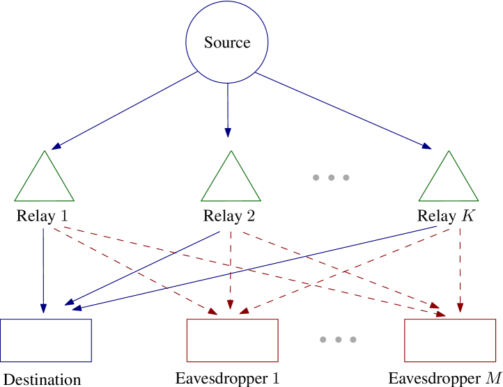
Figure 1: A diagram of secure AF relay networks with one source, one destination, $K$ relays, and $M$ eavesdroppers.

In the considered scenario, a source sends data to a destination through the assistance of $K$ relays that operate in the AF mode. In addition, there are $M$ eavesdroppers who want to intercept the information intended for the destination. It is assumed that there is no direct link between the source and the destination. The system model is illustrated in Fig. 1. We adopt the notations used in [46] for ease of discussion. Specifically, the channel between the source and relay $k$, and that between relay $k$ and the destination are denoted by $f_{k}$ and $g_{k}$, respectively. The channel between relay $k$ and eavesdropper $m$ is denoted by $h_{km}$. Let $w_{k}$ be the complex weight used at relay $k$. For notational convenience, the following vectors are defined: $\mathbf{g}\triangleq[g_{1},g_{2},\ldots,g_{K}]^{\mbox{\scriptsize H}}\in\mathbb{C}^{K\times 1}$, $\mathbf{h}_{m}\triangleq[h_{1m},h_{2m},\ldots,h_{Km}]^{\mbox{\scriptsize H}}\in\mathbb{C}^{K\times 1}$, $\mathbf{f}\triangleq[f_{1},f_{2},\ldots,f_{K}]^{\mbox{\scriptsize T}}\in\mathbb{C}^{K\times 1}$, and $\mathbf{w}\triangleq[w_{1},w_{2},\ldots,w_{K}]^{\mbox{\scriptsize T}}\in\mathbb{C}^{K\times 1}$. Let $\mathbf{n}_{\mathrm{r}}\sim\mathcal{CN}(0,\sigma^{2}\mathbf{I}_{K})$ be the noise vector at the relays. With the above notations, the signals received at the destination and eavesdropper $m$ are

$$y_{\mathrm{d}} = \sqrt{P_{\mathrm{s}}}\mathbf{g}^{\mbox{\scriptsize H}}\operatorname{\mathsf{D}}(\mathbf{f})\mathbf{w}s+\mathbf{n}_{\mathrm{r}}^{\mbox{\scriptsize T}}\operatorname{\mathsf{D}}^{\mbox{\scriptsize H}}(\mathbf{g})\mathbf{w}+n_{\mathrm{d}}$$ (12)

and

$$y_{\mathrm{e},m}=\sqrt{P_{\mathrm{s}}}\mathbf{h}_{m}^{\mbox{\scriptsize H}}\operatorname{\mathsf{D}}(\mathbf{f})\mathbf{w}s+\mathbf{n}_{\mathrm{r}}^{\mbox{\scriptsize T}}\operatorname{\mathsf{D}}^{\mbox{\scriptsize H}}(\mathbf{h}_{m})\mathbf{w}+n_{\mathrm{e},m}$$ (13)

respectively, where $P_{\mathrm{s}}$ is the transmit power at the source, $\operatorname{\mathsf{D}}(\mathbf{x})$ denotes the diagonal matrix with elements $\mathbf{x}$, $n_{\mathrm{d}}\sim\mathcal{CN}(0,\sigma^{2})$ and $n_{\mathrm{e},m}\sim\mathcal{CN}(0,\sigma^{2})$ are the noise at the destination and eavesdropper $m$, respectively. Then, the SINRs at the destination and eavesdropper $m$ are given by

$$\gamma_{\mathrm{d}}=\frac{\mathbf{w}^{\mbox{\scriptsize H}}\mathbf{A}\mathbf{w}}{\mathbf{w}^{\mbox{\scriptsize H}}\mathbf{G}\mathbf{w}+1},\;\textrm{and}\ \gamma_{\mathrm{e},m}=\frac{\mathbf{w}^{\mbox{\scriptsize H}}\mathbf{B}_{m}\mathbf{w}}{\mathbf{w}^{\mbox{\scriptsize H}}\mathbf{H}_{m}\mathbf{w}+1}$$ (14)

respectively, where $\mathbf{A}\triangleq(P_{\mathrm{s}}/\sigma^{2})\operatorname{\mathsf{D}}^{\mbox{\scriptsize H}}(\mathbf{f})\mathbf{gg}^{\mbox{\scriptsize H}}\operatorname{\mathsf{D}}(\mathbf{f})$, $\mathbf{G}\triangleq\operatorname{\mathsf{D}}(\mathbf{g})\operatorname{\mathsf{D}}^{\mbox{\scriptsize H}}(\mathbf{g})$, $\mathbf{B}_{m}\triangleq(P_{\mathrm{s}}/\sigma^{2})\operatorname{\mathsf{D}}^{\mbox{\scriptsize H}}(\mathbf{f})\mathbf{h}_{m}\mathbf{h}_{m}^{\mbox{\scriptsize H}}\operatorname{\mathsf{D}}(\mathbf{f})$, and $\mathbf{H}_{m}\triangleq\operatorname{\mathsf{D}}(\mathbf{h}_{m})\operatorname{\mathsf{D}}^{\mbox{\scriptsize H}}(\mathbf{h}_{m})$. Now the problem of maximizing the secrecy rate reads

$$\underset{\mathbf{w}}{\operatorname*{maximize}} \;\underset{1\leq m\leq M}{\min}\left(\log(1+\gamma_{\mathrm{d}})-\log(1+\gamma_{\mathrm{e},m})\right)$$ (15a)

$$\operatorname*{subject\leavevmode\nobreak\ to} \;\mathbf{w}^{\mbox{\scriptsize H}}\mathbf{C}\mathbf{w}\leq P_{\mathrm{tot}},\;\mathbf{w}^{\mbox{\scriptsize H}}\operatorname{\mathsf{D}}(\mathbf{e}_{k})\mathbf{C}\mathbf{w}\leq P_{k},\,\forall k$$ (15b)

where $\mathbf{C}\triangleq P_{\mathrm{s}}\operatorname{\mathsf{D}}^{\mbox{\scriptsize H}}(\mathbf{f})\operatorname{\mathsf{D}}(\mathbf{f})+\sigma^{2}\mathbf{I}_{K}$, $\mathbf{e}_{k}\triangleq[\underset{k-1}{\underbrace{0,\ldots,0}},1,\underset{K-k}{\underbrace{0,\ldots,0}}]$, $P_{\mathrm{tot}}$ is the maximum total transmit power for all the relays, and $P_{k}$ is the maximum transmit power for relay $k$.

To solve (15), [46] introduced the PSD matrix $\mathbf{W}\triangleq\mathbf{w}\mathbf{w}^{\mbox{\scriptsize H}}$ and arrived at a relaxation of this problem where the rank-1 constraint on $\mathbf{W}$ was dropped for tractability. Then the relaxed program was solved by a method involving two-stage optimization; a one-dimensional search was performed at the outer-stage and SDPs were solved at the inner-stage.

IV-B Proposed SOCP-based Solution

We now solve (15) based on the proposed approximations presented in the previous section. To do so, we first transform (15) into an equivalent formulation as

$$\underset{\mathbf{w},\alpha>0,\beta>0}{\operatorname*{minimize}} \;\frac{\beta}{\alpha}$$ (16a)

$$\operatorname*{subject\leavevmode\nobreak\ to} \;\frac{\mathbf{w}^{\mbox{\scriptsize H}}(\mathbf{A}+\mathbf{G})\mathbf{w}+1}{\mathbf{w}^{\mbox{\scriptsize H}}\mathbf{G}\mathbf{w}+1}\geq\alpha$$ (16b)

$$\;\frac{\mathbf{w}^{\mbox{\scriptsize H}}(\mathbf{B}_{m}+\mathbf{H}_{m})\mathbf{w}+1}{\mathbf{w}^{\mbox{\scriptsize H}}\mathbf{H}_{m}\mathbf{w}+1}\leq\beta,\;\forall m$$ (16c)

$$\;\mathbf{w}^{\mbox{\scriptsize H}}\mathbf{C}\mathbf{w}\leq P_{\mathrm{tot}},\;\mathbf{w}^{\mbox{\scriptsize H}}\operatorname{\mathsf{D}}(\mathbf{e}_{k})\mathbf{C}\mathbf{w}\leq P_{k},\forall k$$ (16d)

In fact, (16) is an epigraph form of (15) assuming the optimal value of the latter is strictly positive. Regarding (16), the objective function can be approximated using the upper bound in (App3), while the constraints (16b) and (16c) can be approximated by (App4) and (App6), respectively. The resulting convexified subproblem is an SOCP.

To complete the first application, we now provide the worst-case computational complexity of the proposed SOCP-based method and the SDP-based solution in [46], using the results in [31]. For the former, the worst-case arithmetic cost per iteration is $\mathcal{O}\bigl{(}K^{3}M(K+M)^{0.5}\bigr{)}$ which reduces to $\mathcal{O}\bigl{(}K^{3.5}\bigr{)}$ when $K\gg M$. For the latter, the worst-case per-iteration computational cost is $\mathcal{O}\left(K^{4}(M+K)^{0.5}(M+K^{2})\right)$ reducing to $\mathcal{O}\left(K^{6.5}\right)$ when $K\gg M$. The analysis implies that the per-iteration complexity of the proposed solution is much less sensitive to $K$ than that in [46]. We recall that the optimization method in [46] is also an iterative procedure. In addition, the complexity of each subproblem in the proposed method is much less than that in [46] (in orders of magnitude). Thus, we can reasonably expect that the proposed solution is superior to the SDP-based method in [46] in terms of numerical efficiency, which will be elaborated by numerical experiments in the following.

IV-C Numerical Results

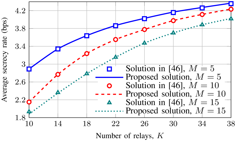
(a) Average secrecy rate (in bps).

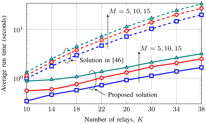
(b) Average run time (in seconds).

Figure 2: Average secrecy rate and average run time of the proposed solution and the solution in [46] versus different numbers of relays, $K$. We take the number of eavesdroppers, $M$, as $5$, $10$, and $15$.

We now numerically evaluate the performances of the proposed solution in terms of achieved secrecy rate and computational complexity (i.e. run time). The considered simulation model follows the one in [46]. Specifically, the channels are independent Rayleigh fading with zero means and unit variances. The noise variance is set to $\sigma^{2}=1$. The transmit power at the source is $P_{\mathrm{s}}=20$ dB, the maximum total transmit power at the relays is $P_{\textrm{tot}}=15$ dB, and the power budget at antenna $k$ is determined as $P_{k}=P_{\textrm{tot}}/2K$ if $k$ is odd and $P_{k}=2P_{\textrm{tot}}/K$ otherwise. We note that a feasible $(\mathbf{w},\alpha,\beta)$ can be easily generated as follows. First, a random (but small enough) $\mathbf{w}$ is generated satisfying (16d). Then, the left sides of the constraints (16b) and (16c) are computed accordingly, from which feasible $\alpha$ and $\beta$ can be found easily.

In Fig. 2(a), we plot the achieved secrecy rate (in bits per second) of the considered schemes with different numbers of relays and eavesdroppers. We can observe that, in all cases, the proposed SOCP-based solution achieves nearly the same performance as the SDP-based solution in [46], but with much lower computation time as shown in Fig. 2(b). As expected, the run time of the proposed solution increases slowly with $M$ and $K$ compared to that of the existing method. In particular, the computation time improvement achieved by the proposed solution is huge for large numbers of relays and eavesdroppers (approximately 10 times faster in favor of the proposed method at $K=38$). This observation is consistent with the theoretical bounds of the arithmetical cost reported in the previous subsection.

V Application II: Beamforming Designs for Cognitive Radio Multicasting

We now turn our attention to the cognitive radio which has been considered as one of the most promising techniques to improve the spectrum utilization. In particular, we revisit the problem of transmit power minimization for secondary multicasting investigated in [21].

V-A System Model and Problem Formulation

The considered system model consists of a secondary multi-antenna base station transmitting data to $G$ groups of secondary single-antenna users where users in the same group receive the same information content. Let $\mathcal{U}_{g}$, $g=1,...,G$, denote the set of users in group $g$. The total number of secondary users is $M$, and each user belongs to only one group. In addition, there exist $L$ primary single-antenna users who are interfered by the secondary transmission. A diagram of the considered system is shown in Fig. 3. Let $N$ be the number of antennas equipped at the secondary BS, $\mathbf{h}_{i}\in\mathbb{C}^{1\times N}$ be the channel (row) vector between the secondary BS and secondary user (SU) $i$, $\mathbf{l}_{j}\in\mathbb{C}^{1\times N}$ be the channel vector between the secondary BS and primary user (PU) $j$, and $\mathbf{x}_{g}\in\mathbb{C}^{N\times 1}$ be the multicast transmit beamforming vector at the secondary BS for group $g$. The problem of minimizing the transmit power at the secondary BS is stated as [21]

$$\underset{\{\mathbf{x}_{g}\}_{g=1}^{G}}{\operatorname*{minimize}} \;\sum_{g=1}^{G}||\mathbf{x}_{g}||_{2}^{2}$$ (17a)

$$\operatorname*{subject\leavevmode\nobreak\ to} \;\frac{|\mathbf{h}_{i}\mathbf{x}_{g}|^{2}}{\sum_{k\neq g}|\mathbf{h}_{i}\mathbf{x}_{k}|^{2}+\sigma_{i}^{2}}\geq\alpha_{i},\forall i\in\mathcal{U}_{g},g=1,...,G$$ (17b)

$$\;\sum_{g=1}^{G}|\mathbf{l}_{j}\mathbf{x}_{g}|^{2}\leq\beta_{j},\;\forall j=1,...,L$$ (17c)

where $\beta_{j}$ is the predefined interference threshold at PU $j$, $\alpha_{i}$ and $\sigma_{i}^{2}$ are the QoS level and noise variance corresponding to SU $i$, respectively. The constraints in (17b) guarantee the QoSs of the SUs while those in (17c) ensure that the interference generated by the secondary transmission at the PUs are smaller than predefined thresholds.

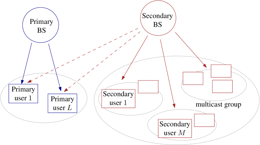
Figure 3: An example of cognitive multicast transmissions with $L$ PUs and multiple multicast groups including total $M$ SUs.

Problem (17) is a nonconvex program, and the prevailing approach is to lift the problem into a SDP [47, 48], i.e. PSD matrices $\mathbf{X}_{g}=\mathbf{x}_{g}\mathbf{x}_{g}^{\mbox{\scriptsize H}}$, $\forall g$, are introduced and the rank-1 constraints on $\{\mathbf{X}_{g}\}_{g=1}^{G}$ are ignored. However, this approach cannot guarantee even a feasible solution, since the relaxed problem generally does not yield rank-1 solutions and randomization procedures are inefficient. To overcome this shortcoming, [21] proposed an iterative approach where the PSD matrices $\{\mathbf{X}_{g}\}_{g=1}^{G}$ were still introduced. However, the noncovex rank-1 constraints (which were expressed a reverse convex constraint, i.e. $\sum_{g=1}^{G}\operatorname{tr}(\mathbf{X}_{g})-\lambda_{\max}(\mathbf{X}_{g})\leq 0$ where $\lambda_{\max}(\mathbf{X}_{g})$ is the maximal eigenvalue of $\mathbf{X}_{g}$) were sequentially approximated in a manner similar to the SCA framework presented in this paper.

V-B Proposed SOCP-based Solution

We observe that the objective function in (17a) and constraint in (17c) are convex. Thus the difficulty of solving the problem comes from the nonconvex constraints in (17b). To handle these constraints, let us introduce $\mathbf{x}\triangleq[\mathbf{x}_{1};...;\mathbf{x}_{G}]$ and equivalently rewrite (17) as

$$\underset{\mathbf{x}}{\operatorname*{minimize}} \;||\mathbf{x}||_{2}^{2}$$ (18a)

$$\operatorname*{subject\leavevmode\nobreak\ to} \;\frac{\mathbf{x}^{\mbox{\scriptsize H}}\hat{\mathbf{H}}_{i}\mathbf{x}}{\mathbf{x}^{\mbox{\scriptsize H}}\bar{\mathbf{H}}_{i}\mathbf{x}+\sigma_{i}^{2}}\geq\alpha_{i},\forall i\in\mathcal{U}_{g},g=1,...,G$$ (18b)

$$\;\mathbf{x}^{\mbox{\scriptsize H}}\mathbf{L}_{j}\mathbf{x}\leq\beta_{j},\;\forall j$$ (18c)

where $\hat{\mathbf{H}}_{i}=\operatorname{blkdiag}(\boldsymbol{0},\mathbf{H}_{i},\boldsymbol{0})$, $\mathbf{H}_{i}\triangleq\mathbf{h}_{i}^{\mbox{\scriptsize H}}\mathbf{h}_{i}$, $\bar{\mathbf{H}}_{i}=\operatorname{blkdiag}(\underbrace{\mathbf{H}_{i},\ldots\mathbf{H}_{i}}_{g-1\textrm{ terms}},\mathbf{0},\underbrace{\mathbf{H}_{i},\ldots\mathbf{H}_{i}}_{G-g\textrm{ terms}})$ (for $i\in\mathcal{U}_{g}$), and $\mathbf{L}_{j}=\operatorname{blkdiag}(\underbrace{\mathbf{l}_{j}^{\mbox{\scriptsize H}}\mathbf{l}_{j},\ldots\mathbf{l}_{j}^{\mbox{\scriptsize H}}\mathbf{l}_{j}}_{G\textrm{ terms}})$. Now, we can easily use (App4) to deal with (18b), and the convex approximated problem is actually an SOCP. We remark that, for (17), it is nontrivial to find a feasible $\{\mathbf{x}_{g}\}_{g=1}^{G}$ to start the SCA procedure. Thus the relaxed version, i.e. Algorithm 2, is invoked for some first iterations, until a feasible point is found.

We now compare the complexity of the proposed solution and the method in [21]. In particular, the worst-case complexity for solving the SOCP in (18) is $\mathcal{O}\left(G^{3}N^{3}(M+L)^{1.5}\right)$, while that for the SDP in [21] is $\mathcal{O}\left(G^{2}N^{4}(M+L+GN)^{0.5}(M+L+GN^{2})\right)$. When the number of transmit antennas at the secondary BS is large, the two bounds reduce to $\mathcal{O}\left(N^{3}\right)$ and $\mathcal{O}\left(N^{6.5}\right)$, respectively.

V-C Numerical Results

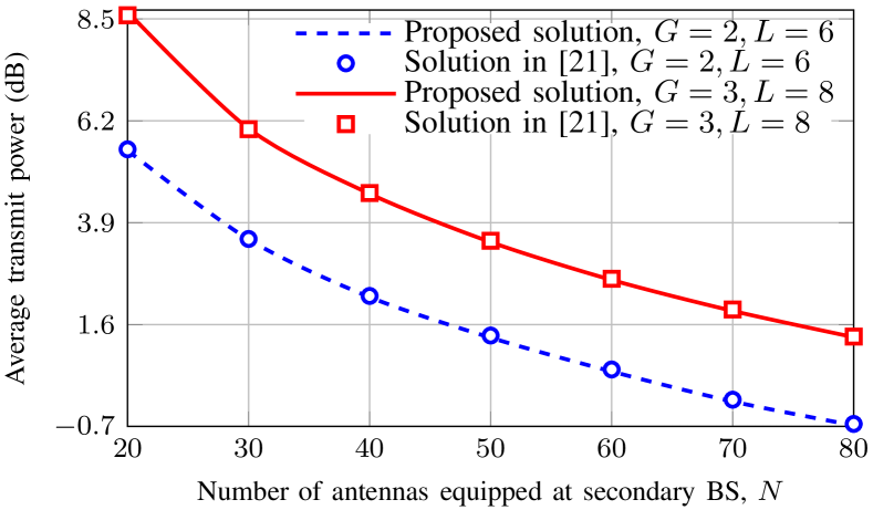
(a) Average transmit power at the secondary BS (in dB).

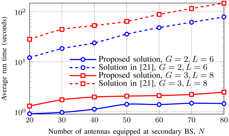
(b) Average run time (in seconds).

Figure 4: Average transmit power at the secondary BS and average run time of the proposed solution and the solution in [21] versus the number of equipped antennas, $N$. Two sets of $(G,L)$ are taken those are $(2,6)$ and $(3,8)$. Each multicast group includes 4 secondary users.

We follow the simulation model considered in [21] for performance comparisons. Particularly, the channels are generated as $\mathbf{h}_{i}\thicksim\mathcal{CN}(0,\mathbf{I}_{N})$, $\mathbf{l}_{j}\thicksim\mathcal{CN}(0,\mathbf{I}_{N})$. The QoS levels at the SUs and the interference thresholds at the PUs are set to $\alpha_{i}=10\;\textrm{dB}$, $\forall i$ and $\beta_{j}=5\;\textrm{dB},$ $\forall j$. The stopping criterion of the method in [21] is when the decrease in the last 5 iterations is smaller than $10^{-3}$.

In Fig. 4(a), we plot the average required transmit power at the secondary BS for the proposed method and the one in [21] as functions of the number of transmit antennas $N$. As can be seen, the transmit powers required by the two schemes are almost the same for all considered scenarios. In other words, the proposed solution is similar to the one in [21] in terms of power efficiency. However, the proposed method is much more computationally efficient as demonstrated in Fig. 4(b), in which we plot the run time of the two methods. We can clearly see that the average run time of both schemes increases with $N$, but slowly for the proposed solution and very rapidly for the method in [21]. As a result, the computation time of the method in [21] is much higher than that of the proposed solution, especially for large $N$. This numerical observation is consistent with the complexity analysis provided in the preceding subsection. In summary, the numerical results in Fig. 4 demonstrate that the proposed SOCP-based solution is superior to the existing one presented in [21].

VI Application III: Precoding Design for MIMO Relaying

Relay-assisted wireless communications is expected to play a key role in improving coverage and spectral efficiency for the current and future generations of cellular networks. In this section, we apply the proposed approximations to the scenario of multiuser MIMO relaying which was investigated in [49].

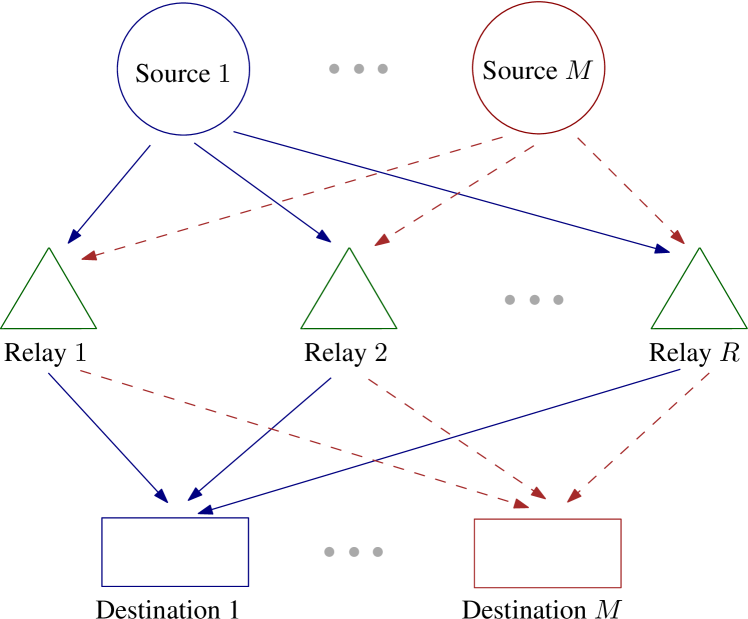
Figure 5: An example of relaying communications with $M$ source-destination pairs and $R$ MIMO relays. The transmissions follow the two-phase precode-and-forward principle.

VI-A System Model and Problem Formulation

We consider the wireless communication scenario in which the transmission of $M$ source-destination pairs are simultaneously assisted by a set of $R$ relays. Each of the sources and destinations is equipped with single antenna, whereas each relay is equipped with $N_{\mathrm{R}}$ antennas (the total number of antennas at the relays is $N=RN_{\mathrm{R}}$). Suppose there are no direct links between the sources and destinations, and the relays operate according to the AF protocol. That is, the sources transmit their information to the relays in the first phase, and then the relays process the received signals and retransmit them to the destinations in the second phase. The considered system model is illustrated in Fig. 5. We reuse the notations introduced in [49]. Specifically, let $\mathbf{s}=[s_{1},s_{2},...,s_{M}]^{\mbox{\scriptsize T}}\in\mathbb{C}^{M\times 1}$, where $E[|s_{i}|^{2}]=\sigma_{\mathrm{s}}^{2}$, be the vector of messages sent by the sources, $\mathbf{h}_{i}=[h_{i1},h_{i2},...,h_{iN}]^{\mbox{\scriptsize T}}\in\mathbb{C}^{N\times 1}$ and $\mathbf{l}_{i}=[l_{i1},l_{i2},...,l_{iN}]^{\mbox{\scriptsize T}}\in\mathbb{C}^{N\times 1}$ be the vectors of channels from source $i$ to the relays and from the relays to destination $i$, respectively. Let $\mathbf{X}_{k}\in\mathbb{C}^{N_{\mathrm{R}}\times N_{\mathrm{R}}}$ be the processing matrix at relay $k$, $k=1,...,R$. For ease of description, we also define $\mathbf{H}\triangleq[\mathbf{h}_{1},\mathbf{h}_{2},...,\mathbf{h}_{M}]$, $\mathbf{L}\triangleq[\mathbf{l}_{1},\mathbf{l}_{2},...,\mathbf{l}_{M}]$, and $\mathbf{X}\triangleq\mathrm{blkdiag}\{\mathbf{X}_{k}\}_{k}$ as in [49]. Then the signal vectors received at the relays and destination $i$ are given by

$$\mathbf{y}_{\mathrm{up}}=\mathbf{Hs}+\mathbf{n}_{\mathrm{re}}$$ (19)

and

$$y_{\mathrm{de},i}=\mathbf{l}_{i}^{\mbox{\scriptsize T}}\mathbf{X}\mathbf{h}_{i}s_{i}+\sum_{j\neq i}\mathbf{l}_{i}^{\mbox{\scriptsize T}}\mathbf{X}\mathbf{h}_{j}s_{j}+\mathbf{l}_{i}^{\mbox{\scriptsize T}}\mathbf{X}\mathbf{n}_{\mathrm{re}}+n_{\mathrm{de},i}$$ (20)

respectively, where $\mathbf{n}_{\mathrm{re}}\thicksim\mathcal{CN}(0,\sigma_{\mathrm{re}}^{2}\mathbf{I}_{N})$ and $n_{\mathrm{de},i}\thicksim\mathcal{CN}(0,\sigma_{\mathrm{de}}^{2})$ are the noise vectors at the relays and destination $i$. Accordingly, the SINR at the $i$th destination is written as

$$\gamma_{i}(\mathbf{X})=\frac{\sigma_{\mathrm{s}}^{2}|\mathbf{l}_{i}^{\mbox{\scriptsize H}}\mathbf{X}\mathbf{h}_{i}|^{2}}{\sigma_{\mathrm{s}}^{2}\sum_{j\neq i}|\mathbf{l}_{i}^{\mbox{\scriptsize H}}\mathbf{X}\mathbf{h}_{j}|^{2}+\sigma_{\mathrm{re}}^{2}\left\|\mathbf{X}^{\mbox{\scriptsize H}}\mathbf{l}_{i}\right\|_{2}^{2}+\sigma_{\mathrm{de}}^{2}}$$ (21)

The power consumption at antenna $n$, $n=1,...,N$, is given by

$$P_{n}=\mathbf{e}_{n}\mathbf{X}\mathbf{B}\mathbf{X}^{\mbox{\scriptsize H}}\mathbf{e}_{n}^{\mbox{\scriptsize H}}$$ (22)

where $\mathbf{B}\triangleq\sigma_{\mathrm{s}}^{2}\mathbf{H}\mathbf{H}^{\mbox{\scriptsize H}}+\sigma_{\mathrm{re}}^{2}\mathbf{I}$, and $\mathbf{e}_{n}\triangleq[\underset{n-1}{\underbrace{0,\ldots,0}},1,\underset{N-n}{\underbrace{0,\ldots,0}}]$. Based on the above discussions, the problem of max-min fairness data rate between the source-destination pairs under the power constraint of each individual antenna at the relays reads [49]

$$\underset{\mathbf{X}}{\operatorname*{maximize}} \;\underset{1\leq i\leq M}{\min}\;\gamma_{i}(\mathbf{X})$$ (23a)

$$\operatorname*{subject\leavevmode\nobreak\ to} \;\mathbf{e}_{n}\mathbf{X}\mathbf{B}\mathbf{X}^{\mbox{\scriptsize H}}\mathbf{e}_{n}^{\mbox{\scriptsize H}}\leq\bar{P}_{n},\;\forall n=1,...,N$$ (23b)

where $\bar{P}_{n}$ is the maximum transmit power at antenna $n$. The left sides of constraints in (23b) are convex quadratic functions, since matrix $\mathbf{B}$ is positive definite. Thus the feasible set of (23) is convex. However, (23) is still intractable because $\gamma_{i}(\mathbf{X})$ is neither concave nor convex with respect to $\mathbf{X}$. To solve (23), [49] transformed it to a DC program where the resulting feasible set contains linear matrix inequalities (LMIs) and the objective is a DC function. After that, [49] applied the DCA to solve the DC program which results in an SDP in each iteration.

VI-B Proposed SOCP-based Solution

To apply the proposed approximations, let us define $\mathbf{x}\triangleq\operatorname{vec}(\mathbf{X})\in\mathbb{C}^{R^{2}N_{\mathrm{R}}^{2}}$ and rewrite the expression in (21) with respect to $\mathbf{x}$. To this end we recall two useful inequalities: $\operatorname{tr}(\mathbf{A}^{\mbox{\scriptsize H}}\mathbf{B})=\operatorname{vec}(\mathbf{A})^{\mbox{\scriptsize H}}\operatorname{vec}(\mathbf{B})$ and $\operatorname{vec}(\mathbf{A}\mathbf{B})=(\mathbf{I}_{n}\otimes\mathbf{A})\operatorname{vec}(\mathbf{B})$. Now it is easy to see that (21) is equivalent to

$$\gamma_{i}(\mathbf{x}) =\frac{\sigma_{\mathrm{s}}^{2}\mathbf{x}^{\mbox{\scriptsize H}}\bar{\mathbf{H}}_{ii}\mathbf{x}}{\sigma_{\mathrm{s}}^{2}\sum_{j\neq i}\mathbf{x}^{\mbox{\scriptsize H}}\bar{\mathbf{H}}_{ij}\mathbf{x}+\sigma_{\mathrm{re}}^{2}\mathbf{x}^{\mbox{\scriptsize H}}\tilde{\mathbf{L}}_{i}\mathbf{x}+\sigma_{\mathrm{de}}^{2}}$$

$$=\frac{\sigma_{\mathrm{s}}^{2}\mathbf{x}^{\mbox{\scriptsize H}}\bar{\mathbf{H}}_{ii}\mathbf{x}}{\mathbf{x}^{\mbox{\scriptsize H}}\tilde{\mathbf{H}}_{i}\mathbf{x}+\sigma_{\mathrm{de}}^{2}}$$ (24)

where $\bar{\mathbf{H}}_{ij}\triangleq\operatorname{vec}(\mathbf{l}_{i}\mathbf{h}_{j}^{\mbox{\scriptsize H}})\operatorname{vec}(\mathbf{l}_{i}\mathbf{h}_{j}^{\mbox{\scriptsize H}})^{\mbox{\scriptsize H}}$, $\tilde{\mathbf{L}}_{i}\triangleq(\mathbf{I}_{N}\otimes\mathbf{l}_{i}^{\mbox{\scriptsize H}})^{\mbox{\scriptsize H}}(\mathbf{I}_{N}\otimes\mathbf{l}_{i}^{\mbox{\scriptsize H}})$, and $\tilde{\mathbf{H}}_{i}\triangleq\sigma_{\mathrm{s}}^{2}\sum_{j\neq i}\bar{\mathbf{H}}_{ij}+\sigma_{\mathrm{re}}^{2}\tilde{\mathbf{L}}_{i}$. Based on above discussion, we can reformulate (23) using its epigraph form as

$$\underset{\mathbf{x},\vartheta>0}{\operatorname*{maximize}} \;\vartheta$$ (25a)

$$\operatorname*{subject\leavevmode\nobreak\ to} \;\gamma_{i}(\mathbf{x})\geq\vartheta,\;\forall i=1,...,M$$ (25b)

$$\;\mathbf{x}^{\mbox{\scriptsize H}}\tilde{\mathbf{B}}_{n}\mathbf{x}\leq\bar{P}_{n},\;\forall n=1,...,N.$$ (25c)

where $\tilde{\mathbf{B}}_{n}\triangleq(\mathbf{I}_{N}\otimes\mathbf{A}_{n})^{\mbox{\scriptsize H}}(\mathbf{B}^{\mbox{\scriptsize T}}\otimes\mathbf{I}_{N})$, $\mathbf{A}_{n}\triangleq\mathbf{e}_{n}\mathbf{e}_{n}^{\mbox{\scriptsize H}}$. Now, the nonconvex constraints in (25b) can be straightforwardly approximated by (App5).

The complexity analysis is as follows. We recall that the dimension of $\mathbf{x}$ in (25) is $R^{2}N_{\mathrm{R}}^{2}$, however the number of complex variables in $\mathbf{x}$ is only $RN_{\mathrm{R}}^{2}$ (other elements are zero according to the arrangement of $\mathbf{X}$). Therefore, assumming $RN_{\mathrm{R}}\gg M$, the worst-case complexity for solving (25) is $\mathcal{O}(R^{4.5}N_{\mathrm{R}}^{6.5})$. On the other hand, for the SDP considered in [49], the corresponding worst-case complexity is $\mathcal{O}(R^{6}N_{\mathrm{R}}^{8})$. Thus, the proposed SOCP-based approach achieves significant gains in terms of computation time over the SDP-based method in [49].

VI-C Numerical Results

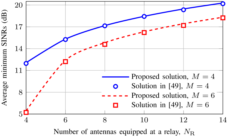
(a) Average achieved minimum SINR (in dB).

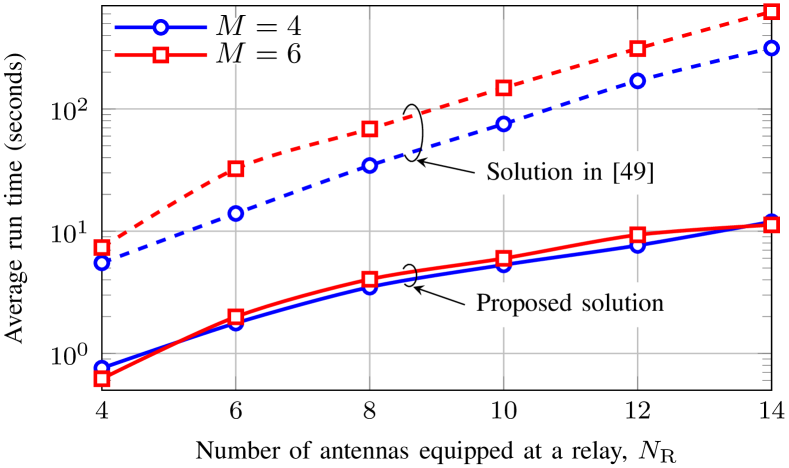
(b) Average run time (in seconds).

Figure 6: Average achieved minimum SINR and the computational costs (in terms of run time) of the proposed solution and the solution in [49] versus number of antennas equipped at a relay, $N_{\mathrm{R}}$. The number of source-destination pairs $M$ is taken as $4$ and $6$.

We evaluate the proposed solution in terms of run time and achieved minimum SINR using the system model studied in [49]. The channels are randomly generated as $\mathbf{h}_{i}\thicksim\mathcal{CN}(0,\mathbf{I}_{N})$, and $\mathbf{l}_{i}\thicksim\mathcal{CN}(0,\mathbf{I}_{N})$. The noise variances at the relays and destinations are set to $\sigma_{\mathrm{re}}^{2}=\sigma_{\mathrm{de}}^{2}=1$. The transmit power is $\sigma_{\mathrm{s}}^{2}=20$ dB for all the sources and the number of relays is $R=2$. We simply set the power budget $P_{\mathrm{R}}=10$ dB for all relays, and the maximum transmit power at each individual antenna is $\bar{P}_{n}=P_{\mathrm{R}}/N_{\mathrm{R}}$, $\forall n$. For this problem, a feasible initial point to (25) can be easily created by simple manipulations. That is, $\mathbf{x}^{(0)}$ is randomly generated and then rescaled, if required, to satisfy the power constraints in (23b). The iterative method in [49] terminates if the increase in the objective in the last 5 iterations is less than $10^{-3}$.

In Fig. 6(a) we compare the achieved minimum SINR of the proposed SOCP-based method and the SDP-based solution in [49] as functions of $N_{\mathrm{R}}$. We can observe that the minimum SINR performance of two methods of comparison is the same for all considered scenarios. However the method in [49] comes at the cost of much higher computational complexity which is shown in Fig. 6(b). In particular, Fig. 6(b) shows that the complexity of both methods increases with respect to $N_{\mathrm{R}}$. We can also see that the run time of the proposed solution is much smaller than that of the SDP-based solution. This observation agrees with the complexity analysis presented in the previous subsection.

VII Application IV: Power Management for Weighted Sum Rate Maximization and Max-mix Fairness Energy Efficiency in Multiuser Multicarrier Systems

In the last application, we apply the proposed approximations to solve the power control problems for maximizing weighted sum rate and energy efficiency fairness. While the former is a classical problem, the latter has been receiving growing attention in recent years for green wireless networks. The power control problem for weighted sum rate maximization (WSRmax) was studied in [50], using a GP method, while the one for energy efficiency fairness was recently studied in [51] using a generic NLP approach. We will show in the following that these two important problems can be simply solved by the proposed conic quadratic formulations.

VII-A System Model and Problem Formulation

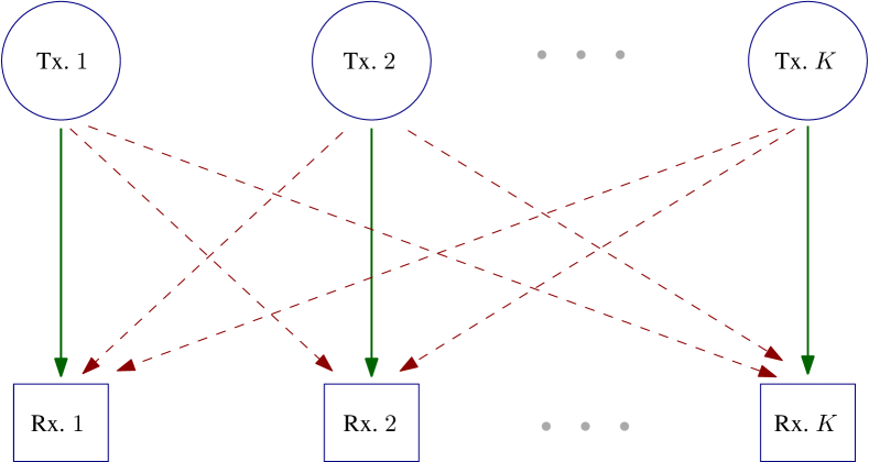
Figure 7: A diagram of multiuser multicarrier systems. The transmitters and receivers are labeled as Tx. and $\textrm{Rx}.$, respectively. The green (solid) lines represent the desire signals, while the red (dashed) ones denote the interference from other transmitters. The lines in the figure represent one of $N$ independent subcarriers.

Consider a general network of $K$ communication links where each of the transmitters and receivers is equipped with a single antenna as illustrated in Fig. 7. This system model has been the subject in many works such as [50, 51, 41, 42, 52]. For the ease of discussion, we follow the notations used in [50]. The $k$th transmitter sends its data to the $k$th receiver through $N$ independent subcarriers. The channel gain between transmitter $l$ and receiver $k$ over carrier $n$ is denoted by $G_{kln}$. We note that this setup is a generalization of the system model studied in [41, 42] where $N=1$. The interference at each receiver is treated as background noise. Accordingly, the achievable data rate of the $k$th link is given by

$$R_{k}=\sum_{n=1}^{N}\log\biggl{(}1+\frac{G_{kkn}p_{kn}}{\sigma^{2}+\sum_{l\neq k}G_{kln}p_{ln}}\biggr{)}$$ (26)

where $p_{kn}$ is the amount of power allocated to the $n$th carrier at the $k$th transmitter, and $\sigma^{2}$ denotes the noise variance.

VII-A1 Weighted Sum Rate Maximization

The WSRmax problem is given by [50, 52]

$$\underset{\mathbf{p}}{\operatorname*{maximize}} \;\sum_{k=1}^{K}w_{k}R_{k}$$ (27a)

$$\operatorname*{subject\leavevmode\nobreak\ to} \;\sum_{n=1}^{N}p_{kn}\leq\bar{p}_{k},\,\forall k;\;0\leq p_{kn}\leq\bar{p}_{kn},\,\forall k,n.$$ (27b)

where $w_{k}$ is the weight associated with the $k$th user, $\bar{p}_{k}$ is the maximum transmit power at transmitter $k$ and $\bar{p}_{kn}$ is the power spectrum mask. It is known that (27) is NP-hard [13], and [50] and [52] applied an SCA approach to solve this problem. In particular, [50] approximated the WSRmax problem as a sequence of GPs. As discussed in [50] the GP-based method suffers some numerical difficulties.

VII-A2 Energy Efficiency Fairness

The problem of max-min energy efficiency fairness (maxminEEfair) for the multiuser multicarrier system has been considered in many recent works such as [51, 42] which is stated as

$$\underset{\mathbf{p}}{\operatorname*{maximize}} \;\underset{1\leq k\leq K}{\min}\;\frac{R_{k}}{\sum_{n=1}^{N}p_{kn}+p_{k}^{\mathrm{c}}}$$ (28a)

$$\operatorname*{subject\leavevmode\nobreak\ to} \;\sum_{n=1}^{N}p_{kn}\leq\bar{p}_{k},\,\forall k;\;0\leq p_{kn}\leq\bar{p}_{kn},\,\forall k,n.$$ (28b)

where $p_{k}^{\mathrm{c}}$ is a constant that denotes the total circuit power consumption for the link between the $k$th transmitter and the $k$th receiver. To solve (28), [51] proposed a two-stage iterative method which is a combination of modified Dinkelbach’s algorithm and the SCA technique. More specifically, the SCA framework is applied to arrive at a max-min concave-convex fractional program which is solved by the modified Dinkelbach method. We note that the work of [51] used the same approximations introduced in [50, 52, 43] to deal with the nonconvexity of $R_{k}$. However, the convex problem achieved at each iteration of their proposed iterative method is a generic NLP.

VII-B Proposed SOCP-based Solutions

VII-B1 Proposed Solution for WSRmax

Using the epigraph form we can equivalently rewrite (27) as

$$\underset{\mathbf{p},\mathbf{t}\geq 1}{\operatorname*{maximize}} \;\sum_{k=1}^{K}w_{k}\sum_{n=1}^{N}\log t_{kn}$$ (29a)

$$\operatorname*{subject\leavevmode\nobreak\ to} \;\frac{\sigma_{kn}^{2}+\sum_{l=1}^{K}G_{kln}p_{ln}}{\sigma_{kn}^{2}+\sum_{l\neq k}G_{kln}p_{ln}}\geq t_{kn},\,\forall k,n$$ (29b)

$$\sum_{n=1}^{N}p_{kn}\leq\bar{p}_{k},\,\forall k;\;0\leq p_{kn}\leq\bar{p}_{kn},\,\forall k,n.$$ (29c)

It is obvious that (App1) and (App2) can be used to handle (29b), but this does not lead to an SOCP immediately due to the fact that the cost function in (29a) is not in a quadratic form at hand. However, if $w_{k}=1$ for all $k$ (i.e., the sum rate maximization problem), then the objective in (29a) can be replaced by the geometric mean of $t_{kn}$’s, which is SOC representable [30], and the resulting problem becomes an SOCP. For the general case of $w_{k}$’s, we can rewrite (27) as

$$\underset{\mathbf{p},\mathbf{t}\geq 0}{\operatorname*{maximize}} \;\sum_{k=1}^{K}w_{k}\sum_{n=1}^{N}t_{kn}$$ (30a)

$$\operatorname*{subject\leavevmode\nobreak\ to} \;u_{kn}\log\frac{u_{kn}}{\tilde{u}_{kn}}\geq u_{kn}t_{kn},\,\forall k,n$$ (30b)

$$\sum_{n=1}^{N}p_{kn}\leq\bar{p}_{k},\,\forall k;\;0\leq p_{kn}\leq\bar{p}_{kn},\,\forall k,n.$$ (30c)

where $u_{kn}\triangleq\sigma_{kn}^{2}+\sum_{l=1}^{K}G_{kln}p_{ln}$ and $\tilde{u}_{kn}\triangleq\sigma_{kn}^{2}+\sum_{l\neq k}G_{kln}p_{ln}$. Note that $u_{kn}$ and $\tilde{u}_{kn}$ are not newly introduced variables but affine expressions of $p_{kn}$’s. We remark that $u_{kn}\log\frac{u_{kn}}{\tilde{u}_{kn}}$ is jointly convex with $u_{kn}$ and $\tilde{u}_{kn}$. Thus, in light of the SCA framework, we can approximate the left hand side in (30b) using the first order and the right hand side using (App1) or (App2), which results in an SOCP.

The proposed method described above introduces $KN$ additional auxiliary variables, which has a detrimental impact on the overall complexity for large-scale problems. For (29), we are able to arrive at a more efficient formulation. The idea is that since the feasible set of (27) is defined by linear constraints, we can approximate the objective by a quadratic function based on the Lipschitz continuity to arrive at a QP. This approximation method has been briefly discussed in Section II-D and will be elaborated in the following. Let us rewrite (27) as

$$\underset{\mathbf{p},\mathbf{t}}{\operatorname*{minimize}} \;f(\mathbf{p},\mathbf{t})\triangleq-\sum_{k=1}^{K}w_{k}\sum_{n=1}^{N}\log\Bigl{(}1+\frac{p_{kn}}{t_{kn}}\Bigr{)}$$ (31a)

$$\operatorname*{subject\leavevmode\nobreak\ to} \;t_{kn}=\tilde{\sigma}_{kn}^{2}+\sum_{l\neq k}\tilde{G}_{kln}p_{ln},\,\forall k,n;\eqref{eq:mcpowerconstraint}$$ (31b)

where $\mathbf{t}\triangleq\{t_{kn}\}_{k,n}$, $\tilde{\sigma}_{kn}^{2}=\sigma^{2}/G_{kkn}$ and $\tilde{G}_{kln}=G_{kln}/G_{kkn}$ for $l\neq k$. For mathematical exposition, we temporarily treat $\mathbf{t}$ as a vector of newly introduced variables. It implicitly holds that $0<\tilde{\sigma}_{kn}^{2}\leq t_{kn}\leq\tilde{\sigma}_{kn}^{2}+\sum_{l\neq k}\tilde{G}_{kln}\bar{p}_{ln}$, $\forall k,n$. In particular, we have the following lemma.

Lemma 1.

Consider the function $f(x,y)=\log(1+\frac{x}{y})$ over the domain $D=\{(x,y)|x\geq x_{0}\geq 0,y\geq y_{0}>0\}$. Then the Hessian of $f(x,y)$ satisfies $\nabla^{2}f(x,y)+\rho\mathbf{I}_{2}\succeq\boldsymbol{0}$ for $\rho\geq\rho_{0}=(x_{0}+y_{0})^{-2}$.

Proof:

The Hessian of $f(x,y)$ is given by

$$\nabla^{2}f(x,y)=\left[\begin{array}[]{cc}-\frac{1}{(x+y)^{2}}&\frac{-1}{(x+y)^{2}}\\ \frac{-1}{(x+y)^{2}}&\frac{x(x+2y)}{(xy+y^{2})^{2}}\end{array}\right]\\ =\frac{1}{(x+y)^{2}}\left[\begin{array}[]{cc}-1&-1\\ -1&\frac{x(x+2y)}{y}\end{array}\right]$$ (32)

It is easy to see that since $x\geq x_{0}$ and $y>y_{0}$, $\nabla^{2}f(x,y)+\rho\mathbf{I}_{2}\succeq\boldsymbol{0}$ for $\rho\geq\rho_{0}(x_{0}+y_{0})^{-2}$, which completes the proof. Lemma 1 implies that the function $\log(1+\frac{x}{y})+\rho x^{2}+\rho y^{2}$ is convex for $\rho\geq\rho_{0}$. As a result, we can rewrite the objective function in (31) as the following DC function

$$f(\mathbf{p},\mathbf{t})=h(\mathbf{p},\mathbf{t})-g(\mathbf{p},\mathbf{t})$$ (33)

where $h(\mathbf{p},\mathbf{t})\triangleq\sum_{k=1}^{K}w_{k}\sum_{n=1}^{N}\rho_{kn}(p_{kn}^{2}+t_{kn}^{2})$ and $g(\mathbf{p},\mathbf{t})\triangleq\sum_{k=1}^{K}w_{k}\sum_{n=1}^{N}\rho_{kn}(p_{kn}^{2}+t_{kn}^{2})+\log\Bigl{(}1+\frac{p_{kn}}{t_{kn}}\Bigr{)}$ are both convex. The values of $\rho_{kn}$’s are determined based on Lemma 1. In light of the SCA-based approach, a convex upper bound of $f(\mathbf{p},\mathbf{t})$ is given by

$$f(\mathbf{p},\mathbf{t})\leq F(\mathbf{p},\mathbf{t};\tilde{\mathbf{p}},\tilde{\mathbf{t}})\triangleq h(\mathbf{p},\mathbf{t})-g(\tilde{\mathbf{p}},\tilde{\mathbf{t}})\\ -\bigl{\langle}\bigl{[}\nabla_{\mathbf{p}}g(\tilde{\mathbf{p}},\tilde{\mathbf{t}});\nabla_{\mathbf{t}}g(\tilde{\mathbf{p}},\tilde{\mathbf{t}})\bigr{]}^{\mbox{\scriptsize T}},\bigl{[}\mathbf{p}-\tilde{\mathbf{p}};\mathbf{t}-\tilde{\mathbf{t}}\bigr{]}\bigr{\rangle}$$ (34)

which is a quadratic function. Consequently, the problem considered in the $\theta$th iteration of the SCA-based approach is given by

$$\underset{\mathbf{p},\mathbf{t}}{\operatorname*{minimize}} \;\tilde{f}(\mathbf{p},\mathbf{t})\triangleq F(\mathbf{p},\mathbf{t};\mathbf{p}^{(\theta-1)},\mathbf{t}^{(\theta-1)})$$ (35a)

$$\operatorname*{subject\leavevmode\nobreak\ to} \;t_{kn}=\tilde{\sigma}_{kn}^{2}+\sum_{l\neq k}\tilde{G}_{kln}p_{ln},\,\forall k,n$$ (35b)

$$\;\sum_{n=1}^{N}p_{kn}\leq\bar{p}_{k},\,\forall k;\;0\leq p_{kn}\leq\bar{p}_{kn},\,\forall k,n.$$ (35c)

Now we can substitute $t_{kn}$ by $\tilde{\sigma}_{kn}^{2}+\sum_{l\neq k}\tilde{G}_{kln}p_{ln}$ into the objective and omit (35b) to achieve an equivalent conic formulation in which the optimization variable is only $\mathbf{p}$. We remark that, in reality, the parameter $\rho_{kn}$ can be made smaller than the bound given above which in most cases can accelerate the convergence of the SCA procedure.

VII-B2 Proposed Solution for MaxminEEfair

A solution to (28) can be obtained similarly. To this end we first rewrite (28) as

$$\underset{\mathbf{p},\mathbf{t},\vartheta>0}{\operatorname*{maximize}} \;\vartheta$$ (36a)

$$\operatorname*{subject\leavevmode\nobreak\ to} \;\frac{\sum_{n=1}^{N}t_{kn}}{\sum_{n=1}^{N}p_{kn}+p_{k}^{\mathrm{c}}}\geq\vartheta,\forall k$$ (36b)

$$\;u_{kn}\log\frac{u_{kn}}{\tilde{u}_{kn}}\geq u_{kn}t_{kn},\,\forall k,n$$ (36c)

$$\;\sum_{n=1}^{N}p_{kn}\leq\bar{p}_{k},\,\forall k;\;0\leq p_{kn}\leq\bar{p}_{kn},\,\forall k,n.$$ (36d)

where $u_{kn}$ and $\tilde{u}_{kn}$ are defined below (30). The nonconvex constraints in (36b) can be approximated by (App1), and those in (36c) can be handled in the same way as done for (30b).

The worst-case complexity of solving the SOCP problems in (31) and (36) by interior-point methods is $\mathcal{O}\left(K^{3.5}N{}^{3.5}\right)$. On the other hand, the worst-case complexity estimate for the method in [50] (for solving the WSRmax problem) and the one in [51] (for solving the maxminEEfair problem) is $\mathcal{O}\left(K^{6}N^{6}\right)$[29, chapter 5]. This comparison shows a huge improvement of the proposed SOCP-based approach over the existing solutions in terms of solution speed, which is numerically confirmed in the following.

VII-C Numerical Results

To evaluate the solutions in this section, we adopt the simulation model in [50]. Specifically, the coordinates of transmitter and receiver $k$ in meters are $(k,10)$ and $(k,0)$, respectively. The noise variance at all subcarriers is $\sigma^{2}=-30$ dBm. The path loss attenuation is $\alpha d^{-3}$, where $\alpha$ is the log normal shadowing with the standard deviation of $3$ and $d$ is the distance in meters. The multipath channels are modeled with six taps (delay) which are circularly symmetric complex Gaussian random variable with zero mean and variance vector as $[1\,e^{-3}\,e^{-6}\,e^{-9}\,e^{-12}\,e^{-15}]$. The number of transmission links $K$ and the number of subcarriers $N$ are specified in each experiment. The maximum transmit power at the transmitters are $\bar{p}_{k}=32$ dBm, $\forall k$. To create the initial points for the algorithms, we uniformly allocate power to subcarriers such that (27b) is satisfied.

VII-C1 Weighted Sum Rate Maximization

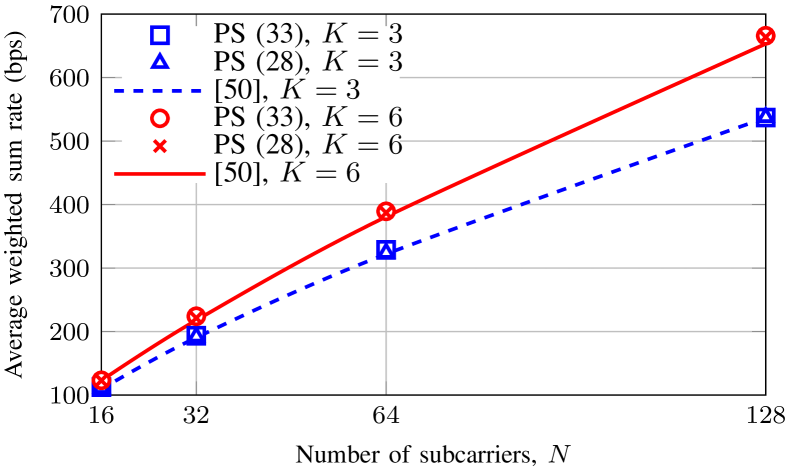
(a) Average weighted sum rate (in bits per second).

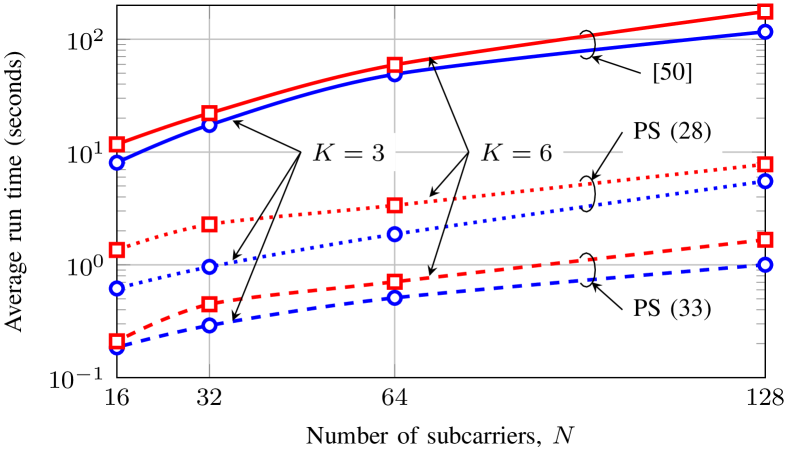
(b) Average run time (in seconds).

Figure 8: Average weighted sum rate and average run time of the proposed solutions (PS (30) and PS (35)) and the solution in [50] for WSRmax problem with different number of subcarrier $N$. The number of transmission links $K$ is taken as 3 and 6.

We first compare the proposed solutions (PS (30) and PS (35)) with the algorithm in [50] for the WSRmax problem. The iterative procedure in [50] stops when the increase in the weighted sum rate of 5 consecutive iterations is less than $10^{-3}.$ The average weighted sum rate performance of the considered methods are plotted in Fig. 8(a) for different numbers of $N$ and $K$. As can be seen, these approaches achieve nearly the same performance in all cases of $K$ and $N$. The complexity comparison of the methods is shown in Fig. 8(b). Clearly, the run time of the GP-based method in [50] scales very fast with $N$, compared to that of the SOCP-based methods. Thus, the GP-based method requires prohibitively high computation time for large $N$. In particular, when $(K,N)=(3,128)$, the proposed solutions (30) and (35) are approximately 20 times and 100 times faster than the method in [50], respectively. Another expected result is that the proposed solution (35) achieves better computational efficiency compared to the proposed solution (30). This gain comes from the facts that the number of variables in (30) is larger than that of (35), and (35) is a QP.

VII-C2 Max-min Fairness Energy Efficiency

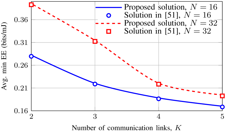
(a) Average minimum energy efficiency (in bits/mJ).

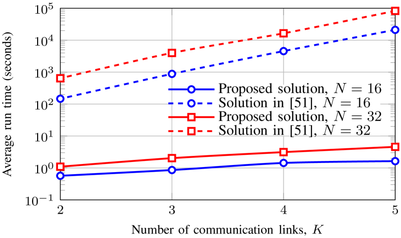
(b) Average run time (in seconds).

Figure 9: Average minimum energy efficiency and average run time of the proposed solution and the solution in [51] for maxminEEfair problem with different sets of $(K,N)$. The circuit power $p_{k}^{\mathrm{c}}$ is $5$ dBm for all $k$.

For maxminEEfair problem, we compare the proposed solution with the two-stage iterative method in [51]. For a fair comparison, the stopping criterion of the two-stage iterative algorithm is as follows. The tolerance error of the inner-stage (i.e. Dinkelbach’s procedure) is $10^{-3}$, and the outer-stage (i.e. the SCA loop) stops when the increase of 5 consecutive iterations is less than $10^{-3}.$ The solver for each subproblem of the two-stage iterative algorithm is FMINCON, which is the general nonlinear solver included in MATLAB’s Optimization Toolbox.

The achieved minimum energy efficiency of the two methods in comparison is shown in Fig. 9(a). In all cases of $(K,N)$, the energy efficiency performance of the two approaches is the same, but there is a huge difference in terms of computation time as shown in Fig. 9(b). Again, we can see that the run time of the proposed solution is much less sensitive to the dimension of the problems, compared to the existing method. In particular, the proposed solution is about $10^{4}$ times faster than the method in [51] for $K=5$ and $N=32$.

VIII Conclusion and Discussion

We have proposed several conic quadratic approximations for wireless communications designs in the context of the SCA paradigm and applied these to solve various design problems, including AF beamforming, cognitive multicasting, MIMO relaying, and multicarrier power controlling. For some specific problems, modifications and customization have been made to improve the solution efficiency. Numerical results have shown that the proposed approximations are far superior to the existing methods in terms of solution speed, while still achieve the same design objective.

For future work, it is interesting to investigate the global optimality of the computed solutions of different approximations proposed in this paper. Another research direction can be finding a flexible and efficient way to switch between different approximations during the iterative process to speed up the convergence.

References

- [1] Cisco White Paper, “Cisco visual networking index: Global mobile data traffic forecast update 2014 - 2019 white paper,” Feb. 2015.
- [2] Samsung White Paper, “5G vision,” Feb. 2015.
- [3] DOCOMO White Paper, “5G radio access: requirements, concept and technologies,” July 2014.
- [4] Z.-Q. Luo and W. Yu, “An introduction to convex optimization for communications and signal processing,” IEEE J. Sel. Areas Commun., vol. 24, no. 8, pp. 1426–1438, Aug 2006.
- [5] A. B. Gershman, N. D. Sidiropoulos, S. Shahbazpanahi, M. Bengtsson, and B. Ottersten, “Convex optimization-based beamforming,” IEEE Signal Process. Mag., vol. 27, no. 3, pp. 62–75, May 2010.
- [6] D. P. Palomar, J. M. Cioffi, and M. A. Lagunas, “Joint Tx-Rx beamforming design for multicarrier MIMO channels: a unified framework for convex optimization,” IEEE Trans. Signal Process., vol. 51, no. 9, pp. 2381–2401, Sept 2003.
- [7] E. Björnson, E. Jorswieck, M. Debbah, and B. Ottersten, “Multiobjective signal processing optimization: The way to balance conflicting metrics in 5G systems,” IEEE Signal Process. Mag., vol. 31, no. 6, pp. 14–23, Nov. 2014.
- [8] Z.-Q. Luo, W.-K. Ma, A. M.-C. So, Y. Ye, and S. Zhang, “Semidefinite relaxation of quadratic optimization problems,” IEEE Signal Process. Mag., vol. 27, no. 3, pp. 20–34, May 2010.
- [9] D. P. Palomar and M. Chiang, “A tutorial on decomposition methods for network utility maximization,” IEEE J. Sel. Areas Commun., vol. 24, no. 8, pp. 1439–1451, Aug. 2006.
- [10] J. F. C. Mota, J. M. F. Xavier, P. M. Q. Aguiar, and M. Püschel, “D-ADMM: A communication-efficient distributed algorithm for separable optimization,” IEEE Trans. Signal Process., vol. 61, no. 10, pp. 2718–2723, May 2013.
- [11] A. Pascual-Iserte, D. P. Palomar, A. I. Perez-Neira, and M. A. Lagunas, “A robust maximin approach for MIMO communications with imperfect channel state information based on convex optimization,” IEEE Trans. Signal Process., vol. 54, no. 1, pp. 346–360, Jan. 2006.
- [12] A. Wiesel, Y. Eldar, and S. Shamai, “Linear precoding via conic optimization for fixed MIMO receivers,” IEEE Trans. Signal Process., vol. 54, no. 1, pp. 161–176, Jan. 2006.
- [13] Z.-Q. Luo and S. Zhang, “Dynamic spectrum management: Complexity and duality,” IEEE J. Sel. Topics Signal Process., vol. 2, no. 1, pp. 57–73, Feb. 2008.
- [14] S. Joshi, P. Weeraddana, M. Codreanu, and M. Latva-aho, “Weighted sum-rate maximization for MISO downlink cellular networks via branch and bound,” IEEE Trans. Signal Process., vol. 60, no. 4, pp. 2090–2095, April 2012.
- [15] O. Tervo, L.-N. Tran, and M. Juntti, “Optimal energy-efficient transmit beamforming for multi-user MISO downlink,” IEEE Trans. Signal Process., vol. 63, no. 20, pp. 5574–5588, Oct. 2015.
- [16] D. Nguyen, L.-N. Tran, P. Pirinen, and M. Latva-aho, “On the spectral efficiency of full-duplex small cell wireless systems,” IEEE Trans. Wireless Commun., vol. 13, no. 9, pp. 4896–4910, Sept. 2014.
- [17] C. Sun, E. A. Jorswieck, and Y. x. Yuan, “Sum rate maximization for non-regenerative MIMO relay networks,” IEEE Trans. Signal Process., vol. 64, no. 24, pp. 6392–6405, Dec. 2016.
- [18] L.-N. Tran, M. Hanif, A. Tolli, and M. Juntti, “Fast converging algorithm for weighted sum rate maximization in multicell MISO downlink,” IEEE Signal Process. Lett., vol. 19, no. 12, pp. 872–875, Dec. 2012.
- [19] O. Mehanna, K. Huang, B. Gopalakrishnan, A. Konar, and N. Sidiropoulos, “Feasible point pursuit and successive approximation of non-convex QCQPs,” IEEE Signal Process. Lett., vol. 22, no. 7, pp. 804–808, July 2015.
- [20] G. Scutari, F. Facchinei, L. Lampariello, S. Sardellitti, and P. Song, “Parallel and distributed methods for constrained nonconvex optimization-part II: Applications in communications and machine learning,” IEEE Trans. Signal Process., vol. 65, no. 8, pp. 1945–1960, April 2017.
- [21] A. H. Phan, H. D. Tuan, H. H. Kha, and D. T. Ngo, “Nonsmooth optimization for efficient beamforming in cognitive radio multicast transmission,” IEEE Trans. Signal Process., vol. 60, no. 6, pp. 2941–2951, June 2012.
- [22] L.-N. Tran, M. Hanif, and M. Juntti, “A conic quadratic programming approach to physical layer multicasting for large-scale antenna arrays,” IEEE Signal Process. Lett., vol. 21, no. 1, pp. 114–117, Jan. 2014.
- [23] B. R. Marks and G. P. Wright, “A general inner approximation algorithm for nonconvex mathematical programs,” Operations Research, vol. 26, no. 4, pp. 681–683, August 1978.
- [24] A. L. Yuille and A. Rangarajan, “The concave-convex procedure,” Neural Computation, vol. 15, no. 4, pp. 915–936, April 2003.
- [25] D. Hunter and K. Lange, “A tutorial on MM algorithms,” Amer. Statistician, vol. 58, pp. 30–37, 2004.
- [26] T. V. Do, H. A. L. Thi, and N. T. Nguyen, Advanced Computational Methods for Knowledge Engineering. Springer, 2014.
- [27] A. Beck, A. Ben-Tal, and L. Tetruashvili, “A sequential parametric convex approximation method with applications to nonconvex truss topology design problems,” Journal of Global Optimization, vol. 47, no. 1, pp. 29–51, 2010.
- [28] G. Scutari, F. Facchinei, and L. Lampariello, “Parallel and distributed methods for constrained nonconvex optimization-part I: Theory,” IEEE Trans. Signal Process., vol. 65, no. 8, pp. 1929–1944, April 2017.
- [29] A. Ben-Tal and A. Nemirovski, Lectures on Modern Convex Optimization. Soc. Ind. Appl. Math. (SIAM), 2001.
- [30] F. Alizadeh and D. Goldfarb, “Second-order cone programming,” Mathematical Programming, vol. 95, pp. 3–51, Jan. 2003.
- [31] M. Lobo, L. Vandenberghe, S. Boyd, and H. Lebret, “Applications of second-order cone programming,” Linear Algebra Appl., pp. 193–228, Nov. 1998.
- [32] Y. Sun, P. Babu, and D. P. Palomar, “Majorization-minimization algorithms in signal processing, communications, and machine learning,” IEEE Trans. Signal Process., vol. 65, no. 3, pp. 794–816, Feb. 2017.
- [33] M. Razaviyayn, M. Hong, and Z.-Q. Luo, “A Unified Convergence Analysis of Block Successive Minimization Methods for Nonsmooth Optimization,” SIAM J. Optim., vol. 23, no. 2, pp. 1126–1153, Jan. 2013.
- [34] J.-S. Pang, M. Razaviyayn, and A. Alvarado, “Computing B-Stationary Points of Nonsmooth DC Programs,” Math. Oper. Res., vol. 42, no. 1, pp. 95–118, Jan 2017.
- [35] T. Dinh Quoc and M. Diehl, “Sequential Convex Programming Methods for Solving Nonlinear Optimization Problems with DC constraints,” ArXiv e-prints, Jul. 2011.
- [36] Q.-D. Vu, L.-N. Tran, R. Farrell, and E.-K. Hong, “An efficiency maximization design for SWIPT,” IEEE Signal Process. Lett., vol. 22, no. 12, pp. 2189–2193, Dec. 2015.
- [37] T. Lipp and S. Boyd, “Variations and extension of the convex–concave procedure,” Optimization and Engineering, vol. 17, no. 2, pp. 263–287, 2016.
- [38] T. P. Dinh and H. A. L. Thi, “Recent advances in DC programming and DCA,” Transactions on Computational Intelligence XIII, vol. 8342, pp. 1–37, April 2014.
- [39] A. Alvarado, G. Scutari, and J.-S. Pang, “A new decomposition method for multiuser DC-programming and its applications,” IEEE Trans. Signal Process., vol. 62, no. 11, pp. 2984–2998, June 2014.
- [40] M. Razaviyayn, Successive Convex Approximation: Analysis and Applications. University of Minnesota Digital Conservancy, 2014.
- [41] H. Kha, H. Tuan, and H. Nguyen, “Fast global optimal power allocation in wireless networks by local D.C. programming,” IEEE Trans. Wireless Commun., vol. 11, no. 2, pp. 510–515, Feb 2012.
- [42] Y. Li, M. Sheng, X. Wang, Y. Zhang, and J. Wen, “Max-min energy-efficient power allocation in interference-limited wireless networks,” IEEE Trans. Veh. Technol., vol. 64, no. 9, pp. 4321–4326, Sept 2015.
- [43] M. Chiang, C. W. Tan, D. P. Palomar, D. O’Neill, and D. Julian, “Power control by geometric programming,” IEEE Trans. Wireless Commun., vol. 6, pp. 2640–2651, July 2007.
- [44] J. Löfberg, “YALMIP : A toolbox for modeling and optimization in MATLAB,” in Proc. the CACSD Conference, Taipei, Taiwan., 2004.
- [45] I. MOSEK ApS, 2014, [Online]. Available: www.mosek.com.
- [46] Y. Yang, Q. Li, W.-K. Ma, J. Ge, and P. Ching, “Cooperative secure beamforming for AF relay networks with multiple eavesdroppers,” IEEE Signal Process. Lett., vol. 20, no. 1, pp. 35–38, Jan 2013.
- [47] N. Sidiropoulos, T. Davidson, and Z.-Q. Luo, “Transmit beamforming for physical-layer multicasting,” IEEE Trans. Signal Process., vol. 54, no. 6, pp. 2239–2251, June 2006.
- [48] E. Karipidis, N. Sidiropoulos, and Z.-Q. Luo, “Quality of service and max-min fair transmit beamforming to multiple cochannel multicast groups,” IEEE Trans. Signal Process., vol. 56, no. 3, pp. 1268–1279, March 2008.
- [49] A. Phan, H. Tuan, H. Kha, and H. Nguyen, “Iterative D.C. optimization of precoding in wireless MIMO relaying,” IEEE Trans. Wireless Commun., vol. 12, no. 4, pp. 1617–1627, April 2013.
- [50] T. Wang and L. Vandendorpe, “On the SCALE algorithm for multiuser multicarrier power spectrum management,” IEEE Trans. Signal Process., vol. 60, no. 9, pp. 4992–4998, Sept 2012.
- [51] A. Zappone, L. Sanguinetti, G. Bacci, E. Jorswieck, and M. Debbah, “Energy-efficient power control: A look at 5G wireless technologies,” IEEE Trans. Signal Process., vol. 64, no. 7, pp. 1668–1683, April 2016.
- [52] J. Papandriopoulos and J. S. Evans, “SCALE: A low-complexity distributed protocol for spectrum balancing in multiuser DSL networks,” IEEE Trans. Inf. Theory, vol. 55, no. 8, pp. 3711–3724, Aug 2009.