Radiative lifetimes of dipolar excitons in double quantum-wells

Abstract

Spatially indirect excitons in semiconducting double quantum wells have been shown to exhibit rich collective many-body behavior that result from the nature of the extended dipole-dipole interactions between particles. For many spectroscopic studies of the emission from a system of such indirect excitons, it is crucial to separate the single particle properties of the excitons from the many-body effects arising from their mutual interactions. In particular, knowledge of the relation between the emission energy of indirect excitons and their radiative lifetime could be highly beneficial for control, manipulation, and analysis of such systems. Here we study a simple analytic approximate relation between the radiative lifetime of indirect excitons and their emission energy. We show, both numerically and experimentally, the validity and the limits of this approximate relation. This relation between the emission energy and the lifetime of indirect excitons can be used to tune and determine their lifetime and their resulting dynamics without the need of directly measuring it, and as a tool for design of indirect exciton based devices.

I Introduction

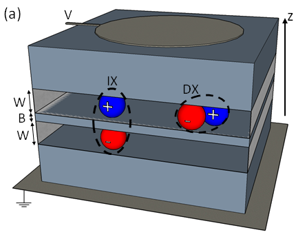
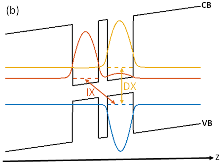
Figure 1: (a) A simplified illustration of the typical realization of IXs in semiconductor DQW heterostructure. Two quantum wells of width $W$ are separated by a thin central barrier layer marked as $B$. A metallic gate is positioned on the top of the sample, allowing the induction of electric field in the $z$ direction. Bound pairs of $e$ (red sphere) and $h$ (blue sphere) are created in the wells by optical excitation and can occupy the DX state - where both particles reside in the same well, or in the IX state - where each of them resides in a different well. (b) A typical energy diagram, illustrating the conduction (CB) and valence (VB) energy bands along the $z$ axis, the wavefunctions of the $h$ (blue line) and the $e$ occupying the DX (yellow line) and IX (red line) states, and their corresponding energies (dashed lines). The external electric field is responsible to the tilt of the energy bands, making the IX state lower in energy than the DX state.

An indirect exciton (IX) is a coulomb-bound complex of an electron ($e$) and a hole ($h$) where the opposite charges of the bound complex are spatially separated in two parallel layers with a tunneling barrier between them, as is depicted in Fig. 1. Such IXs are usually formed by optical excitation of an electrically biased double quantum well (DQW) heterostructure rapaport_experimental_2007 ; butov_condensation_2004 ; butov_cold_2007 . This spatial $e$-$h$ separation leads to a long radiative lifetime and to a large electrical dipole moment of the IX. Due to the combination of these two properties, IXs give a unique opportunity to observe and study interesting cold interacting low-dimensional fluids. In recent years, an intensive experimental and theoretical effort focused on IX fluids in GaAs based DQWs revealed many intriguing many-body phenomena, such as spontaneous pattern formation butov_macroscopically_2002 ; snoke_long-range_2002 ; rapaport_charge_2004 ; butov_formation_2004 , spin textures high_spin_2013 , interaction-induced particle correlations laikhtman_exciton_2009 ; shilo_particle_2013 , molecular IX complexes schinner_confinement_2013 ; cohen_vertically_2016 , as well as evidence for complex collective phases butov_towards_2002 ; combescot_bose-einstein_2007 ; shilo_particle_2013 ; alloing_evidence_2014 ; stern_exciton_2014 ; cohen_dark_2016 . On the other hand, recent progress in the techniques for control and manipulation of IXs led to demonstration of various kinds of complex device functionalities such as trapping schemes rapaport_electrostatic_2005 ; hammack_trapping_2006 ; kowalik-seidl_tunable_2012 ; schinner_confinement_2013 ; alloing_optically_2013 ; schinner_confinement_2013 , flow control, IX transport and routing high_control_2008 ; violante_dynamics_2014 ; winbow_electrostatic_2011 ; cohen_remote_2011 ; lazic_scalable_2014 ; violante_dynamics_2014 , and spin transport leonard_spin_2009 ; kowalik-seidl_long_2010 .

Due to these recent advancements, cold IX fluids started attracting the interest of a wider scientific community, and new experiments on dipolar fluids of IXs in newly emerging systems have been performed recently. These include bilayer two-dimensional transition metal DiChalcagonide systems rivera_observation_2015 , bilayer graphene li_negative_2016 ; li_excitonic_2016 and polaritonic systems cristofolini_coupling_2012 ; rosenberg_electrically_2016 among others.

To fully understand and control the various properties of such optically generated IX fluids, it is very important to have a good insight on their intrinsic dynamics. A key property of the IX dynamics is the radiative lifetime. This radiative lifetime due to the $e$-$h$ optical recombination is the dominant loss process in such systems, and can in principle be measured directly by time-resolved measurement of the decay of their photoluminescence after a pulse excitation phillips_theoretical_1989 ; golub_long-lived_1990 ; alexandrou_electric-field_1990 ; charbonneau_transformation_1988 . However, as many experiments are done in a steady state under continuous-wave excitation and do not involve a direct lifetime measurement, a method of inferring the lifetime from other measurable quantities can be very useful. In particular, when designing a sample, a complex device, or an experiment, a prior knowledge and understanding of such recombination dynamics could be essential. Previous theoretical works have proposed various general approaches allowing numerical calculation of the IX’s lifetime galbraith_exciton_1989 ; kamizato_excitons_1989 ; lee_excitonic_1989 ; dignam_exciton_1991 ; linnerud_exciton_1994 ; takahashi_effect_1994 ; soubusta_excitonic_1999 ; szymanska_excitonic_2003 ; arapan_exciton_2005 ; sivalertporn_direct_2012 . In our previous work shilo_particle_2013 we have presented a simple approximated analytic model according to which the radiative lifetime of an IX is simply related to its emission energy. This model allows inferring relative radiative lifetimes of IXs within a limited range of experimental conditions, from their corresponding eigen-energies, without the need for complex numerical calculations. These eigen-enegies could in turn be easily measured - for example, from the emission spectra - or be calculated numerically using rather simple computer solvers.

In the model of Ref. shilo_particle_2013, the recombination lifetime of an IX is inversely proportional to the squared overlap integral between the envelop wavefunctions of the $e$ and the $h$:

$$\tau_{id}=\frac{\tau_{d}}{\left|\braket{\psi_{e}}{\psi_{h}}\right|^{2}}$$ (1)

where $\tau_{id}$, $\tau_{d}$ are the lifetimes of the IX and of the direct exciton (DX), respectively and $\psi_{e}$, $\psi_{h}$ are the envelop wavefunctions of the $e$ and the $h$ along the DQW growth ($z$) direction, respectively. Fig.  1 schematically illustrates both the DX and IX states in a DQW under an applied electric field along the $z$-axis.

Under a weak enough external electric field, the lowest energy $e$ and $h$ envelope wavefunctions can be approximated as a linear combination of the corresponding lowest energy flat-band SQW wavefunctions bastard_wave_1988 :

$$\psi^{e}(z) =c^{e}_{l}\psi^{e}_{l}(z)+c^{e}_{r}\psi^{e}_{r}(z)$$ (2)

$$\psi^{h}(z) =c^{h}_{l}\psi^{h}_{l}(z)+c^{h}_{r}\psi^{h}_{r}(z).$$ (3)

Initially, increasing the field will only effect the coefficients and not the validity of the approximation itself. However, when the field becomes strong enough such that the potential drop across each QW is of the order of the difference between the ground energy in the SQW and its first excited state energy, this approximation breaks. Such strong field leads to a substantial admixture of excited states, shifting the peak of the wavefunction away from the center of the corresponding QW. Another approximation can be made in cases where the effective mass of the $h$ is significantly larger than the effective mass of the $e$, and under a large enough external field. Under such circumstances, the lowest energy $h$’s wavefunction can be well approximated by only one SQW wavefunction, i.e., $\psi^{h}(z)=\psi^{h}_{r}(z)$ in the case of an electric field applied in the positive $z$-direction, as is illustrated in Fig. 1b. As a result, if the external field is strong enough, the computation of the overlap integral $\braket{\psi_{e}}{\psi_{h}}$ of Eq. 1 can be approximated by integration of the $e$’s wavefunction only inside the right QW in which the $h$’s wavefunction is strongly confined. Thus, there is an intermediate range of electric field values in which both of the above approximations should hold to a good accuracy. Within this range, the computation of the recombination lifetime is reduced to the computation of $c^{e}_{r}$ - the amplitude of the $e$’s wavefunction in the $h$’s well:

$$\tau_{id}=\frac{\tau_{d}}{|c_{r}^{e}|^{2}}$$ (4)

As was shown in Ref. shilo_particle_2013, , diagonalizing the Hamiltonian for the electron in the basis of $\psi_{l}^{e}$ and $\psi_{r}^{e}$, yields:

$$c_{r}^{e}=\frac{t}{E_{d}-E_{id}}$$ (5)

where $E_{d}$ and $E_{id}$ are the energies of the DX and IX respectively and $t$ is the following tunnelling matrix element:

$$t=\braket{\psi_{l}^{e}}{(T+V_{e}(z))}{\psi_{r}^{e}}-\braket{\psi_{l}^{e}}{\psi_{r}^{e}}E_{0}$$ (6)

with $T$ the kinetic energy, $V_{e}(z)$ is the electron’s DQW potential, and $E_{0}$ the ground state energy of a non-interacting electron in a SQW potential. The expression in Eq.  5 was obtained under the assumption that all other contributions to the potential energy (i.e., the external electric field, the interaction of the electron with neighboring IXs and its coulomb interaction with the $h$) contribute only negligible corrections to $t$. Additionally, it assumes that the tunneling matrix element $t$ is small compared to the energy difference between the DX and the IX, i.e.

$$t\ll\frac{1}{2}(E_{d}-E_{id}).$$ (7)

Under the limitations and assumptions mentioned above, the radiative lifetime of an IX can approximately be expressed as shilo_particle_2013 :

$$\frac{1}{\tau_{id}}=\frac{1}{\tau_{d}}\frac{t^{2}}{\left(E_{d}-E_{id}\right)^{2}}.$$ (8)

In this work we numerically test the accuracy and validity limits of Eq.  8 and provide an experimental confirmation that it holds to a good accuracy in the expected validity range.

The structure of this paper is as follows: in Sec.  II we compare that analytic result to a numerical calculation using a coupled Schrödinger-Poisson solver under a mean-field approximation of the interactions between IXs. In Sec.  III we present experimental results confirming the validity of Eq.  8 and of the underlying approximations. In Sec.  IV we summarize our results and their conclusions.

II Comparison to numerical calculations

To check the validity, accuracy, and applicability limits of Eq.  8, we first compared its predictions with numerical calculations of the overlap between the envelop wavefunctions of the $e$ and the $h$, using a one-dimensional, self-consistent, Schrödinger-Poisson solver harrison_quantum_2000 . In the numerical model, we assumed a mean-field approximation for the IX-IX interactions, where in-plane dipolar correlationslaikhtman_exciton_2009 were neglected, as well as the binding interaction between the $e$ and the $h$. For any given applied field $F$ and IX density $n$, we obtained from the solver the $e$ and $h$ envelope wavefunctions and numerically computed their overlap integral. The IX radiative lifetime is inversely proportional to the square of this overlap integral, and thus it can be calculated up to a multiplicative constant. More importantly, the ratio between the lifetime of the DX and the IX can also be calculated in this way as:

$$\frac{\tau_{d}}{\tau_{id}}=\frac{\left|\braket{\psi_{e}^{(1)}}{\psi_{h}^{(1)}}\right|^{2}}{\left|\braket{\psi_{e}^{(2)}}{\psi_{h}^{(1)}}\right|^{2}}$$ (9)

where the superscripts mark the corresponding quantum number of the $e$ and $h$ energy levels in the DQW. Substituting into Eq. 8 we get the following equation:

$$\frac{\left|\braket{\psi_{e}^{(1)}}{\psi_{h}^{(1)}}\right|^{2}}{\left|\braket{\psi_{e}^{(1)}}{\psi_{h}^{(2)}}\right|^{2}}=\frac{t^{2}}{\left(E_{d}-E_{id}\right)^{2}}.$$ (10)

Since the same numerical solver also yields $E_{d}-E_{id}$, the accuracy of this equality can be used to check the accuracy of Eq.  8, after plugging in the transition matrix element $t$.

The transition matrix element $t$ can be approximated numerically using the SQW wavefunctions $\psi_{r}$ and $\psi_{l}$, according to Eq.  6. We carried this calculation for a semi-infinite narrow DQW structure having a $4nm$-wide central barrier, and for different realistic GaAs DQW structures, all having $\ce{Al_{0.5}Ga_{0.5}As}$ barriers and $4nm$-wide central barriers. The GaAs QWs have widths of $8nm$, $10nm$, $12nm$ and $14nm$, respectively. The values of $t$ for these four GaAs DQWs are $0.36meV$, $0.2meV$, $0.13meV$, and $0.09meV$ respectively.

The relative error $\Delta$ of Eq.  10 is defined as $(r.h.s-l.h.s)/l.h.s$, i.e.

$$\Delta\equiv\frac{t^{2}}{\left(E_{d}-E_{id}\right)^{2}}\times\frac{\left|\braket{\psi_{e}^{(1)}}{\psi_{h}^{(2)}}\right|^{2}}{\left|\braket{\psi_{e}^{(1)}}{\psi_{h}^{(1)}}\right|^{2}}-1.$$ (11)

This error is computed and presented in Fig.  2a as a function of $E_{d}-E_{id}$ for four different DQW structures differing by their well widths, for the single-IX case (i.e. where the IX-IX interaction is set to zero). Here the values of $E_{d}-E_{id}$ are determined solely by $F$. The dependence of the relative error $\Delta$ on $E_{d}-E_{id}$ is in agreement with the expected limits of validity mentioned in the previous section: where $E_{d}-E_{id}$ is very small, the penetration of the $h$’s wavefunction into the $e$’s QW is significant and Eq. 8 over-estimates the radiative lifetime. Once the field is increased such that $E_{d}-E_{id}$ becomes larger than $t$, the error drops rapidly and stays low for quite a wide range of $E_{d}-E_{id}$ values. At even larger values of $E_{d}-E_{id}$, both the $e$’s and the $h$’s wavefunctions distort in opposite directions and their overlap integral is further diminished. The analytic model does not take this distortion into account (as each of the basis wavefunctions used $\psi_{l}$ and $\psi_{r}$ is of a flat bottom QW), and so it underestimates the lifetime, resulting in a relative error which grows with $E_{d}-E_{id}$ in the negative direction. As expected, this distortion increases with the width of the QWs, leading to a wider $E_{d}-E_{id}$ range having a high relative accuracy of Eq. 8 for narrower DQWs.

We note that this calculation neglect the $e-h$ coulomb attraction, which tends to reduce the above distortion of the single particle wavefunctions with increasing $F$. In this sense the error values presented in in Fig.  2a are an overestimate of the expected error of Eq. 8.

Fig.  2b presents the relative error as a function of the IX density $n$, for a fixed value $E_{d}-E_{id}=5$ meV. This is done by setting different values of $n$ and finding the corresponding values of $F$ to keep $E_{d}-E_{id}$ constant (this method, named ’constant energy line method’, was extensively used in our previous experimental works shilo_particle_2013 ; cohen_dark_2016 ). As seen in the figure, the relatively low error values are maintained up to a high IX density of $n\simeq 10^{11}$cm^-2. Above this value, the inhomogeneous distribution of the IX charge density along the z-axis of the QWs is large enough to induce large deviations of the $e$ and $h$ wavefunctions from the single particle wavefunctions, leading to a decrease in the accuracy of Eq.  8.

These numerical calculations demonstrate that Eq. 8 is a good approximation over a significant range of applied electric fields and IX densities and can be tested in experiments, as we show in the next section.

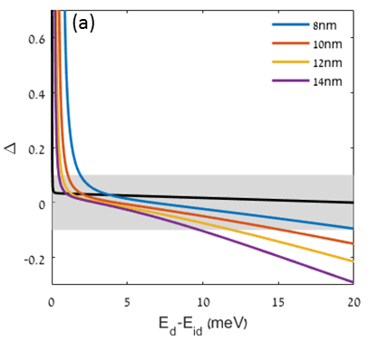
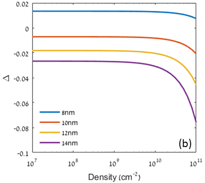
Figure 2: (a) The relative error $\Delta$ of Eq.  10, defined in Eq.  11, plotted against $E_{d}-E_{id}$ for four different widths (different W’s) of a GaAs/$\ce{Al_{0.5}Ga_{0.5}As}$ DQW. The shaded area marks the region where $|\Delta|<0.1$ and the black curve is $\Delta$ calculated for the limit of a quasi-infinite, narrow DQW structure, also having a $4$nm-wide central barrier. (b) $\Delta$ as a function of the IX density $n$ while the external field is adjusted to keep the constant value of $E_{d}-E_{id}=5$ meV, for each of the four DQW structures.

III Comparison to experiments

III.1 Experimental details

The experimental scheme is rather similar to that presented in few of our previous works shilo_particle_2013 ; cohen_dark_2016 . The sample, positioned in an optical $\ce{{}^{4}He}$ cryostat, is a $12/4/12$nm $GaAs/Al_{0.5}Ga_{0.5}As/GaAs$ DQW structure grown on an $n^{+}$-doped GaAs substrate and with a $10$nm-thick, semi-transparent Ti electrode positioned on its top cohen_dark_2016 . The overall thickness of the sample is about $3\mu m$. An electric field between the top electrode and the doped substrate creates the energy band tilt required for the formation of IXs and allows their trapping as presented in fig  3a-b. The sample temperature is maintained at $T=1.8$K.

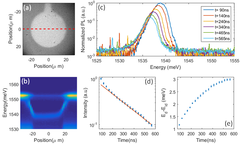
Figure 3: (a) A real-space image of the circular electrostatic trap used in this work. (b) A spectral-spatial image of the emission from the sample as a function of the position of a CW laser excitation along the dashed red line drawn in (a), with a reversed voltage set to $1V$, an excitation power of $1500$nW and temperature of $1.8K$. The trapping potential is flat around the center of the trap with $E_{d}-E_{id}\simeq 12$meV. (c) Exemplary time resolved and spatially integrated spectra at different times after the laser excitation. (d) Integrated intensity $I$ and (e) $(E_{d}-E_{id})$ as a function of time after the laser pulse extracted from the data in (c). All time frames are integrated over a $25$ns-wide window.

A population of IXs is being excited using a non-resonant pulsed laser having wavelength of $775nm$ and pulse duration of $300ps$, under a fixed applied electric bias. We then study the decay of the population after the pulse excitation, by time-resolved measurement of the light emitted by recombination of the optically active (i.e ’bright’) IXs, using a fast-gated ICCD camera (Princeton Instruments PIMAX).

III.2 Results

Exemplary time resolved, spatially integrated spectra at different times after the laser excitation are presented in Fig.  3c, for a fixed applied bias of 1V. The spectral lines have a tail to the long wavelength side, similarly to previous results. Fig.  3d,e present the integrated intensity and the IX energy as a function of time after the excitation. The observed redshift during the decay results from the decrease of the interaction energy as the IX density decreases shilo_particle_2013 .

The radiative recombination of IXs can be described by a simple rate equation:

$$I(t)\propto\frac{\partial n}{\partial t}=\frac{n(t)}{\tau_{id}(t)}$$ (12)

where $I$ is the measured emission intensity. Using $n(t)\propto\int_{t}^{\infty}I(t^{\prime})dt^{\prime}$, and expressing $\tau_{id}(t)$ using Eq. 8 the following relation is obtained:

$$I(t)\propto\frac{\int_{t}^{\infty}I(t^{\prime})dt^{\prime}}{\left(E_{d}-E_{id}(t)\right)^{2}}\equiv G(t)$$ (13)

and both $I(t)$ and $G(t)$ can be directly expressed for every $t$ from the experimental results in Fig.  3d,e. The assumptions made in this last derivation are the accuracy of Eq.  8 and that the recombination process is radiatively dominated. Thus, if these assumptions are valid we expect that Eq. 13 should hold for our experimental results, i.e., we expect to find that $G(t)\propto I(t)$ for every $t$ along the whole decay. This is therefore a direct experimental test for Eq.  8.

Fig.  4 presents the experimentally extracted $G(t)$ versus $I(t)$ for four different decay traces that were measured under fixed lattice temperature of $1.8K$ ($\pm 0.1K$) and different external applied biases and laser powers. The solid lines are linear fits to the data. A clear linear dependence is observed, confirming the validity of the above assumptions and thus the accuracy of Eq.  8 for this range of experimental parameters.

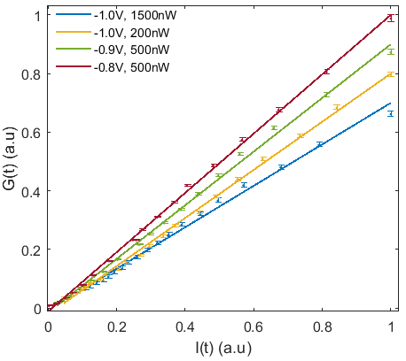
Figure 4: Experimentally extracted $G(t)$ versus $I(t)$ for four different decay traces that were measured under fixed lattice temperature of $1.8K$ ($\pm 0.1K$) and different external applied biases and laser powers. The solid lines are linear fits to the data. A clear linear dependence is observed, confirming the validity of Eq.  8 for this range of experimental parameters (The temporal dynamics in each of these measurements is from top-right to bottom-left).

IV Conclusion

In this work we presented a numerical and experimental test of an approximated derivation relating the IX radiative lifetime to its energy. We showed that this relation holds well for a wide range of accessible experimental parameters and thus also confirmed our assumptions used in our previous works shilo_particle_2013 ; cohen_dark_2016 . We conclude that this relation can be very useful for future works studying IXs in similar bilayer systems, simplifying the analysis of dynamics of IX systems. In many such experiments, the lifetime is a key property whose assessment is not a straight-forward task under the required experimental settings. This difficulty could be relieved by the proposed method, which in principle requires a single calibration measurement to set right the proportion coefficient of Eq.  8 for the sample of interest.

As demonstrated above by the numerical simulation, Eq.  8 is only valid and accurate enough in an intermediate range of IX energies: the basic picture described by the theoretical model becomes valid only when the separation between the energies of the indirect and the direct excitons is large enough. As the separation is increase further, the accuracy of the model gradually deteriorate and the error of Eq.  8 grows. Between these two ends, lies the range of IX energies where the error is relatively low and Eq.  8 can be used as a good approximation.

We believe that this method can be easily modified for other IX structures that are currently being explored, such as IXs in bilayers of other material systems.

- (1) R. Rapaport and G. Chen, “Experimental methods and analysis of cold and dense dipolar exciton fluids,” Journal of Physics: Condensed Matter, vol. 19, no. 29, p. 295207, 2007.
- (2) L. V. Butov, “Condensation and pattern formation in cold exciton gases in coupled quantum wells,” Journal of Physics: Condensed Matter, vol. 16, no. 50, p. R1577, 2004.
- (3) L. V. Butov, “Cold exciton gases in coupled quantum well structures,” Journal of Physics: Condensed Matter, vol. 19, no. 29, p. 295202, 2007.
- (4) L. V. Butov, A. C. Gossard, and D. S. Chemla, “Macroscopically ordered state in an exciton system,” Nature, vol. 418, pp. 751–754, Aug. 2002.
- (5) D. Snoke, S. Denev, Y. Liu, L. Pfeiffer, and K. West, “Long-range transport in excitonic dark states in coupled quantum wells,” Nature, vol. 418, pp. 754–757, Aug. 2002.
- (6) R. Rapaport, G. Chen, D. Snoke, S. H. Simon, L. Pfeiffer, K. West, Y. Liu, and S. Denev, “Charge Separation of Dense Two-Dimensional Electron-Hole Gases: Mechanism for Exciton Ring Pattern Formation,” Physical Review Letters, vol. 92, p. 117405, Mar. 2004.
- (7) L. V. Butov, L. S. Levitov, A. V. Mintsev, B. D. Simons, A. C. Gossard, and D. S. Chemla, “Formation Mechanism and Low-Temperature Instability of Exciton Rings,” Physical Review Letters, vol. 92, p. 117404, Mar. 2004.
- (8) A. A. High, A. T. Hammack, J. R. Leonard, S. Yang, L. V. Butov, T. Ostatnicky, M. Vladimirova, A. V. Kavokin, T. C. H. Liew, K. L. Campman, and A. C. Gossard, “Spin Currents in a Coherent Exciton Gas,” Physical Review Letters, vol. 110, p. 246403, June 2013.
- (9) B. Laikhtman and R. Rapaport, “Exciton correlations in coupled quantum wells and their luminescence blue shift,” Physical Review B, vol. 80, p. 195313, Nov. 2009.
- (10) Y. Shilo, K. Cohen, B. Laikhtman, K. West, L. Pfeiffer, and R. Rapaport, “Particle correlations and evidence for dark state condensation in a cold dipolar exciton fluid,” Nature Communications, vol. 4, p. 2335, Aug. 2013.
- (11) G. J. Schinner, J. Repp, E. Schubert, A. K. Rai, D. Reuter, A. D. Wieck, A. O. Govorov, A. W. Holleitner, and J. P. Kotthaus, “Confinement and Interaction of Single Indirect Excitons in a Voltage-Controlled Trap Formed Inside Double InGaAs Quantum Wells,” Physical Review Letters, vol. 110, p. 127403, Mar. 2013.
- (12) K. Cohen, M. Khodas, B. Laikhtman, P. V. Santos, and R. Rapaport, “Vertically coupled dipolar exciton molecules,” Physical Review B, vol. 93, p. 235310, June 2016.
- (13) L. V. Butov, C. W. Lai, A. L. Ivanov, A. C. Gossard, and D. S. Chemla, “Towards Bose-Einstein condensation of excitons in potential traps,” Nature, vol. 417, pp. 47–52, May 2002.
- (14) M. Combescot, O. Betbeder-Matibet, and R. Combescot, “Bose-Einstein Condensation in Semiconductors: The Key Role of Dark Excitons,” Physical Review Letters, vol. 99, p. 176403, Oct. 2007.
- (15) M. Alloing, M. Beian, M. Lewenstein, D. Fuster, Y. González, L. González, Combescot, R., M. Combescot, and F. Dubin, “Evidence for a Bose-Einstein condensate of excitons,” EPL (Europhysics Letters), vol. 107, no. 1, p. 10012, 2014.
- (16) M. Stern, V. Umansky, and I. Bar-Joseph, “Exciton Liquid in Coupled Quantum Wells,” Science, vol. 343, pp. 55–57, Jan. 2014.
- (17) K. Cohen, Y. Shilo, K. West, L. Pfeiffer, and R. Rapaport, “Dark High Density Dipolar Liquid of Excitons,” Nano Letters, vol. 16, pp. 3726–3731, June 2016.
- (18) R. Rapaport, G. Chen, S. Simon, O. Mitrofanov, L. Pfeiffer, and P. M. Platzman, “Electrostatic traps for dipolar excitons,” Physical Review B, vol. 72, p. 075428, Aug. 2005.
- (19) A. T. Hammack, M. Griswold, L. V. Butov, L. E. Smallwood, A. L. Ivanov, and A. C. Gossard, “Trapping of Cold Excitons in Quantum Well Structures with Laser Light,” Physical Review Letters, vol. 96, p. 227402, June 2006.
- (20) K. Kowalik-Seidl, X. P. Vögele, B. N. Rimpfl, G. J. Schinner, D. Schuh, W. Wegscheider, A. W. Holleitner, and J. P. Kotthaus, “Tunable Photoemission from an Excitonic Antitrap,” Nano Letters, vol. 12, pp. 326–330, Jan. 2012.
- (21) M. Alloing, A. Lemaître, E. Galopin, and F. Dubin, “Optically programmable excitonic traps,” Scientific Reports, vol. 3, Apr. 2013.
- (22) A. A. High, E. E. Novitskaya, L. V. Butov, M. Hanson, and A. C. Gossard, “Control of Exciton Fluxes in an Excitonic Integrated Circuit,” Science, vol. 321, pp. 229–231, July 2008.
- (23) A. Violante, K. Cohen, S. Lazic, R. Hey, R. Rapaport, and P. V. Santos, “Dynamics of indirect exciton transport by moving acoustic fields,” New Journal of Physics, vol. 16, no. 3, p. 033035, 2014.
- (24) A. G. Winbow, J. R. Leonard, M. Remeika, Y. Y. Kuznetsova, A. A. High, A. T. Hammack, L. V. Butov, J. Wilkes, A. A. Guenther, A. L. Ivanov, M. Hanson, and A. C. Gossard, “Electrostatic Conveyer for Excitons,” Physical Review Letters, vol. 106, p. 196806, May 2011.
- (25) K. Cohen, R. Rapaport, and P. V. Santos, “Remote Dipolar Interactions for Objective Density Calibration and Flow Control of Excitonic Fluids,” Physical Review Letters, vol. 106, p. 126402, Mar. 2011.
- (26) S. Lazic, A. Violante, K. Cohen, R. Hey, R. Rapaport, and P. V. Santos, “Scalable interconnections for remote indirect exciton systems based on acoustic transport,” Physical Review B, vol. 89, p. 085313, Feb. 2014.
- (27) J. R. Leonard, Y. Y. Kuznetsova, S. Yang, L. V. Butov, T. Ostatnický, A. Kavokin, and A. C. Gossard, “Spin Transport of Excitons,” Nano Letters, vol. 9, pp. 4204–4208, Dec. 2009.
- (28) K. Kowalik-Seidl, X. P. Vögele, B. N. Rimpfl, S. Manus, J. P. Kotthaus, D. Schuh, W. Wegscheider, and A. W. Holleitner, “Long exciton spin relaxation in coupled quantum wells,” Applied Physics Letters, vol. 97, p. 011104, July 2010.
- (29) P. Rivera, J. R. Schaibley, A. M. Jones, J. S. Ross, S. Wu, G. Aivazian, P. Klement, K. Seyler, G. Clark, N. J. Ghimire, J. Yan, D. G. Mandrus, W. Yao, and X. Xu, “Observation of long-lived interlayer excitons in monolayer MoSe2-WSe2 heterostructures,” Nature Communications, vol. 6, p. 6242, Feb. 2015.
- (30) J. I. A. Li, T. Taniguchi, K. Watanabe, J. Hone, A. Levchenko, and C. R. Dean, “Negative Coulomb Drag in Double Bilayer Graphene,” Physical Review Letters, vol. 117, p. 046802, July 2016.
- (31) J. I. A. Li, T. Taniguchi, K. Watanabe, J. Hone, and C. R. Dean, “Excitonic superfluid phase in Double Bilayer Graphene,” arXiv:1608.05846 [cond-mat], Aug. 2016. arXiv: 1608.05846.
- (32) P. Cristofolini, G. Christmann, S. I. Tsintzos, G. Deligeorgis, G. Konstantinidis, Z. Hatzopoulos, P. G. Savvidis, and J. J. Baumberg, “Coupling Quantum Tunneling with Cavity Photons,” Science, vol. 336, pp. 704–707, May 2012.
- (33) I. Rosenberg, Y. Mazuz-Harpaz, R. Rapaport, K. West, and L. Pfeiffer, “Electrically controlled mutual interactions of flying waveguide dipolaritons,” Physical Review B, vol. 93, p. 195151, May 2016.
- (34) C. C. Phillips, R. Eccleston, and S. R. Andrews, “Theoretical and experimental picosecond photoluminescence studies of the quantum-confined Stark effect in a strongly coupled double-quantum-well structure,” Physical Review B, vol. 40, pp. 9760–9766, Nov. 1989.
- (35) J. E. Golub, K. Kash, J. P. Harbison, and L. T. Florez, “Long-lived spatially indirect excitons in coupled GaAs/Al x Ga 1− x As quantum wells.,” Physical Review B, vol. 41, pp. 8564–8567, Apr. 1990.
- (36) A. Alexandrou, J. A. Kash, E. E. Mendez, M. Zachau, J. M. Hong, T. Fukuzawa, and Y. Hase, “Electric-field effects on exciton lifetimes in symmetric coupled GaAs/Al 0.3 Ga 0.7 As double quantum wells.,” Physical Review B, vol. 42, pp. 9225–9228, Nov. 1990.
- (37) S. Charbonneau, M. L. W. Thewalt, E. S. Koteles, and B. Elman, “Transformation of spatially direct to spatially indirect excitons in coupled double quantum wells,” Physical Review B, vol. 38, pp. 6287–6290, Sept. 1988.
- (38) I. Galbraith and G. Duggan, “Exciton binding energy and external-field-induced blue shift in double quantum wells,” Physical Review B, vol. 40, pp. 5515–5521, Sept. 1989.
- (39) T. Kamizato and M. Matsuura, “Excitons in double quantum wells,” Physical Review B, vol. 40, pp. 8378–8384, Oct. 1989.
- (40) J. Lee, M. O. Vassell, E. S. Koteles, and B. Elman, “Excitonic spectra of asymmetric, coupled double quantum wells in electric fields,” Physical Review B, vol. 39, pp. 10133–10143, May 1989.
- (41) M. M. Dignam and J. E. Sipe, “Exciton states in coupled double quantum wells in a static electric field,” Physical Review B, vol. 43, pp. 4084–4096, Feb. 1991.
- (42) I. Linnerud and K. A. Chao, “Exciton binding energies and oscillator strengths in a symmetric Al x Ga 1− x As/GaAs double quantum well.,” Physical Review B, vol. 49, pp. 8487–8490, Mar. 1994.
- (43) Y. Takahashi, Y. Kato, S. S. Kano, S. Fukatsu, Y. Shiraki, and R. Ito, “The effect of electric field on the excitonic states in coupled quantum well structures,” Journal of Applied Physics, vol. 76, pp. 2299–2305, Aug. 1994.
- (44) J. Soubusta, R. Grill, P. Hlidek, M. Zvara, L. Smrcka, S. Malzer, W. Geisselbrecht, and G. H. Dohler, “Excitonic photoluminescence in symmetric coupled double quantum wells subject to an external electric field,” Physical Review B, vol. 60, pp. 7740–7743, Sept. 1999.
- (45) M. H. Szymanska and P. B. Littlewood, “Excitonic binding in coupled quantum wells,” Physical Review B, vol. 67, p. 193305, May 2003.
- (46) S. C. Arapan and M. A. Liberman, “Exciton levels and optical absorption in coupled double quantum well structures,” Journal of Luminescence, vol. 112, pp. 216–219, Apr. 2005.
- (47) K. Sivalertporn, L. Mouchliadis, A. L. Ivanov, R. Philp, and E. A. Muljarov, “Direct and indirect excitons in semiconductor coupled quantum wells in an applied electric field,” Physical Review B, vol. 85, p. 045207, Jan. 2012.
- (48) G. Bastard, Wave mechanics applied to semiconductor heterostructures. Monographies de physique, Les Ulis Cedex, France : New York, N.Y: Les Editions de Physique ; Halsted Press, 1988.
- (49) P. Harrison, Quantum wells, wires, and dots: theoretical and computational physics. Chichester ; New York: Wiley, 2000.