Nucleon structure function in noncommutative space-time

Abstract

In the context of noncommutative space-time, we investigate the nucleon structure functions which plays an important role to identify the internal structure of nucleons. We use the corrected vertices and employ new vertices that appear in two approaches of noncommutativity and calculate the proton structure functions in terms of noncommutative tensor $\theta_{\mu\nu}$. To check our result, we plot the nucleon structure function (NSF), $F_{2}(x)$, and compare it with experimental data and the result coming out from the GRV, GJR and CT10 parametrization models. We show that new vertex which is arising the noncommutativity correction will lead us to better consistency between theoretical result and experimental data for NSF. This consistency would be better at small values of $x$-Bjorken variable. To indicate and confirm the validity of our calculations, we also act conversely and obtain an lower bound for the numerical values of $\Lambda_{NC}$ scale which are corresponding to the recent reports.

1 Introduction

Lepton-nucleon deep inelastic scattering (DIS) is an important tool to investigate nucleons and their constituents. Nucleon structure functions are the physical quantities for this purpose. Many phenomenological models have been established to investigate the structure functions of nucleons [1, 2, 3, 4, 5, 6, 7, 8] but there is, however, small deviation between experimental data and models’ predictions. On the other hand, it is possible to search to investigate new physics, such as noncommutative (NC) space-time, in DIS processes.
The motivation to consider noncommutative field theory (NCFT) come back to string theory, where it was shown that, in the presence of an constant background field, the end points of an open string have noncommutative space-time (NCST) properties [9, 10].
There is a wide range for the energy scale of NCST ($\Lambda_{NC}$). This range is arising out different models while includes similar vertices. Different results for numerical values of $\Lambda_{NC}$ from different models with similar vertices are due to the different employed experiments in related analysing process. Theses experiments include low energy one as well as precise high energy collider experiments and finally sidereral and astrophysical events [11]. More description of them, are as following:

• At low energy experiments, for instance, lamb shift in hydrogen [12], magnetic moment of muon [13, 14, 15], atomic clock measurements [16] and Lorentz violation by clock comparison test [17] have already been studied in the presence of NCST. In three body bound state, the experimental data for a helium atom put an upper bound on the magnitude of the parameter of noncommutativity, $\theta_{NC}$ [18].

• At High energy collider experiments we can refer for example to forbidden decays in standard model (SM) such as $Z\rightarrow\gamma\gamma$ [19], top quark decays [20, 21, 22], compton scattering [23] which have been investigated in NCST. In the experiment which has been done by OPAL collaboration, NC bound from $e^{-}e^{+}$ scattering at 95% CL is $\Lambda_{NC}>141GeV$ [24].

• Astrophysics and cosmological bounds on NCST have also been explored in various processes, such as Energy Loss via $\gamma\rightarrow\bar{\nu}\nu$ in stellar clusters [25], effects of $\gamma\rightarrow\bar{\nu}\nu$ in primordial nucleosynthesis [26] and ultra high energy astrophysical neutrinos [27].

As we have mentioned and according to articles which have been cited, the bound on $\Lambda_{NC}$ is strongly model dependent and for collider scattering experiments it is about a few $TeV$.
Some of collider searches about NCST can be qualified, considering some significant references. In ref. [28] NC effects in several $2\rightarrow 2$ processes in $e^{-}e^{+}$ collisions such as Moller and Bhabha scattering, pair annihilation and $\gamma\gamma\rightarrow\gamma\gamma$ scattering are investigated. As a result, the NC scale about $1TeV$ is extracted at high energy linear colliders. The pair production of neutral electroweak gauge boson is studied at the LHC [29] and it is showen that under conservative assumptions, NC bound is $\Lambda_{NC}\geq 1TeV$. Also pair production of charged gauge boson at the LHC [30] exhibit clear deviation for the azimuthal distribution from SM at $\Lambda_{NC}=700GeV$. The NC effect for Drell-Yan process at the LHC has been taken into account in [31] and consequently the related scale is explored such as $\Lambda_{NC}\geq 0.4TeV$.
Two approaches have been suggested to construct noncommutative standard model(NCSM) [32, 33]. Using these approaches, Feynman rules have been derived in [34, 35, 36, 37] which have been used to search for phenomenological aspects of NCSM [38, 39, 40, 41, 42, 43, 44, 45, 46, 47, 48, 49, 50]. The significant features of NCSM is that there are not only NC corrections for existing vertices, that people use them to calculate the DIS processes, but also it contains new gauge boson interactions, that may cause some corrections at leading order approximation of perturbative QCD. Here we would like to employ NC corrections and the new arised interactions to do some phenomenological tasks for electron-proton scattering.
The organization of this paper is as following. In section 2 we make a brief remarks about NCSM. In section 3 electron-proton DIS is computed in two approaches of NCSM. In section 4 we take into account the amended parton distributions, based on the NCSM approaches, to extract the nucleon structure function, using GRV, GJR and CT10 parametrization models [51, 52, 53]. Finally we will summarize our results and give our conclusion in section 5.

2 Noncommutative Standard model

Noncommutative theory leads to commutation relation between space-time coordinate

$$[\,{\hat{x}^{\mu}}\,,\,{\hat{x}^{\nu}}]=i{\theta^{\mu\nu}},$$ (2.1)

where hatted quantities are hermitian operators and ${\theta^{\mu\nu}}$ , is real, constant and asymmetry tensor. A simple way to construct NCFT is the Weyl-Moyal star product [54, 55]

$$(f*g)(x)={\left.{\exp(\frac{1}{2}i{\theta^{\mu\nu}}\,\frac{\partial}{{\partial{x^{\mu}}}}\frac{\partial}{{\partial{y^{\nu}}}})f(x)\,g(y)}\right|_{y\to x}}$$ (2.2)

Substituting star product with usual multiplication between conventional fields will lead to NCFT. Star production has no effect on the integral of quadratic term, i.e $\int{{d^{4}}xf*g}=\int{{d^{4}}xfg}$, thus propagators are equal in both NCSM and SM [54, 55]. This mechanism makes some difficulties such as charge quantization (that restrict charges of matter fields to $0$,$\pm 1$ [56, 57]), and definition of gauge group tensor product [58].

Two approaches are suggested to resolve these problems. The first one is built from U(n) gauge group that is a bigger group with respect to the symmetry groups of standard model. On this base two Higgs mechanism reduces to standard model group [32](we call this approach as unexpanded approach). The second one is based on Seiberg-Witten map [9, 10] that gauge group is like the one of the standard model and non-commutative fields are expanded in terms of commutative ones (we call it expanded approach) [33].
It is obvious that to consider a prefered direction makes the violation of Lorentz invariance. Also it had shown that noncommutative field theories are not unitary for ${\theta^{\mu 0}}\neq 0$ , therefore, for observable measurements we should take ${\theta^{\mu 0}}=0$ [59].

As previously mentioned, Feynman rules have derived in both approaches [34, 35, 36, 37]. All vertices contain NC corrections. In addition, there are some new interactions. For example for electromagnetic interaction between lepton and proton, there are corrections in $l\gamma l$ and $q\gamma q$ as lepton and quark vertices. In SM photon does not interact with neutral particles like neutrino, gluon and etc, but these interactions would exist in NCFT. Therefore one of new and outstanding vertices is photon-gluon interaction. Photon-fermion and photon-gluon vertices can be described briefly in different approaches as following.

• In expanded approach:

  1. Photon-fermion vertex will be given by the expression as in below [34]:

     $$\begin{array}[]{l}i\,e\,{Q_{f}}\left[{{\gamma_{\mu}}-\frac{i}{2}{q^{\nu}}\left({({\theta_{\mu\nu}}{\gamma_{\rho}}+{\theta_{\nu\rho}}{\gamma_{\mu}}+{\theta_{\rho\mu}}{\gamma_{\nu}})p_{in}^{\rho}-{\theta_{\mu\nu}}{m_{f}}}\right)}\right]\\ =i\,e{Q_{f}}{\gamma_{\mu}}\\ \quad\;+\frac{1}{2}e{Q_{f}}\left[{({p_{out}}.\theta.{p_{in}}){\gamma_{\mu}}-({p_{out}}.{\theta_{\mu}})({{\not p}_{in}}-{m_{f}})-({{\not p}_{out}}-{m_{f}})({\theta_{\mu}}.{p_{in}})}\right],\end{array}$$ (2.3)

  2. Photon-gluon vertex is given by[35]:

     $$-2\,e\,{\mathop{\rm Sin}\nolimits}2{\theta_{w}}{K_{\gamma gg}}{\Theta_{3}}((\mu,q),(\nu,p),(\rho,p^{\prime})){\delta^{ab}},$$ (2.4)

     where ${K_{\gamma gg}}$ is coupling constant of theory and we can assign it three numerical values: -0.098, 0.197 and -0.396 [60, 61]. In Eq.( 2.4), $\Theta_{3}$ is given by:

     $$\begin{array}[]{l}{\Theta_{3}}((\mu,{k_{1}}),(\nu,{k_{2}}),(\rho,{k_{3}}))=\\ -({k_{1}}.\theta.{k_{2}})\left[{{{({k_{1}}-{k_{2}})}^{\rho}}{g^{\mu\nu}}+{{({k_{2}}-{k_{3}})}^{\mu}}{g^{\nu\rho}}+{{({k_{3}}-{k_{1}})}^{\nu}}{g^{\rho\mu}}}\right]\\ -{\theta^{\mu\nu}}\left[{k_{1}^{\rho}({k_{2}}.\,{k_{3}})-k_{2}^{\rho}({k_{1}}.\,{k_{3}})}\right]-{\theta^{\nu\rho}}\left[{k_{2}^{\mu}({k_{3}}.\,{k_{1}})-k_{3}^{\mu}({k_{2}}.\,{k_{1}})}\right]\\ -{\theta^{\rho\mu}}\left[{k_{3}^{\nu}({k_{1}}.\,{k_{2}})-k_{1}^{\nu}({k_{3}}.\,{k_{2}})}\right]+({\theta^{\mu}}.\,{k_{2}})\left[{{g^{\nu\rho}}k_{3}^{2}-k_{3}^{\nu}k_{3}^{\rho}}\right]\\ +({\theta^{\mu}}.\,{k_{3}})\left[{{g^{\nu\rho}}k_{2}^{2}-k_{2}^{\nu}k_{2}^{\rho}}\right]+({\theta^{\nu}}.\,{k_{3}})\left[{{g^{\mu\rho}}k_{1}^{2}-k_{1}^{\mu}k_{1}^{\rho}}\right]\\ +({\theta^{\nu}}.\,{k_{1}})\left[{{g^{\mu\rho}}k_{3}^{2}-k_{3}^{\mu}k_{3}^{\rho}}\right]+({\theta^{\rho}}.\,{k_{1}})\left[{{g^{\mu\nu}}k_{2}^{2}-k_{2}^{\mu}k_{2}^{\nu}}\right]+({\theta^{\rho}}.\,{k_{2}})\left[{{g^{\mu\nu}}k_{1}^{2}-k_{1}^{\mu}k_{1}^{\nu}}\right]\end{array}$$

     which is called the three-gauge boson vertex function [35].

• In unexpanded approach [36]:

  1. Photon-fermion vertex is represented as:

     $$-ie\;\exp(\frac{i}{2}k.\theta.q){\gamma^{\mu}},$$ (2.5)

  2. Photon-gluon vertex has the following representation:

     $$e\;{\delta_{ab}}\,\Re\underbrace{({g_{\mu\nu}}{{(q-p)}_{\rho}}+{g_{\nu\rho}}{{(p+p^{\prime})}_{\mu}}-{g_{\rho\mu}}{{(p^{\prime}+q)}_{\nu}})}_{{I^{\mu\nu\rho}}}$$

     $$\Re=-\frac{2}{3}\sin(\frac{1}{2}q.\theta.p)\;.$$ (2.6)

Considering the condition ${\theta^{\mu 0}}=0$ the following useful identities will be obtained:

$$A.\theta.B\equiv{A_{\mu}}{\theta^{\mu\nu}}{B_{\nu}}=\vec{\theta}.\,(\vec{A}\times\vec{B}),$$ (2.7)

$$A.\,\theta.\,\theta.\,B={A_{\mu}}{\theta^{\mu\nu}}\theta_{\nu}^{\beta}{B_{\beta}}={\left|{\vec{\theta}}\right|^{2}}(\vec{A}.\,\vec{B})-(\vec{A}.\,\vec{\theta})(\vec{B}.\vec{\theta}).$$ (2.8)

3 Electron-proton scattering in noncommutative space-tame

Deep inelastic electron-proton scattering is a prevalent method to probe the proton. Electron-proton cross section in laboratory system is given by [62, 63]:

$$\begin{array}[]{l}\frac{{d\sigma}}{{d{Q^{2}}\,d\nu}}=\frac{{{\alpha^{2}}\pi}}{{4{E^{2}}\,{{\sin}^{4}}(\varphi/2)}}\frac{1}{{EE^{\prime}}}\\ \quad\quad\quad\quad\times[2{W_{1}}\,{\sin^{2}}(\varphi/2)+{W_{2}}\,{\cos^{2}}(\varphi/2)],\end{array}$$ (3.1)

where $\varphi$ , E and $E^{\prime}$ are scattering angle and the energy of incident and scattered electrons, respectively. The $W_{1}$ and $W_{2}$ functions characterize the structure of proton. In electron-parton elastic scattering, partons (quarks and gluons) are assumed point like particles. To determine structure functions, usual method is to consider electron which is scattered by quarks. For this purpose one can calculate the partonic cross section. The result would be multiplied by parton distributions. Finally we need to integral over the momentum fraction of each parton. In this paper, we use this method in our calculations. In the following we will calculate electron-parton scattering in two approaches of NCFT where both the photon-quark and photon-gluon interactions are considered.

3.1 Parton model in expanded approach of NCSM

In NCSM, we follow the same method as in usual space-time with this exception that electron-quark scattering is corrected in NCST and additionally we consider as well the scattering of electron-gluon in our calculations. So we should take into account two individual contributions which we referred them before.
Corrected vertex contribution: At first, we calculate electron-quark scattering with respect to given vertex in Eq.( 2.3). In laboratory system, corrected vertex could be written as:

$$i\,{e_{i}}{g_{e}}{\gamma_{\mu}}+\frac{1}{2}{e_{i}}{g_{e}}\underbrace{\left[{-(p^{\prime}.\,{\theta_{\mu}})(\not p-m)}\right]}_{{C_{\mu}}}$$ (3.2)

where $e_{i}$ is the charge of $i$th quark. After doing some algebraic task (see the Appendix), the average of squared invariant amplitude for Electron-quark scattering in expanded approach is obtained as it follows:

$$\begin{array}[]{l}\left\langle{{{\left|\cal{M}\right|}^{2}}}\right\rangle=\frac{1}{4}{(\frac{{{e_{i}}g_{e}^{2}}}{{{q^{2}}}})^{2}}Tr[\,{\gamma^{\mu}}\,(\not k+{m_{e}})\,{\gamma^{\nu}}(\not k^{\prime}+{m_{e}})]\\ \qquad\qquad\qquad Tr[\,{\gamma_{\mu}}\,(\not p+{m_{q}})\,{\gamma_{\nu}}(\not p^{\prime}+{m_{q}})]\\ \qquad\qquad-\frac{i}{8}{(\frac{{{e_{i}}g_{e}^{2}}}{{{q^{2}}}})^{2}}Tr[\,{\gamma^{\mu}}\,(\not k+{m_{e}})\,{\gamma^{\nu}}(\not k^{\prime}+{m_{e}})]\\ \qquad\qquad\qquad Tr[\,{\gamma_{\mu}}\,(\not p+{m_{q}})\,{C_{\nu}}(\not p^{\prime}+{m_{q}})]\\ \qquad\qquad-\frac{i}{8}{(\frac{{{e_{i}}g_{e}^{2}}}{{{q^{2}}}})^{2}}Tr[\,{\gamma^{\mu}}\,(\not k+{m_{e}})\,{\gamma^{\nu}}(\not k^{\prime}+{m_{e}})]\\ \qquad\qquad\qquad Tr[\,{C_{\mu}}\,(\not p+{m_{q}})\,{\gamma_{\nu}}(\not p^{\prime}+{m_{q}})].\end{array}$$ (3.3)

In this equation the first term is corresponding to what is resulted from calculation in usual space-time and relic terms arising from NCST. One can easily indicate by trace theorem that terms contain NC parameter would be vanished. Therefore, in this case, nucleon structure functions do not gain any correction from NCST and we will have:

$$M{W_{1}}({Q^{2}},\nu)=\frac{1}{2}\sum\limits_{i}{e_{i}^{2}\,{q_{i}}(x)}\equiv{F_{1}}(x)$$ (3.4)

$$\nu{W_{2}}({Q^{2}},\nu)=\sum\limits_{i}{e_{i}^{2}\,x\,{q_{i}}(x)}\equiv{F_{2}}(x).$$ (3.5)

New vertex contribution: Now we consider electron-gluon scattering in expanded NCST. Photon-gluon vertex (see Eq.( 2.4)), considering the $N=-2\,\,{\mathop{\rm Sin}\nolimits}2{\theta_{w}}{K_{\gamma gg}}$ is written by:

Figure 1: A schematic graph for electron-gluon scattering.

$${g_{e}}N\,\Theta{\delta^{ab}}$$ (3.6)

where for simplification, we omitted index 3 in $\Theta$. In the laboratory system and using identity, given by Eq.( 2.7) the $\Theta$ quantity can be written as

$$\begin{array}[]{l}\Theta((\mu,q),(\nu,p),(\rho,p^{\prime}))=\\ \qquad-\theta^{\mu\nu}\left[-{q^{\rho}}({p^{2}}+q.p)+{p^{\rho}}({q^{2}}+q.p)\right]\\ -{\theta^{\nu\rho}}\left[{-{p^{\mu}}{q^{2}}+{q^{\mu}}(q.p)}\right]+{\theta^{\rho\mu}}\left[{{p^{\nu}}(q.p)-{q^{\nu}}{p^{2}}}\right]\\ -({\theta^{\mu}}.\,q)\left[{{g^{\nu\rho}}{p^{2}}-{p^{\nu}}{p^{\rho}}}\right]+({\theta^{\rho}}.\,q)\left[{{g^{\mu\nu}}{p^{2}}-{p^{\mu}}{p^{\nu}}}\right]\\ +({\theta^{\nu}}.\,q)\left[{{g^{\mu\rho}}({p^{2}}+2q.p)-({p^{\mu}}{p^{\rho}}+{p^{\mu}}{q^{\rho}}+{q^{\mu}}{p^{\rho}})}\right].\end{array}$$ (3.7)

Considering figure 1, the invariant amplitude for electron-gluon scattering can be calculated. By substituting gluon vertex (see Eq.( 3.6)) in the expression for invariant amplitude, we will have:

$${-i\cal{M}}=[\bar{u}(k^{\prime})(i{g_{e}}{\gamma^{\lambda}})u(k)][\frac{{-i{g_{\lambda\mu}}}}{{{q^{2}}}}][{\varepsilon^{*}_{2\nu}}{c_{1}^{*}}\,\,{g_{e}}N\,{\Theta^{\mu\nu\rho}}\,{\delta^{c_{1}c_{2}}}{\varepsilon_{3\rho}}c_{2}]$$ (3.8)

where $\varepsilon$’s are gluon polarizations and $c_{i}$ is color factor of gluon. The symbol $\delta$ implies that color changing is not happening for gluon. This is due to this fact the in photon-gluon interaction, photon is a colorless identity. Nevertheless we should take into account contributions of each glouns since the gluons can be appeared in eight color states.

Following the required calculations the corrected parts of structure function can be obtained (see the Appendix):

$$M{W_{1}}({Q^{2}},\nu)=\frac{{{M^{2}}b(x)}}{{{Q^{2}}}}x\,g(x)\equiv{F_{1}}(x),$$ (3.9)

$$\nu{W_{2}}({Q^{2}},\nu)=a(x)\,x\,g(x)\equiv{F_{2}}(x),$$ (3.10)

where

$$\begin{array}[]{l}a(x)=\frac{{{N^{2}}{\theta^{2}}}}{{2}}\left(-12xM{E^{3}}-6{x^{2}}{M^{2}}{E^{2}}+12{E^{2}}{Q^{2}}\right.\\ \qquad-5{x^{2}}{M^{2}}{Q^{2}}+40xM{E^{2}}E^{\prime}+16{x^{2}}{M^{2}}EE^{\prime}\\ \qquad-22EE^{\prime}{Q^{2}}-40xME{{E^{\prime}}^{2}}-6{x^{2}}{M^{2}}{{E^{\prime}}^{2}}\\ \qquad\qquad\left.+12{{E^{\prime}}^{2}}{Q^{2}}+12xM{{E^{\prime}}^{3}}+6{Q^{4}}\right)\end{array}$$ (3.11)

and

$$\begin{array}[]{l}b(x)=\frac{{{N^{2}}{\theta^{2}}}}{{2}}(-8{E^{4}}-8{{E^{\prime}}^{4}}+4xM{E^{3}}+2{x^{2}}{M^{2}}{E^{2}}\\ \quad\quad+24xME{{E^{\prime}}^{2}}+4{x^{2}}{M^{2}}{Q^{2}}-24xM{E^{2}}E^{\prime}\\ \quad\quad-6{x^{2}}{M^{2}}EE^{\prime}-4EE^{\prime}{Q^{2}}+2{x^{2}}{M^{2}}{{E^{\prime}}^{2}}\\ \quad\quad-4xM{{E^{\prime}}^{3}}+\frac{{11{Q^{4}}}}{4}).\end{array}$$ (3.12)

Here $Q^{2}=-q^{2}$ and $q$ is the transferred momentum by photon, M is mass of proton and other parameters are defined by:

$$\nu=\frac{{{Q^{2}}}}{{2Mx}},$$ (3.13)

$$E=\frac{\nu}{y}=\frac{{{Q^{2}}}}{{2Mxy}},$$ (3.14)

$$E^{\prime}=E-\frac{{{Q^{2}}}}{{2Mx}}.$$ (3.15)

The $\theta^{2}$ is squared of $\vec{\theta}$ and the energy scale($\Lambda_{NC}$) for NCST is given by:

$$\left|\vec{\theta}\right|=\frac{1}{{{\Lambda_{NC}^{2}}}}$$ (3.16)

The final result for nucleon structure function would be obtained by adding the gluon effect to the rest of contributions. Therefore we will get the following results:

$$M{W_{1}}({Q^{2}},\nu)=\frac{1}{2}\sum\limits_{i}{e_{i}^{2}\,{q_{i}}(x)}+\frac{{{M^{2}}b(x)}}{{{Q^{2}}}}x\,g(x)\equiv{F_{1}}(x)$$ (3.17)

$$\nu{W_{2}}({Q^{2}},\nu)=\sum\limits_{i}{e_{i}^{2}\,x\,{q_{i}}(x)}+a(x)\,x\,g(x)\equiv{F_{2}}(x)$$ (3.18)

where $q_{i}$ and $g_{i}$ are distribution functions of quarks and gluons, respectively.
In the following section, we will use Eq.( 3.18) to indicate the effect of gluon distribution to modify the proton structure function, resulted from NC modification.

3.2 Parton model in unexpanded approach of NCST

In unexpanded approach, calculations are like the ones in expanded approach except that we should use the vertex, given by Eqs.( 2.5, 2.6).
Corrected vertex contribution: By replacing photon-electron corrected vertex into leptonic tensor, $L^{\mu\nu}$, this tensor will be appeared as:

$$\begin{array}[]{l}{L^{\mu\nu}}=\frac{1}{2}\sum\limits_{\,Spins}{[\bar{u}(k^{\prime}){\gamma^{\mu}}{e^{\frac{i}{2}k.\theta.q}}\;u(k)]{{[\bar{u}(k^{\prime}){\gamma^{\nu}}{e^{\frac{i}{2}k.\theta.q}}u(k)]}^{*}}}\\ \quad\;\,\,=\frac{1}{2}\sum\limits_{\,Spins}{\bar{u}(k^{\prime}){\gamma^{\mu}}{e^{\frac{i}{2}k.\theta.q}}\;u(k)\,\bar{u}(k){\gamma^{\nu}}{e^{-\frac{i}{2}k.\theta.q}}u(k^{\prime})}\\ \quad\;\,\,=\frac{1}{2}\sum\limits_{\,Spins}{\bar{u}(k^{\prime}){\gamma^{\mu}}\;u(k)\bar{u}(k){\gamma^{\nu}}u(k^{\prime})}.\end{array}$$ (3.19)

It is obvious that no correction is arising from NCST in leptonic tensor. Consequently one can show as well that there is not any correction in partonic sector.
New vertex contribution: Starting from Eq.( 2.6), following the calculation that listed in appendix for electron-gluon scattering in the expanded NC and using the definition $H=\frac{4}{{9}}-\frac{2}{{9}}\frac{{{M^{2}}}}{{{Q^{2}}}}$, one obtains

$$M{W_{1}}({Q^{2}},\nu)=H\,g(x){\sin^{2}}(\frac{1}{2}q.\theta.p)\equiv{F_{1}}(x),$$ (3.20)

$$\nu{W_{2}}({Q^{2}},\nu)=\frac{5}{{9}}x\,g(x){\sin^{2}}(\frac{1}{2}q.\theta.p)\equiv{F_{2}}(x).$$ (3.21)

Since our calculations are in laboratory system and according to Eq.( 2.7), in this case, we also do not have any gluon contribution, therefore, unexpanded approach of NC does not have any effect on nucleon structure functions in laboratory system and consequently the structure functions would be as in usual space-time which are given by Eqs.( 3.4, 3.5).

4 Results and discussions

In section 3 correction of NCST has been calculated up to leading order in terms of NC parameter, $\theta$. NC correction on structure functions comes out from electron-gluon scattering in the expanded approach. By writing Eq.( 3.18) in terms of constituent quarks and gluons distributions we will have the following result for proton structure function:

$$\begin{array}[]{l}{F_{2}}(x)={\left({\frac{2}{3}}\right)^{2}}\left[{x{u_{v}}(x)+2x\,\bar{u}(x)}\right]+{\left({-\frac{1}{3}}\right)^{2}}\left[x{d_{v}}(x)\right.\\ \left.+2x\,\bar{d}(x)\right]+{\left({-\frac{1}{3}}\right)^{2}}\left[{2x\,s(x)}\right]+a(x)\,x\,g(x).\end{array}$$ (4.1)

where $u(x),d(x),s(x)$ and $g(x)$ denote the quarks and gluon distribution functions. The final term comes from our calculations in NCST. Factor $a(x)$ (see Eq.( 3.11)) contains parameters of NCST like $\theta$ and $K_{\gamma gg}$, and usual parameters like the energies of the incident and scattered electron ($E$ and $E^{\prime}$), transferred momentum($q$ as $Q^{2}=-q^{2}$), proton mass ($M$) and the momentum fraction carried by each parton ($x$).

We have depicted the modified nucleon structure function ($F_{2}(x)$) in figure 2 by substituting Eqs ( 3.13), ( 3.14) and ( 3.15) in Eq ( 3.11). The value of $Q^{2}$ and $y$ have been chosen to correspond the available range of experimental date. The results have been compared with available experimental data [64] and the prediction of GRV parametrization model [51]. To indicate the theoretical uncertainty in the standard model prediction for the structure function $F_{2}(x)$, we also use the GJR and CT10 parametrization models [52, 53] and make the results for the modified nucleon structure function . In figures 3, 4 we depict the results for these two models in the modified and normal cases. A comparison with the available experimental data has also been done. In figure 5 the results for the nucleon structure function, arising from the modified models are compared with each other and also with the available experimental data. As we are expecting, the theoretical uncertainty, using different parametrization models is very low and we get a firm conclusion for the validity of the modified models, considering the NC effect.

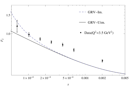
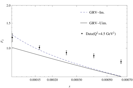
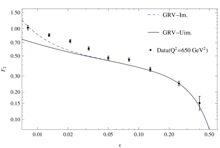
Figure 2: Our results for the modified nucleon structure function(NSF) , $F_{2}(x)$, at $Q^{2}=3.5\;GeV^{2}$, $4.5\;GeV^{2}$ and $650\;GeV^{2}$ which are compared with the available experimental data  [64] and the normal GRV parametrization model  [51]. Here the ”GRV-Im.” is indicating our results for the modified NSF, using GRV model. The ”GRV-Uim.” symbol is denoting the normal NSF in GRV model.

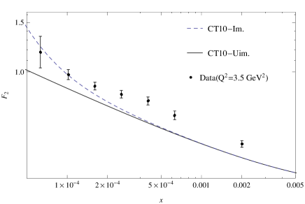
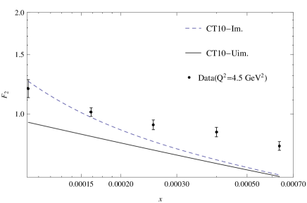
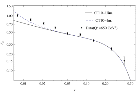
Figure 3: Our results for the modified nucleon structure function(NSF) , $F_{2}(x)$, at $Q^{2}=3.5\;GeV^{2}$, $4.5\;GeV^{2}$ and $650\;GeV^{2}$ which are compared with the available experimental data  [64] and the normal CT10 parametrization model  [53]. Here the ”CT10-Im.” is indicating our results for the modified NSF, using CT10 model. The ”CT10-Uim.” symbol is denoting the normal NSF in CT10 model.

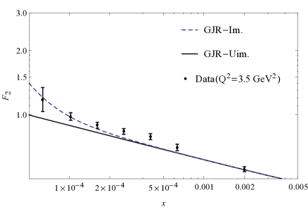
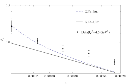
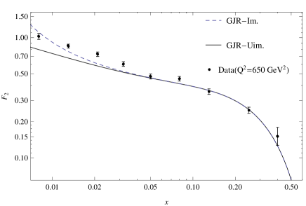
Figure 4: Our results for the modified nucleon structure function(NSF) , $F_{2}(x)$, at $Q^{2}=3.5\;GeV^{2}$, $4.5\;GeV^{2}$ and $650\;GeV^{2}$ which are compared with the available experimental data [64] and the normal GJR(JR09FFNNLO) parametrization model [52]. Here the ”GJR(JR09FFNNLO)-Im.” is indicating our results for the modified NSF, using GJR model. The ”GJR(JR09FFNNLO)-Uim.” symbol is denoting the normal NSF in CT10 model.

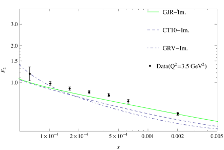
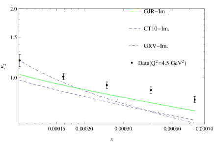
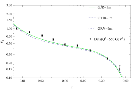
Figure 5: Our results for the modified nucleon structure function(NSF) , $F_{2}(x)$, at $Q^{2}=3.5\;GeV^{2}$, $4.5\;GeV^{2}$ and $650\;GeV^{2}$ which are compared with the available experimental data [64], using GRV, CT10 and GJR(JR09NNLO) models.

To plot the $F_{2}(x)$ we need two NC parameters, $\Lambda_{NC}$ and $K_{\gamma gg}$. good fits for $F_{2}$ with experimental date is obtained for approved amounts of energy scale $\Lambda_{NC}$. As it has been mentioned above, looking for the literature and concerned articles, there is not specific value for the NC scale. Collider scattering experiments could be a proper evident to search NCST effects because they are very sensitive to NC signals. Usual bound from these experiments is $\Lambda_{NC}\sim 1TeV$. Present work is also implemented for collider scattering experiment to find modified structure functions of nucleons in NCST. So we have also employed this range that is prevalent in such processes.

Following the procedure which was described in the expanded approach, one can find three numerical values for the $K_{\gamma gg}$ parameter which are -0.098, 0.197 and -0.396 respectively [60, 61]. $\Lambda_{NC}$. Therefore we investigate these effects. The results for all three values of $K_{\gamma gg}$ are similar to each other. Therefore we just present the results coming from the numerical values of parameters and scales which are tabulated in table 1. As can be seen from table 1, the numerical value for NC scale is growing by increasing the $Q^{2}$ as squared transfer momentum. For example for a fixed $K_{\gamma gg}$, the $\Lambda_{NC}=800\;GeV$ for $Q^{2}=3.5\;GeV^{2}$ while for $Q^{2}=650\;GeV^{2}$ the $\Lambda_{NC}$ scale is equal to $2200\;GeV$. It is in correspond to our expectation from the NC effect. The $\Lambda_{NC}$ also depends on the measure of $K_{\gamma gg}$ parameter. According to table 2 for a fixed $Q^{2}$, the value of $\Lambda_{NC}$ increases when the magnitude of $K_{\gamma gg}$ is coming up. For instance, at a fixed $Q^{2}$ for $K_{\gamma gg}=-0.098$ we will get $\Lambda_{NC}=2200\;GeV$ and it is $4400\;GeV$ for $K_{\gamma gg}=-0.396$. The numerical values for NC scale, using the GJR and CT10 parametrization models are at the same order of the ones in tables 1 and 2 with similar behaviour.when the squared transfer momentum is increasing.

$Q^{2}(GeV)^{2}$	$K_{\gamma gg}$	$\Lambda_{NC}(GeV)$
$3.5$	$-0.098$	$830$
$4.5$	$-0.098$	$750$
$650$	$-0.098$	$2200$

Table 1: $\Lambda_{NC}$ variations with squared transfer momentum for a fixed $K_{\gamma gg}=-0.098$

$Q^{2}$ $(GeV)^{2}$	$K_{\gamma gg}$	$\Lambda_{NC}(GeV)$
$650$	$-0.098$	$2200$
$650$	$+0.197$	$3200$
$650$	$-0.396$	$4400$

Table 2: $\Lambda_{NC}$ variations with parameter $K_{\gamma gg}$ for a fixed $Q^{2}=650(GeV)^{2}$

Figures 2, 3 and 4 indicate good compatibility with experimental data especially for small values of $x$-Bjorken variable where we are expecting the effect of new physics are more relevant. To confirm the validity of our obtained results we can act conversely and concentrate to extract the energy scale, $\Lambda_{NC}$. We then need to consider Eq.( 4.1) while the energy scale, $\Lambda_{NC}$ is unknown. If, at the fixed $K_{\gamma gg}$, we use experimental data at low $Q^{2}$, a small value for $\Lambda_{NC}$ is obtained and for data at the highest $Q^{2}$ value a large value for $\Lambda_{NC}$ would be appeared. What we get are as following:

• For $K_{\gamma gg}=-0.098$:  $\Lambda_{NC}\geq 430\;GeV$

• For $K_{\gamma gg}=0.197$:     $\Lambda_{NC}\geq 610\;GeV$

• For $K_{\gamma gg}=-0.396$:  $\Lambda_{NC}\geq 860\;GeV$

However in obtaining the above numerical values for $\Lambda_{NC}$ scale we use the GRV model but similar results will be appeared when we employ the GJR and CT10 models. To do a confirmation on the validity of our calculations, we once again back to the Drell-Yan process which is an important role for investigating the nucleon structure function and in testing the parton model. Analysing this processes at the NCST will yield us $\Lambda_{NC}\geq 0.4\;TeV$ [31] which is compatible with what we get in this paper.

5 Conclusion

We have considered the effect of NCST on proton structure functions. There are two approaches to construct the usable NC theory. In both approaches, all present vertices are modified by the NC parameter $\theta_{\mu\nu}$. In this case, in addition to the usual interactions, some new interactions would also be appeared. We have applied two new corrections and two new interactions, one for each approach, to calculate the structure functions of proton. Three of the four corrections do not have any effect, but new interaction from expanded approach contributes to the nucleon structure function. As can be seen, the obtained results for the improved proton structure function, $F_{2}(x)$ , are in better compatibility with available experimental data rather than the results coming from the normal GRV, CT10 and GJR parametrization models, specially at small values of $x$-Bjorken variable which is related to the high energy region. Also the magnitude order of NC energy scale that we got, using NCSM approach, is correspond to the expected range of the other predictions.

In this paper we considered a spacial case when $\theta_{\mu 0}=0$ but one can calculate the case for $\theta_{\mu 0}\neq 0$ which we hope to report about it in future. The current results can be extended to the higher order approximation which we hope to do it as our new research task. The NCSM which we used it here, contained the lorentz violation. Some similar calculations in which lorentz invariant is conserved can be done which we hope to report on this issue latter on.

Appendix A Appendix

Here, we perform the required calculations for electron-quark and electron-gluon scattering in the expanded NC in details. Similar calculations can be done for unexpanded NC.

Electron-quark scattering: Employing Feynman rule for figure 1 we will able to obtain the required results up to leading order, considering the NC parameter. Since propagators do not affected by NC corrections therefore just vertexes should be written in NC space-time. According to photon-fermion vertex in laboratory system (see Eq.( 3.2)), invariant amplitude read as it follow:

$$\begin{array}[]{l}{-i\cal{M}}=[\bar{u}(k^{\prime})(i{g_{e}}{\gamma^{\mu}})u(k)][\frac{{-i{g_{\mu\nu}}}}{{{q^{2}}}}][\bar{u}(p^{\prime})(i{e_{i}}{g_{e}}{\gamma^{\nu}})u(p)]\\ \quad\quad\;\;+[\bar{u}(k^{\prime})(i{g_{e}}{\gamma^{\mu}})u(k)][\frac{{-i{g_{\mu\nu}}}}{{{q^{2}}}}][\bar{u}(p^{\prime})(\frac{1}{2}{e_{i}}{g_{e}}{C^{\nu}})u(p)].\end{array}$$ (A.1)

Doing some simplification we will have:

$$\begin{array}[]{l}{-\cal{M}}=\frac{{{e_{i}}g_{e}^{2}}}{{{q^{2}}}}[\bar{u}(k^{\prime}){\gamma^{\mu}}u(k)][\bar{u}(p^{\prime}){\gamma_{\mu}}u(p)]\\ \quad\quad-i\frac{{{e_{i}}g_{e}^{2}}}{{2{q^{2}}}}[\bar{u}(k^{\prime}){\gamma^{\mu}}u(k)][\bar{u}(p^{\prime}){C_{\mu}}u(p)].\end{array}$$ (A.2)

Then for the squared invariant amplitude, we will get:

$$\begin{array}[]{l}{{\left|\cal{M}\right|^{2}}}={(\frac{{{e_{i}}g_{e}^{2}}}{{{q^{2}}}})^{2}}[\bar{u}(k^{\prime}){\gamma^{\mu}}u(k)][\bar{u}(p^{\prime}){\gamma_{\mu}}u(p)]{[\bar{u}(k^{\prime}){\gamma^{\nu}}u(k)]^{\dagger}}\\ {[\bar{u}(p^{\prime}){\gamma_{\nu}}u(p)]^{\dagger}}+\frac{i}{2}{(\frac{{{e_{i}}g_{e}^{2}}}{{{q^{2}}}})^{2}}[\bar{u}(k^{\prime}){\gamma^{\mu}}u(k)][\bar{u}(p^{\prime}){\gamma_{\mu}}u(p)]\\ {[\bar{u}(k^{\prime}){\gamma^{\nu}}u(k)]^{\dagger}}{[\bar{u}(p^{\prime}){C_{\nu}}u(p)]^{\dagger}}-\frac{i}{2}{(\frac{{{e_{i}}g_{e}^{2}}}{{{q^{2}}}})^{2}}{[\bar{u}(k^{\prime}){\gamma^{\mu}}u(k)]}\\ {[\bar{u}(p^{\prime}){C_{\mu}}u(p)]}{[\bar{u}(k^{\prime}){\gamma^{\nu}}u(k)]^{\dagger}}{[\bar{u}(p^{\prime}){\gamma_{\nu}}u(p)]^{\dagger}}.\end{array}$$ (A.3)

Here, we remember that for two $4\times 4$ ${\Gamma_{1}}$ and ${\Gamma_{2}}$ matrices, Casimir’s trick will lead us to:

$$\begin{array}[]{l}\sum\limits_{all\;spins}{[\bar{u}(a){\Gamma_{1}}u(b)]{{[\bar{u}(a){\Gamma_{2}}u(b)]}^{\dagger}}}=\\ \qquad\qquad\qquad Tr[\,{\Gamma_{1}}\,({\not p_{b}}+{m_{b}})\,{\bar{\Gamma}_{2}}({\not p_{a}}+{m_{a}})]\;.\end{array}$$ (A.4)

According to ${\bar{\Gamma}_{2}}={\gamma^{0}}\Gamma_{2}^{\dagger}\,{\gamma^{0}}$ definition, we have: ${\gamma^{0}}{C^{\nu{\dagger}}}\,{\gamma^{0}}=-{C^{\nu}}$, ${\gamma^{0}}{\gamma^{\nu{\dagger}}}\,{\gamma^{0}}={\gamma^{\nu}}$. Now by taking average over initial spin states and sum over final spin states and using the Casimir’s trick we arrive at Eq.( 3.3).

Electron-gluon scattering: To do the required calculations, we consider figure 1 and proceed to do the square of invariant amplitude in Eq.( 3.8). Then doing the average over initial spins states and sum over final spin states and then gluon polarization states so as:

$$\sum{{\varepsilon_{\mu}}\varepsilon_{\nu}^{*}}\to-{g_{\mu\nu}},$$ (A.5)

and color algebra

$$\sum\limits_{{c_{1}}{c_{2}}}{{\delta^{{c_{1}}{c_{2}}}}{\delta_{{c_{1}}{c_{2}}}}}=\sum\limits_{{c_{1}}=1}^{8}{{\delta^{{c_{1}}{c_{1}}}}}=8,$$ (A.6)

we will get the following result:

$$\begin{array}[]{l}\left\langle{{\left|\cal{M}\right|}^{2}}\right\rangle=\frac{16{N^{2}}g_{e}^{4}}{q^{4}}\left[\theta^{2}\left(k.k^{\prime}\,(p^{2}+q^{2})(-p^{2}q^{2}+(q.p)^{2})\right.\right.\\ \left.\left.-q^{2}q.p\,(k.pk^{\prime}.q+k.qk^{\prime}.p)+q^{4}k.p\,k^{\prime}.p+k.q\,k^{\prime}.q\,(q.p)^{2}\right.\right.\\ \left.\left.-k.k^{\prime}\,q.p\,(p^{2}q^{2}-(q.p)^{2})\right)-p^{4}k.\theta.q\,k^{\prime}.\theta.q+k.\theta.\theta.q\right.\\ \left.\times(q^{2}p^{2}\,k^{\prime}.(q+p))+k.\theta.\theta.k^{\prime}(p^{2}+(p+q)^{2})(p^{2}q^{2}\right.\\ \left.-(p.q)^{2})-q.\theta\theta.q\left(p^{2}\,k.k^{\prime}(\frac{p^{2}}{2}+2q^{2}+3q.p)+k.pk^{\prime}.p\right.\right.\\ \left.\left.(2p^{2}+q^{2}+2p.q)+(k.qk^{\prime}.p+k.p\,k^{\prime}.q)(p^{2}+2p.q)\right)\right.\\ \left.-p^{2}k.qk^{\prime}.q+k^{\prime}.\theta.\theta.q\left((q^{2}\,p^{2}-2(q.p)^{2})k.(p+q)\right)\right.\\ \left.\left.+(p^{2}\,k.q+q^{2}\,k.p)\,q.p\right)\right]\end{array}$$ (A.7)

In Eq.( A.7) we neglected from electron mass. We note that since there is not more than two gluon legs, thus incident gluon is like the outgoing gluon. Mathematically, the delta Kronecker function confirms this reality. On the other hand since gluons are appearing in eight color states, we should consider the color factor in our calulation which can be done, using Eq.( A.6). Now to simplify the above equation, by takeing $\alpha$, $\beta$, $\gamma$ as angles between $\vec{k}$, $\vec{k}^{\prime}$, $\vec{k}\times\vec{k}^{\prime}$ and $\vec{\theta}$ direction, respectively, in the laboratory system and using Eqs.( 2.7) and ( 2.8) we will get:

$$k.\,\theta.\,\theta.\,k={E^{2}}|\vec{\theta}{|^{2}}{\sin^{2}}\alpha,$$ (A.8)

$$k^{\prime}.\,\theta.\,\theta.\,k^{\prime}={E^{\prime 2}}|\vec{\theta}{|^{2}}{\sin^{2}}\beta,$$ (A.9)

$$k.\,\theta.\,\theta.\,k^{\prime}=E\,E^{\prime}|\vec{\theta}{|^{2}}(\cos\varphi-\cos\beta\cos\alpha),$$ (A.10)

$$k.\,\theta.\,k^{\prime}=E\,E^{\prime}|\vec{\theta}|\sin\varphi\cos\gamma\;.$$ (A.11)

Then by taking the average over $\alpha$, $\beta$ and $\gamma$, Eq.( A.7) will lead us to:

$$\left\langle{{{\left|\cal{M}\right|}^{2}}}\right\rangle=\frac{{8{N^{2}}g_{e}^{4}}}{{{q^{4}}}}{\theta^{2}}EE^{\prime}m_{eff}^{2}\left[{a^{\prime}{{\cos}^{2}}(\frac{\varphi}{2})+b^{\prime}{{\sin}^{2}}(\frac{\varphi}{2})}\right],$$ (A.12)

where

$$\begin{array}[]{l}a^{\prime}=-12{m_{eff}}{E^{3}}-6m_{eff}^{2}{E^{2}}+12{E^{2}}{Q^{2}}-5m_{eff}^{2}{Q^{2}}\\ \quad+6{Q^{4}}+40{m_{eff}}{E^{2}}E^{\prime}+16m_{eff}^{2}EE^{\prime}-40{m_{eff}}E{{E^{\prime}}^{2}}\\ \quad-22EE^{\prime}{Q^{2}}-6m_{eff}^{2}{{E^{\prime}}^{2}}+12{{E^{\prime}}^{2}}{Q^{2}}+12{m_{eff}}{{E^{\prime}}^{3}},\end{array}$$ (A.13)

$$\begin{array}[]{l}b^{\prime}=-8{E^{4}}-8{{E^{\prime}}^{4}}+4{m_{eff}}{E^{3}}+2m_{eff}^{2}{E^{2}}\\ \quad+4m_{eff}^{2}{Q^{2}}-24{m_{eff}}{E^{2}}E^{\prime}-6m_{eff}^{2}EE^{\prime}\\ \quad-4EE^{\prime}{Q^{2}}+24{m_{eff}}E{{E^{\prime}}^{2}}+2m_{eff}^{2}{{E^{\prime}}^{2}}\\ \quad+\frac{{11{Q^{4}}}}{4}-4{m_{eff}}{{E^{\prime}}^{3}}.\end{array}$$ (A.14)

Here ${m_{eff}}$ is zeroth component of four-momentum for gluon. By substitute Eq.( A.12) into below equation

$$\begin{array}[]{l}d\sigma=\frac{1}{{(2E)(2m)}}\frac{{\left\langle{{{\left|\cal{M}\right|}^{2}}}\right\rangle}}{{4{\pi^{2}}}}\frac{{{d^{3}}k^{\prime}}}{{2E^{\prime}}}\frac{{{d^{3}}p^{\prime}}}{{2{{p^{\prime}}_{0}}}}{\delta^{(4)}}(p+k-p^{\prime}-k^{\prime})\\ \quad\;\;=\frac{1}{{4mE}}\frac{{\left\langle{{{\left|\cal{M}\right|}^{2}}}\right\rangle}}{{4{\pi^{2}}}}\frac{1}{2}E^{\prime}dE^{\prime}d\Omega\frac{{{d^{3}}p^{\prime}}}{{2{{p^{\prime}}_{0}}}}{\delta^{(4)}}(p+k-p^{\prime}-k^{\prime}),\end{array}$$ (A.15)

and using

$$\int{\frac{{{d^{3}}p^{\prime}}}{{2{{p^{\prime}}_{0}}}}{\delta^{(4)}}(p+q-p^{\prime})}=\frac{1}{{2m}}\delta(\nu+\frac{{{q^{2}}}}{{2m}}),$$ (A.16)

where in laboratory system we have

$$d(\cos\varphi)dE^{\prime}=\frac{1}{{2EE^{\prime}}}d{Q^{2}}d\nu,$$ (A.17)

we obtain

$$\begin{array}[]{l}\frac{{d\sigma}}{{d{Q^{2}}d\nu}}=\frac{{\pi{\alpha^{2}}}}{{4{E^{2}}{{\sin}^{4}}(\frac{\varphi}{2})}}\frac{1}{{EE^{\prime}}}\\ \qquad\qquad\left[{a\,{{\cos}^{2}}(\frac{\varphi}{2})+b{{\sin}^{2}}(\frac{\varphi}{2})}\right]\delta(\nu-\frac{{{Q^{2}}}}{{2{m_{eff}}}}).\end{array}$$ (A.18)

Here $a=\frac{{{N^{2}}{\theta^{2}}}}{{2}}a^{\prime}$ and $b=\frac{{{N^{2}}{\theta^{2}}}}{{2}}b^{\prime}$. Now, by comparing Eqs.( A.18) and ( 3.1), we can determine gluon contributions to the nucleon structure function which are denoted by $w_{1}^{gluon}$ and $w_{2}^{gluon}$ respectively:

$$w_{1}^{gluon}=\frac{b}{2}\delta(\nu-\frac{{{Q^{2}}}}{{2M\,{x_{g}}}}),$$ (A.19)

$$w_{2}^{gluon}=a\,\delta(\nu-\frac{{{Q^{2}}}}{{2M\,{x_{g}}}}),$$ (A.20)

in which we use ${m_{eff}}={x_{g}}M$. Here ${x_{g}}$ is fraction of nucleon momentum which is carried by gluon. To obtain nucleon structure function which is resulted from electron-gluon scattering, it is needed to multiply $w_{1}^{gluon}$ and $w_{2}^{gluon}$ by $g({x_{g}})$, as probability function to find gluon with fraction of nucleon’s momentum. Then taking integrate with respect to ${x_{g}}$ would be resulted to:

$$\begin{array}[]{l}{W_{1}}({Q^{2}},\nu)=\int\limits_{0}^{1}{d{x_{g}}g({x_{g}})w_{1}^{gluon}}\\ \qquad\qquad\;\;=\int\limits_{0}^{1}{d{x_{g}}g({x_{g}})\frac{{b({x_{g}})}}{2}\delta(\nu-\frac{{{Q^{2}}}}{{2M{x_{g}}}})}\\ \qquad\qquad{\kern 1.0pt}=\int\limits_{0}^{1}{d{x_{g}}g({x_{g}})\frac{{b({x_{g}})}}{2}\frac{{{x_{g}}}}{\nu}\delta({x_{g}}-x)}\\ \qquad\qquad{\kern 1.0pt}=\frac{{b(x)}}{2}\frac{x}{\nu}g(x)=\frac{{b(x)}}{M}\frac{{{M^{2}}x}}{{{Q^{2}}}}g(x),\end{array}$$ (A.21)

$$\begin{array}[]{l}{W_{2}}({Q^{2}},\nu)=\int\limits_{0}^{1}{d{x_{g}}g({x_{g}})w_{2}^{gluon}}\\ \qquad\qquad\;\;=\int\limits_{0}^{1}{d{x_{g}}g({x_{g}})\,a({x_{g}})\,\delta(\nu-\frac{{{Q^{2}}}}{{2M{x_{g}}}})}\\ \qquad\qquad{\kern 1.0pt}=\int\limits_{0}^{1}{d{x_{g}}g({x_{g}})\,a({x_{g}})\frac{{{x_{g}}}}{\nu}\delta({x_{g}}-x)}\\ \qquad\qquad{\kern 1.0pt}=\frac{1}{\nu}a(x)\,x\,g(x),\end{array}$$ (A.22)

where Eqs.( 3.9, 3.10) as the corrected portion of structure function are coming from gluon-photon interaction.

References

• [1] A. Ghasempour Nesheli, A. Mirjalili, M. M. Yazdanpanah, Analyzing the parton densities and constructing the $xF_{3}$ structure function, using the Laguerre polynomials expansion and Monte Carlo calculations, Eur. Phys. J. Plus 130 (2015) 82.
• [2] A. Mirjalili, M. Dehghani , M.M. Yazdanpanah, Parton densities with the quark linear potential in the statistical approach, Int. J. Mod. Phys. A 28 (2013) 1350089.
• [3] M. Gluck, E. Reya, A. Vogt, Parton structure of the photon beyond the leading order, Phys. Rev. D 45 (1992) 3986.
• [4] V Vikhrov et al., Flavor decomposition of the sea quark helicity distributions in the nucleon from semiinclusive deep inelastic scattering, Phys. Rev. Lett. 92 (2004) 012005.
• [5] A.D. Martin, W.J. Stirling, R.S. Thorne and G. Watt, Parton distributions for the LHC, Eur. Phys. J. C 63 (2009) 189.
• [6] F.D. Aaron et al., The H1 and ZEUS collaborations, Combined measurement and QCD analysis of the inclusive $e^{\pm}p$ scattering cross sections at HERA, JHEP 01 (2010) 109.
• [7] J. Gao et al., CT10 next-to-next-to-leading order global analysis of QCD, Phys. Rev. D 89 (2014) 033009.
• [8] J. Peng, J.W. Qiu, Novel phenomenology of parton distributions from the Drell-Yan process, Prog. Part. Nucl. Phys 76 (2014) 43.
• [9] E. Witten, Non-commutative geometry and string field theory, Nucl. Phys. B 268 (1986) 253.
• [10] N. Seiberg, E. Witten, String theory and noncommutative geometry, JHEP 09 (1999) 032.
• [11] S. Bilmis et al., Constraints on a noncommutative physics scale with neutrino-electron scattering, Phys. Rev. D 85 (2012) 073011.
• [12] M. Chaichian, M. M. Sheikh-Jabbari, A. Tureanu, Hydrogen atom spectrum and the lamb shift in noncommutative QED, Phys. Rev. Lett. 86 (2001) 2716.
• [13] H.N. Brown et al., Precise measurement of the positive muon anomalous magnetic moment, Phys. Rev. Lett. 86 (2001) 2227.
• [14] X.J. Wang, M.L. Yan, Noncommutative QED and muon anomalous magnetic moment, JHEP 0203 (2002) 047.
• [15] N. Kersting, Muon g-2 from noncommutative geometry, Phys.Lett. B 527 (2002) 115.
• [16] I. Mocioiu, M. Pospelov and R. Roiban, Limits on the non-commutativity scale, arXiv:hep-ph/0110011.
• [17] S.M.Carroll et al., Noncommutative field theory and Lorentz violation, Phys. Rev. Lett. 87 (2001) 141601.
• [18] M. Haghighat, F. Loran, Three body bound state in non-commutative space, Phys. Rev. D 67 (2003) 096003.
• [19] M. Buric et al., Nonzero $Z\rightarrow\gamma\gamma$ decays in the renormalizable gauge sector of the noncommutative standard model, Phys. Rev. D 75 (2007)097701.
• [20] M.M. Najafabadi, Noncommutative standard model in top quark sector, Phys. Rev. D 77 (2008) 116011.
• [21] M. Mohammadi Najafabadi, Semileptonic decay of a polarized top quark in the noncommutative standard model, Phys. Rev. D 74 (2006) 025021.
• [22] N. Mahajan, $t\rightarrow bW$ in noncommutative standard model, Phys. Rev. D 68 (2003) 095001.
• [23] P. Mathews, Compton scattering in noncommutative space-time at the NLC, Phys. Rev. D 63 (2001) 075007.
• [24] G. Abbiendi et al., Test of non-commutative QED in the process $e^{+}e^{-}\rightarrow\gamma\gamma$ at LEP, Phys. Lett. B 568 (2003) 181.
• [25] P. Schupp et al., The Photon neutrino interaction in noncommutative gauge field theory and astrophysical bounds, Eur. Phys. J. C 36 (2004) 405.
• [26] R. Horvat, J. Trampetic, Constraining spacetime noncommutativity with primordial nucleosynthesis, Phys. Rev. D 79 (2009) 087701.
• [27] R. Horvat, D. Kekez, J. Trampetic, Spacetime noncommutativity and ultra-high energy cosmic ray experiments, Phys. Rev. D 83 (2011) 065013.
• [28] J. L. Hewett, F. J. Petriello, T. G. Rizzo, Signals for noncommutative interactions at linear colliders, Phys. Rev. D 64 (2001) 075012.
• [29] A. Alboteanu, T. Ohl, R. Ruckl, Probing the noncommutative standard model at hadron colliders, Phys. Rev. D 74 (2006) 096004.
• [30] T. Ohl, C. Speckner, The Noncommutative standard model and polarization in charged gauge boson production at the LHC, Phys. Rev. D 82 (2010) 116011.
• [31] J. Selvaganapathy, P. K. Das, P. Konar, Drell-Yan process as an avenue to test a noncommutative standard model at the Large Hadron Collider, Phys. Rev. D 93 (2016) 116003.
• [32] M. Chaichian et al., Noncommutative standard model: Model building, Eur. Phys. J. C 29 (2003) 413.
• [33] X. Calmet et al., The Standard model on noncommutative space-time, Eur. Phys. J. C 23 (2002) 363.
• [34] B. Melic et al., The Standard model on non-commutative space-time: Electroweak currents and the Higgs sector, Eur. Phys. J. C 42 (2005) 483.
• [35] B. Melic et al., The Standard model on non-commutative space-time: Strong interactions included, Eur. Phys. J. C 42 (2005) 499.
• [36] M. M. Ettefaghi, M. Haghighat, R. Mohammadi, Noncommutative QED+QCD and the $\beta$ function for QED, Phys. Rev. D 82 (2010) 105017.
• [37] S. Batebi et al., Higgs couplings in noncommutative standard model, Int. J. Mod. Phys. A 30 (2015) 1550108.
• [38] E. Bavarsad et al., Generation of circular polarization of the CMB, Phys. Rev. D 81 (2010) 084035.
• [39] J. Selvaganapathy, P. K. Das, P. Konar, Search for associated production of Higgs with Z boson in the noncommutative standard model at linear colliders, Int. J. Mod. Phys. A 30 (2015) 1550159.
• [40] J. Trampetic, High energy cosmic rays experiments inspired by noncommutative quantum field theory, arXiv:1210.5427.
• [41] J. Trampetic, Photon-neutrino interaction in theta-exact covariant noncommutative model: Phenomenology and Quantum properties, Int. J. Geom. Meth. Mod. Phys. 09 (2012) 1261016.
• [42] M. Haghighat, M.Khorsandi, Hydrogen and muonic hydrogen atomic spectra in non-commutative space-time, Eur. Phys. J. C 75 (2015) 4.
• [43] A. Joseph, Particle phenomenology on noncommutative spacetime, Phys. Rev. D 79 (2009) 096004.
• [44] P.K. Das, N.G. Deshpande, G. Rajasekaran, M ller and Bhabha scattering in the noncommutative standard model, Phys. Rev. D 77 (2008) 035010.
• [45] M. M. Ettefaghi, Two-photon annihilation of singlet cold dark matter due to noncommutative space-time, Phys. Rev. D 86 (2012) 085038.
• [46] M. M. Ettefaghi, Singlet particles as cold dark matter in a noncommutative space-time, Phys. Rev. D 79 (2009) 065022.
• [47] M. Ghasemkhani et al., Higgs production in $e^{-}e^{+}$ collisions as a probe of noncommutativity, Prog. Theo. Exp. Phys (2014) 081B01.
• [48] B. Melic, K. Passek-Kumericki, J. Trampetic, $K\rightarrow\pi\gamma$ decays and space-time noncommutativity, Phys. Rev. D 72 (2005) 057502.
• [49] J. A. Conley, J. L. Hewett, Effects of the noncommutative standard model in $WW$ scattering, arXiv:0811.4218.
• [50] A. Anisimov et al., Remarks on noncommutative phenomenology, Phys.Rev. D 65, 085032 (2002).
• [51] M. Gluck, E. Reya, A. Vogt, Dynamical parton distributions of the proton and small-x physics, Z. Physik C 67 (1995) 433.
• [52] P. Jimenez-Delgado, E. Reya, Dynamical next-to-next-to-leading order parton distributions, Phys. Rev. D 79 (2009) 074023.
• [53] Hung-Liang Lai et al., New parton distributions for collider physics, Phys. Rev. D 82 (2010) 074024.
• [54] J. Madore et al., Gauge theory on noncommutative spaces, Eur. Phys. J. C 16 (2000) 161.
• [55] I.F. Riad, M.M. Sheikh-Jabbari, Noncommutative QED and anomalous dipole moments, JHEP 0008 (2000) 045.
• [56] M. Hayakawa, Perturbative analysis on infrared aspects of noncommutative QED on R**$4$, Phys. Lett. B 478 (2000) 394.
• [57] M. Hayakawa, Perturbative analysis on infrared and ultraviolet aspects of noncommutative QED on R**$4$, arXiv:hep-th/9912167
• [58] M. Chaichian et al., Noncommutative gauge field theories: A no go theorem, Phys. Lett. B 526 (2002) 132 .
• [59] J. Gomis, T. Mehen, Space time noncommutative field theories and unitarity, Nucl. Phys. B 591 (2000) 265.
• [60] W. Behr et al., The $Z\rightarrow\gamma\gamma$, gg decays in the noncommutative standard model, Eur. Phys. J. C 29 (2003) 441.
• [61] N. G. Duplancic, P. Schupp, J. Trampetic, Comment on triple gauge boson interactions in the non-commutative electroweak sector, Eur. Phys. J. C 32 (2003) 141.
• [62] W. Greiner, S.Schramm and E.Stein, Quntum chromo dynamic, Third Ed., Speringer (2007).
• [63] F. Halzen and A.D.Martin, Quarks and Leptons: An introductory course in modern particle physics, Jhon Wiley and Sons (1987).
• [64] ZEUS Collaboration, S. Chekanov et al., Measurement of the neutral current cross section and ${F_{2}}$ structure function for deep inelastic scattering at HERA, Eur. Phys. J. C 21 (2001) 443.