Assignment of fields from particles to mesh

Abstract

In Computational Fluid Dynamics there have been many attempts to combine the power of a fixed mesh on which to carry out spatial calculations with that of a set of particles that moves following the velocity field. These ideas indeed go back to Particle-in-Cell methods, proposed about 60 years ago. Of course, some procedure is needed to transfer field information between particles and mesh. There are many possible choices for this “assignment”, or “projection”. Several requirements may guide this choice. Two well-known ones are conservativity and stability, which apply to volume integrals of the fields. An additional one is here considered: preservation of information. This means that mesh interpolation, followed by mesh assignment, should leave the field values invariant. The resulting methods are termed “mass” assignments due to their strong similarities with the Finite Element Method. We test several procedures, including the well-known FLIP, on three scenarios: simple 1D convection, 2D convection of Zalesak’s disk, and a CFD simulation of the Taylor-Green periodic vortex sheet. The most symmetric mass assignment is seen to be clearly superior to other methods.

1 Introduction

Historically, there have been two points of view to consider the dynamics of fluids: Eulerian, describing the dynamics of fluid with respect to an external frame, and Lagrangian, describing its dynamics within the flow. These approached would be reflected in computational fluid dynamics (CFD), in which the discretization may be carried out on a fixed, Eulerian, mesh, or on a Lagrangian moving set of computational particles. Each approach has its advantages and drawbacks.

The idea of combining both approaches goes back to Particle-in-Cell (PIC) methods, introduced in the 1950s [11, 10, 1]. The hope was to carry out the numerically expensive calculations related to spatial derivatives on a fixed mesh. The velocity field would then be transferred to particles, which would move according to it, advecting other fields. These would be transferred back to the mesh to begin the next iteration.

This very appealing idea also has its drawbacks. The obvious one is that a new procedure is needed to transfer the field information between particles and mesh. This procedure has been termed “assignment”. We will here use “projection” as a synonym. Our main task is to study the performance of different projection techniques, under the guidance of several requirements. One of them is conservativity: the total volume integral of a field must not vary upon projection. Another is stability: the integral of the square of any field should decrease upon projection. These two are well known, while here we consider an additional one: preservation of information. This means that the field values at discrete points do not vary under projection interpolation followed by projection.

The article is organized as follows. In Section 2 assignment procedures are discussed. First, conservativity and stability are defined in Section 2.1. Then, the simplest assignment is seen introduced in 2.2. The FLIP procedure, which is currently very popular in the computer graphics community [2] is considered in 2.3. In Section 2.4 we provide a discussion of the mass assignment idea, and its possible variants. These procedures are then tested in three scenarios in Section 3. The first one, in Section 3.1, is a very simple 1D convection of a top-hat function. This is actually a 1D version of the well known Zalesak’s disk 2D test, which is considered in 3.2. Finally, a CFD simulation of the Taylor-Green periodic vortex sheet, a solution of the Navier-Stokes equations, is given in Section 3.3. Some finishing remarks are given in Section 4.

2 Assignment procedures

The set of functions $\{\psi_{\mu}\}$ is used to interpolate, or reconstruct, a field $A(\mathbf{r})$ from its values at particles $A_{\mu}$:

$$A(\mathbf{r})\doteq\sum_{\mu}A_{\mu}\psi_{\mu}(\mathbf{r}).$$ (1)

The functions are supposed to comply with partition of unity, in order a particle distribution with constant values yields a constant field:

$$\sum_{\mu}\psi_{\mu}(\mathbf{r})=1.$$ (2)

In this work, we will only consider the simple linear Finite Element basis functions (FEs), even though other choices are of course possible.

For the mesh we will keep the same symbols, but the subindices will be Latin letters. A field is reconstructed from the values at mesh nodes $\overline{A}_{i}$ by mesh functions $\{\psi_{i}\}$:

$$\overline{A}(\mathbf{r})\doteq\sum_{i}\overline{A}_{i}\psi_{i}(\mathbf{r}).$$ (3)

The particle-to-mesh assignment procedure consists of finding nodal values for $\overline{A}_{i}$ given particle values $A_{\mu}$. The inverse mesh-to-particle yields particle $\overline{\overline{A}}_{\mu}$ given mesh $\overline{A}_{i}$.

2.1 Conservativity and stability

An property that may lead us on our research of possible assignment methods is conservativity. This expresses that the integral of a field will not change upon projection. Integrating field $A$ of Eq. (1),

$$\int A(\mathbf{r})d\mathbf{r}=\sum_{\mu}A_{\mu}v_{\mu},$$

where particle volumes are given by

$$v_{\mu}:=\int\psi_{\mu}(\mathbf{r})d\mathbf{r}.$$ (4)

Equivalently, mesh volumes may be defined from Eq. (3),

$$v_{i}:=\int\psi_{i}(\mathbf{r})d\mathbf{r}.$$ (5)

However, the FLIP method below does not use this mesh volume.

Whichever the particular definition of the volumes, conservativity is expressed as:

$$\sum_{i}\overline{A}_{i}v_{i}=\sum_{\mu}A_{\mu}v_{\mu}.$$ (6)

In the case of linear momentum components, this would guarantee the conservation of linear momentum. For a density field, this would guarantee conservation of mass. It therefore would seem as a vital requirement. However, we will see that methods that do not comply with this condition still may deviate little from it.

Of course, the same requirement could be asked when projecting from the mesh onto the particles:

$$\sum_{\mu}\overline{\overline{A}}_{\mu}v_{\mu}=\sum_{i}\overline{A}_{i}v_{i}.$$ (7)

Another requirement is stability: for any energy-like expression defined on the particles and on the mesh:

$$E_{\mathrm{p}}:=\sum_{\mu}v_{\mu}A_{\mu}^{2}\qquad E_{\mathrm{m}}:=\sum_{i}v_{i}\overline{A}_{i}^{2},$$

we require

$$E_{\mathrm{m}}\leq E_{\mathrm{p}}.$$ (8)

This guarantees that there is no overshoot in e.g. the kinetic energy upon assignment. Also, for a general field this forces a diminishing second momentum, which prevents overshooting in a global sense. Of course, the same could be required when going from the mesh to the particles.

2.2 $\delta$ assignment

The simplest assignment would be to define mesh values as the local values reconstructed from the particles:

$$\overline{A}_{i}=\overline{A}(\mathbf{r}_{i})=\sum_{\mu}A_{\mu}\psi_{\mu}(\mathbf{r}_{i}).$$ (9)

Also,

$$\overline{\overline{A}}_{\mu}=\overline{\overline{A}}(\mathbf{r}_{i})=\sum_{i}\overline{A}_{i}\psi_{i}(\mathbf{r}_{\mu}).$$ (10)

Particle volume may simply be defined as in (4) and (5). It is easy to check that this procedure does not satisfy either conservativity or stability. In Table 1 we will collect the relevant expressions for the methods considered.

method	part $\rightarrow$ mesh	mesh $\rightarrow$ part
$\delta$	$\displaystyle\overline{A}_{i}=\sum_{\mu}A_{\mu}\psi_{\mu}(\mathbf{r}_{i})$ (9 )
FLIP	$\displaystyle\overline{A}_{i}:=\sum_{\mu}A_{\mu}v_{\mu}\psi_{i}(\mathbf{r}_{\mu})/\sum_{\mu}v_{\mu}\psi_{i}(\mathbf{r}_{\mu})$ (11,12)	$\displaystyle\overline{\overline{A}}_{\mu}=\overline{\overline{A}}(\mathbf{r}_{i})=\sum_{i}\overline{A}_{i}\psi_{i}(\mathbf{r}_{\mu})$ (10)
mass-$\delta$	$\displaystyle\overline{A}_{i}:=\sum_{j}m_{ij}^{-1}\int d\mathbf{r}A(\mathbf{r})\phi_{j}(\mathbf{r})$ (13, 19)
full mass	$\displaystyle\overline{A}_{i}:=\sum_{j}m_{ij}^{-1}\int d\mathbf{r}A(\mathbf{r})\psi_{j}(\mathbf{r})$ (13, 19)	$\displaystyle\overline{\overline{A}}_{\mu}:=\sum_{\nu}m_{\mu\nu}^{-1}\int d\mathbf{r}\overline{A}(\mathbf{r})\psi_{\nu}(\mathbf{r})$ (20)
mass - lumped	$\displaystyle\overline{A}_{i}:=\sum_{j}m_{ij}^{-1}\int d\mathbf{r}A(\mathbf{r})\psi_{j}(\mathbf{r})$ (13, 19)	$\displaystyle\overline{\overline{A}}_{\mu}:=\frac{1}{v_{\mu}}\int d\mathbf{r}\overline{A}(\mathbf{r})\psi_{\mu}(\mathbf{r})$ (17)
lumped	$\displaystyle\overline{A}_{i}:=\frac{1}{v_{i}}\int d\mathbf{r}A(\mathbf{r})\psi_{i}(\mathbf{r})$ (13, 17)

Table 1: Features of the methods considered (left column), the procedure by which fields are projected from particles to mesh (middle column), and the reverse procedure (right column). References are given to relevant equations in the text. The last two methods have been considered but results are not given.

2.3 FLIP assignment

This procedure starts from the expression

$$\overline{A}_{i}:=\frac{1}{v_{i}}\sum_{\mu}A_{\mu}v_{\mu}\psi_{i}(\mathbf{r}_{\mu}).$$ (11)

The particle volumes may be defined as in (4). If (5) is used for the mesh volumes one, recovers the PIC expression [11, 10, 1].

The FLIP procedure proposes the alternative mesh volume:

$$v_{i}:=\sum_{\mu}v_{\mu}\psi_{i}(\mathbf{r}_{\mu}).$$ (12)

This procedure can be shown to satisfy both conservativity and stability.

A later projection onto the particles is exactly as in the $\delta$-assignment, Eq. (10), and this can be seen to again satisfy conservativity and stability.

This procedure may seem to be a great improvement since a simple change in the mesh volume restores conservativity and stability. It is also convenient to code, since the mesh functional set, $\{\psi_{i}\}$, is used for both particle to mesh assignment and its reverse. However, the volume of a nodal mesh (12) does not depend on the mesh itself, but on the particles around it. A node may even have a vanishing volume if no particles are close and the $\{\psi_{\mu}\}$ have compact support. Also, the two assignments, (10) and (11) are clearly unsymmetrical. A summary of the method is given in Table 1.

2.4 Mass assignment

Let us consider the assignment procedure

$$\overline{A}_{i}:=\int d\mathbf{r}A(\mathbf{r})\phi_{i}(\mathbf{r}).$$ (13)

Here, the assignment functional set $\{\phi_{i}(\mathbf{r})\}$ consists of normalized functions:

$$\int d\mathbf{r}\phi_{i}(\mathbf{r})=1,$$ (14)

so that a constant field yields constant mesh values. Notice the $\{\psi_{\mu}\}$ functions carry no physical units, but the $\{\phi_{\mu}\}$ have units of length^-d, where $d$ is the spatial dimension. The $\delta$ method is recovered as a special case if Dirac $\delta$ functions are used, $\phi_{i}(\mathbf{r})=\delta(\mathbf{r}-\mathbf{r}_{i})$, which in retrospect explains its name.

For conservativity, let us evaluate

$$\sum_{i}\overline{A}_{i}v_{i}=\sum_{i}\left(\int d\mathbf{r}A(\mathbf{r})\right)\phi_{i}(\mathbf{r})v_{i}=\int d\mathbf{r}A(\mathbf{r})\left(\sum_{i}\phi_{i}(\mathbf{r})v_{i}\right).$$ (15)

If the last parenthesis was equal to $1$, conservativity would apply (with particle volumes as in (4). Therefore, these functions must satisfy

$$\sum_{i}v_{i}\phi_{i}(\mathbf{r})=1.$$ (16)

If this condition holds, it is straightforward to proof that stability is also satisfied.

The simplest way to define these functions would be as normalized versions of the $\{\psi_{i}\}$ :

$$\phi_{i}(\mathbf{r})=\frac{1}{v_{i}}\psi_{i}(\mathbf{r})$$ (17)

This would correspond to a “lumped mass” method, a term that will become clear very soon.

Let us however consider $\{\phi_{i}\}$ that “preserves nodal information”. By this, we mean that a reconstruction procedure, followed by projection, should leave the nodal values invariant:

$$\overline{A}_{i}:=\int d\mathbf{r}\phi_{i}(\mathbf{r})\left(\sum_{j}\overline{A}_{j}\psi_{j}(\mathbf{r})\right).$$

(See also Ref. [7] , p. 243 for an application of this idea to an iterative method.) Notice these two operations are carried out on the mesh only (or, on particles only). This means

$$\int d\mathbf{r}\phi_{i}(\mathbf{r})\psi_{j}(\mathbf{r})=\delta_{ij},$$ (18)

where the latter $\delta$ is Kronecker’s. We will call this the “preservation property”. If the $\{\phi_{i}\}$ are linear combinations of the $\{\psi_{i}\}$ set, it is simple to show that

$$\phi_{i}(\mathbf{r})=\sum_{j}m_{ij}^{-1}\psi_{j}(\mathbf{r}),$$ (19)

where the inverse of the mass matrix appears, the latter defined as having elements

$$m_{ij}=:\int d\mathbf{r}\psi_{i}(\mathbf{r})\psi_{j}(\mathbf{r}).$$

It can be shown that the functions defined by (19) do comply with requirements (14) and (16). As a consequence, the resulting procedure will be conservative and stable.

For the sake of symmetry, a similar procedure is employed for projection onto the particles:

$$\overline{\overline{A}}_{\mu}:=\int d\mathbf{r}\overline{\overline{A}}(\mathbf{r})\phi_{\mu}(\mathbf{r}).$$ (20)

The resulting procedure can also be shown to satisfy both conservativity and stability.

Some remarks are in order.

First, the integration needed in (13) may be cumbersome to carry out. We therefore employ a simplified quadrature rule that involves a quadratic interpolation for function $\overline{A}(\mathbf{r})$, as explained below in Appendix B.

Second, this procedure requires matrix inversion. This is not such a problem for the mesh, since in a typical CFD computation these matrices must be assembled and inverted on the mesh anyway. On the particles however, such a calculation is often not needed, whereas it certainly is within the present procedure.

Third, the simple (17) would correspond to a lumped mass approximation in the language of the Finite Element Method (FEM). Indeed, $\sum_{j}m_{ij}=v_{i}$.

Fourth and last, there is an appealing correspondence with the usual FEM. Indeed, beginning with a Poisson equation:

$$g-\nabla^{2}A=0,$$

we may project onto a nodal functional space (it is immaterial for this discussion whether the following occurs on the particles, or on the mesh):

$$\sum_{i}g_{i}\psi_{i}(\mathbf{r})-\sum_{i}A_{i}\nabla^{2}\psi_{i}(\mathbf{r})\approx 0.$$

The equality is no longer satisfied in general, but we may ask the residual to be orthogonal to all the shape functions (as in the method of weighted residuals [14]):

$$\int d\mathbf{r}\left(\sum_{i}g_{i}\psi_{i}(\mathbf{r})-\sum_{i}A_{i}\nabla^{2}\psi_{i}(\mathbf{r})\right)\psi_{j}(\mathbf{r})=0\qquad\forall j.$$

This results in the expression

$$\sum_{i}m_{ij}g_{i}=\int d\mathbf{r}\psi_{j}(\mathbf{r})\nabla^{2}\left(\sum_{i}A_{i}\psi_{i}(\mathbf{r})\right).$$

Now, we may invert the mass matrix, and recalling our definition (19),

$$g_{j}=\int d\mathbf{r}\phi_{j}(\mathbf{r})\nabla^{2}\left(\sum_{i}A_{i}\psi_{i}(\mathbf{r})\right)=\int d\mathbf{r}\phi_{j}(\mathbf{r})\nabla^{2}\overline{A}(\mathbf{r})$$

This is an expression for the second derivative that entails: the reconstruction from the nodal values $A_{i}$ to a function $\overline{A}(\mathbf{r})$, deriving this function twice, then projecting back onto the nodes. We therefore see that a classical FEM approach yields an expression that is consistent with our mass assignment. Indeed, if the method to solve the equations of motion is of the FEM type, the calculations are already likely implemented in the code (at least, for the mesh).

We will consider two instances of mass projection. In the first one, mass projection will be used from the particles to the mesh, but simple $\delta$ projection will be used when projecting back. This is because in a typical pFEM-like simulation the matrices necessary for the former projection will be likely already computed, at the start of the simulation (they will not change since the mesh is fixed). If its performance was good, its numerical implementation would not imply a large increase in computational resources. We will call this method “mass-$\delta$”, for obvious reasons. The $\delta$ projection is not conservative nor stable, but we will see below that departs little from these requirements.

Our second choice will be “full mass” projection. This is the most symmetric mass assignment method, which will comply with conservativity and stability. It clearly requires the particle mass matrix must be calculated, and inverted, at each time step. We will see that this additional computational burden may be compensated by its superior performance.

Another possible candidate would be a “mass-lumped” method, where only the particle volumes are needed. Of course, a purely “lumped” method, both-ways, can be considered. These two lumped procedures are listed at the end of Table 1, but the results are not shown here, since in all cases they are very similar to the mass-$\delta$ results. They do satisfy conservativity and stability.

3 Numerical experiments

3.1 Moving top-hat in one dimension

On the $[0,1)$ segment, let us consider a region with a colour field $A$ that has a value of $1$ for $x\in(0.25,0.75)$ and $0$ otherwise. The field is simply advected:

$$\frac{dA}{dt}=0\qquad\frac{dx}{dt}=u.$$ (21)

In our case, $u=1$, simply a constant positive velocity (towards the right).

Since the field is just advected, it makes little sense to project from and onto the mesh at every time-step. With no projection, the shape translates to the right. Nevertheless, the $A$ field is projected from the mesh to the particles and vice versa at every time step, in order to benchmark our method. We employ $200$ particles and $200$ mesh nodes, with a time step given by a Courant number Co$:=u(\Delta t)/(\Delta x)=0.1$.

In the following, we will restrict our attention to four procedures. The fist one the $\delta$ projection, which is the simplest one. This was used in our previous study [9]. We will also consider the assignment FLIP method. To be precise, we are only evaluating the FLIP volume assignment (12), the FLIP idea of projecting only increments in fields at each time step does not apply here since there is no source term to field $A$.

For the mesh, and also for the particles in the mass method, we use simple linear FE functions. In the context of vortex methods, these procedure is termed “area-weighting scheme”, also Cloud-in-Cell [5]. These are affine functions that are equal to $1$ at the nodes, then linearly decrease to $0$ at the two neighbouring nodes.

In Figure 1 we show the final profiles at time $T=1$, at which the particles have traversed the system and come back to their initial positions. At the left results are for a regular particle set up, while at the right particles are disturbed $\pm 40\%(\Delta x)$ about their initial positions. Notice that in the former case the FLIP method is equivalent to the $\delta$ one.

The full mass method is seen to be the only one to preserve the plateaus at $0$ and $1$, while the other methods spread out the function that was initially sharp. This comes at the cost of undershoots below $0$, and overshoots above $1$, close to the interface, resembling Gibbs phenomenona. This may be understood by the fact that the assignment functions are not positive, as is obvious from the requirement in Eq. (18). Indeed, for $j=i+1$ the equation reads, for FEs in 1D:

$$\int_{x_{i}}^{x_{i+1}}dx\phi_{i}(x)\psi_{i+1}(x)=0,$$

but since $\psi_{i+1}(x)$ is positive, it follows that $\phi_{i}(x)$ is not.

In table 2 we provide measures of the accuracy of the final profiles. First of all, we evaluate the relative change in the integral of $A$:

$$E_{1}:=\sqrt{\frac{\sum_{\mu}\left((v_{\mu}A_{\mu})(T=1)-(v_{\mu}A_{\mu})(T=0)\right)}{\sum_{\mu}(v_{\mu}A_{\mu})(T=0)}}$$

This quantity should be null for methods that comply with (6). Indeed we see this is satisfied to machine precision by all methods for a regular particle arrangement. However, small differences occur, as expected, when particles are distorted, except for the FLIP method. Recall that the full mass method, while in principle compliant with (6), is implemented with an approximate quadrature which will result in departures from this property, see Appendix B.

We also check the energy-like second moment of the profile, which according to (8) should always be a number that decreases with each iteration, although of course, a slower decrease is desirable. We have checked it indeed does, and measure its decrease by its relative value at the last time step.

$$E_{2}:=\sqrt{\frac{\sum_{\mu}\left((v_{\mu}A_{\mu}^{2})(T=1)-(v_{\mu}A_{\mu}^{2})(T=1)\right)}{\sum_{\mu}(v_{\mu}A_{\mu}^{2})(T=1)}}$$

The full mass procedure is seen to produce a less distorted final profile, as evident also in Figure 1.

Finally, we measure the relative $L_{2}$ distance between the final profile and the initial one:

$$L_{2}:=\sqrt{\frac{\sum_{\mu}\left((v_{\mu}A_{\mu})(T=1)-(v_{\mu}A_{\mu})(T=0)\right)^{2}}{(v_{\mu}A_{\mu})(T=0)}},$$

again confirming that the full mass projection is more accurate.

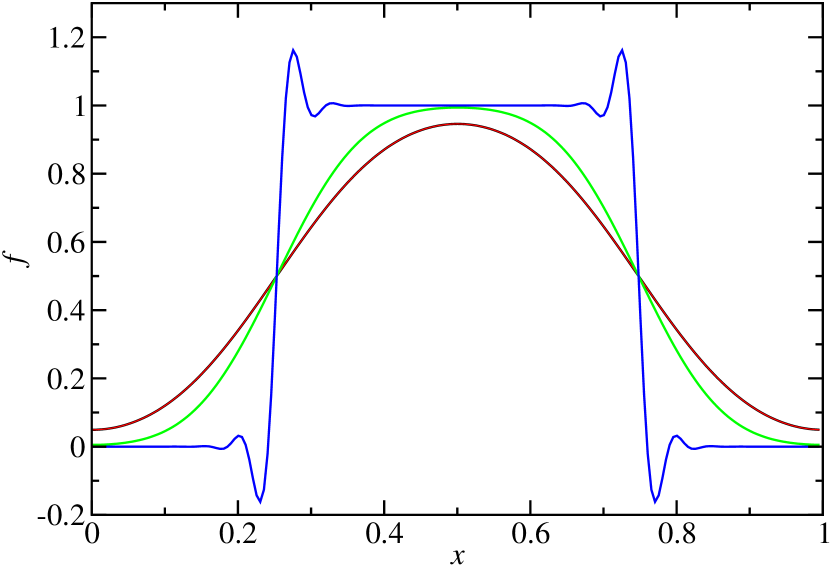
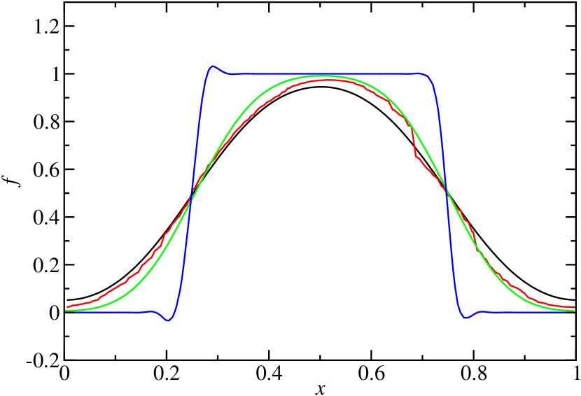
Figure 1: Results for the moving top-hat function. Field after one traversal of the cell. Left: regular particle distribution, right: distorted. Black: $\delta$ projection, red: FLIP, green: mass-$\delta$, blue: full mass.

method	$E_{1}$	$E_{2}$	$L_{2}$
$\delta$	$0$	$-29\%$	$35\%$
FLIP	$0$	$-25\%$	$35\%$
mass-$\delta$	$0$	$-21\%$	$29\%$
full mass	$0$	$0.85\%$	$10\%$

method	$E_{1}$	$E_{2}$	$L_{2}$
$\delta$	$-0.24\%$	$-29\%$	$35\%$
FLIP	$0$	$-25\%$	$35\%$
mass-$\delta$	$0.7\%$	$-20\%$	$29\%$
full mass	$-0.7\%$	$-4\%$	$12\%$

Table 2: Results for 1D spacing. Left table: regular, right: distorted

3.2 Zalesak’s disk

Let us consider a region with a colour field $\alpha$ that has a value of $1$ for points inside a domain and $0$ for points outside and which is simply advected:

$$\frac{dA}{dt}=0\qquad\frac{d\mathbf{r}}{dt}=u.$$ (22)

The domain is a circle with a slot. The circle’s radius is given a value of $R=0.5$, while the slot was a width of $1/6$, and a height of $5/6$. The simulation box is a $(-1.5,1.5)\times(-1.5,1.5)$ square, and the number of nodes is set to $90\times 90$, so that the mesh spacing is $H=3/90=1/30$, the same value as in [13]. The time step is $\Delta t=0.01$, which corresponds to $\mathrm{Co}_{H}:=u(\Delta t)/H\approx 0.94$ for nodes on the rim of the disk.

The velocity field is a pure rotation:

$$u_{x} =-\omega y$$ (23)

$$u_{y} =\omega x,$$ (24)

where $\omega=2\pi/\tau$, and the period of rotation is set to $\tau=1$. Periodic boundary conditions are used in this simulation, but this fact is not really important since the only region that is actually moved is within a circle of radius $1.4$, within a simulation box of size $3\times 3$.

For the mesh, and also for the particles in the mass methods, we use linear FE functions, as in the previous 1D example. These are piece-wise affine functions: pyramids of height $1$ at the node, decreasing to $0$ at the neighbouring nodes. We employ the Delaunay triangulation in order to determine these functions. For all mass methods, a moving Delaunay triangulation must be maintained for the projection from the mesh to the particles. The calculation of the corresponding mass matrix, and its inversion, is only needed for the full mass method.

Again, it would make little sense to project from and onto the mesh at every time-step, but for benchmarking purposes. Results are given in Figure 2, showing contour plots for values between $0.49$ and $0.51$ of the $\alpha$ field on the mesh nodes. We include the initial contour, the contour after one revolution, $T=\tau$, and after two revolutions, $T=2\tau$.

On the top left contours are shown for the $\delta$ procedure, and at the top right, for the FLIP procedure. Both are seen to greatly smear out the initial slab. At the bottom left, the full-$\delta$ procedure is show. This time, some remains of the slab are seen after one revolution. Finally, the full mass projection produces quite good profiles even after two revolutions.

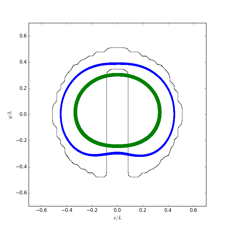
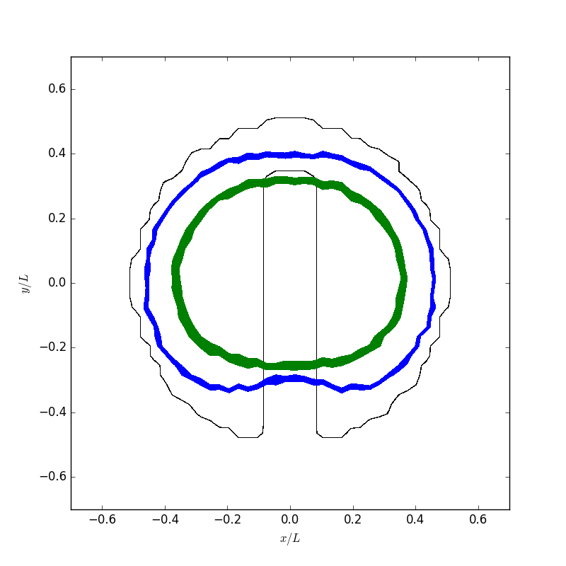
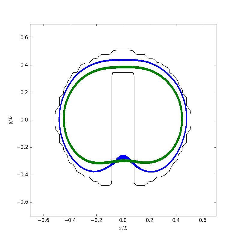
Figure 2: Results for the rotation of Zalesak’s disk. Isocontours for $\alpha\in(0.49,0.51)$. Initial field in black, after one rotation in blue, after two in green. Top left: $\delta$ method. Top right: FLIP. Bottom left: mass-$\delta$. Bottom right: full mass.

As in 1D, the good results of the full mass method maintaining the plateaus are accompanied by undershoots below $0$ and overshoots above $1$. In Figure 3 we show more detailed contours for the full mass procedure. The isocontour for $\alpha=0.5$ is shown again, but the $\alpha=0$ contour reveals a corona of slightly negative values, as low as $-0.05$ approximately. Values of $\alpha$ about $1.05$ are also seen in the inner regions.

Figure 3: Results for the rotation of Zalesak’s disk using the full mass method. Isocontours for $\alpha\in(-0.05,0,0.5,1,1.05)$ after two rotations.

We again employ the same error measures for our profiles. For the relative $L_{2}$ distance we introduce a refinement, by comparing the final profile and the one for a simulation in which the particle field is simply advected. This way we subtract out the errors due to time integration, by which particles’ trajectories are not exactly circles. These errors are quite small anyway.

method	$E_{1}$	$E_{2}$	$L_{2}$
$\delta$	$-0.5\%$	$-29\%$	$67\%$
FLIP	$0.14\%$	$-61\%$	$67\%$
mass-$\delta$	$-0.5$	$-50\%$	$61\%$
full mass	$0.5\%$	$-9\%$	$30\%$

Table 3: Results for the rotation of Zalesak’s disk.

3.3 Taylor-Green vortices

The Taylor-Green vortex sheet is an analytic solution to the Navier-Stokes equations for an incompressible Newtonian fluid:

$$\frac{d\mathbf{u}}{dt}=-\nabla p+\nu\nabla^{2}\mathbf{u}.$$ (25)

The solution, with a periodic length of $L$, is the velocity field

$$\mathbf{u}_{x} =f(t)\sin(kx)\cos(ky)$$ (26)

$$\mathbf{u}_{y} =-f(t)\cos(kx)\sin(ky),$$ (27)

where $k=2\pi/L$, and the time-dependent prefactor function is given by

$$f(t)=u_{0}\exp\left(-8\pi^{2}t^{*}/\mathrm{Re}\right).$$

The Reynolds number is defined as Re$:=u_{0}L/\nu$, and the dimensionless time is $t^{*}:=tu_{0}/L$. We set $u_{0}=1$, $L=1$, and $\nu=0.005$, thus setting a Reynolds number of Re=$200$.

For the numerical solution of the Navier-Stokes equation, a standard splitting approach is used [6]. The procedure is a simple mid-point time integration, as in Ref. [9]. All space derivatives are calculated on the mesh. As explained there, and in Ref. [13], even this integrator, with $\Delta t^{2}$ accuracy, will result in a $\Delta t$ overall accuracy. This is because the projection procedure causes a $\Delta t$ bottleneck in the calculation. A possible remedy, proposed in Ref. [9], is to include higher order basis functions. This idea is completely compatible with the ones put forward here, but for the sake of simplicity we will not discuss them.

In order to quantify the accuracy of the different methods, the relative $L_{2}$ distance between the velocity field obtained by simulation and its exact value is computed:

$$L_{2}:=\sqrt{\frac{\sum_{i=1}^{N}V_{i}\left|\mathbf{u}(\mathbf{r}_{i})-\mathbf{u}_{i}\right|^{2}}{\sum_{i=1}^{N}V_{i}|\mathbf{u}(\mathbf{r}_{i})|^{2}}},$$ (29)

where $\mathbf{u}(\mathbf{r}_{i})$ is the exact velocity field as in (26), evaluated on particle $i$ position. The same measure may be evaluated for mesh nodes, with very similar results.

This error is expected to start at a very low value and increase approximately linearly as the simulation proceeds. In order to compare between methods, in Fig. 4 the value of this error at $T^{*}=1$ is plotted. At this time, $f(T)=\exp(-8\pi^{2}/200)=0.67$, so that the velocity field should have decreased to about $67\%$ of its initial value.

The error for the velocity field (left subfigure) is seen to decrease with $\Delta t$. The interparticle and mesh spacing is decreased as $\Delta t$ does, in order to fix a Courant number of Co${}_{H}=0.5$ (the number of nodes and particles therefore increases quadratically). Like in Zalesak’s disk test, there are as many particles as nodes. The particles are created at the beginning of the simulation and moved according to the velocity field. As expected, the order of convergence of the error agrees with a $\Delta t^{1}$ power in all cases. However, results from the full mass procedure are much more accurate.

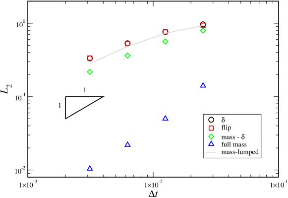
Figure 4: $L_{2}$ error of the velocity field at time $T^{*}=1$, versus time step $\Delta t$. Black circles: $\delta$ method, red squares: FLIP, green diamonds: mass-$\delta$, blue triangles: full mass. The triangle shows a $\Delta t^{1}$ power-law.

Despite its superior performance, the full mass is clearly more costly computationally than the alternatives. It therefore seems interesting to plot the error as a function of CPU time. A bad scaling as the number of nodes and particles is increased would make this procedure less appealing. However, Fig. 5 makes clear that the full mass procedure scales similarly to other procedures, with $L_{2}$ roughly proportional to $\Delta t^{1/2}$.

The CPU run times are clearly depend on the machine used, but a faster one, would likely make all simulations faster by a similar factor. This would result in a horizontal translation of all the curves in a logarithmic scale. Results do depend on the particular linear algebra algorithm used, details can be found in Appendix A.

One may therefore conclude from these observations that the higher computational cost of a full mass method will be compensated by its higher accuracy.

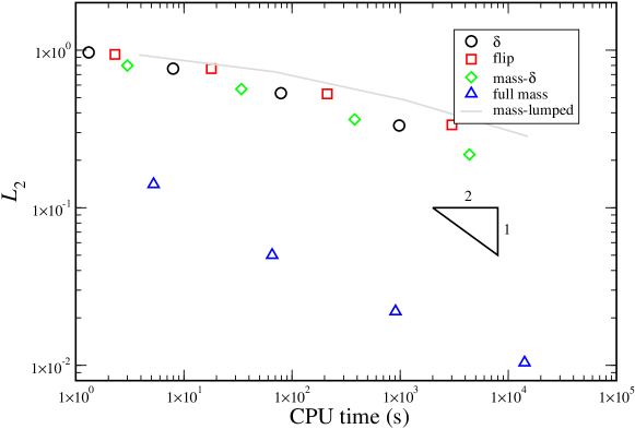
Figure 5: $L_{2}$ error of the velocity field at time $T^{*}=1$, versus CPU time in seconds Black circles: $\delta$ method, red squares: FLIP, green diamonds: mass-$\delta$, blue triangles: full mass. The triangle shows a $\Delta t^{1}$ power-law.

4 Conclusions

We have described several assignment, or projection, procedures by which field information may be transferred between particles and mesh. We have focused on four procedures: the simplest $\delta$ method, the FLIP method, the mass-$\delta$ method and the full mass method.

Each method is tested against several requirements: conservativity, which makes sure that the total integral of a field is not changed; stability, that ensures that the integral of the square of a field decreases upon projection; and preservation of information, which means that an assignment procedure, followed by interpolation, leaves the field values invariant.

We have tested the method in 1D and 2D advection problems. Conservativity is satisfied exactly by construction in the FLIP method, and rather well satisfied in the other cases. Stability is satisfied in all four methods, but the full mass method is seen to be superior in producing a smaller decrease. On the other hand, it also leads to higher over- and undershoots at sharp interfaces.

Finally, the full mass method is clearly superior in our CFD simulations of the Taylor-Green vortex sheet, where an approximate $10$-fold increase in accuracy is achieved for the same simulation clock time.

The final conclusion is that the full mass method should be seriously considered as an assignment procedure, despite its inherent higher computational complexity.

Appendix A Numerical methods

For all computational geometry procedures the CGAL 4.7 libraries [3] are used. In particular, the 2D Periodic Delaunay Triangulation package, overloading the vertex base to contain the relevant fields, and the face base to contain information relevant to the edges.

The Eigen 3.0 linear algebra libraries [12] are also employed. For the small linear algebra problem involved in the calculation of the $A$ coefficients, SVD is used, with automatic rank detection. For the large problems involved in the Galerkin procedure, the sparse matrix package is used. The linear systems are solved iteratively for pFEM, by the BiCGSTAB method. For projFEM a direct method is employed, with best results obtained using the CHOLMOD [4] routines of the suitesparse project (through Eigen wrappers for convenience, class CholmodSupernodalLLT). Slightly worse results are obtained with eigen’s build-in SimplicialLDLT class.

Our computations took place on a 4-core Pentium 4 machine with 16 Gb RAM. The code employed, named polyFEM, may be found in [8] under an open source license.

Appendix B Quadrature

As explained in the main text, the “mass” assignments involve integrals as in Equation (13).

In this work, the $A(\mathbf{r})$ is a piece-wise linear function, that connects the values of at the particles $A_{\mu}$. The fact that the locations of mesh nodes and particles do not match makes the integral somewhat cumbersome to evaluate. We have therefore implemented a simple quadrature rule. It is best visualized in 1D, see Figure 6. For the interval between node $i$ and $i+1$ function $A(x)$ is evaluated at $x_{i}$, $x_{i+1}$ and the position in between. The resulting three values are then fit to a parabola, whose overlap integral (functional scalar product) with $\phi_{i}$ is trivial to evaluate. As shown in the Figure, if no particles lie on the interval, this approximation is exact: the parabola will degenerate to a line in this case. If some particle lies in the interval the result will be, in general, an approximation. For each node $i$ there will be an additional integration from $i-1$ to $i$.

The same procedure is carried out in 2D, as also depicted in Figure 6. The view is from above, and for simplicity only 2D points are drawn, not functions. Function $A(\mathbf{r})$ is evaluated at the nodes of the triangle that connects node $i$ and two of its neighbours in the triangulation. In addition, it is also evaluated at the mid-points of each segment. With these six values, an interpolating quadratic function is found, whose overlap integral with $\phi_{i}$ is trivial. Again, if no particles happen to lie in the triangle the procedure is exact, but it is approximate if one or more particles do lie in the triangle. For each node $i$ integration must be performed over all its other incident triangles.

An equivalent procedure is applied in the inverse procedure of 20.

      

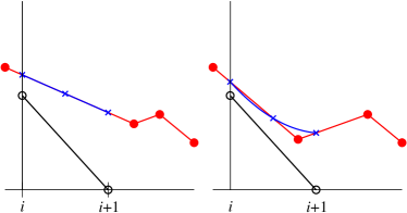
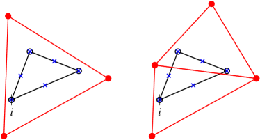
Figure 6: Illustration of the quadrature used in 1D (left two figures), and 2D (right two figures). Black empty circles: position of nodes. Red full circles: position of circles. Blue crosses: quadrature points. In 1D, $\phi_{i}(x)$ is shown as a black line, and $A(x)$ as a red line. The quadratic approximation to the latter is shown as a blue line.

References

- [1] A.A. Amsden. The particle-in-cell method for the calculation of the dynamics of compressible fluids. Technical Report LA-3466, Los Alamos Scientific Laboratory, 1966.
- [2] Robert Bridson. Fluid simulation for computer graphics. CRC Press, 2015.
- [3] CGAL Editorial Board. Cgal, Computational Geometry Algorithms Library. http://www.cgal.org.
- [4] Y Chen, T A Davis, W W Hager, and S Rajamanickam. Algorithm 887: Cholmod, supernodal sparse cholesky factorization and update/downdate. ACM Trans Math Software, 35(3), 2009.
- [5] IP Christiansen. Numerical simulation of hydrodynamics by the method of point vortices. Journal of Computational Physics, 13(3):363–379, 1973.
- [6] Ramon Codina. Pressure stability in fractional step finite element methods for incompressible flows. Journal of Computational Physics, 170(1):112–140, 2001.
- [7] Georges-Henri Cottet and Petros D Koumoutsakos. Vortex methods: theory and practice. Cambridge university press, 2000.
- [8] Daniel Duque. polyFEM 1.0. https://github.com/ddcampayo/polyFEM, 2016.
- [9] Daniel Duque and P Español. International journal for numerical methods in engineering. Quadratically consistent projection from particles to mesh, 2016.
- [10] Martha W Evans, Francis H Harlow, and Eleazer Bromberg. The particle-in-cell method for hydrodynamic calculations. Technical report, Los Alamos Scientific Laboratory, 1957.
- [11] M.W. Evans and F.H. Harlow. The particle-in-cell method for hydrodynamic calculations. Technical Report LA-2139, Los Alamos Scientific Laboratory, 1957.
- [12] Gaël Guennebaud, Benoît Jacob, et al. Eigen v3. http://eigen.tuxfamily.org, 2010.
- [13] Sergio Idelsohn, Eugenio Oñate, Norberto Nigro, Pablo Becker, and Juan Gimenez. Lagrangian versus Eulerian integration errors. Computer Methods in Applied Mechanics and Engineering, 293:191–206, 2015.
- [14] J Reddy. An Introduction to the Finite Element Method. McGraw-Hill Series in Mechanical Engineering. McGraw-Hill Education, 2005.