Lazifying Conditional Gradient Algorithms

Abstract

Conditional gradient algorithms (also often called Frank-Wolfe algorithms) are popular due to their simplicity of only requiring a linear optimization oracle and more recently they also gained significant traction for online learning. While simple in principle, in many cases the actual implementation of the linear optimization oracle is costly. We show a general method to lazify various conditional gradient algorithms, which in actual computations leads to several orders of magnitude of speedup in wall-clock time. This is achieved by using a faster separation oracle instead of a linear optimization oracle, relying only on few linear optimization oracle calls.

1 Introduction

Convex optimization is an important technique both from a theoretical and an applications perspective. Gradient descent based methods are widely used due to their simplicity and easy applicability to many real-world problems. We are interested in solving constraint convex optimization problems of the form

$$\min_{x\in P}f(x),$$ (1)

where $f$ is a smooth convex function and $P$ is a polytope, with access to $f$ being limited to first-order information, i.e., we can obtain $\nabla f(x)$ and $f(x)$ for a given $x\in P$ and access to $P$ via a linear minimization oracle, which returns $\operatorname{LP}_{P}(c)=\operatorname{argmin}_{x\in P}cx$ for a given linear objective $c$.

Algorithm 1 Frank-Wolfe Algorithm (Frank and Wolfe, 1956)

0:  smooth convex function $f$ with curvature $C$, start vertex $x_{1}\in P$, linear minimization oracle $\operatorname{LP}_{P}$

0:  points $x_{t}$ in $P$

1:  for $t=1$ to $T-1$ do

2:     $v_{t}\leftarrow\operatorname{LP}_{P}(\nabla f(x_{t}))$

3:     $x_{t+1}\leftarrow(1-\gamma_{t})x_{t}+\gamma_{t}v_{t}$ with $\gamma_{t}\coloneqq\frac{2}{t+2}$

4:  end for

When solving Problem (1) using gradient descent approaches in order to maintain feasibility, typically a projection step is required. This projection back into the feasible region $P$ is potentially computationally expensive, especially for complex feasible regions in very large dimensions. As such, projection-free methods gained a lot of attention recently, in particular the Frank-Wolfe algorithm (Frank and Wolfe, 1956) (also known as conditional gradient descent (Levitin and Polyak, 1966); see also (Jaggi, 2013) for an overview) and its online version (Hazan and Kale, 2012) due to their simplicity. We recall the basic Frank-Wolfe algorithm in Algorithm 1. These methods eschew the projection step and rather use a linear optimization oracle to stay within the feasible region. While convergence rates and regret bounds are often suboptimal, in many cases the gain due to only having to solve a single linear optimization problem over the feasible region in every iteration still leads to significant computational advantages (see e.g., (Hazan and Kale, 2012, Section 5)). This led to conditional gradient algorithms being used for e.g., online optimization and more generally machine learning. Also the property that these algorithms naturally generate sparse distributions over the extreme points of the feasible region is often helpful. Further increasing the relevance of these methods, it was shown recently that conditional gradient methods can also achieve linear convergence (see e.g., Garber and Hazan (2013); Lacoste-Julien and Jaggi (2015); Garber and Meshi (2016)) as well as that the number of total gradient evaluations can be reduced while maintaining the optimal number of oracle calls as shown in Lan and Zhou (2014).

Unfortunately, for complex feasible regions even solving the linear optimization problem might be time-consuming and as such the cost of solving the LP might be non-negligible. This could be the case, e.g., when linear optimization over the feasible region is a hard problem or when solving large-scale optimization or learning problems. As such it is natural to ask the following questions:

1. Does the linear optimization oracle have to be called in every iteration?

2. Does one need approximately optimal solutions for convergence?

3. Can one reuse information across iterations?

We will answer these questions in this work, showing that (i) the LP oracle is not required to be called in every iteration, (ii) much weaker guarantees are sufficient, and (iii) we can reuse information. To significantly reduce the cost of oracle calls while maintaining identical convergence rates up to small constant factors, we replace the linear optimization oracle by a (weak) separation oracle

Oracle 1 Weak Separation Oracle $\operatorname{LPsep}_{P}(c,x,\Phi,K)$

0:  linear objective $c\in\mathbb{R}^{n}$, point $x\in P$, accuracy $K\geq 1$, objective value $\Phi>0$;

0:  Either (1) vertex $y\in P$ with $c(x-y)>\Phi/K$ (2) false: $c(x-z)\leq\Phi$ for all $z\in P$

(Oracle 1) which approximately solves a separation problem within a multiplicative factor and returns improving vertices. We stress that the weak separation oracle is significantly weaker than approximate minimization, which has been already considered in Jaggi (2013). In fact, there is no guarantee that the improving vertices returned by the oracle are near to the optimal solution to the linear minimization problem. It is this relaxation of dual bounds and approximate optimality that will provide a significant speedup as we will see later. However, if the oracle does not return an improving vertex (returns false), then this fact can be used to derive a reasonably small dual bound of the form: $f(x_{t})-f(x^{*})\leq\nabla f(x_{t})(x_{t}-x^{*})\leq\Phi_{t}$ for some $\Phi_{t}>0$. While the accuracy $K$ is presented here as a formal argument of the oracle, an oracle implementation might restrict to a fixed value $K>1$, which often makes implementation easier. We point out that the cases (1) and (2) potentially overlap if $K>1$. This is intentional and in this case it is unspecified which of the cases the oracle should choose (and it does not matter for the algorithms).

This new oracle encapsulates the smart use of the original linear optimization oracle, even though for some problems it could potentially be implemented directly without relying on a linear programming oracle. Concretely, a weak separation oracle can be realized by a single call to a linear optimization oracle and as such is no more complex than the original oracle. However it has two important advantages: it allows for caching and early termination. Caching refers to storing previous solutions, and first searching among them to satisfy the oracle’s separation condition. The underlying linear optimization oracle is called only, when none of the cached solutions satisfy the condition. Algorithm 2 formalizes this process. Early termination is the technique to stop the linear optimization algorithm before it finishes at an appropriate stage, when from its internal data a suitable oracle answer can be easily recovered; this is clearly an implementation dependent technique. The two techniques can be combined, e.g., Algorithm 2 could use an early terminating linear oracle or other implementation of the weak separation oracle in line 4.

Algorithm 2 $\operatorname{LPsep}_{P}(c,x,\Phi,K)$ via LP oracle

0:  linear objective $c\in\mathbb{R}^{n}$, point $x\in P$, accuracy $K\geq 1$, objective value $\Phi>0$;

0:  Either (1) vertex $y\in P$ with $c(x-y)>\Phi/K$ (2) false: $c(x-z)\leq\Phi$ for all $z\in P$

1:  if $y\in P$ cached with $c(x-y)>\Phi/K$ exists then

2:     return  $y$ {Cache call}

3:  else

4:     $y\leftarrow\operatorname{argmax}_{x\in P}cx$ {LP call}

5:     if $c(x-y)>\Phi/K$ then

6:        add $y$ to cache

7:        return  $y$

8:     else

9:        return  false

10:     end if

11:  end if

We call lazification the technique of replacing a linear programming oracle with a much weaker one, and we will demonstrate significant speedups in wall-clock performance (see e.g., Figure 25), while maintaining identical theoretical convergence rates.

To exemplify our approach we provide conditional gradient algorithms employing the weak separation oracle for the standard Frank-Wolfe algorithm as well as the variants in (Hazan and Kale, 2012; Garber and Meshi, 2016; Garber and Hazan, 2013), which have been chosen due to requiring modified convergence arguments that go beyond those required for the vanilla Frank-Wolfe algorithm. Complementing the theoretical analysis we report computational results demonstrating effectiveness of our approach via a significant reduction in wall-clock time compared to their linear optimization counterparts.

Related Work

There has been extensive work on Frank-Wolfe algorithms and conditional gradient algorithms, so we will restrict to review work most closely related to ours. The Frank-Wolfe algorithm was originally introduced in (Frank and Wolfe, 1956) (also known as conditional gradient descent (Levitin and Polyak, 1966) and has been intensely studied in particular in terms of achieving stronger convergence guarantees as well as affine-invariant versions. We demonstrate our approach for the vanilla Frank-Wolfe algorithm (Frank and Wolfe, 1956) (see also (Jaggi, 2013)) as an introductory example. We then consider more complicated variants that require non-trivial changes to the respective convergence proofs to demonstrate the versatility of our approach. This includes the linearly convergent variant via local linear optimization (Garber and Hazan, 2013) as well as the pairwise conditional gradient variant of Garber and Meshi (2016), which is especially efficient in terms of implementation. However, our technique also applies to the Away-Step Frank-Wolfe algorithm, the Fully-Corrective Frank-Wolfe algorithm, the Pairwise Conditional Gradient algorithm, as well as the Block-Coordinate Frank-Wolfe algorithm. Recently, in Freund and Grigas (2016) guarantees for arbitrary step-size rules were provided and an analogous analysis can be also performed for our approach. On the other hand, the analysis of the inexact variants, e.g., with approximate linear minimization does not apply to our case as our oracle is significantly weaker than approximate minimization as pointed out earlier. For more information, we refer the interested reader to the excellent overview in (Jaggi, 2013) for Frank-Wolfe methods in general as well as Lacoste-Julien and Jaggi (2015) for an overview with respect to global linear convergence.

It was also recently shown in Hazan and Kale (2012) that the Frank-Wolfe algorithm can be adjusted to the online learning setting and in this work we provide a lazy version of this algorithm. Combinatorial convex online optimization has been investigated in a long line of work (see e.g., (Kalai and Vempala, 2005; Audibert et al., 2013; Neu and Bartók, 2013)). It is important to note that our regret bounds hold in the structured online learning setting, i.e., our bounds depend on the $\ell_{1}$-diameter or sparsity of the polytope, rather than its ambient dimension for arbitrary convex functions (see e.g., (Cohen and Hazan, 2015; Gupta et al., 2016)). We refer the interested reader to (Hazan, 2016) for an extensive overview.

A key component of the new oracle is the ability to cache and reuse old solutions, which accounts for the majority of the observed speed up. The idea of caching of oracle calls was already explored in various other contexts such as cutting plane methods (see e.g., Joachims et al. (2009)) as well as the Block-Coordinate Frank-Wolfe algorithm in Shah et al. (2015); Osokin et al. (2016). Our lazification approach (which uses caching) is however much more lazy, requiring no multiplicative approximation guarantee; see (Osokin et al., 2016, Proof of Theorem 3. Appendix F) and Lacoste-Julien et al. (2013) for comparison to our setup.

Contribution

The main technical contribution of this paper is a new approach, whereby instead of finding the optimal solution, the oracle is used only to find a good enough solution or a certificate that such a solution does not exist, both ensuring the desired convergence rate of the conditional gradient algorithms.

Our contribution can be summarized as follows:

1. Lazifying approach. We provide a general method to lazify conditional gradient algorithms. For this we replace the linear optimization oracle with a weak separation oracle, which allows us to reuse feasible solutions from previous oracle calls, so that in many cases the oracle call can be skipped. In fact, once a simple representation of the underlying feasible region is learned no further oracle calls are needed. We also demonstrate how parameter-free variants can be obtained.

2. Lazified conditional gradient algorithms. We exemplify our approach by providing lazy versions of the vanilla Frank-Wolfe algorithm as well as of the conditional gradient methods in (Hazan and Kale, 2012; Garber and Hazan, 2013; Garber and Meshi, 2016).

3. Weak separation through augmentation. We show in the case of 0/1 polytopes how to implement a weak separation oracle with at most $k$ calls to an augmentation oracle that on input $c\in\mathbb{R}^{n}$ and $x\in P$ provides either an improving solution $\overline{x}\in P$ with $c\overline{x}<cx$ or ensures optimality, where $k$ denotes the $\ell_{1}$-diameter of $P$. This is useful when the solution space is sparse.

4. Computational experiments. We demonstrate computational superiority by extensive comparisons of the weak separation based versions with their original versions. In all cases we report significant speedups in wall-clock time often of several orders of magnitude.

It is important to note that in all cases, we inherit the same requirements, assumptions, and properties of the baseline algorithm that we lazify. This includes applicable function classes, norm requirements, as well as smoothness and (strong) convexity requirements. We also maintain identical convergence rates up to (small) constant factors.

A previous version of this work appeared as extended abstract in Braun et al. (2017); this version has been significantly revised over the conference version including a representative subset of more extensive computational results, full proofs for all described variants, as well as a variant that uses an augmentation oracle instead of linear optimization oracle (see Section 6).

Outline

We briefly recall notation and notions in Section 2 and consider conditional gradient algorithms in Section 3. In Section 4 we consider parameter-free variants of the proposed algorithms, and in Section 5 we examine online versions. Finally, in Section 6 we show a realization of a weak separation oracle with an even weaker oracle in the case of combinatorial problem and we provide extensive computational results in Section 7.

2 Preliminaries

Let $\lVert\cdot\rVert$ be an arbitrary norm on $\mathbb{R}^{n}$, and let $\mathinner{\lVert\mathord{\cdot}\rVert^{*}}$ denote the dual norm of $\lVert\mathord{\cdot}\rVert$. A function $f$ is $L$-Lipschitz if $\lvert f(y)-f(x)\rvert\leq L\lVert y-x\rVert$ for all $x,y\in\operatorname{dom}f$. A convex function $f$ is smooth with curvature at most $C$ if

$$f(\gamma y+(1-\gamma)x)\leq f(x)+\gamma\nabla f(x)(y-x)+C\gamma^{2}/2$$

for all $x,y\in\operatorname{dom}f$ and $0\leq\gamma\leq 1$. A function $f$ is $S$-strongly convex if

$$f(y)-f(x)\geq\nabla f(x)(y-x)+\frac{S}{2}\lVert y-x\rVert^{2}$$

for all $x,y\in\operatorname{dom}f$. Unless stated otherwise Lipschitz continuity and strong convexity will be measured in the norm $\lVert\cdot\rVert$. Moreover, let $\mathbb{B}_{r}\left({x}\right)\coloneqq\{y\mid\lVert x-y\rVert\leq r\}$ be the ball around $x$ with radius $r$ with respect to $\lVert.\rVert$. In the following, $P$ will denote the feasible region, a polytope and the vertices of $P$ will be denoted by $v_{1},\dots,v_{N}$.

3 Lazy Conditional Gradient

We start with the most basic Frank-Wolfe algorithm as a simple example for lazifying by means of a weak separation oracle. We then lazify more complex Frank-Wolfe algorithms in Garber and Hazan (2013) and Garber and Meshi (2016). Throughout this section $\lVert\cdot\rVert$ denotes the $\ell_{2}$-norm.

3.1 Lazy Conditional Gradient: a basic example

We start with lazifying the original Frank-Wolfe algorithm (arguably the simplest Conditional Gradient algorithm), adapting the baseline argument from (Jaggi, 2013, Theorem 1). While the vanilla version has suboptimal convergence rate $O(1/T)$, its simplicity makes it an illustrative example of the main idea of lazification. The lazy algorithm (Algorithm 3) maintains an upper bound $\Phi_{t}$ on the convergence rate, guiding its eagerness for progress when searching for an improving vertex $v_{t}$. If the weak separation oracle provides an improving vertex $v_{t}$ we refer to this as a positive call and if the oracle claims there are no improving vertices we call it a negative call.

Algorithm 3 Lazy Conditional Gradient

0:  smooth convex function $f$ with curvature $C$, start vertex $x_{1}\in P$, weak linear separation oracle $\operatorname{LPsep}_{P}$, accuracy $K\geq 1$, step sizes $\gamma_{t}$, initial upper bound $\Phi_{0}$

0:  points $x_{t}$ in $P$

1:  for $t=1$ to $T-1$ do

2:      $\Phi_{t}\leftarrow\frac{\Phi_{t-1}+\frac{C\gamma_{t}^{2}}{2}}{1+\frac{\gamma_{t}}{K}}$

3:      $v_{t}\leftarrow\operatorname{LPsep}_{P}(\nabla f(x_{t}),x_{t},\Phi_{t},K)$

4:     if $v_{t}=\textbf{false}{}$ then

5:         $x_{t+1}\leftarrow x_{t}$

6:     else

7:         $x_{t+1}\leftarrow(1-\gamma_{t})x_{t}+\gamma_{t}v_{t}$

8:     end if

9:  end for

The step size $\gamma_{t}$ is chosen to (approximately) minimize $\Phi_{t}$ in Line 2; roughly $\Phi_{t-1}/KC$.

Theorem 3.1.

Assume $f$ is convex and smooth with curvature $C$. Then Algorithm 3 with $\gamma_{t}=\frac{2(K^{2}+1)}{K(t+K^{2}+2)}$ and $f(x_{1})-f(x^{*})\leq\Phi_{0}$ has convergence rate

$$f(x_{t})-f(x^{*})\leq\frac{2\max\{C,\Phi_{0}\}(K^{2}+1)}{t+K^{2}+2},$$ (2)

where $x^{*}$ is a minimum point of $f$ over $P$.

Proof.

We prove by induction that

$$f(x_{t})-f(x^{*})\leq\Phi_{t-1}.$$

The claim is clear for $t=1$ by the choice of $\Phi_{0}$. Assuming the claim is true for $t$, we prove it for $t+1$. We distinguish two cases depending on the return value of the weak separation oracle in Line 3.

In case of a positive call, i.e., when the oracle returns an improving solution $v_{t}$, then $\nabla f(x_{t})(x_{t}-v_{t})\geq\Phi_{t}/K$, which is used in the second inequality below. The first inequality follows by smoothness of $f$, and the second inequality by the induction hypothesis and the fact that $v_{t}$ is an improving solution:

$$f(x_{t+1})-f(x^{*}) \leq\underbrace{f(x_{t})-f(x^{*})}_{\leq\Phi_{t-1}}+\gamma_{t}\underbrace{\nabla f(x_{t})(v_{t}-x_{t})}_{\leq-\Phi_{t}/K}+\frac{C\gamma_{t}^{2}}{2}$$

$$\leq\Phi_{t-1}-\gamma_{t}\frac{\Phi_{t}}{K}+\frac{C\gamma_{t}^{2}}{2}$$

$$=\Phi_{t},$$

In case of a negative call, i.e., when the oracle returns no improving solution, then in particular $\nabla f(x_{t})(x_{t}-x^{*})\leq\Phi_{t}$, hence by Line 5

$$f(x_{t+1})-f(x^{*})=f(x_{t})-f(x^{*})\leq\nabla f(x_{t})(x_{t}-x^{*})\leq\Phi_{t}.$$ (3)

Finally, using the specific values of $\gamma_{t}$ we prove the upper bound

$$\Phi_{t-1}\leq\frac{2\max\{C,\Phi_{0}\}(K^{2}+1)}{t+K^{2}+2}$$ (4)

by induction on $t$. The claim is obvious for $t=1$. The induction step is an easy computation relying on the definition of $\Phi_{t}$ on Line 2:

$$\Phi_{t}=\frac{\Phi_{t-1}+\frac{C\gamma_{t}^{2}}{2}}{1+\frac{\gamma_{t}}{K}}\leq\frac{\frac{2\max\{C,\Phi_{0}\}(K^{2}+1)}{t+K^{2}+2}+\frac{\max\{C,\Phi_{0}\}\gamma_{t}^{2}}{2}}{1+\frac{\gamma_{t}}{K}}\leq\frac{2\max\{C,\Phi_{0}\}(K^{2}+1)}{t+K^{2}+3}.$$ (5)

Here the last inequality follows from the concrete value of $\gamma_{t}$. ∎

Note that by design, the algorithm converges at the worst-case rate that we postulate due to the negative calls when it does not move. Clearly, this is highly undesirable, therefore the algorithm should be understood as the textbook variant of lazy conditional gradient. We will present an improved, parameter-free variant of Algorithm 3 in Section 4 that converges at the best possible rate that the non-lazy variant would achieve (up to a small constant factor).

3.2 Lazy Pairwise Conditional Gradient

In this section we provide a lazy variant (Algorithm 4) of the Pairwise Conditional Gradient algorithm from Garber and Meshi (2016), using separation instead of linear optimization. We make identical assumptions: the feasible region is a $0/1$ polytope, i.e., all vertices of $P$ have only $0/1$ entries, and moreover it is given in the form $P=\{x\in\mathbb{R}^{n}\mid 0\leq x\leq\mathbb{1},Ax=b\}$, where $\mathbb{1}$ denotes the all-one vector.

Algorithm 4 Lazy Pairwise Conditional Gradient (LPCG)

0:  polytope $P$, smooth and $S$-strongly convex function $f$ with curvature $C$, accuracy $K\geq 1$, non-increasing step-sizes $\eta_{t}$, eagerness $\Delta_{t}$

0:  points $x_{t}$

1:  $x_{1}\in P$ arbitrary and $\Phi_{0}\geq f(x_{1})-f(x^{*})$

2:  for $t=1,\dots,T$ do

3:     $\widetilde{\nabla}f(x_{t})_{i}\coloneqq\begin{cases}\nabla f(x_{t})_{i}&\text{if }x_{t,i}>0\\ -\infty&\text{if }x_{t,i}=0\end{cases}$

4:     $\Phi_{t}\leftarrow\frac{2\Phi_{t-1}+\eta_{t}^{2}C}{2+\frac{\eta_{t}}{K\Delta_{t}}}$

5:      $c_{t}\leftarrow\left(\nabla f(x_{t}),-\widetilde{\nabla}f(x_{t})\right)$

6:      $(v_{t}^{+},v_{t}^{-})\leftarrow\operatorname{LPsep}_{P\times P}\left(c_{t},\,(x_{t},x_{t}),\,\frac{\Phi_{t}}{\Delta_{t}},\,K\right)$

7:     if $(v_{t}^{+},v_{t}^{-})=\textbf{false}{}$ then

8:         $x_{t+1}\leftarrow x_{t}$

9:     else

10:         $\tilde{\eta}_{t}\leftarrow\max\{2^{-\delta}\mid\delta\in\mathbb{Z}_{\geq 0},\ 2^{-\delta}\leq\eta_{t}\}$

11:         $x_{t+1}\leftarrow x_{t}+\tilde{\eta}_{t}(v_{t}^{+}-v_{t}^{-})$

12:     end if

13:  end for

Observe that Algorithm 4 calls the linear separation oracle $\operatorname{LPsep}$ on the cartesian product of $P$ with itself. Choosing the objective function as in Line 5 allows us to simultaneously find an improving direction and an away-step direction.

Let $\operatorname{card}{x}$ denote the number of non-zero entries of the vector $x$.

Theorem 3.2.

Let $x^{*}$ be a minimum point of $f$ in $P$, and $\Phi_{0}$ an upper bound of $f(x_{1})-f(x^{*})$. Furthermore, let $\operatorname{card}(x^{*})\leq\alpha$, $M_{1}\coloneqq\sqrt{\frac{S}{8\alpha}}$, $\kappa\coloneqq\min\left\{\frac{M_{1}}{KC},1/\sqrt{\Phi_{0}}\right\}$, $\eta_{t}\coloneqq\kappa\sqrt{\Phi_{t-1}}$ and $\Delta_{t}\coloneqq\sqrt{\frac{2\alpha\Phi_{t-1}}{S}}$, then Algorithm 4 has convergence rate

$$f(x_{t+1})-f(x^{*})\leq\Phi_{t}\leq\Phi_{0}\left(\frac{1+B}{1+2B}\right)^{t},$$

where $B\coloneqq\kappa\cdot\frac{M_{1}}{2K}$.

We recall a technical lemma for the proof.

Lemma 3.3 ((Garber and Meshi, 2016, Lemma 2)).

Let $x,y\in P$. Then $x$ is a liner combination $x=\sum_{i=1}^{k}\lambda_{i}v_{i}$ of some vertices $v_{i}$ of $P$ (in particular, $\sum_{i=1}^{k}\lambda_{i}=1$) with $x-y=\sum_{i=1}^{k}\gamma_{i}(v_{i}-z)$ for some $0\leq\gamma_{i}\leq\lambda_{i}$ and $z\in P$ such that $\sum_{i=1}^{k}\gamma_{i}\leq\sqrt{\operatorname{card}(y)}\lVert x-y\rVert$.

Proof of Theorem 3.2.

The feasibility of the iterates $x_{t}$ is ensured by Line 10 and the monotonicity of the sequence $\{\eta_{t}\}_{t\geq 1}$ with the same argument as in (Garber and Meshi, 2016, Lemma 1 and Observation 2).

We first show by induction that

$$f(x_{t+1})-f(x^{*})\leq\Phi_{t}.$$

For $t=0$ we have $\Phi_{0}\geq f(x_{1})-f(x^{*})$. Now assume the statement for some $t\geq 0$. In case of a negative call (Line 8), we use the guarantee of Oracle 1 to get

$$c_{t}[(x_{t},x_{t})-(z_{1},z_{2})]\leq\frac{\Phi_{t}}{\Delta_{t}}$$

for all $z_{1},z_{2}\in P$, which is equivalent to (as $c_{t}(x_{t},x_{t})=0$)

$$\widetilde{\nabla}f(x_{t})z_{2}-\nabla f(x_{t})z_{1}\leq\frac{\Phi_{t}}{\Delta_{t}}$$

and therefore

$$\nabla f(x_{t})(\tilde{z}_{2}-z_{1})\leq\frac{\Phi_{t}}{\Delta_{t}},$$ (6)

for all $\tilde{z}_{2},z_{1}\in P$ with $\operatorname{supp}(\tilde{z}_{2})\subseteq\operatorname{supp}(x_{t})$, where $\operatorname{supp}(x)$ denotes the set of non-zero coordinates of $x$. We use Lemma 3.3 for the decompositions $x_{t}=\sum_{i=1}^{k}\lambda_{i}v_{i}$ and $x_{t}-x^{*}=\sum_{i=1}^{k}\gamma_{i}(v_{i}-z)$ with $0\leq\gamma_{i}\leq\lambda_{i}$, $z\in P$ and

$$\sum_{i=1}^{k}\gamma_{i}\leq\sqrt{\operatorname{card}(x^{*})}\lVert x_{t}-x^{*}\rVert\leq\sqrt{\frac{2\operatorname{card}(x^{*})\Phi_{t-1}}{S}}\leq\Delta_{t},$$

using the induction hypothesis and strong convexity in the second inequality. Then

$$f(x_{t+1})-f(x^{*})=f(x_{t})-f(x^{*})\leq\nabla f(x_{t})(x_{t}-x^{*})=\sum_{i=1}^{k}\gamma_{i}\cdot\underbrace{\nabla f(x_{t})(v_{i}-z)}_{\leq\Phi_{t}/\Delta_{t}}\leq\Phi_{t},$$

where we used Equation (6) for the last inequality.

In case of a positive call (Lines 10 and 11) we get, using first smoothness of $f$, then $\eta_{t}/2<\tilde{\eta_{t}}\leq\eta_{t}$ and $\nabla f(x_{t})(v_{t}^{+}-v_{t}^{-})\leq-\Phi_{t}/(K\Delta_{t})$, and finally the definition of $\Phi_{t}$:

$$f(x_{t+1})-f(x^{*}) =f(x_{t})-f(x^{*})+f(x_{t}+\tilde{\eta_{t}}(v_{t}^{+}-v_{t}^{-}))-f(x_{t})$$

$$\leq\Phi_{t-1}+\tilde{\eta}_{t}\nabla f(x_{t})(v_{t}^{+}-v_{t}^{-})+\frac{\tilde{\eta}_{t}^{2}C}{2}$$

$$\leq\Phi_{t-1}-\frac{\eta_{t}}{2}\cdot\frac{\Phi_{t}}{K\Delta_{t}}+\frac{\eta_{t}^{2}C}{2}=\Phi_{t}.$$

Plugging in the values of $\eta_{t}$ and $\Delta_{t}$ to the definition of $\Phi_{t}$ gives the desired bound.

$$\Phi_{t}=\frac{2\Phi_{t-1}+\eta_{t}^{2}C}{2+\frac{\eta_{t}}{K\Delta_{t}}}=\Phi_{t-1}\frac{1+\kappa^{2}C/2}{1+\kappa M_{1}/K}\leq\Phi_{t-1}\frac{1+B}{1+2B}\leq\Phi_{0}\left(\frac{1+B}{1+2B}\right)^{t}.\qed$$

3.3 Lazy Local Conditional Gradient

In this section we provide a lazy version (Algorithm 5) of the conditional gradient algorithm from Garber and Hazan (2013). Let $P\subseteq\mathbb{R}^{n}$ be any polytope, $D$ denote an upper bound on the $\ell_{2}$-diameter of $P$, and $\mu\geq 1$ be an affine invariant parameter of $P$ satisfying Lemma 3.4 below, see (Garber and Hazan, 2013, Section 2) for a possible definition. As the algorithm is not affine invariant by nature, we need a non-invariant version of smoothness: Recall that a convex function $f$ is $\beta$-smooth if

$$f(y)-f(x)\leq\nabla f(x)(y-x)+\beta\lVert y-x\rVert^{2}/2.$$

Algorithm 5 Lazy Local Conditional Gradient (LLCG)

0:  feasible polytope $P$, $\beta$-smooth and $S$-strongly convex function $f$, parameters $K$, $S$, $\beta$, $\mu$; diameter $D$

0:  points $x_{t}$

1:  $x_{1}\in P$ arbitrary and $\Phi_{0}\geq f(x_{1})-f(x^{*})$

2:  $\alpha\leftarrow\frac{S}{2K\beta n\mu^{2}}$

3:  for $t=1,\dots,T$ do

4:     $r_{t}\leftarrow\sqrt{\frac{2\Phi_{t-1}}{S}}$

5:     $\Phi_{t}\leftarrow\frac{\Phi_{t-1}+\frac{\beta}{2}\alpha^{2}\min\{n\mu^{2}r_{t}^{2},D^{2}\}}{1+\alpha/K}$

6:     $p_{t}\leftarrow\operatorname{LLPsep}_{P}\left(\nabla f(x_{t}),x_{t},r_{t},\Phi_{t},K\right)$

7:     if $p_{t}=\textbf{false}{}$ then

8:        $x_{t+1}\leftarrow x_{t}$

9:     else

10:         $x_{t+1}\leftarrow x_{t}+\alpha(p_{t}-x_{t})$

11:     end if

12:  end for

As an intermediary step, we first implement a local weak separation oracle in Algorithm 6, a local version of Oracle 1, which finds improving points only in a small neighbourhood of the original point, analogously to the local linear optimization oracle in Garber and Hazan (2013). To this end, we recall a technical lemma from Garber and Hazan (2013).

Algorithm 6 Weak Local Separation $\operatorname{LLPsep}_{P}(c,x,r,\Phi,K)$

0:  polytope $P$ together with invariant $\mu$, linear objective $c\in\mathbb{R}^{n}$, point $x\in P$, radius $r>0$, objective value $\Phi>0$, accuracy $K\geq 1$

0:  Either (1) $y\in P$with $\lVert x-y\rVert\leq\sqrt{n}\mu r$ and $c(x-y)>\Phi/K$ (2) false: $c(x-z)\leq\Phi$ for all $z\in P\cap\mathbb{B}_{r}\left({x}\right)$

1:  $\Delta\leftarrow\min\left\{\frac{\sqrt{n}\mu}{D}r,1\right\}$

2:  Decompose $x$: $x=\sum_{j=1}^{M}\lambda_{j}v_{j}$,  $\lambda_{j}>0$, $\sum_{j}\lambda_{j}=1$.

3:  Sort vertices: $i_{1},\dots,i_{M}$  $cv_{i_{1}}\geq\dots\geq cv_{i_{M}}$.

4:  $k\leftarrow\min\{k:\sum_{j=1}^{k}\lambda_{i_{j}}\geq\Delta\}$

5:  $p_{-}\leftarrow\sum_{j=1}^{k-1}\lambda_{i_{j}}v_{i_{j}}+\left(\Delta-\sum_{j=1}^{k-1}\lambda_{i_{j}}\right)v_{i_{k}}$

6:  $v^{*}\leftarrow\operatorname{LPsep}_{P}\left(c,\frac{p_{-}}{\Delta},\frac{\Phi}{\Delta}\right)$

7:  if $v^{*}=\textbf{false}{}$ then

8:     return   false

9:  else

10:     return   $y\leftarrow x-p_{-}+\Delta v^{*}$

11:  end if

Lemma 3.4.

(Garber and Hazan, 2013, Lemma 7) Let $P\subseteq\mathbb{R}^{n}$ be a polytope and $v_{1},\dots,v_{N}$ be its vertices. Let $x,y\in P$ and $x=\sum_{i=1}^{N}\lambda_{i}v_{i}$ a convex combination of the vertices of $P$. Then there are numbers $0\leq\gamma_{i}\leq\lambda_{i}$ and $z\in P$ satisfying

$$x-y =\sum_{i\in[N]}\gamma_{i}(z-v_{i})$$ (7)

$$\sum_{i\in[N]}\gamma_{i} \leq\frac{\sqrt{n}\mu}{D}\lVert x-y\rVert.$$ (8)

Now we prove the correctness of the weak local separation algorithm.

Lemma 3.5.

Algorithm 6 is correct. In particular $\operatorname{LLPsep}_{P}(c,x,r,\Phi,K)$

1. returns either an $y\in P$ with $\lVert x-y\rVert\leq\sqrt{n}\mu r$ and $c(x-y)\geq\Phi/K$,

2. or returns false, and then $c(x-z)\leq\Phi$ for all $z\in P\cap\mathbb{B}_{r}\left({x}\right)$.

Proof.

We first consider the case when the algorithm exits in Line 10. Observe that $y\in P$ since $y$ is a convex combination of vertices of by construction: $y=\sum_{j=1}^{M}(\lambda_{i_{j}}-\gamma_{j})v_{i_{j}}+\Delta v^{*}$ with $\Delta=\sum_{j=1}^{M}\gamma_{j}\leq\frac{\sqrt{n}\mu}{D}r$, where $\gamma_{j}=\lambda_{i_{j}}$ for $j<k$, and $\gamma_{k}=\Delta-\sum_{j=1}^{k-1}\lambda_{i_{j}}$, and $\gamma_{j}=0$ for $j>k$. Therefore

$$\lVert x-y\rVert=\left\lVert\sum_{j=1}^{M}\gamma_{j}(v_{i_{j}}-v^{*})\right\rVert\leq\sum_{j=1}^{M}\gamma_{j}\lVert v_{i_{j}}-v^{*}\rVert\leq\sqrt{n}\mu r.$$

Finally using the guarantee of $\operatorname{LPsep}_{P}$ we get

$$c(x-y)=\Delta c\left(\frac{p_{-}}{\Delta}-v^{*}\right)\geq\frac{\Phi}{K}.$$

If the algorithm exits in Line 8, we use Lemma 3.4 to decompose any $y\in P\cap\mathbb{B}_{r}\left({x}\right)$:

$$x-y=\sum_{i=1}^{M}\gamma_{i}(v_{i}-z),$$

with $z\in P$ and $\sum_{i=1}^{M}\gamma_{i}\leq\frac{\sqrt{n}\mu}{D}\lVert x-y\rVert\leq\Delta$. Since $\sum_{i=1}^{M}\lambda_{i}=1\geq\Delta$, there are numbers $\gamma_{i}\leq\eta_{i}^{-}\leq\lambda_{i}$ with $\sum_{i=1}^{M}\eta_{i}^{-}=\Delta$. Let

$$\tilde{p}_{-} \coloneqq\sum_{i=1}^{M}\eta_{i}^{-}v_{i},$$ (9)

$$\tilde{p}_{+} \coloneqq y-x+\tilde{p}_{-}=\sum_{i=1}^{M}(\eta_{i}^{-}-\gamma_{i})v_{i}+\sum_{i=1}^{M}\gamma_{i}z,$$ (10)

so that $\tilde{p}_{+}/\Delta\in P$. To bound the function value we first observe that the choice of $p_{-}$ in the algorithm assures that $cu\leq cp_{-}$ for all $u=\sum_{i=1}^{M}\eta_{i}v_{i}$ with $\sum_{i=1}^{M}\eta_{i}=\Delta$ and all $0\leq\eta_{i}\leq\lambda_{i}$. In particular, $c\tilde{p}_{-}\leq cp_{-}$. The function value of the positive part $\tilde{p}_{+}$ can be bounded with the guarantee of $\operatorname{LPsep}_{P}$:

$$c\left(\frac{p_{-}}{\Delta}-\frac{\tilde{p}_{+}}{\Delta}\right)\leq\frac{\Phi}{\Delta},$$

i.e., $c(p_{-}-\tilde{p}_{+})\leq\Phi$. Finally combining these bounds gives

$$c(x-y)=c\left(\tilde{p}_{-}-\tilde{p}_{+}\right)\leq c(p_{-}-\tilde{p}_{+})\leq\Phi$$

as desired. ∎

We are ready to examine the Conditional Gradient Algorithm based on $\operatorname{LLPsep}_{P}$:

Theorem 3.6.

Algorithm 5 converges with the following rate:

$$f(x_{t+1})-f(x^{*})\leq\Phi_{t}\leq\Phi_{0}\left(\frac{1+\alpha/(2K)}{1+\alpha/K}\right)^{t}.$$

Proof.

The proof is similar to the proof of Theorem 3.2. We prove this rate by induction. For $t=0$ the choice of $\Phi_{0}$ guarantees that $f(x_{1})-f(x^{*})\leq\Phi_{0}$. Now assume the theorem holds for $t\geq 0$. With strong convexity and the induction hypothesis we get

$$\lVert x_{t}-x^{*}\rVert^{2}\leq\frac{2}{S}(f(x_{t})-f(x^{*}))\leq\frac{2}{S}\Phi_{t-1}=r_{t}^{2},$$

i.e., $x^{*}\in P\cap\mathbb{B}_{r_{t}}\left({x_{t}}\right)$. In case of a negative call, i.e., when $p_{t}=\mathbf{false}$, then case (ii) of Lemma 3.5 applies:

$$f(x_{t+1})-f(x^{*})=f(x_{t})-f(x^{*})\leq\nabla f(x_{t})(x_{t}-x^{*})\leq\Phi_{t}.$$

In case of a positive call, i.e., when Line 10 is executed, we get the same inequality via:

$$f(x_{t+1})-f(x^{*}) \leq\Phi_{t-1}+\alpha\nabla f(x_{t})(p_{t}-x_{t})+\frac{\beta}{2}\alpha^{2}\lVert x_{t}-p_{t}\rVert^{2}$$

$$\leq\Phi_{t-1}-\alpha\frac{\Phi_{t}}{K}+\frac{\beta}{2}\alpha^{2}\min\{n\mu^{2}r_{t}^{2},D^{2}\}$$

$$=\Phi_{t}.$$

Therefore using the definition of $\alpha$ and $r_{t}$ we get the desired bound:

$$\Phi_{t}\leq\frac{\Phi_{t-1}+\frac{\beta}{2}\alpha^{2}r_{t}^{2}n\mu^{2}}{1+\alpha/K}=\Phi_{t-1}\left(\frac{1+\alpha/(2K)}{1+\alpha/K}\right)\leq\Phi_{0}\left(\frac{1+\alpha/(2K)}{1+\alpha/K}\right)^{t}.\qed$$

4 Parameter-free Conditional Gradient via Weak Separation

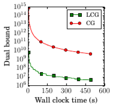
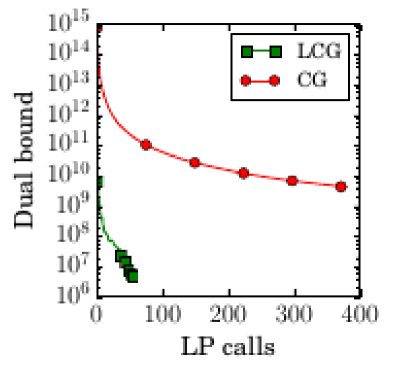
Figure 26: Performance on an instance of the video colocalization problem. We solve quadratic minimization over a flow polytope and report the achieved dual bound (or Wolfe-gap) over wall-clock time in seconds in logscale on the left and over the number of actual LP calls on the right. We used the parameter-free variant of the Lazy CG algorithm, which performs in both measures significantly better than the non-lazy counterpart. The performance difference is more prominent in the number of LP calls.

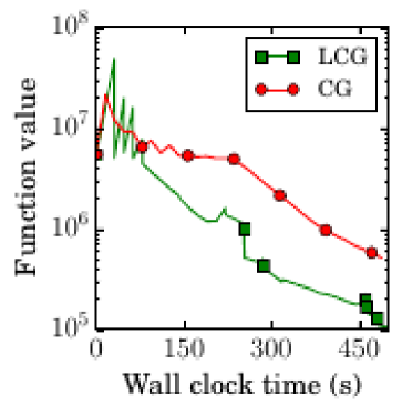
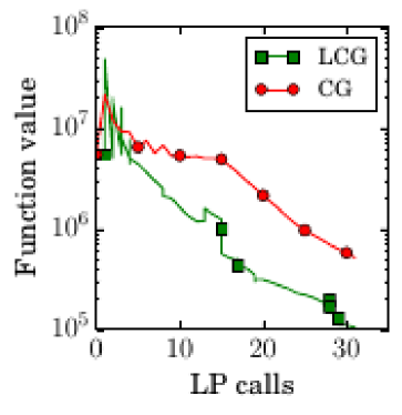
Figure 28: Performance on a matrix completion instance. More information about this problem can be found in the supplemental material (Section 7). The performance is reported as the objective function value over wall-clock time in seconds on the left and over LP calls on the right. In both measures after an initial phase the function value using LCG is much lower than with the non-lazy algorithm.

In this section we provide a parameter-free variant of the Lazy Frank-Wolfe Algorithm, which is inspired by Pokutta (2017) and which exhibits a very favorable behavior in computations; the same technique applies to all other variants from Section 3 as well. The idea is that instead of using predetermined values for progress parameters, like $\Phi_{t}$ and $\gamma_{t}$ in Algorithm 3, to optimize worst-case progress, the parameters are adjusted adaptively, using data encountered by the algorithm, and avoiding hard-to-estimate parameters, like the curvature $C$. In practice, this leads to faster convergence, as usual for adaptive methods, while the theoretical convergence rate is worse only by a small constant factor. See Figures 26 and 28 for a comparison and Section 7.1.1 for more experimental results.

The occasional halving of the $\Phi_{t}$ is reminiscent of an adaptive restart strategy, considering successive iterates with the same $\Phi_{t}$ as an epoch. It ensures that $\Phi_{t}$ is always at least half of the primal gap, while quickly reducing it if it is too large for the algorithm to make progress, and as such it represents a reasonable amount of expected progress throughout the whole run of the algorithm, not just at the initial iterates.

Algorithm 7 Parameter-free Lazy Conditional Gradient (LCG)

0:  smooth convex function $f$, start vertex $x_{1}\in P$, weak linear separation oracle $\operatorname{LPsep}_{P}$, accuracy $K\geq 1$

0:  points $x_{t}$ in $P$

1:   $\Phi_{0}\leftarrow\max_{x\in P}\nabla f(x_{1})(x_{1}-x)/2$ {Initial bound}

2:  for $t=1$ to $T-1$ do

3:      $v_{t}\leftarrow\operatorname{LPsep}_{P}(\nabla f(x_{t}),x_{t},\Phi_{t-1},K)$

4:     if $v_{t}=\textbf{false}{}$ then

5:        $x_{t+1}\leftarrow x_{t}$

6:         $\Phi_{t}\leftarrow\frac{\Phi_{t-1}}{2}$ {Update $\Phi$}

7:     else

8:        $\gamma_{t}\leftarrow\operatorname{argmin}_{0\leq\gamma\leq 1}f((1-\gamma)x_{t}+\gamma v_{t})$ {Line search}

9:        $x_{t+1}\leftarrow(1-\gamma_{t})x_{t}+\gamma_{t}v_{t}$ {Update iterate}

10:        $\Phi_{t}\leftarrow\Phi_{t-1}$

11:     end if

12:  end for

Remark 4.1 (Additional LP call for initial bound).

Note that Algorithm 7 finds a tight initial bound $\Phi_{0}$ with a single extra LP call. If this is undesired, this can be also done approximately as long as $\Phi_{0}$ is a valid upper bound, for example by means of binary search via the weak separation oracle.

Theorem 4.2.

Let $f$ be a smooth convex function with curvature $C$. Algorithm 7 converges at a rate proportional to $1/t$. In particular to achieve a bound $f(x_{t})-f(x^{*})\leq\varepsilon$, given an initial upper bound $f(x_{1})-f(x^{*})\leq 2\Phi_{0}$, the number of required steps is upper bounded by

$$t\leq\left\lceil\log\frac{\Phi_{0}}{\varepsilon}\right\rceil+1+4K\left\lceil\log\frac{\Phi_{0}}{KC}\right\rceil+\frac{16K^{2}C}{\varepsilon}.$$

Proof.

The main idea of the proof is to maintain an approximate upper bound on the optimality gap. We then show that negative calls halve the upper bound $2\Phi_{t}$ and positive oracle calls make significant objective function improvement.

We analyze iteration $t$ of the algorithm. If Oracle 1 in Line 3 returns a negative answer (i.e., false, case (2)), then this guarantees $\nabla f(x_{t})(x_{t}-x)\leq\Phi_{t-1}$ for all $x\in P$, in particular, using convexity, $f(x_{t+1})-f(x^{*})=f(x_{t})-f(x^{*})\leq\nabla f(x_{t})(x_{t}-x^{*})\leq\Phi_{t-1}=2\Phi_{t}$.

If Oracle 1 returns a positive answer (case (1)), then we have $f(x_{t})-f(x_{t+1})\geq\gamma_{t}\Phi_{t-1}/K-(C/2)\gamma_{t}^{2}$ by smoothness of $f$. By minimality of $\gamma_{t}$, therefore $f(x_{t})-f(x_{t+1})\geq\min_{0\leq\gamma\leq 1}(\gamma\Phi_{t-1}/K-(C/2)\gamma^{2})$, which is $\Phi_{t-1}^{2}/(2CK^{2})$ if $\Phi_{t-1}<KC$, and $\Phi_{t-1}/K-C/2\geq\frac{C}{2}$ if $\Phi_{t-1}\geq KC$.

Now we bound the number $t^{\prime}$ of consecutive positive oracle calls immediately following an iteration $t$ with a negative oracle call. Note that the same argument bounds the number of initial consecutive positive oracle calls with the choice $t=0$, as we only use $f(x_{t+1})-f(x^{*})\leq 2\Phi_{t}$ below.

Note that $\Phi_{t}=\Phi_{t+1}=\dots=\Phi_{t+t^{\prime}}$. Therefore

$$2\Phi_{t}\geq f(x_{t+1})-f(x^{*})\geq\sum_{\tau=t+1}^{t+t^{\prime}}(f(x_{\tau})-f(x_{\tau+1}))\geq\begin{cases*}t^{\prime}\frac{\Phi_{t}^{2}}{2CK^{2}}&if $\Phi_{t}<KC$\\ t^{\prime}\left(\frac{\Phi_{t}}{K}-\frac{C}{2}\right)&if $\Phi_{t}\geq KC$\end{cases*},$$ (11)

which gives in the case $\Phi_{t}<KC$ that $t^{\prime}\leq 4CK^{2}/\Phi_{t}$, and in the case $\Phi_{t}\geq KC$ that

$$t^{\prime}\leq\frac{2\Phi_{t}}{\frac{\Phi_{t}}{K}-\frac{C}{2}}=\frac{4K\Phi_{t}}{2\Phi_{t}-KC}\leq\frac{4K\Phi_{t}}{2\Phi_{t}-\Phi_{t}}=4K.$$

Thus iteration $t$ is followed by at most $4K$ consecutive positive oracle calls as long as $\Phi_{t}\geq KC$, and $4CK^{2}/\Phi_{t}<2^{\ell+1}\cdot 4K$ ones for $2^{-\ell-1}KC<\Phi_{t}\leq 2^{-\ell}KC$ with $\ell\geq 0$.

Adding up the number of oracle calls gives the desired rate: in addition to the positive oracle calls we also have at most $\lceil\log(\Phi_{0}/\varepsilon)\rceil+1$ negative oracle calls, where $\log(\cdot)$ is the binary logarithm and $\varepsilon$ is the (additive) accuracy. Thus after a total of

$$\left\lceil\log\frac{\Phi_{0}}{\varepsilon}\right\rceil+1+4K\left\lceil\log\frac{\Phi_{0}}{KC}\right\rceil+\sum_{\ell=0}^{\lceil\log(KC/\varepsilon)\rceil}2^{\ell+1}\cdot 4K\leq\left\lceil\log\frac{\Phi_{0}}{\varepsilon}\right\rceil+1+4K\left\lceil\log\frac{\Phi_{0}}{KC}\right\rceil+\frac{16K^{2}C}{\varepsilon}$$

iterations (or equivalently oracle calls) we have $f(x_{t})-f(x^{*})\leq\varepsilon$. ∎

As seen from the proof, the algorithm receives few negative oracle calls by design; these are usually more expensive than positive ones as the oracle has to compute a certificate by, e.g., executing a full linear optimization oracle call.

Corollary 4.3.

Algorithm 7 receives at most $\lceil\log\Phi_{0}/\varepsilon\rceil+1$ negative oracle answers.

Remark 4.4 (Improved use of Linear Optimization oracle).

A possible improvement to Line 6 is $\Phi_{t}\leftarrow\max_{x\in P}\nabla f(x_{t})(x_{t}-x)/2$, assuming that at a negative call the oracle also provides the dual gap $\max_{x\in P}\nabla f(x_{t})(x_{t}-x)$ as well as the minimizer $\bar{x}\in P$ of the oracle call. This is the case e.g., when the weak separation oracle is implemented as in Algorithm 2. Clearly, the minimizer $\bar{x}$ can be also used to perform a progress step; albeit without guarantee w.r.t. to $\Phi_{t}$.

Remark 4.5 (Line Search).

If line search is too expensive we can choose $\gamma_{t}=\min\{1,\Phi_{t}/KC\}$ in Algorithm 7. In this case an estimate of the curvature $C$ is required.

5 Lazy Online Conditional Gradient

In this section we lazify the online conditional gradient algorithm of Hazan and Kale (2012) over arbitrary polytopes $P=\{x\in\mathbb{R}^{n}\mid Ax\leq b\}$, resulting in Algorithm 8. We slightly improve constant factors by replacing (Hazan and Kale, 2012, Lemma 3.1) with a better estimation via solving a quadratic inequality arising from strong convexity. In this section the norm $\lVert\cdot\rVert$ can be arbitrary.

Algorithm 8 Lazy Online Conditional Gradient (LOCG)

0:  functions $f_{t}$, start vertex $x_{1}\in P$, weak linear separation oracle $\operatorname{LPsep}_{P}$, parameters $K$, $C$, $b$, $S$, $s$; diameter $D$

0:  points $x_{t}$

1:  for $t=1$ to $T-1$ do

2:     $\nabla_{t}\leftarrow\nabla f_{t}(x_{t})$

3:     if $t=1$ then

4:        $h_{1}\leftarrow\min\{\mathinner{\lVert\nabla_{1}\rVert^{*}}D,2\mathinner{\lVert\nabla_{1}\rVert^{*}}^{2}/S\}$

5:     else

6:         $h_{t}\leftarrow\Phi_{t-1}+\min\left\{\mathinner{\lVert\nabla_{t}\rVert^{*}}D,\frac{\mathinner{\lVert\nabla_{t}\rVert^{*}}^{2}}{St^{1-s}}+2\sqrt{\frac{\mathinner{\lVert\nabla_{t}\rVert^{*}}^{2}}{2St^{1-s}}\left(\frac{\mathinner{\lVert\nabla_{t}\rVert^{*}}^{2}}{2St^{1-s}}+\Phi_{t-1}\right)}\right\}$

7:     end if

8:      $\Phi_{t}\leftarrow\frac{h_{t}+\frac{Ct^{1-b}\gamma_{t}^{2}}{2(1-b)}}{1+\frac{\gamma_{t}}{K}}$

9:      $v_{t}\leftarrow\operatorname{LPsep}_{P}(\sum_{i=1}^{t}\nabla f_{i}(x_{t}),x_{t},\Phi_{t},K)$

10:     if $v_{t}=\textbf{false}{}$ then

11:         $x_{t+1}\leftarrow x_{t}$

12:     else

13:         $x_{t+1}\leftarrow(1-\gamma_{t})x_{t}+\gamma_{t}v_{t}$

14:         $\Phi_{t}\leftarrow h_{t}-\sum_{i=1}^{t}f_{i}(x_{t})+\sum_{i=1}^{t}f_{i}(x_{t+1})$

15:     end if

16:  end for

Theorem 5.1.

Let $0\leq b,s<1$. Let $K\geq 1$ be an accuracy parameter. Assume $f_{t}$ is $L$-Lipschitz, and smooth with curvature at most $Ct^{-b}$. Let $D\coloneqq\max_{y_{1},y_{2}\in P}\lVert y_{1}-y_{2}\rVert$ denote the diameter of $P$ in norm $\lVert\mathord{\cdot}\rVert$. Then the following hold for the points $x_{t}$ computed by Algorithm 8 where $x_{T}^{*}$ is the minimizer of $\sum_{t=1}^{T}f_{t}$:

1. With the choice

   $$\gamma_{t}=t^{-(1-b)/2},$$

   the $x_{t}$ satisfy

   $$\frac{1}{T}\sum_{t=1}^{T}(f_{t}(x_{T})-f_{t}(x_{T}^{*}))\leq AT^{-(1-b)/2},$$ (12)

   where

   $$A\coloneqq\frac{CK}{2(1-b)}+L(K+1)D.$$

2. Moreover, if all the $f_{t}$ are $St^{-s}$-strongly convex, then with the choice

   $$\gamma_{t}=t^{(b+s-2)/3},$$

   the $x_{t}$ satisfy

   $$\frac{1}{T}\sum_{t=1}^{T}(f_{t}(x_{T})-f_{t}(x_{T}^{*}))\leq AT^{-(2(1+b)-s)/3},$$ (13)

   where

   $$A\coloneqq 2\left((K+1)(K+2)\frac{L^{2}}{S}+\frac{CK}{2(1-b)}\right).$$

Proof.

We prove only Claim (ii), as the proof of Claim (i) is similar and simpler. Let $F_{T}\coloneqq\sum_{t=1}^{T}f_{t}$. Furthermore, let $\overline{h}_{T}\coloneqq AT^{1-(2(1+b)-s)/3}$ be $T$ times the right-hand side of Equation (13). In particular, $F_{T}$ is $S_{T}$-strongly convex, and smooth with curvature at most $C_{F_{T}}$ where

$$C_{F_{T}} \coloneqq\frac{CT^{1-b}}{1-b}\geq C\sum_{t=1}^{T}t^{-b}, S_{T} \coloneqq ST^{1-s}\leq S\sum_{t=1}^{T}t^{-s}.$$ (14)

We prove $F_{t}(x_{t})-F_{t}(x_{t}^{*})\leq h_{t}\leq\overline{h}_{t}$ by induction on $t$. The case $t=1$ is clear. Let $\overline{\Phi}_{t}$ denote the value of $\Phi_{t}$ in Line 8, while we reserve $\Phi_{t}$ to denote its value as used in Line 6. We start by showing $F_{t}(x_{t+1})-F_{t}(x_{t}^{*})\leq\Phi_{t}\leq\overline{\Phi}_{t}$. We distinguish two cases depending on the oracle answer $v_{t}$ from Line 9. For a negative oracle answer ($v_{t}=\textbf{false}$), we have $\Phi_{t}=\overline{\Phi}_{t}$ and the weak separation oracle asserts $\max_{y\in P}\nabla F_{t}(x_{t})(x_{t}-y)\leq\Phi_{t}$, which combined with the convexity of $F_{t}$ provides

$$F_{t}(x_{t+1})-F_{t}(x_{t}^{*})=F_{t}(x_{t})-F_{t}(x_{t}^{*})\leq\nabla F_{t}(x_{t})(x_{t}-x_{t^{*}})\leq\Phi_{t}=\overline{\Phi}_{t}.$$

Otherwise, for a positive oracle answer, Line 14 and the induction hypothesis provides $F_{t}(x_{t+1})-F_{t}(x_{t}^{*})\leq h_{t}+F_{t}(x_{t+1})-F_{t}(x_{t})=\Phi_{t}$. To prove $\Phi_{t}\leq\overline{\Phi}_{t}$, we apply the smoothness of $F_{t}$ followed by the inequality provided by the choice of $v_{t}$:

$$F_{t}(x_{t+1})-F_{t}(x_{t})-\frac{C_{F_{t}}\gamma_{t}^{2}}{2}\leq\nabla F_{t}(x_{t})(x_{t+1}-x_{t})=\gamma_{t}\nabla F_{t}(x_{t})(v_{t}-x_{t})\leq-\frac{\gamma_{t}\overline{\Phi}_{t}}{K}.$$

Rearranging provides the inequality:

$$\Phi_{t}=h_{t}+F_{t}(x_{t+1})-F_{t}(x_{t})\leq h_{t}-\frac{\gamma_{t}\overline{\Phi}_{t}}{K}+\frac{C_{F_{t}}\gamma_{t}^{2}}{2}=\overline{\Phi}_{t}.$$

For later use, we bound the difference between $\overline{h}_{t}$ and $\overline{\Phi}_{t}$ using the value of parameters, $h_{t}\leq\overline{h}_{t}$, and $\gamma_{t}\leq 1$:

$$\overline{h}_{t}-\overline{\Phi}_{t}\geq\overline{h}_{t}-\frac{\overline{h}_{t}+\frac{C_{F_{t}}\gamma_{t}^{2}}{2}}{1+\frac{\gamma_{t}}{K}}=\frac{\frac{\overline{h}_{t}\gamma_{t}}{K}-\frac{C_{F_{t}}\gamma_{t}^{2}}{2}}{1+\frac{\gamma_{t}}{K}}\geq\frac{\frac{\overline{h}_{t}\gamma_{t}}{K}-\frac{C_{F_{t}}\gamma_{t}^{2}}{2}}{1+\frac{1}{K}}=\frac{A-\frac{CK}{2(1-b)}}{K+1}t^{[2s-(1+b)]/3}.$$

We now apply $F_{t}(x_{t+1})-F_{t}(x_{t}^{*})\leq\Phi_{t}$, together with convexity of $f_{t+1}$, and the minimality $F_{t}(x_{t}^{*})\leq F_{t}(x_{t+1}^{*})$ of $x_{t}^{*}$, followed by strong convexity of $F_{t+1}$:

$$\begin{split}F_{t+1}(x_{t+1})-F_{t+1}(x_{t+1}^{*})&\leq(F_{t}(x_{t+1})-F_{t}(x_{t}^{*}))+(f_{t+1}(x_{t+1})-f_{t+1}(x_{t+1}^{*}))\\ &\leq\Phi_{t}+\mathinner{\lVert\nabla_{t+1}\rVert^{*}}\cdot\lVert x_{t+1}-x_{t+1}^{*}\rVert\\ &\leq\Phi_{t}+\mathinner{\lVert\nabla_{t+1}\rVert^{*}}\sqrt{\frac{2}{S_{t+1}}(F_{t+1}(x_{t+1})-F_{t+1}(x_{t+1}^{*}))}.\end{split}$$ (15)

Solving the quadratic inequality provides

$$F_{t+1}(x_{t+1})-F_{t+1}(x_{t+1}^{*})\leq\Phi_{t}+\frac{\mathinner{\lVert\nabla_{t+1}\rVert^{*}}^{2}}{S_{t+1}}+2\sqrt{\frac{\mathinner{\lVert\nabla_{t+1}\rVert^{*}}^{2}}{2S_{t+1}}\left(\frac{\mathinner{\lVert\nabla_{t+1}\rVert^{*}}^{2}}{2S_{t+1}}+\Phi_{t}\right)}.$$ (16)

From Equation (15), ignoring the last line, we also obtain $F_{t+1}(x_{t+1})-F_{t+1}(x_{t+1}^{*})\leq\Phi_{t}+\mathinner{\lVert\nabla_{t+1}\rVert^{*}}D$ via the estimate $\lVert x_{t+1}-x_{t+1}^{*}\rVert\leq D$. Thus $F_{t+1}(x_{t+1})-F_{t+1}(x_{t+1}^{*})\leq h_{t+1}$, by Line 6, as claimed.

Now we estimate the right-hand side of Equation (16) by using the actual value of the parameters, the estimate $\mathinner{\lVert\nabla_{t+1}\rVert^{*}}\leq L$, and the inequality $s+b\leq 2$. In fact, we estimate a proxy for the right-hand side. Note that $A$ was chosen to satisfy the second inequality:

$$\begin{split}\frac{L^{2}}{S_{t+1}}+2\sqrt{\frac{L^{2}}{2S_{t+1}}\overline{h}_{t}}&\leq\frac{L^{2}}{St^{1-s}}+2\sqrt{\frac{L^{2}}{2St^{1-s}}\overline{h}_{t}}\leq\frac{L^{2}}{S}t^{[2s-(1+b)]/3}+2\sqrt{\frac{L^{2}}{2St^{1-s}}\overline{h}_{t}}\\ &=\left(\frac{L^{2}}{S}+\sqrt{2\frac{L^{2}}{S}A}\right)t^{[2s-(1+b)]/3}\leq\frac{A-\frac{CK}{2(1-b)}}{K+1}t^{[2s-(1+b)]/3}\\ &\leq\overline{h}_{t}-\overline{\Phi}_{t}\leq\overline{h}_{t}-\Phi_{t}.\end{split}$$

In particular, $\frac{L^{2}}{2S_{t+1}}+\Phi_{t}\leq\overline{h}_{t}$ hence combining with Equation (16) we obtain

$$\begin{split}h_{t+1}&\leq\Phi_{t}+\frac{L^{2}}{S_{t+1}}+2\sqrt{\frac{L^{2}}{2S_{t+1}}\left(\frac{L^{2}}{2S_{t+1}}+\Phi_{t}\right)}\\ &\leq\Phi_{t}+\frac{L^{2}}{S_{t+1}}+2\sqrt{\frac{L^{2}}{2S_{t+1}}\overline{h}_{t}}\\ &\leq\overline{h}_{t}\leq\overline{h}_{t+1}.\qed\end{split}$$ (17)

5.1 Stochastic and Adversarial Versions

Complementing the offline algorithms from Section 3, we will now derive various online versions. The presented cases here are similar to those in Hazan and Kale (2012) and thus we state them without proof.

For stochastic cost functions $f_{t}$, we obtain bounds from Theorem 5.1 (i) similar to (Hazan and Kale, 2012, Theorems 4.1 and 4.3) (with $\delta$ replaced by $\delta/T$ in the bound to correct an inaccuracy in the original argument). The proof is analogous and hence omitted, but note that $\lVert y_{1}-y_{2}\rVert_{2}\leq\sqrt{\lVert y_{1}-y_{2}\rVert_{1}\lVert y_{1}-y_{2}\rVert_{\infty}}\leq\sqrt{k}$ for all $y_{1},y_{2}\in P$.

Corollary 5.2.

Let $f_{t}$ be convex functions sampled i.i.d. with expectation $\mathbb{E}\left[f_{t}\right]=f^{*}$, and $\delta>0$. Assume that the $f_{t}$ are $L$-Lipschitz in the $2$-norm.

1. If all the $f_{t}$ are smooth with curvature at most $C$, then Algorithm 8 applied to the $f_{t}$ (with $b=0$) yields with probability $1-\delta$

   $$\sum_{t=1}^{T}f^{*}(x_{t})-\min_{x\in P}\sum_{t=1}^{T}f^{*}(x)\leq O\left(C\sqrt{T}+Lk\sqrt{nT\log(nT^{2}/\delta)\log T}\right).$$ (18)

2. Without any smoothness assumption, Algorithm 8 (applied to smoothenings of the $f_{t}$) provides with probability $1-\delta$

   $$\sum_{t=1}^{T}f^{*}(x_{t})-\min_{x\in P}\sum_{t=1}^{T}f^{*}(x)\leq O\left(\sqrt{n}LkT^{2/3}+Lk\sqrt{nT\log(nT^{2}/\delta)\log T}\right).$$ (19)

Similar to (Hazan and Kale, 2012, Theorem 4.4), from Theorem 5.1 (ii) we obtain the following regret bound for adversarial cost functions with an analogous proof.

Corollary 5.3.

For any $L$-Lipschitz convex cost functions $f_{t}$, Algorithm 8 applied to the functions $\tilde{f}_{t}(x)\coloneqq\nabla f_{t}(x_{t})x+\frac{2L}{\sqrt{k}}t^{-1/4}\lVert x-x_{1}\rVert_{2}^{2}$ (with $b=s=1/4$, $C=L\sqrt{k}$, $S=L/\sqrt{k}$, and Lipschitz constant $3L$) achieving regret

$$\sum_{t=1}^{T}f_{t}(x_{t})-\min_{x\in P}\sum_{t=1}^{T}f_{t}(x)\leq O(L\sqrt{k}T^{3/4})$$ (20)

with at most $T$ calls to the weak separation oracle.

Note that the gradient of the $\tilde{f}_{t}$ are easily computed via the formula $\nabla\tilde{f}_{t}(x)=\nabla f_{t}(x_{t})+4Lt^{-1/4}(x-x_{1})/\sqrt{k}$, particularly because the gradient of the $f_{t}$ need not be recomputed, so that we obtain a weak separation-based stochastic gradient descent algorithm, where we only have access to the $f_{t}$ through a stochastic gradient oracle, while retaining all the favorable properties of the Frank-Wolfe algorithm with a convergence rate $O(T^{-1/4})$ (c.f., Garber and Hazan (2013)).

6 Weak Separation through Augmentation

So far we realized the weak separation oracle via lazy optimization. We will now create a (weak) separation oracle for integral polytopes, employing an even weaker, so-called augmentation oracle, which only provides an improving solution but provides no guarantee with respect to optimality. We call this approach lazy augmentation. This is especially useful when a fast augmentation oracle is available or the vertices of the underlying polytope $P$ are particularly sparse, i.e., $\lVert y_{1}-y_{2}\rVert_{1}\leq k\ll n$ for all $y_{1},y_{2}\in P$, where $n$ is the ambient dimension of $P$. As before theoretical convergence rates are maintained.

For simplicity of exposition we restrict to $0/1$ polytopes $P$ here. For general integral polytopes, one considers a so-called directed augmentation oracle, which can be similarly linearized after splitting variables in positive and negative parts; we refer the interested reader to see (Schulz and Weismantel, 2002; Bodic et al., 2015) for an in-depth discussion.

Let $k$ denote the $\ell_{1}$-diameter of $P$. Upon presentation with a 0/1 solution $x$ and a linear objective $c\in\mathbb{R}^{n}$, an augmentation oracle either provides an improving 0/1 solution $\bar{x}$ with $c\bar{x}<cx$ or asserts optimality for $c$:

Oracle 2 Linear Augmentation Oracle $\operatorname{AUG}_{P}$(c, x)

0:  linear objective $c\in\mathbb{R}^{n}$, vertex $x\in P$

0:  vertex $\bar{x}\in P$ with $c\bar{x}<cx$ when exists, otherwise $\bar{x}=x$

Such an oracle is significantly weaker than a linear optimization oracle but also significantly easier to implement and much faster; we refer the interested reader to (Grötschel and Lovász, 1993; Schulz et al., 1995; Schulz and Weismantel, 2002) for an extensive list of examples. While augmentation and optimization are polynomially equivalent (even for convex integer programming (Oertel et al., 2014)) the current best linear optimization algorithms based on an augmentation oracle are slow for general objectives. While optimizing an integral objective $c\in\mathbb{R}^{n}$ needs $O(k\log\lVert c\rVert_{\infty})$ calls to an augmentation oracle (see (Schulz et al., 1995; Schulz and Weismantel, 2002; Bodic et al., 2015)), a general objective function, such as the gradient in Frank–Wolfe algorithms has only an $O(kn^{3})$ guarantee in terms of required oracle calls (e.g., via simultaneous diophantine approximations (Frank and Tardos, 1987)), which is not desirable for large $n$. In contrast, here we use an augmentation oracle to perform separation, without finding the optimal solution. Allowing a multiplicative error $K>1$, we realize an augmentation-based weak separation oracle (see Algorithm 9), which decides given a linear objective function $c\in\mathbb{R}^{n}$, an objective value $\Phi>0$, and a starting point $x\in P$, whether there is a $y\in P$ with $c(x-y)>\Phi/K$ or $c(x-y)\leq\Phi$ for all $y\in P$. In the former case, it actually provides a certifying $y\in P$, i.e., with $c(x-y)>\Phi/K$. Note that a constant accuracy $K$ requires a linear number of oracle calls in the diameter $k$, e.g., $K=(1-1/e)^{-1}\approx 1.582$ needs at most $N\leq k$ oracle calls, which can be much smaller than the ambient dimension of the polytope.

At the beginning, in Line 2, the algorithm has to replace the input point $x$ with an integral point $x_{0}$. If the point $x$ is given as a convex combination of integral points, then a possible solution is to evaluate the objective $c$ on these integral points, and choose $x_{0}$ the first one with $cx_{0}\leq cx$. This can be easily arranged for Frank–Wolfe algorithms as they maintain convex combinations.

Algorithm 9 Augmenting Weak Separation $\operatorname{LPsep}_{P}(c,x,\Phi,K)$

0:  linear objective $c\in\mathbb{R}^{n}$, point $x\in P$, objective value $\Phi>0$; accuracy $K>1$

0:  Either (1) $y\in P$vertex with $c(x-y)>\Phi/K$ (2) false: $c(x-z)\leq\Phi$ for all $z\in P$

1:  $N\leftarrow\lceil\log(1-1/K)/\log(1-1/k)\rceil$

2:  Choose $x_{0}\in P$ vertex with $cx_{0}\leq cx$.

3:  for $i=1$ to $N$ do

4:     if $c(x-x_{i-1})\geq\Phi$ then

5:        return  $x_{i-1}$

6:     end if

7:      $x_{i}\leftarrow\operatorname{AUG}_{P}(c+\frac{\Phi-c(x-x_{i-1})}{k}(\mathbb{1}-2x_{i-1}),x_{i-1})$

8:     if $x_{i}=x_{i-1}$ then

9:        return  false

10:     end if

11:  end for

12:  return  $x_{N}$

Proposition 6.1.

Assume $\lVert y_{1}-y_{2}\rVert_{1}\leq k$ for all $y_{1},y_{2}\in P$. Then Algorithm 9 is correct, i.e., it outputs either (1) $y\in P$with $c(x-y)>\Phi/K$ (2) $\mathbf{false}$ In the latter case $c(x-y)\leq\Phi$ for all $y\in P$ holds. The algorithm calls $\operatorname{AUG}_{P}$ at most $N\leq\lceil\log(1-1/K)/\log(1-1/k)\rceil$ many times.

Proof.

First note that $(\mathbb{1}-2x)v+\lVert x\rVert_{1}=\lVert v-x\rVert_{1}$ for $x,v\in\{0,1\}^{n}$, hence Line 7 is equivalent to $x_{i}\leftarrow\operatorname{AUG}_{P}(c+\frac{\Phi-c(x-x_{i-1})}{k}\lVert\cdot-x_{i-1}\rVert_{1},x_{i-1})$.

The algorithm obviously calls the oracle at most $N$ times by design, and always returns a value, so we need to verify only the correctness of the returned value. We distinguish cases according to the output.

Clearly, Line 5 always returns an $x_{i-1}$ with $c(x-x_{i-1})\geq\Phi>[1-(1-1/k)^{N}]\Phi$. When Line 9 is executed, the augmentation oracle just returned $x_{i}=x_{i-1}$, i.e., for all $y\in P$

$$cx_{i-1}\leq cy+\frac{\Phi-c(x-x_{i-1})}{k}\lVert y-x_{i-1}\rVert_{1}\leq cy+\frac{\Phi-c(x-x_{i-1})}{k}k=c(y-x)+cx_{i-1}+\Phi,$$ (21)

so that $c(x-y)\leq\Phi$, as claimed.

Finally, when Line 12 is executed, the augmentation oracle has found an improving vertex $x_{i}$ at every iteration, i.e.,

$$cx_{i-1}>cx_{i}+\frac{\Phi-c(x-x_{i-1})}{k}\lVert x_{i}-x_{i-1}\rVert_{1}\geq cx_{i}+\frac{\Phi-c(x-x_{i-1})}{k},$$ (22)

using $\lVert x_{i}-x_{i-1}\rVert_{1}\geq 1$ by integrality. Rearranging provides the convenient form

$$\Phi-c(x-x_{i})<\left(1-\frac{1}{k}\right)[\Phi-c(x-x_{i-1})],$$ (23)

which by an easy induction provides

$$\Phi-c(x-x_{N})<\left(1-\frac{1}{k}\right)^{N}[\Phi-c(x-x_{0})]\leq\left(1-\frac{1}{K}\right)\Phi,$$ (24)

i.e., $c(x-x_{N})\geq\frac{\Phi}{K}$, finishing the proof. ∎

7 Experiments

We implemented and compared the parameter-free variant of LCG (Algorithm 7) to the standard Frank-Wolfe algorithm (CG), then Algorithm 4 (LPCG) to the Pairwise Conditional Gradient algorithm (PCG) of Garber and Meshi (2016), as well as Algorithm 8 (LOCG) to the Online Frank-Wolfe algorithm (OCG) of Hazan and Kale (2012). While we did implement the Local Conditional Gradient algorithm of Garber and Hazan (2013) as well, the very large constants in the original algorithms made it impractical to run. Unless stated otherwise the weak separation oracle is implemented as sketched in Algorithm 2 through caching and early termination of the original LP oracle.

We have used $K=1.1$ and $K=1$ as multiplicative factors for the weak separation oracle; for the impact of the choice of $K$ see Section 7.2.2. For the baseline algorithms we use inexact variants, i.e., we solve linear optimization problems only approximately. This is a significant speedup in favor of non-lazy algorithms at the (potential) cost of accuracy, while neutral to lazy optimization as it solves an even more relaxed problem anyways. To put things in perspective, the non-lazy baselines could not complete even a single iteration for a significant fraction of the considered problems in the given time frame if we were to exactly solve the linear optimization problems. In terms of using line search, for all tests we treated all algorithms equally: either all or none used line search. If not stated otherwise, we used (simple backtracking) line search.

The linear optimization oracle over $P\times P$ for LPCG was implemented by calling the respective oracle over $P$ twice: once for either component. Contrary to the non-lazy version, the lazy algorithms depend on the initial upper bound $\Phi_{0}$. For the instances that need a very long time to solve the (approximate) linear optimization even once, we used a binary search for $\Phi_{0}$ for the lazy algorithms: starting from a conservative initial value, using the update rule $\Phi_{0}\leftarrow\Phi_{0}/2$ until the separation oracle returns an improvement for the first time and then we start the algorithm with $2\Phi_{0}$, which is an upper bound on the Wolfe gap and hence also on the primal gap. This initial phase is also included in the reported wall-clock time. Alternatively, if the linear optimization was less time consuming we used a single (approximate) linear optimization at the start to obtain an initial bound on $\Phi_{0}$ (see e.g., Section 4).

In some cases, especially when the underlying feasible region has a high dimension and the (approximate) linear optimization can be solved relatively fast compared to the cost of computing an inner product, we observed that the costs of maintaining the cache was very high. In these cases we reduced the cache size every $100$ steps by keeping only the $100$ points that were used the most so far. Both the number of steps and the approximate size of the cache were chosen arbitrarily, however $100$ for both worked very well for all our examples. Of course there are many different strategies for maintaining the cache, which could be used here and which could lead to further improvements in performance.

The stopping criteria for each of the experiments was a given wall clock time limit in seconds. The time limit was enforced separately for the main code and the oracle code, so in some cases the actual time used can be larger, when the last oracle call started before the time limit was reached and took longer than the time left.

We implemented all algorithms in Python 2.7 with critical functions cythonized for performance employing Numpy. We used these packages from the Anaconda 4.2.0 distribution as well as Gurobi 7.0 (Gurobi Optimization, 2016) as a black box solver for the linear optimization oracle. The weak separation oracle was implemented via a callback function to stop linear optimization as soon as a good enough feasible solution has been found in a schema as outlined in Algorithm 2. The parameters for Gurobi were kept at their default settings except for enforcing the time limit of the tests and setting the acceptable duality gap to $10\%$, allowing Gurobi to terminate the linear optimization early avoiding the expensive proof of optimality. This is used to realize the inexact versions of the baseline algorithms. All experiments were performed on a 16-core machine with Intel Xeon E5-2630 v3 @ 2.40GHz CPUs and 128GB of main memory. While our code does not explicitly use multiple threads, both Gurobi and the numerical libraries use multiple threads internally.

7.1 Computational results

We performed computational tests on a large variety of different problems that are instances of the three machine learning tasks video colocalization, matrix completion, and structured regression.

Video colocalization.

Video colocalization is the problem of identifying objects in a sequence of multiple frames in a video. In Joulin et al. (2014) it is shown that video colocalization can be reduced to optimizing a quadratic objective function over a flow or a path polytope, which is the problem we are going to solve. The resulting linear program is an instance of the minimum-cost network flow problem, see (Joulin et al., 2014, Eq. (3)) for the concrete linear program and more details. The quadratic functions are of the form $\lVert Ax-b\rVert^{2}$ where we choose the non-zero entries in $A$ according to a density parameter at random and then each of these entries to be $[0,1]$-uniformly distributed, while $b$ is chosen as a linear combination of the columns of $A$ with random multipliers from $[0,1]$. For some of the instances we also use $\lVert x-b\rVert^{2}$ as the objective function with $b_{i}\in[0,1]$ uniformly at random.

Matrix completion.

The formulation of the matrix completion problem we are going to use is the following:

$$\min_{X}\sum_{(i,j)\in\Omega}\lvert X_{i,j}-A_{i,j}\rvert^{2}\qquad\text{ s.t.}\quad\lVert X\rVert_{*}\leq R,$$ (25)

where $\lVert\cdot\rVert_{*}$ denotes the nuclear norm, i.e., $\lVert A\rVert_{*}=\operatorname{Tr}(\sqrt{A^{t}A})$. The set $\Omega$, the matrix $A$ and $R$ are given parameters. Similarly to Lan and Zhou (2014) we generate the $m\times n$ matrix $A$ as the product of $A_{L}$ of size $m\times r$ and $A_{R}$ of size $r\times n$. The entries in $A_{L}$ and $A_{R}$ are chosen from a standard Gaussian distribution. The set $\Omega$ is chosen uniformly of size $s=\min\{5r(m+n-r),\lceil 0.99mn\rceil\}$. The linear optimization oracle is implemented in this case by a singular value decomposition of the linear objective function and we essentially solve the LP to (approximate) optimality. The matrix completion tests will only demonstrate the impact of caching solutions. Note that this test is also informative as due to the ‘roundness’ of the feasible region the solution of the actual LP oracle will induce a direction that is equal to the true gradient and as such it provides insight into how much per-iteration progress is lost due to working with gradient approximations from the weak separation oracle.

Structured regression.

The structured regression problem consists of solving a quadratic function of the form $\lVert Ax-b\rVert^{2}$ over some structured feasible set or a polytope $P$, i.e., we solve $\min_{x\in P}\lVert Ax-b\rVert^{2}$. We construct the objective functions in the same way as for the video colocalization problem.

Tests.

In the following two sections we will present our results for various problems grouped by the versions of the considered algorithms. Every figure contains two columns, each containing one experiment. We use different measures to report performance: we report progress of loss or function value in wall-clock time in the first row (including time spent by the oracle), in the number of iterations in the second row, and in the number of linear optimization calls in the last row. Obviously, the latter only makes sense for the lazy algorithms. In some other cases we report in another row the dual bound or Wolfe gap in wall-clock time. The red line denotes the non-lazy algorithm and the green line denotes the lazy variants. For each experiment we also report the cache hit rate, which is the number of oracle calls answered with a point from the cache over all oracle calls given in percent.

While we found convergence rates in the number of iterations quite similar (as expected!), we consistently observe a significant speedup in wall-clock time. In particular for many large-scale or hard combinatorial problems, lazy algorithms performed several thousand iterations whereas the non-lazy versions completed only a handful of iterations due to the large time spent approximately solving the linear optimization problem. The observed cache hit rate was at least $90\%$ in most cases, and often even above $99\%$.

7.1.1 Offline Results

We describe the considered instances in the offline case separately for the vanilla Frank-Wolfe method and the Pairwise Conditional Gradient method.

Vanilla Frank-Wolfe Method

We tested the vanilla Frank-Wolfe algorithm on the six video colocalization instances with underlying path polytopes from http://lime.cs.elte.hu/~kpeter/data/mcf/netgen/ (Figures 1, 2 and 3). In these instances we additionally report the dual bound or Wolfe gap in wall clock time. We further tested the vanilla Frank-Wolfe algorithm on eight instances of the matrix completion problem generated as described above, for which we did not use line search; the parameter-free lazy variant is run with approximate minimization as described in Remark 4.5, the others use their respective standard step sizes. We provide the used parameters for each example in the figures below (Figures 4, 5, 6 and 7). The last tests for this version were performed on three instances of the structured regression problem, two with the feasible region containing flow-based formulations of Hamiltonian cycles in graphs (Figure 8), and further tests on two cut polytope instances (Figure 9) and on two spanning tree instances of different size (Figure 10).

We observed a significant speedup of LCG compared to CG, due to the faster iteration of the lazy algorithm.

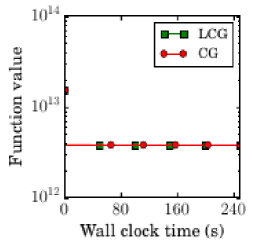
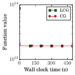
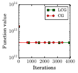
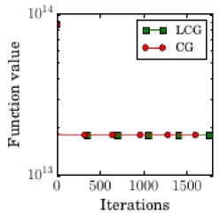
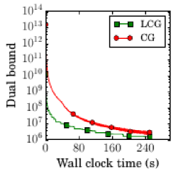
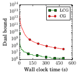
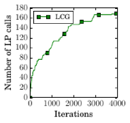
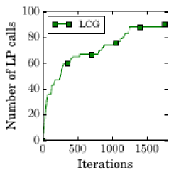
cache hit rate: $95.72\%$	cache hit rate: $94.83\%$

Figure 1: LCG vs. CG on small netgen instances netgen 08a (left) and netgen 10a (right) with quadratic objective functions. In both cases both algorithms are able to reduce the function value very fast, however the dual bound or Wolfe gap is reduced much faster by LCG. Observe that the vertical axis is given with a logscale.

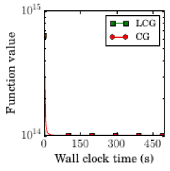
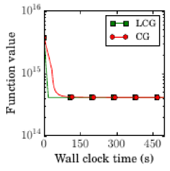
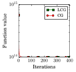
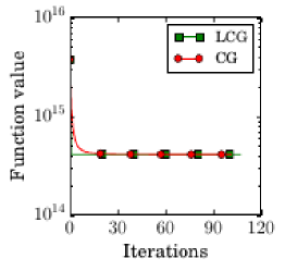
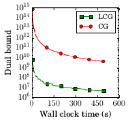
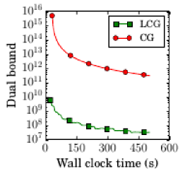
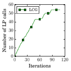
cache hit rate: $86.43\%$	cache hit rate: $50.00\%$

Figure 2: LCG vs. CG on medium sized netgen instances netgen 12b (left) and netgen 14a (right) with quadratic objective functions. The behavior of both versions on these instances is very similar to the small netgen instances (Figure 1), however both in the function value and the dual bound the difference between the lazy and the non-lazy version is more prominent. Again, we used a logscale for the vertical axis.

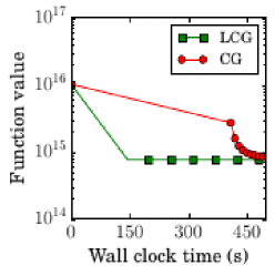
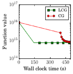
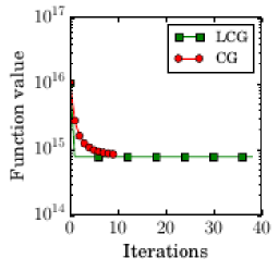
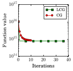
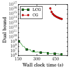
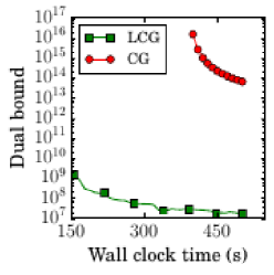
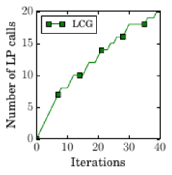
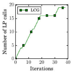
cache hit rate: $48.72\%$	cache hit rate: $50.00\%$

Figure 3: LCG vs. CG on large netgen instances netgen 16a (left) and netgen 16b (right) with quadratic objective functions. In both cases the difference in function value between the two versions of the algorithm is large. In the dual bound the performance of the lazy version is multiple orders of magnitude better than the performance of the non-lazy counterpart. The cache hit rates for these two instances are lower due to the high dimension of the polytope.

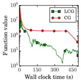
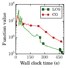
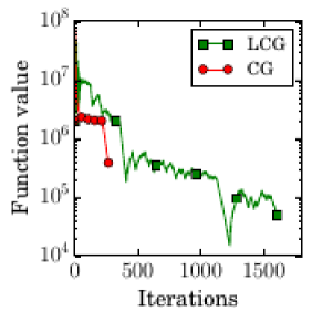
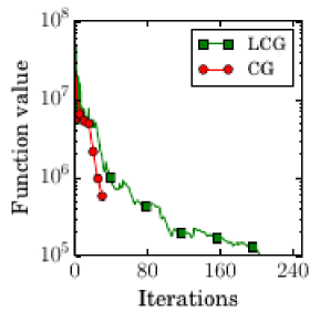
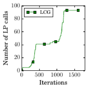
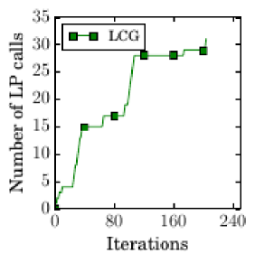
cache hit rate: $94.24\%$	cache hit rate: $84.80\%$

Figure 4: LCG vs. CG on two matrix completion instances. We solve the problem as given in Equation (25) with the paramters $n=3000$, $m=1000$, $r=10$ and $R=30000$ for the left instance and $n=10000$, $m=100$, $r=10$ and $R=10000$ for the right instance. In both cases the lazy version is slower in interations, however significantly faster in wall clock time.

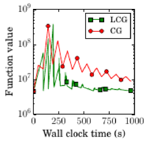
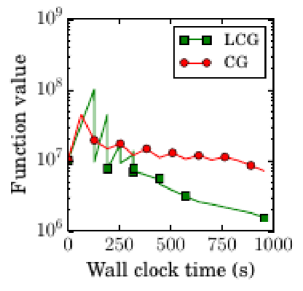
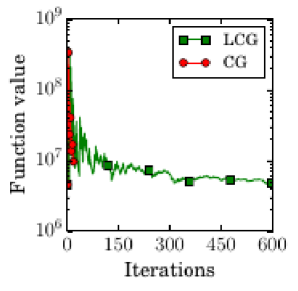
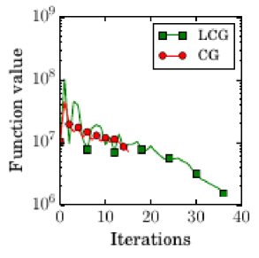
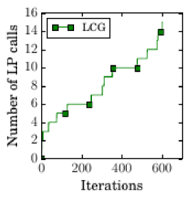
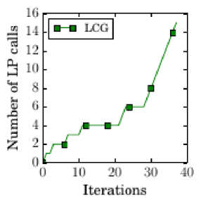
cache hit rate: $97.50\%$	cache hit rate: $59.46\%$

Figure 5: LCG vs. CG on two more matrix completion instances. The parameters for Equation (25) are given by $n=5000$, $m=4000$, $r=10$ and $R=50000$ for the left instance and $n=100$, $m=20000$, $r=10$ and $R=15000$ for the right instance. In both of these cases the performance of the lazy and the non-lazy version are comparable in interations, however in wall clock time the lazy version reaches lower function values faster.

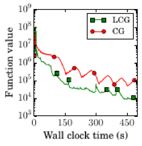
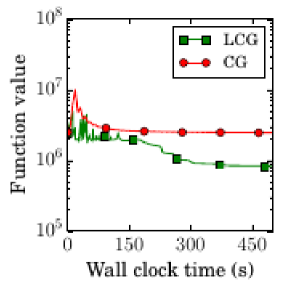
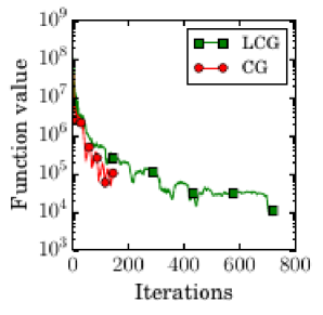
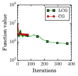
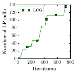
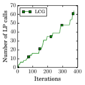
cache hit rate: $80.80\%$	cache hit rate: $82.98\%$

Figure 6: LCG vs. CG on our fifth and sixth instance of the matrix completion problem. The parameters are $n=5000$, $m=100$, $r=10$ and $R=15000$ for the left instance and $n=3000$, $m=2000$, $r=10$ and $R=10000$ for the right instance. The behavior is very similar to Figure 5. similar performance over iterations however advantages for the lazy version in wall clock time.

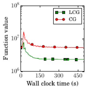
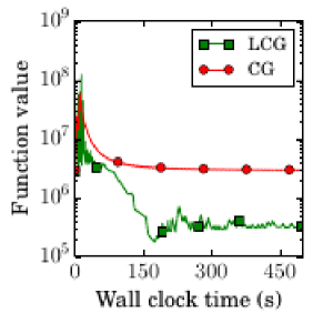
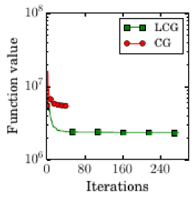
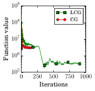
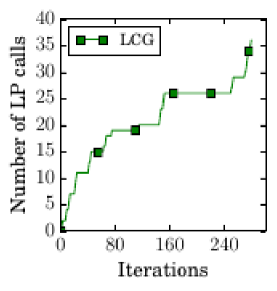
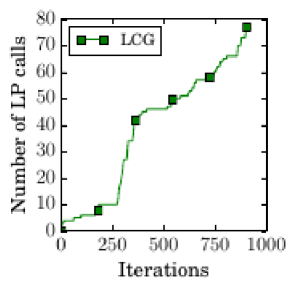
cache hit rate: $87.10\%$	cache hit rate: $91.55\%$

Figure 7: LCG vs. CG on the final two matrix completion instances. The parameters are $n=10000$, $m=1000$, $r=10$ and $R=1-000$ for the left instance and $n=5000$, $m=1000$, $r=10$ and $R=30000$ for the right instance. On the left in both measures, instances and wall clock time, the lazy version performs better than the non-lazy counterpart, due to a suboptimal direction at the beginning with a fairly large step size in the non-lazy version.

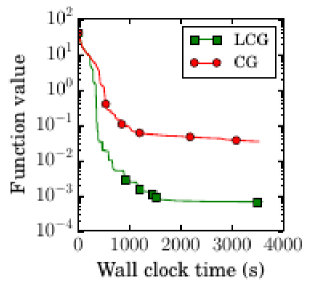
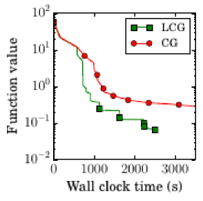
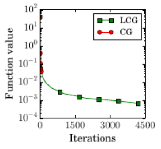
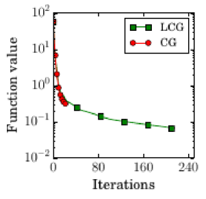
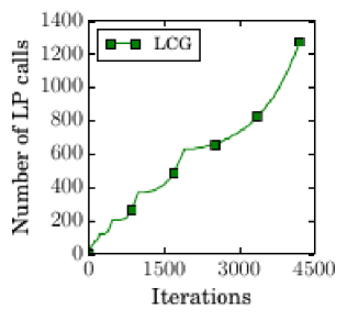
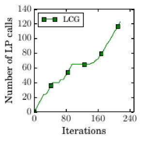
cache hit rate: $69.46\%$	cache hit rate: $43.06\%$

Figure 8: LCG vs. CG on structured regression problems with feasible regions being a TSP polytope over $11$ nodes (left) and $12$ nodes (right). In both cases LCG is significantly faster in wall-clock time.

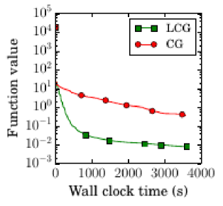
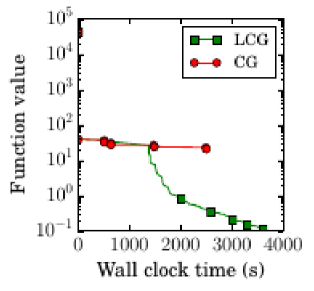
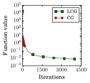
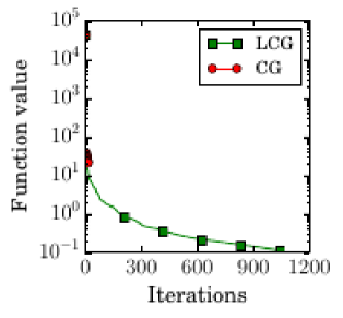
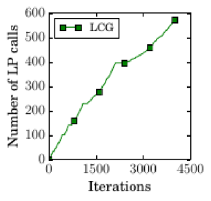
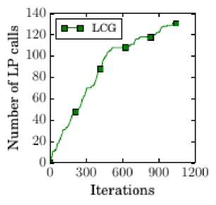
cache hit rate: $85.61\%$	cache hit rate: $87.48\%$

Figure 9: LCG vs. CG on structured regression instances using cut polytopes over a graph on $23$ nodes (left) and over $28$ nodes (right) as feasible region. In both instances LCG performs significantly better than CG.

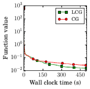
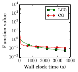
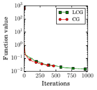
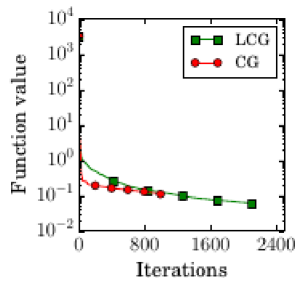
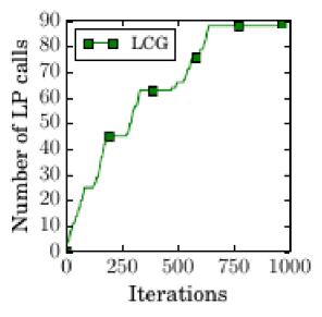
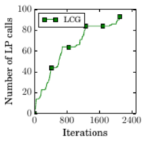
cache hit rate: $90.83\%$	cache hit rate: $95.59\%$

Figure 10: LCG vs. CG on structured regression instances with extended formulation of the spanning tree problem on a $10$ node graph on the left and a $15$ node graph on the right.

Pairwise Conditional Gradient Algorithm

As we inherit structural restrictions of PCG on the feasible region, the problem repertoire is limited in this case. We tested the Pairwise Conditional Gradient algorithm on the structured regression problem with feasible regions from the MIPLIB instances eil33-2, air04, eilB101, nw04, disctom, m100n500k4r1 (Figures 11, 12 and 13).

Again similarly to the vanilla Frank-Wolfe algorihtm, we observed a significant improvement in wall-clock time of LPCG compared to CG, due to the faster iteration of the lazy algorithm.

eil33-2, $4516$ dimensions	air04, $8904$ dimensions
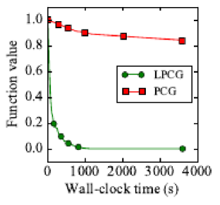
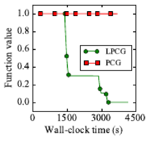
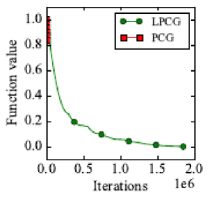
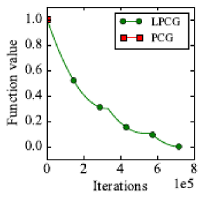
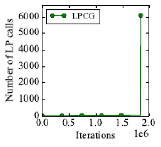
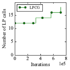
cache hit rate: $99.8\%$	cache hit rate: $99.999\%$

Figure 11: LPCG vs. PCG on two MIPLIB instances eil33-2 and air04. LPCG converges very fast, making millions of iterations with a relatively few oracle calls, while PCG completed only comparably few iterations due to the time-consuming oracle calls. This clearly illustrates the advantage of lazy methods when the cost of linear optimization is non-negligible. On the left, when reaching $\varepsilon$-optimality, LPCG performs many (negative) oracle calls to (re-)prove optimality; at that point one might opt for stopping the algorithm. On the right LPCG needed a rather long time for the initial bound tigthening of $\Phi_{0}$, before converging significantly faster than PCG.

eilB101, $2818$ dimensions	nw04, $87482$ dimensions
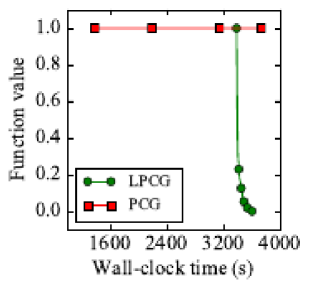
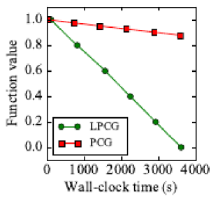
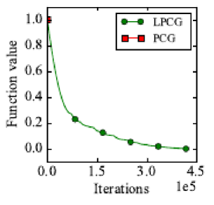
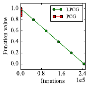
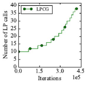
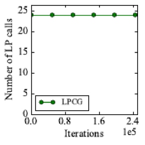
cache hit rate: $99.995\%$	cache hit rate: $99.995\%$

Figure 12: LPCG vs. PCG on MIPLIB instances eilB101 and nw04 with quadratic loss functions. For the eilB101 instance, LPCG spent most of the time tightening $\Phi_{0}$, after which it converged very fast, while PCG was unable to complete a single iteration even solving the problem only approximately. For the nw04 instance LPCG needed no more oracle calls after an initial phase, while significantly outperforming PCG.

disctom, $10000$ dimensions	m100n500k4r1, $600$ dimensions
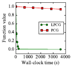
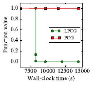
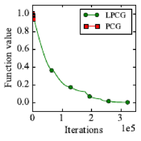
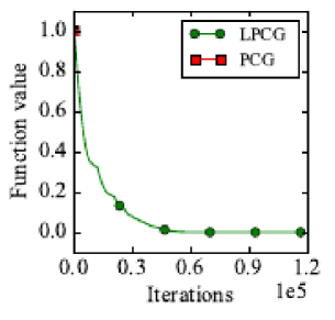
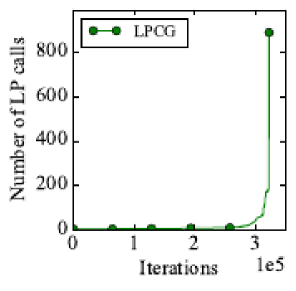
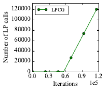
cache hit rate: $99.9\%$	cache hit rate: $48.4\%$

Figure 13: LPCG vs. PCG on MIPLIB instances disctom and m100n500k4r1. After very fast convergence, there is a huge increase in the number of oracle calls for the lazy algorithm LPCG due to reaching $\varepsilon$-optimality as explained before. On the right the initial bound tightening for $\Phi_{0}$ took a considerable amount of time but then convergence is almost instantaneous.

7.1.2 Online Results

Additionally to the quadratic objective functions above we tested the online version on random linear functions $cx+b$ with $c\in[-1,+1]^{n}$ and $b\in[0,1].$ For online algorithms, each experiment used a random sequence of $100$ different random loss functions. In every figure the left column uses linear loss functions, while the right one uses quadratic loss functions over the same polytope. As customary, we did not use line search here but used the respective prescribed step sizes.

As an instance of the structured regression problem we used the flow-based formulation for Hamiltonian cycles in graphs, i.e., the traveling salesman problem (TSP) for graphs with $11$ and $16$ nodes (Figures 14 and 15).

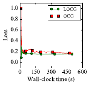
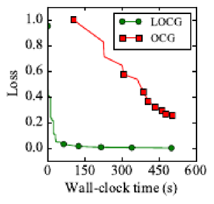
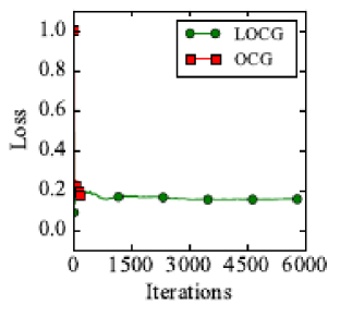
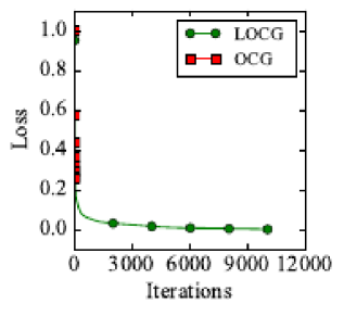
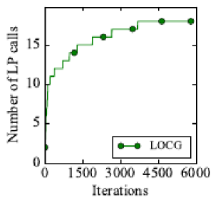
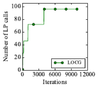
cache hit rate: $99.7\%$	cache hit rate: $99.0\%$

Figure 14: LOCG vs. OCG over TSP polytope for a graph with $11$ nodes as feasible region and with a $500$ seconds time limit. OCG completed only a few iterations, resulting in a several times larger final loss for quadratic loss functions (right). Notice that with time LOCG needed fewer and fewer LP calls.

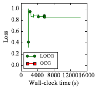
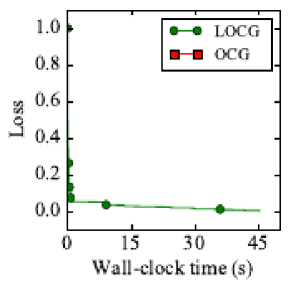
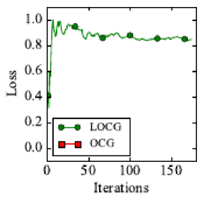
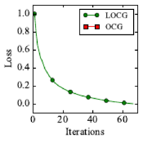
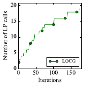
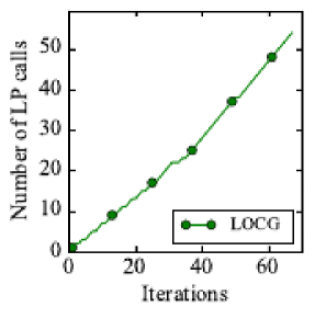
cache hit rate: $89.1\%$	cache hit rate: $20.6\%$

Figure 15: LOCG vs. OCG over TSP polytope for a graph with $16$ nodes with a time limit of $7200$ seconds. OCG was not able to complete a single iteration and in the quadratic case (right) even LOCG could not complete any more iteration after 50s. The quadratic losses nicely demonstrate speed improvements (mostly) through early termination of the linear optimization as the cache rate is only $20.6\%$.

For these small instances, the oracle problem can be solved in reasonable time. Another instance of the structured regression problem uses the standard formulation of the cut polytope for graphs with $23$ and $28$ nodes as the feasible region (Figures 16 and 17).

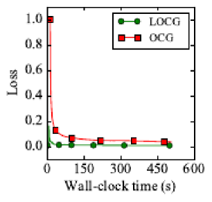
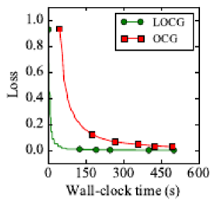
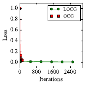
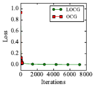
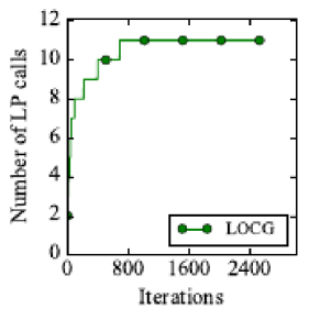
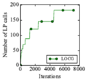
cache hit rate: $99.6\%$	cache hit rate: $97.5\%$

Figure 16: LOCG vs. OCG on the cut polytope for a graph with 23 nodes. Both LOCG and OCG converge to the optimum in a few iterations for linear losses, while LOCG is remarkably faster for quadratic losses. As can be seen here the advantage of lazy algorithms strongly correlates with the difficulty of linear optimization. For linear losses, remarkably LOCG needed no LP oracle calls after one third of the time.

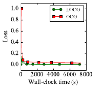
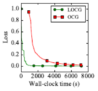
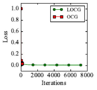
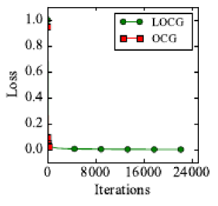
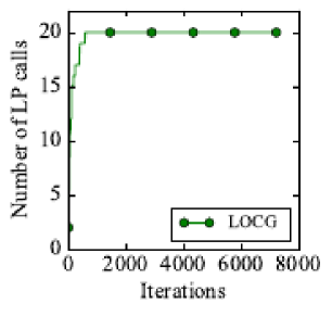
cache hit rate: $99.7\%$	cache hit rate: $98.6\%$

Figure 17: LOCG vs. OCG over cut polytope for a 28-node graph. As for the smaller problem, this also illustrates the advantage of lazy algorithms when linear optimization is expensive. Again, LOCG needed no oracle calls after a small initial amount of time.

We also tested our algorithm on are the quadratic unconstrained boolean optimization (QUBO) instances defined on Chimera graphs (Dash, 2013), which are available at http://researcher.watson.ibm.com/researcher/files/us-sanjeebd/chimera-data.zip. The instances are relatively hard albeit their rather small size and in general the problem is NP-hard. (Figure 18 and 19).

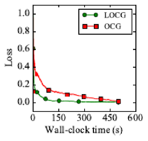
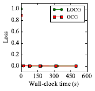
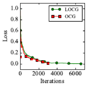
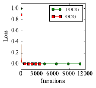
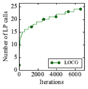
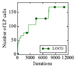
cache hit rate: $99.6\%$	cache hit rate: $98.5\%$

Figure 18: LOCG vs. OCG on a small QUBO instance. For quadratic losses (right), both algorithms converged very fast while LOCG still has a significant edge. This time, for linear losses (left) LOCG is noticeably faster than OCG.

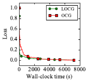
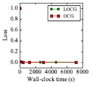
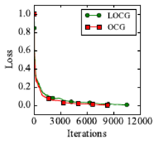
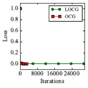
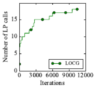
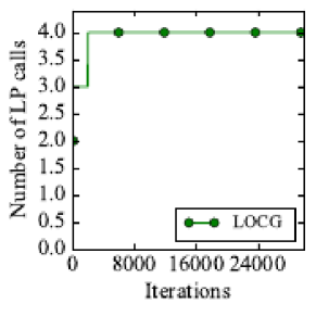
cache hit rate: $99.8\%$	cache hit rate: $99.99\%$

Figure 19: LOCG vs. OCG on a large QUBO instance. Both algorithms converge fast to the optimum. Interestingly, LOCG only performs $4$ LP calls.

One instance of the video colocalization problem uses a path polytope from http://lime.cs.elte.hu/~kpeter/data/mcf/netgen/ that was generated with the netgen graph generator (Figure 20). Most of these instances are very large-scale minimum cost flow instances with several tens of thousands nodes in the underlying graphs, therefore solving still takes considerable time despite the problem being in P.

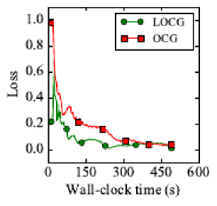
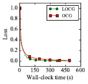
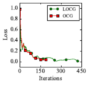
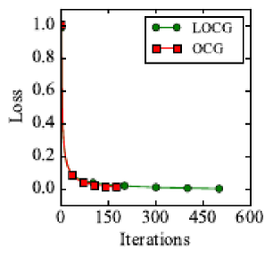
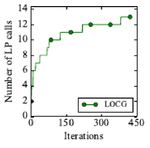
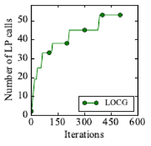
cache hit rate: $97.0\%$	cache hit rate: $89.6\%$

Figure 20: LOCG vs. OCG over a path polytope. Similar convergence rate in the number of iterations, but significant difference in terms of wall-clock time.

We tested on the structured regression problems with the MIPLIB (Achterberg et al., 2006; Koch et al., 2011)) instances eil33-2 (Figure 21) and air04 (Figure 22) as feasible regions.

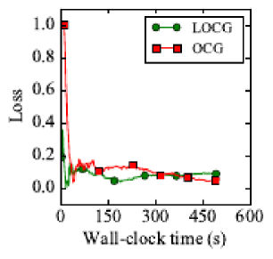
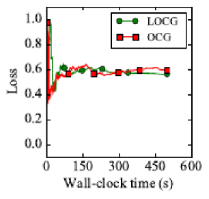
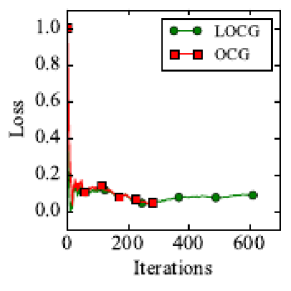
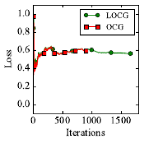
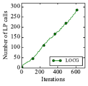
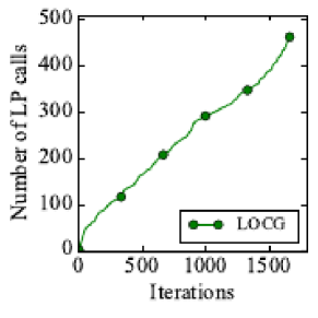
cache hit rate: $53.1\%$	cache hit rate: $72.2\%$

Figure 21: LOCG vs. OCG on the MIPLIB instance eil33-2. All algorithms performed comparably, due to fast convergence in this case.

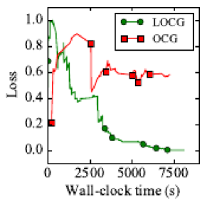
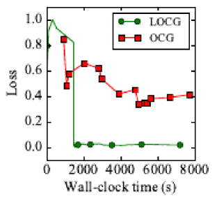
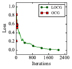
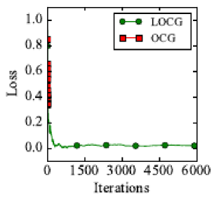
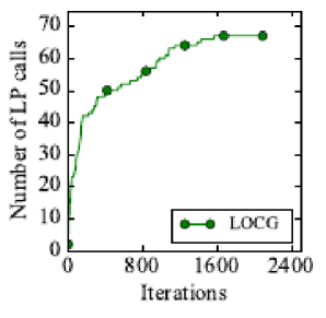
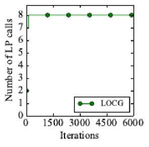
cache hit rate: $96.8\%$	cache hit rate: $99.9\%$

Figure 22: LOCG vs. OCG on the MIPLIB instance air04. LOCG clearly outperforms OCG as the provided time was not enough for OCG to complete the necessary number of iterations for entering reasonable convergence.

Finally, for the spanning tree problem, we used the well-known extended formulation with $O(n^{3})$ inequalities for an $n$-node graph. We considered graphs with 10 and 25 nodes (Figures 23 and 24).

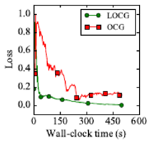
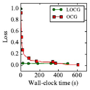
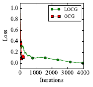
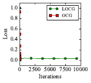
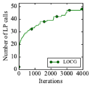
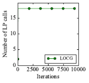
cache hit rate: $98.8\%$	cache hit rate: $99.8\%$

Figure 23: LOCG vs. OCG on a spanning tree instance for a 10-node graph. LOCG makes significantly more iterations, few oracle calls, and converges faster in wall-clock time.

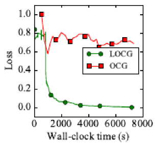
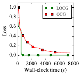
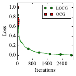
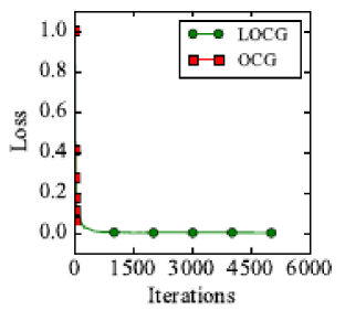
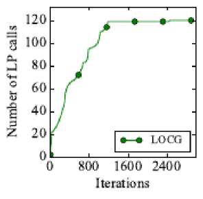
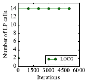
cache hit rate: $95.9\%$	cache hit rate: $99.7\%$

Figure 24: LOCG vs. OCG over a spanning tree instance for a 25-node graph. On the left, early fluctuation can be observed, bearing no consequence for later convergence rate. OCG did not get past this early stage. In both cases LOCG converges significantly faster.

We observed that similarly to the offline case while OCG and LOCG converge comparably in the number of iterations, the lazy LOCG performed significantly more iterations; for hard problems, where linear optimization is costly and convergence requires a large number of iterations, this led LOCG converging much faster in wall-clock time. In extreme cases OCG could not complete even a single iteration. This is due to LOCG only requiring some good enough solution, whereas OCG requires a stronger guarantee. This is reflected in faster oracle calls for LOCG.

7.2 Performance improvements, parameter sensitivity, and tuning

7.2.1 Effect of caching

As mentioned before, lazy algorithms have two improvements: caching and early termination. Here we depict the effect of caching in Figure 25, comparing OCG (no caching, no early termination), LOCG (caching and early termination) and LOCG (only early termination) (see Algorithm 8). We did not include a caching-only OCG variant, because caching without early termination does not make much sense: in each iteration a new linear optimization problem has to be solved; previous solutions can hardly be reused as they are unlikely to be optimal for the new linear optimization problem.

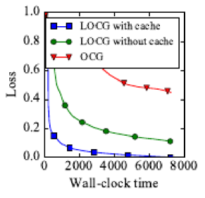
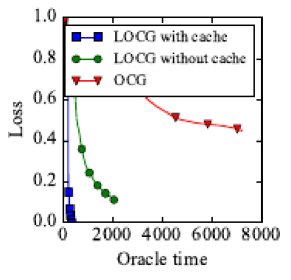
Figure 25: Performance gain due to caching and early termination for online optimization over a maximum cut problem with linear losses. The red line is the OCG baseline, the green one is the lazy variant using only early termination, and the blue one uses caching and early termination. Left: loss vs. wall-clock time. Right: loss vs. total time spent in oracle calls. Time limit was $7200$ seconds. Caching allows for a significant improvement in loss reduction in wall-clock time. The effect is even more obvious in oracle time as caching cuts out a large number of oracle calls.

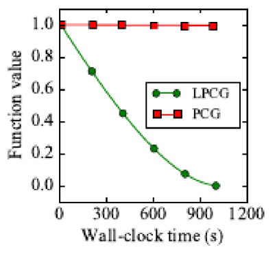
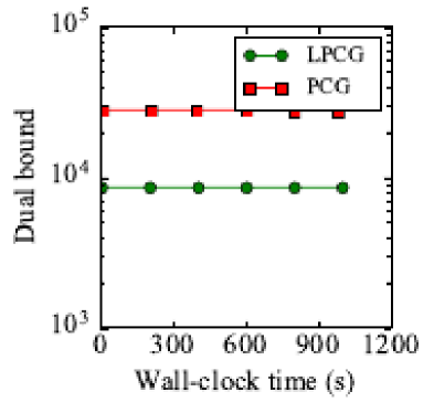
Figure 27: Performance on a large instance of the video colocalization problem using PCG and its lazy variant. We observe that lazy PCG is significantly better both in terms of function value and dual bound. Recall that the function value is normalized between $[0,1]$.

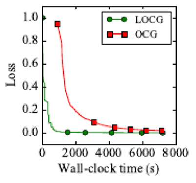
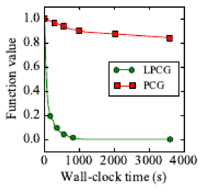
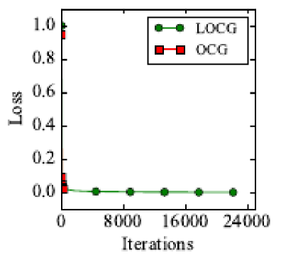
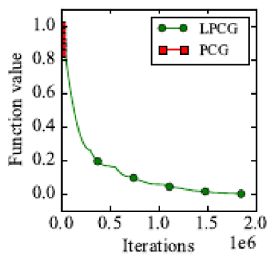
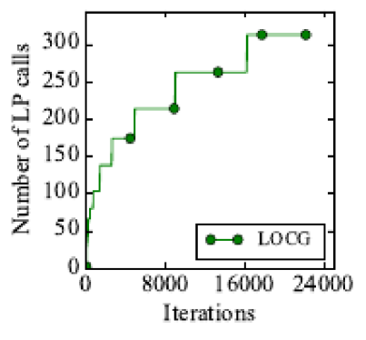
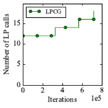
Figure 29: Performance of the two lazified variants LOCG (left column) and LPCG (right column). The feasible regions are a cut polytope on the left and the MIPLIB instance air04 on the right. The objective functions are in both cases quadratic, on the left randomly chosen in every step. We show the performance over wall clock time in seconds (first row) and over iterations (second row). The last row shows the number of call to the linear optimization oracle. The lazified versions perform significantly better in wall clock time compared to the non-lazy counterparts.

7.2.2 Effect of $K$

If the parameter $K$ of the oracle can be chosen, which depends on the actual oracle implementation, then we can increase $K$ to bias the algorithm towards performing more positive calls. At the same time the steps get shorter. As such there is a natural trade-off between the cost of many positive calls vs. a negative call. We depict the impact of the parameter choice for $K$ in Figure 30.

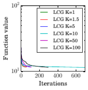
Figure 30: Impact of the oracle approximation parameter $K$ depicted for the Lazy CG algorithm. We can see that increasing $K$ leads to a deterioration of progress in iterations but improves performance in wall-clock time. The behavior is similar for other algorithms.

7.2.3 Paramter-free vs. textbook variant

For illustrative purposes, we compare the textbook variant of the lazy conditional gradient (Algorithm 3) with its parameter-free counterpart (Algorithm 7) in Figure 31. The parameter-free variant outperforms the textbook variant due to the active management of $\Phi$ combined with line search.

Similar parameter-free variants can be derived for the other algorithms; see discussion in Section 4.

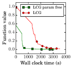
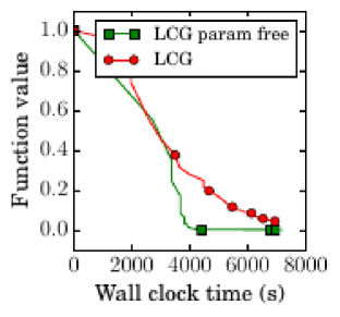
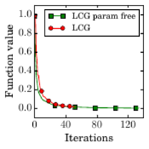
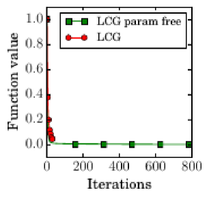
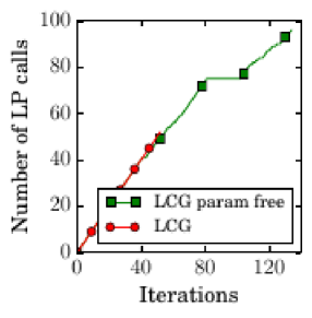
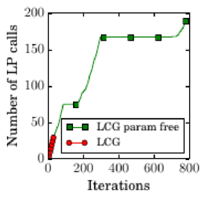
Figure 31: Comparison of the ‘textbook’ variant of the Lazy CG algorithm (Algorithm 3) vs. the Parameter-free Lazy CG (Algorithm 7) depicted for two sample instances to demonstrate behavior. The parameter-free variant usually has a slighlty improved behavior in terms of iterations and a significantly improved behavior in terms of wall-clock performance. In particular, the parameter-free variant can execute significantly more oracle calls, due to the $\Phi$-halving strategy and the associated bounded number of negative calls (see Theorem 4.3).

8 Final Remarks

If a given baseline algorithm works over general compact convex sets $P$, then so does the lazified version. In fact, as the lazified algorithm runs, it produces a polyhedral approximation of the set $P$ with very few vertices (subject to optimality vs. sparsity tradeoffs; see (Jaggi, 2013, Appendix C)).

Moreover, the weak separation oracle does not need to return extreme points. All algorithms also work with maximal solutions that are not necessarily extremal (e.g., lying in a higher-dimensional face). However, in that case we lose the desirable property that the final solution is a sparse convex combination of extreme points (typically vertices in the polyhedral setup).

We would also like to briefly address potential downsides of our approach. In fact, we believe the right perspective is the following: when using the lazy oracle over the LP oracle, we obtain potentially weaker approximations $v_{t}-x_{t}$ of the true gradient $\nabla f(x_{t})$ compared to solving the actual LP, but the computation might be much faster. This is the tradeoff that one has to consider: working with weaker approximations (which implies potentially less progress per iteration) vs. potentially significantly faster computation of the approximations. If solving the LP is expensive than lazification will be usually very beneficial, if the LP is very cheap as in the case of $P=[0,1]^{n}$ or $P=\Delta_{n}$ being the probability simplex, then lazification might be slower.

A related remark in this context is that once the lazified algorithm has obtained vertices $x_{1},\dots,x_{m}$ of $P$, so that the minimizer $x^{*}$ of $f$ satisfies $x^{*}\in\text{conv}\{x_{1},\dots,x_{m}\}$, then from that point onwards no actual calls to the true LP oracle have to be performed anymore for primal progress and the algorithm will only use cache calls; the only remaining true LP calls are at most a logarithmic number for dual progress updates of the $\Phi_{t}$.

References

• Achterberg et al. [2006] T. Achterberg, T. Koch, and A. Martin. MIPLIB 2003. Operations Research Letters, 34(4):361–372, 2006. doi: 10.1016/j.orl.2005.07.009. URL http://www.zib.de/Publications/abstracts/ZR-05-28/.
• Audibert et al. [2013] J.-Y. Audibert, S. Bubeck, and G. Lugosi. Regret in online combinatorial optimization. Mathematics of Operations Research, 39(1):31–45, 2013.
• Bodic et al. [2015] P. L. Bodic, J. W. Pavelka, M. E. Pfetsch, and S. Pokutta. Solving MIPs via scaling-based augmentation. arXiv preprint arXiv:1509.03206, 2015.
• Braun et al. [2017] G. Braun, S. Pokutta, and D. Zink. Lazifying Conditional Gradient Algorithms. Proceedings of ICML, 2017.
• Cohen and Hazan [2015] A. Cohen and T. Hazan. Following the perturbed leader for online structured learning. In Proceedings of the 32nd International Conference on Machine Learning (ICML-15), pages 1034–1042, 2015.
• Dash [2013] S. Dash. A note on QUBO instances defined on Chimera graphs. preprint arXiv:1306.1202, 2013.
• Frank and Tardos [1987] A. Frank and É. Tardos. An application of simultaneous Diophantine approximation in combinatorial optimization. Combinatorica, 7(1):49–65, 1987.
• Frank and Wolfe [1956] M. Frank and P. Wolfe. An algorithm for quadratic programming. Naval research logistics quarterly, 3(1-2):95–110, 1956.
• Freund and Grigas [2016] R. M. Freund and P. Grigas. New analysis and results for the Frank–Wolfe method. Mathematical Programming, 155(1):199–230, 2016. ISSN 1436-4646. doi: 10.1007/s10107-014-0841-6. URL http://dx.doi.org/10.1007/s10107-014-0841-6.
• Garber and Hazan [2013] D. Garber and E. Hazan. A linearly convergent conditional gradient algorithm with applications to online and stochastic optimization. arXiv preprint arXiv:1301.4666, 2013.
• Garber and Meshi [2016] D. Garber and O. Meshi. Linear-memory and decomposition-invariant linearly convergent conditional gradient algorithm for structured polytopes. arXiv preprint, arXiv:1605.06492v1, May 2016.
• Grötschel and Lovász [1993] M. Grötschel and L. Lovász. Combinatorial optimization: A survey, 1993.
• Gupta et al. [2016] S. Gupta, M. Goemans, and P. Jaillet. Solving combinatorial games using products, projections and lexicographically optimal bases. arXiv preprint arXiv:1603.00522, 2016.
• Gurobi Optimization [2016] Gurobi Optimization. Gurobi optimizer reference manual version 6.5, 2016. URL https://www.gurobi.com/documentation/6.5/refman/.
• Hazan [2016] E. Hazan. Introduction to online convex optimization. Foundations and Trends in Optimization, 2(3–4):157–325, 2016. doi: 10.1561/2400000013. URL http://ocobook.cs.princeton.edu/.
• Hazan and Kale [2012] E. Hazan and S. Kale. Projection-free online learning. arXiv preprint arXiv:1206.4657, 2012.
• Jaggi [2013] M. Jaggi. Revisiting Frank–Wolfe: Projection-free sparse convex optimization. In Proceedings of the 30th International Conference on Machine Learning (ICML-13), pages 427–435, 2013.
• Joachims et al. [2009] T. Joachims, T. Finley, and C.-N. J. Yu. Cutting-plane training of structural SVMs. Machine Learning, 77(1):27–59, 2009.
• Joulin et al. [2014] A. Joulin, K. Tang, and L. Fei-Fei. Efficient image and video co-localization with Frank-Wolfe algorithm. In European Conference on Computer Vision, pages 253–268. Springer, 2014.
• Kalai and Vempala [2005] A. Kalai and S. Vempala. Efficient algorithms for online decision problems. Journal of Computer and System Sciences, 71(3):291–307, 2005.
• Koch et al. [2011] T. Koch, T. Achterberg, E. Andersen, O. Bastert, T. Berthold, R. E. Bixby, E. Danna, G. Gamrath, A. M. Gleixner, S. Heinz, A. Lodi, H. Mittelmann, T. Ralphs, D. Salvagnin, D. E. Steffy, and K. Wolter. MIPLIB 2010. Mathematical Programming Computation, 3(2):103–163, 2011. doi: 10.1007/s12532-011-0025-9. URL http://mpc.zib.de/index.php/MPC/article/view/56/28.
• Lacoste-Julien and Jaggi [2015] S. Lacoste-Julien and M. Jaggi. On the global linear convergence of Frank–Wolfe optimization variants. In C. Cortes, N. D. Lawrence, D. D. Lee, M. Sugiyama, and R. Garnett, editors, Advances in Neural Information Processing Systems, volume 28, pages 496–504. Curran Associates, Inc., 2015. URL http://papers.nips.cc/paper/5925-on-the-global-linear-convergence-of-frank-wolfe-optimization-variants.pdf.
• Lacoste-Julien et al. [2013] S. Lacoste-Julien, M. Jaggi, M. Schmidt, and P. Pletscher. Block-coordinate Frank–Wolfe optimization for structural SVMs. In ICML 2013 International Conference on Machine Learning, pages 53–61, 2013.
• Lan and Zhou [2014] G. Lan and Y. Zhou. Conditional gradient sliding for convex optimization. Optimization-Online preprint (4605), 2014.
• Levitin and Polyak [1966] E. S. Levitin and B. T. Polyak. Constrained minimization methods. USSR Computational mathematics and mathematical physics, 6(5):1–50, 1966.
• Neu and Bartók [2013] G. Neu and G. Bartók. An efficient algorithm for learning with semi-bandit feedback. In Algorithmic Learning Theory, pages 234–248. Springer, 2013.
• Oertel et al. [2014] T. Oertel, C. Wagner, and R. Weismantel. Integer convex minimization by mixed integer linear optimization. Oper. Res. Lett., 42(6-7):424–428, 2014.
• Osokin et al. [2016] A. Osokin, J.-B. Alayrac, I. Lukasewitz, P. K. Dokania, and S. Lacoste-Julien. Minding the gaps for block Frank–Wolfe optimization of structured SVMs. ICML 2016 International Conference on Machine Learning / arXiv preprint arXiv:1605.09346, 2016.
• Pokutta [2017] S. Pokutta. Smooth convex optimization via geometric scaling. preprint, 2017.
• Schulz and Weismantel [2002] A. S. Schulz and R. Weismantel. The complexity of generic primal algorithms for solving general integer programs. Mathematics of Operations Research, 27(4):681–692, 2002.
• Schulz et al. [1995] A. S. Schulz, R. Weismantel, and G. M. Ziegler. 0/1-integer programming: Optimization and augmentation are equivalent. In Algorithms – ESA ’95, Proceedings, pages 473–483, 1995.
• Shah et al. [2015] N. Shah, V. Kolmogorov, and C. H. Lampert. A multi-plane block-coordinate Frank–Wolfe algorithm for training structural SVMs with a costly max-oracle. In Proceedings of the IEEE Conference on Computer Vision and Pattern Recognition, pages 2737–2745, 2015.