We study the evolution of the hybrid entangled squeezed states of the qubit-oscillator system in the strong coupling domain. Following the adiabatic approximation we obtain the reduced density matrices of the qubit and the oscillator degrees of freedom. The oscillator reduced density matrix is utilized to calculate the quasiprobability distributions such as the Sudarshan-Glauber diagonal $P$-representation, the Wigner $W$-distribution, and the nonnegative Husimi $Q$-function. The negativity associated with the $W$-distribution acts as a measure of the nonclassicality of the state. The existence of the multiple time scales induced by the interaction introduces certain features in the bipartite system. In the strong coupling regime the transient evolution to low entropy configurations reveals brief emergence of nearly pure kitten states that may be regarded as superposition of uniformly separated distinguishable squeezed coherent states. However, the quantum fluctuations with a short time period engender bifurcation and subsequent rejoining of these peaks in the phase space. The abovementioned doubling of the number of peaks increases the entropy to its near maximal value. Nonetheless, these states characterized by high entropy values, are endowed with a large negativity of the $W$-distribution that points towards their non-Gaussian behavior. This may be ascertained by the significantly large Hilbert-Schmidt distance between the oscillator state and an ensemble of most general statistical mixture of squeezed Gaussian states possessing nearly identical second order quadrature moments as that of the oscillator.

Keyword: Hybrid entangled squeezed state, Multiple time scales, Hilbert-Schmidt distance, Reconstruction nearly pure kitten states, Non-Gaussian characteristics.

I Introduction

A two-level system (qubit) that interacts with a radiation field represented by a single oscillator mode is one of the important models in quantum optics. This model has been studied extensively under the rotating wave approximation [[1]] that holds good for the regime characterized by a weak coupling as well as a small detuning between the qubit and the oscillator frequencies. Recent experiments, however, probe the strong qubit-oscillator coupling domain, where the rotating wave approximation is not valid. Experimental realizations such as a nanoelectromechanical resonator capacitively coupled to a Cooper-pair box driven by microwave currents [[2], [3]], a quantum semiconductor microcavity displaying specific signatures of the ultrastrong coupling regime of the light-matter interaction [[4]], a flux-biased quantum circuit that utilizes the large inductance of a Josephson junction to produce an ultrastrong coupling with a coplanar waveguide resonator [[5]] fall in this group. Specifically, the superconducting qubits and circuits are adaptable for a wide range of parameters making them the preferred tools for building quantum simulators [[6]-[8]]. Additionally, the hybrid integrated circuits comprising of the atoms, spins, cavity photons, and the superconducting qubits with nanomechanical oscillators may facilitate fabrication of interfaces [[9]] in quantum communication network. The Hamiltonian of the strongly coupled qubit-oscillator system incorporates terms that do not preserve the excitation number. To analyze them in the regime where the high oscillator frequency dominates over the low (renormalized) qubit frequency, the authors of [[10, 11]] have advanced an adiabatic approximation scheme that utilizes the separation of the slow and fast degrees of freedom. This enables the decoupling of the full bipartite Hamiltonian into sectors related to each time scale, and admits approximate evaluation [[10]] of its eigenvalues and eigenstates.

The coupled qubit-oscillator system provides entanglement of the microscopic atomic state and the coherent states of the oscillator, say with opposite phases, that may be regarded as distinguishable and macroscopic for sufficiently high value of the coherent state amplitude [[12]]. These analogs of Schrödinger cat state are important in understanding the nature of the decoherence, the quantum-classical transition, and the quantum information processing with continuous variables. For instance, they enable non-destructive measurement [[13]] of the photon number in a field stored in a cavity. These states allow investigations [[14]] on the effects of decoherence by continuously varying the size of the prepared entangled states. Another important proposition is the quantum bus structure [[15]] where the hybrid entanglement is used as a tool to eliminate the direct qubit-qubit interactions while admitting a universally coupled continuous mode that mediates among qubits. Much experimental activity [[16]] is geared to observation of such hybrid entangled state. Realization of micro-macro entangled states via a controllable interaction of a single mode microwave cavity field with a superconducting qubit charge, and the subsequent appearance, caused by the measurement of the charge state of the qubit, of superposed macroscopically distinguished field modes have been proposed [[17]]. Recently, optical hybrid entanglement has been observed [[18]] by the superposition of non-Gaussian operations on distinct modes. The hybrid entanglement between two remote nodes residing in Hilbert spaces of different dimensionality has been realized [[19]] using a measurement based procedure. Controllable and deterministic generation of complex superposition of states are also investigated [[20]-[25]] using superconducting circuits.

On the other hand, the squeezed states of the harmonic oscillator involves the reduction of the fluctuation in one quadrature variable below the ground state uncertainty. This significant property has been used in quantum metrology towards improving the sensitivity of the interferometers [[26]]. Its role in the recent gravitational wave detection via high-power laser interferometers [[27]], and other possible future astronomical observations such as supernova explosions, makes it a key component for the future experiments. Squeezed states are also important in continuous variable quantum key distribution protocols [[28]], and it has been proven [[29]] that they can provide an enhancement compared to the coherent states. Moreover, they have recently been used as sensitive detectors for photon scattering recoil events at the single photon level [[30]]. Viewed in this context, the entangled squeezed wave packets in bipartite and multipartite systems hold much promise both for metrology and for continuous variable quantum information. Recently such states were experimentally realized [[31]] where the authors used the internal state-dependent forces to create a superposition of distinct squeezed oscillator wavepackets that are entangled with the electronic states of a single trapped ion.

The experimental scenario makes it imperative to study the evolution of the entangled squeezed wave packets in strongly coupled hybrid bipartite dynamical systems. The initial state is taken to be a superposition of distinct squeezed coherent states of the oscillator that are entangled with the qubit states. Towards understanding the dynamics of the quantum state, we utilize various quasi probability distributions on the phase space as preferred tools. For instance, the quasi probability $P$-distribution provides a diagonal representation [[32], [33]] of the oscillator reduced density matrix in a coherent state basis. The Wigner $W$-distribution [[34]] gives a connection between the classical and quantum dynamics as, unlike the classical (true) probability distributions, it may assume negative values. Its negativity [[35]] serves as an indicator of the nonclassicality of the quantum state. Moreover, investigations [[36]] on the nonclassical properties of the qudit cat states as revealed by their $W$-distributions in a $d$-dimensional truncated Fock space has been performed. In the phase space the nonnegativity of the suitably smoothed Husimi $Q$-function [[37]] facilitates the construction the semiclassical Wehrl entropy [[38]]. Also, it may be employed to provide a semiclassical measure of relative entropy between two suitable $Q$-functions. In the strong coupling regime where a quadratic approximation to the effective interaction holds, a long range quasi periodic time dependence in Wehrl entropy is manifest. This is much parallel to the behavior observed earlier [[39]-[42]] in the studies related to nonlinear self-interacting Kerr-like models. It is evident, say, from the Wigner $W$-distribution that at the rational submultiples of the long time period kitten-like configurations emerge in the phase space. However, multiple time scales present in our model introduces certain differences from earlier studies. Owing its origin to the interaction a short time quantum fluctuation is superposed on the long time quasi periodic behavior. This triggers a bifurcation and rejoining of the kitten states on the phase space. Quantum fluctuations in entropy in the short time period points towards recurrence of almost pure kitten states equi-rotated in the phase space, which are interspersed between near-maximal entropy states that register a doubling of the number of kittens. These high entropy states are, however, highly nonclassical as they are endowed with a large negativity of the $W$-distribution. Employing the Hilbert-Schmidt distance [[43]] between two quantum states we study this evolutionary aspect in detail.

The present manuscript is organized as follows: Starting with the hybrid entangled state of the qubit-oscillator bipartite system the reduced density matrix of the oscillator is considered under the adiabatic approximation in Sec. II. This density matrix yields the quasi probability distributions such as the Sudarshan-Glauber $P$-representation, the Wigner $W$-distribution, and the Husimi $Q$-function that admits a closed form evaluation in the weak coupling regime. The angular distribution in the phase space [[44], [45]] obtained via the matrix element of the oscillator density operator explicitly provides structure of the kitten states. For a later comparison between the quantum states the first two moments of the quadrature variables of the oscillator density matrix are obtained. The Sec. III is devoted to a detailed study of the kitten states emerging due to the presence of multiple time scales during the evolution in the strong coupling domain. We conclude in Sec. IV.

II The reduced density matrices and the phase space distributions

We study a coupled qubit-oscillator system with the Hamiltonian [[10], [11]] that reads in natural units $(\hbar=1)$ as follows:

$$H=-\frac{\Delta}{2}\sigma_{x}-\frac{\epsilon}{2}\sigma_{z}+\omega a^{\dagger}\,a+\lambda\sigma_{z}\,(a^{\dagger}+a),$$ (2.1)

where the harmonic oscillator with a frequency $\omega$ is described by the raising and lowering operators $(a^{\dagger},\,a|\hat{n}\equiv a^{\dagger}a)$. The spin variables $(\sigma_{x},\,\sigma_{z})$ characterize the qubit that is furnished with an energy splitting $\Delta$ and an external static bias $\epsilon$. Comparison of various types of the charge and the flux qubits depending on the relative strength of the energy parameters $\Delta$ and $\epsilon$ is given in [[6]]. The qubit-oscillator coupling strength is denoted by $\lambda$. The Fock states $\{\hat{n}|n\rangle=n|n\rangle,\,n=0,1,\ldots;\;a\,|n\rangle=\sqrt{n}\,|n-1\rangle,a^{\dagger}\,|n\rangle=\sqrt{n+1}\,|n+1\rangle\}$ provide the basis for the oscillator, whereas the pair of eigenstates $\sigma_{z}|\pm 1\rangle=\pm\,|\pm 1\rangle$ comprise the space of the qubit. To study the dynamical evolution of the system, we, in the present work, follow the adiabatic approximation [[10], [11]] that is based on the separation of the time scales governed by a high oscillator frequency and a comparatively low (renormalized) qubit splitting: $\omega\gg\Delta$.

Our choice of the initial state of the hybrid bipartite system admits the oscillator in squeezed coherent state while the entanglement and the interference phase relationship are activated by the parameter $\mathrm{c}\in\mathbb{C}$:

$$|\psi(0)\rangle=\dfrac{1}{\sqrt{1+|\mathrm{c}|^{2}}}\left(|1\rangle|\alpha,\xi\rangle+\mathrm{c}\,|-1\rangle|-\alpha,\xi\rangle\right),\quad|\alpha\rangle=\mathrm{D}(\alpha)|0\rangle,\,|\alpha,\xi\rangle=\mathrm{D}(\alpha)\mathrm{S}(\xi)|0\rangle,$$ (2.2)

where the displacement and the squeezing operators, respectively, read $\mathrm{D}(\alpha)=\exp(\alpha a^{\dagger}-\alpha^{*}a),\mathrm{S}(\xi)=\exp((\xi^{*}a^{2}-\xi a^{\dagger}{{}^{2}})/2),\,\alpha=\mathrm{Re}(\alpha)+i\,\mathrm{Im}(\alpha)\in\mathbb{C},\,\xi=r\exp(i\,\vartheta),\;r,\vartheta\in\mathbb{R}$.

The number states yield a mode expansion [[46]] of the squeezed coherent state:

$$|\alpha,\xi\rangle=\sum_{n=0}^{\infty}\mathcal{S}_{n}(\alpha,\xi)|n\rangle,\quad\mathcal{S}_{n}(\alpha,\xi)=\frac{1}{\sqrt{n!\;\mu}}\Big{(}\frac{\nu}{2\mu}\Big{)}^{\tfrac{n}{2}}\;\exp\Big{(}-\frac{1}{2}\,|\alpha|^{2}-\frac{\nu}{2\,\mu}\,\alpha^{*}{}^{2}\Big{)}\,\mathrm{H}_{n}\Big{(}\frac{\mu\alpha+\nu\alpha^{*}}{\sqrt{2\,\mu\,\nu}}\Big{)},$$ (2.3)

where the squeezing parameters read: $\mu=\cosh r,\nu=\exp(i\vartheta)\,\sinh r$, and the Hermite polynomials are given by the generating function: $\exp(2\,\mathsf{z}\mathsf{t}-\mathsf{t}^{2})=\sum_{n=0}^{\infty}\tfrac{\mathrm{H}_{n}(\mathsf{z})\,\mathsf{t}^{n}}{n!}$.

Employing the adiabatic approximation [[10]] the evolution of the initial state (2.2) may be constructed as:

$$|\psi(t)\rangle = \dfrac{1}{\sqrt{1+|\mathrm{c}|^{2}}}\exp\Big{(}-i\frac{\lambda}{\omega}\Big{(}\mathrm{Im}(\alpha)-\lambda t\Big{)}\Big{)}\sum_{n=0}^{\infty}\;\exp(-in\omega t)\;\mathcal{S}_{n}(\alpha_{+},\xi)\times$$ (2.4)

$$\times \Big{(}\mathsf{C}_{n}(t)\,|1,n_{+}\rangle+(-1)^{n}\,\mathsf{D}_{n}(t)\,|-1,n_{-}\rangle\Big{)},$$

where the displaced number states $|n_{\pm}\rangle=\mathrm{D}^{\dagger}\left(\pm\frac{\lambda}{\omega}\right)|n\rangle$ provide the decomposition basis. In the derivation of (2.4) the reflection property $\mathcal{S}_{n}(-\,\alpha,\xi)=(-1)^{n}\,\mathcal{S}_{n}(\alpha,\xi)$ has been used. The states $|n_{\pm}\rangle$ possess the overlap structure

$$\langle m_{-}|n_{+}\rangle=\begin{cases}(-1)^{m-n}\;\exp\left(-\frac{x}{2}\right)x^{\frac{m-n}{2}}\sqrt{n!/m!}\,\,L_{n}^{m-n}\left(x\right)&\forall\,m\geq n,\\ \exp\left(-\frac{x}{2}\right)x^{\frac{n-m}{2}}\sqrt{m!/n!}\,\,L_{m}^{n-m}\left(x\right)&\forall\,m<n,\end{cases}$$ (2.5)

where the associated Laguerre polynomials read: $L_{n}^{j}(x)=\sum_{k=0}^{n}\,(-1)^{k}\,\binom{n+j}{n-k}\,\frac{x^{k}}{k!}$. The time-dependent expansion coefficients in (2.4) are given by

$$\mathsf{C}_{n}(t)=\cos\chi_{n}t+\;i\;\dfrac{\tilde{\epsilon}-(-1)^{n}\,\mathrm{c}\,\delta_{n}}{\chi_{n}}\;\sin\chi_{n}t,\quad\mathsf{D}_{n}(t)=\mathrm{c}\,\cos\chi_{n}t-\;i\;\dfrac{\mathrm{c}\;\tilde{\epsilon}+(-1)^{n}\delta_{n}}{\chi_{n}}\;\sin\chi_{n}t,$$ (2.6)

where $\chi_{n}=\sqrt{\delta_{n}^{2}+\tilde{\epsilon}^{2}},\,\delta_{n}=-\tfrac{\widetilde{\Delta}}{2}L_{n}(x),\,L_{n}(x)\equiv L_{n}^{0}(x),\,x=\left(2\lambda/\omega\right)^{2},\,\widetilde{\Delta}=\Delta\exp\left(-x/2\right),\,\tilde{\epsilon}=\epsilon/2,\,\alpha_{+}=\alpha+\lambda/\omega$. The state (2.4) now directly imparts the bipartite density matrix: $\rho(t)=|\psi(t)\rangle\langle\psi(t)|$. Its partial trace over the qubit (oscillator) degree of freedom produces the reduced density matrices of the oscillator (qubit):

$$\rho_{\mathcal{O}}(t)\equiv\hbox{Tr}_{\mathcal{Q}}\,\rho(t),\quad\varrho_{\mathcal{Q}}(t)\equiv\hbox{Tr}_{\mathcal{O}}\,\rho(t).$$ (2.7)

The explicit construction of the oscillator reduced density matrix for the state (2.4) reads

$$\rho_{\mathcal{O}}(t) = \dfrac{1}{1+|\mathrm{c}|^{2}}\sum_{n,m=0}^{\infty}\mathcal{S}_{n}(\alpha_{+},\xi)\,\mathcal{S}_{m}(\alpha_{+},\xi)^{*}\Big{(}\mathsf{C}_{n}(t)\mathsf{C}_{m}(t)^{*}|n_{+}\rangle\langle m_{+}|$$ (2.8)

$$+(-1)^{n+m}\mathsf{D}_{n}(t)\mathsf{D}_{m}(t)^{*}|n_{-}\rangle\langle m_{-}|\Big{)}\exp\big{(}-i(n-m)\omega t\big{)}.$$

The time evolution of the qubit density matrix assumes the form

$$\rho_{\mathcal{Q}}(t)=\begin{pmatrix}\varrho_{1,1}&\zeta\\ \zeta^{*}&\varrho_{-1,-1}\end{pmatrix},$$ (2.9)

where the matrix elements are structured as

$$\varrho_{1,1} = \frac{1}{1+|\mathrm{c}|^{2}}\sum_{n=0}^{\infty}|\mathcal{S}_{n}(\alpha_{+},\xi)|^{2}\,|\mathsf{C}_{n}(t)|^{2},\quad\varrho_{-1,-1}=\frac{1}{1+|\mathrm{c}|^{2}}\sum_{n=0}^{\infty}|\mathcal{S}_{n}(\alpha_{+},\xi)|^{2}\,|\mathsf{D}_{n}(t)|^{2},$$

$$\zeta = \frac{1}{1+|\mathrm{c}|^{2}}\sum_{n,m=0}^{\infty}\!\!(-1)^{m}\mathcal{S}_{n}(\alpha_{+},\xi)\mathcal{S}_{m}(\alpha_{+},\xi)^{*}\mathsf{C}_{n}(t)\mathsf{D}_{m}(t)^{*}\langle m_{-}|n_{+}\rangle\,\exp(-i(n-m)\omega t).$$ (2.10)

The reduced density matrices (2.8, 2.9) satisfy the trace condition: $\mathrm{Tr}\varrho_{\mathcal{O}}(t)=1,\mathrm{Tr}\varrho_{\mathcal{Q}}(t)=1$. The oscillator reduced density matrix (2.8) facilitate the construction of the quasiprobability distributions. The pair of eigenvalues of the qubit density matrix (2.9) read: $\frac{1}{2}\pm\mathfrak{p},\;\mathfrak{p}=\sqrt{\tfrac{1}{4}-|\rho_{\mathcal{Q}}|}$, where its determinant is given by $|\rho_{\mathcal{Q}}|=\varrho_{1,1}\varrho_{-1,-1}-|\zeta|^{2}$. The eigenvalues allow us to compute its von Neumann entropy $S(\rho_{\cal Q})\equiv-\hbox{Tr}(\rho_{\cal Q}\,\log\rho_{\cal Q})$ as

$$S_{\cal Q}=-\left(\frac{1}{2}+\mathfrak{p}\right)\log\left(\frac{1}{2}+\mathfrak{p}\right)-\left(\frac{1}{2}-\mathfrak{p}\right)\log\left(\frac{1}{2}-\mathfrak{p}\right),$$ (2.11)

which measures the entanglement and the mixedness of the bipartite system. It is well-known [[47]] that if a composite system, comprising of two subsystems, resides in a pure state, the entropies of both subsystems are equal. In the present example this yields: $S_{\cal Q}=S_{\cal O}\equiv S$.

Another quantity that plays a key role in the analysis of the quantum states is Hilbert-Schmidt distance between any two arbitrary quantum density matrices $\rho_{1}$ and $\rho_{2}$ [[43]]:

$$d_{\mathrm{HS}}(\rho_{1},\rho_{2})=\left(\mathrm{Tr}(\rho_{1}^{2})+\mathrm{Tr}(\rho_{2}^{2})-2\;\mathrm{Tr}(\rho_{1}\rho_{2})\right)^{1/2}.$$ (2.12)

The above definition allows us to evaluate the distance between the oscillator states (2.8), say, at times $t_{1}$ and $t_{2}$ via the following norm and the superposition of states:

$$\mathrm{Tr}(\rho_{\mathcal{O}}(t)^{2}) = \frac{1}{(1+|\mathrm{c}|^{2})^{2}}\sum_{n,m=0}^{\infty}|\mathcal{S}_{n}(\alpha_{+},\xi)|^{2}|\mathcal{S}_{m}(\alpha_{+},\xi)|^{2}\quad\quad\times$$

$$\times\Big{(}|\mathsf{C}_{n}(t)|^{2}|\mathsf{C}_{m}(t)|^{2}+|\mathsf{D}_{n}(t)|^{2}|\mathsf{D}_{m}(t)|^{2}\Big{)}+2|\zeta(t)|^{2},$$

$$\mathrm{Tr}(\rho_{\mathcal{O}}(t_{1})\,\rho_{\mathcal{O}}(t_{2})) = \frac{1}{(1+|\mathrm{c}|^{2})^{2}}\Big{(}\sum_{n,m=0}^{\infty}|\mathcal{S}_{n}(\alpha_{+},\xi)|^{2}|\mathcal{S}_{m}(\alpha_{+},\xi)|^{2}\exp(-i\omega(n-m)(t_{1}-t_{2}))\times$$ (2.13)

$$\times\Big{(}\mathsf{C}_{n}(t_{1})\mathsf{C}_{m}(t_{1})^{*}\mathsf{C}_{m}(t_{2})\mathsf{C}_{n}(t_{2})^{*}+\mathsf{D}_{n}(t_{1})\mathsf{D}_{m}(t_{1})^{*}\mathsf{D}_{m}(t_{2})\mathsf{D}_{n}(t_{2})^{*}\Big{)}\Big{)}$$

$$+|\zeta(t_{1},t_{2})|^{2}+|\zeta(t_{2},t_{1})|^{2},$$

where

$$\zeta(t_{1},t_{2})=\frac{1}{1+|\mathrm{c}|^{2}}\!\sum_{n,m=0}^{\infty}\!\!(-1)^{m}\mathcal{S}_{n}(\alpha_{+},\xi)\mathcal{S}_{m}(\alpha_{+},\xi)^{*}\mathsf{C}_{n}(t_{1})\mathsf{D}_{m}(t_{2})^{*}\langle m_{-}|n_{+}\rangle\exp(-i\omega(nt_{1}-mt_{2})).$$ (2.14)

A. The Sudarshan-Glauber diagonal $P$-representation

Based on the overcompleteness of the coherent states the Sudarshan-Glauber $P$-representation [[32, 33]] is well-known to admit a diagonal construction of the oscillator density matrix in the coherent state basis:

$$\rho_{\mathcal{O}}=\int P(\beta,\beta^{*})\,|\beta\rangle\langle\beta|\,\mathrm{d}^{2}\beta,$$ (2.15)

where the normalizability condition reads $\int P(\beta,\beta^{*})\,\mathrm{d}^{2}\beta=1$. For an arbitrary quantum state the relation (2.15) may be inverted and the diagonal $P$-representation is uniquely expressed [[48]] as the following distribution:

$$P(\beta,\beta^{*})=\dfrac{\exp(|\beta|^{2})}{\pi^{2}}\int\langle-\gamma|\rho_{\mathcal{O}}|\gamma\rangle\,\exp(|\gamma|^{2})\,\exp(\beta\gamma^{*}-\beta^{*}\gamma)\,\mathrm{d}^{2}\gamma.$$ (2.16)

For the reduced oscillator density matrix (2.8) the Fourier transform (2.16) allows explicit construction of the diagonal $P$-representation as follows:

$$P(\beta,\beta^{*}) = \dfrac{1}{1+|\mathrm{c}|^{2}}\sum_{n,m=0}^{\infty}\dfrac{\mathcal{S}_{n}(\alpha_{+},\xi)S_{m}(\alpha_{+},\xi)^{*}}{\sqrt{n!m!}}\Big{(}(-1)^{n+m}\mathsf{C}_{n}(t)\,\mathsf{C}_{m}(t)^{*}\,\mathcal{K}_{n,m}(\beta_{+})$$ (2.17)

$$+\mathsf{D}_{n}(t)\,\mathsf{D}_{m}(t)^{*}\,\mathcal{K}_{n,m}(\beta_{-})\Big{)}\exp(-i(n-m)\omega t),\;\;$$

where the tensor valued distributions read $\mathcal{K}_{n,m}(z)=\exp({|z|^{2}})\,(\tfrac{\partial}{\partial z})^{n}(\tfrac{\partial}{\partial z^{*}})^{m}\,\delta^{(2)}(z)$, and the dressed phase space variables are given by $\beta_{\pm}=\beta\pm\frac{\lambda}{\omega}$. The above $P$-representation is not positive semidefinite, while being highly singular as it incorporates derivatives of $\delta$ functions. This is a typical behavior of nonclassical states. Due to its manifest singular nature, using the $P$-representation directly towards producing a quantitative measure of nonclassicality is complicated. So other quasiprobability distributions produced via actions of smoothing Gausssian phase space kernels on $P(\beta,\beta^{*})$ are considered in this regard. In particular, the nonsingular Wigner $W$-distribution exhibits negative values for the present state (2.8), and plays an important role in the study of its nonclassicality.

B. The Wigner $W$-distribution

For an arbitrary oscillator density matrix $\rho_{\mathcal{O}}$ the Wigner quasiprobability distribution is defined [[34]] via the displacement operator as

$$W(\beta,\beta^{*})=\frac{1}{\pi^{2}}\int\mathrm{Tr}[\rho_{\mathcal{O}}\,\mathrm{D}(\gamma)]\,\exp(\beta\gamma^{*}-\beta^{*}\gamma)\,\mathrm{d}^{2}\gamma,\quad\int W(\beta,\beta^{*})\,\mathrm{d}^{2}\beta=1.$$ (2.18)

The evaluation of the Wigner function using the definition (2.18) is, however, not always easy. An equivalent series representation of the distribution $W(\beta,\beta^{*})$ in terms of the diagonal matrix elements in the displaced number states is known [[49]]:

$$W(\beta,\beta^{*})=\dfrac{2}{\pi}\sum^{\infty}_{k=0}(-1)^{k}\langle\beta,k|\rho_{\mathcal{O}}|\beta,k\rangle,\qquad|\beta,k\rangle=\mathrm{D}(\beta)|k\rangle.$$ (2.19)

Substituting the oscillator density matrix (2.8) in the trace relation (2.19) we obtain the time evolution of the Wigner function for the initial quasi-Bell states:

$$W(\beta,\beta^{*}) = \dfrac{2}{\pi(1+|\mathrm{c}|^{2})}\sum_{k=0}^{\infty}(-1)^{k}\left\lgroup\left|\sum_{n=0}^{\infty}\mathcal{S}_{n}(\alpha_{+},\xi)\,\mathsf{C}_{n}(t)\,\mathcal{G}_{n,k}(\beta_{+})\,\exp(-in\omega t)\right|^{2}\right.$$ (2.20)

$$+\left.\left|\sum_{n=0}^{\infty}(-1)^{n}\mathcal{S}_{n}(\alpha_{+},\xi)\,\mathsf{D}_{n}(t)\,\mathcal{G}_{n,k}(\beta_{-})\,\exp(-in\omega t)\right|^{2}\right\rgroup.$$

The tensor components on the phase space $\mathcal{G}_{k,\ell}(z)$ are expressed via the hypergeometric function as

$$\mathcal{G}_{k,\ell}(z)=\exp\Big{(}\!-\frac{|z|^{2}}{2}\Big{)}\,\frac{z^{*}{}^{k}\,z^{\ell}}{\sqrt{k!\,{\ell}!}}\,{}_{2}F_{0}\left(\begin{matrix}-k,-\ell\\ \underline{\phantom{x}}\end{matrix};\;-\frac{1}{|z|^{2}}\right),\quad{}_{2}F_{0}\left(\begin{matrix}k,\ell\\ \underline{\phantom{x}}\end{matrix};z\right)=\sum_{r=0}^{\infty}\frac{(k)_{r}(\ell)_{r}}{r!}z^{r},$$ (2.21)

where $(n)_{r}=\prod_{\ell=0}^{r-1}(n+\ell)$. Proceeding further, the identity [[50]]

$$\sum_{k=0}^{\infty}\frac{(-\mathsf{t})^{k}}{k!}\;{}_{2}F_{0}\left(\begin{matrix}-n,-k\\ \underline{\phantom{x}}\end{matrix};-\frac{1}{\mathsf{t}}\right){}_{2}F_{0}\left(\begin{matrix}-k,-m\\ \underline{\phantom{x}}\end{matrix};-\frac{1}{\mathsf{t}}\right)=2^{n+m}\exp(-\mathsf{t})\;{}_{2}F_{0}\left(\begin{matrix}-n,-m\\ \underline{\phantom{x}}\end{matrix};-\frac{1}{4\mathsf{t}}\right)$$ (2.22)

following from the bilinear kernel of the Charlier polynomials [[50]] allows us to recast the Wigner function (2.20) in the following form:

$$W(\beta,\beta^{*}) = \!\!\frac{2}{\pi(1+|\mathrm{c}|)^{2}}\!\!\sum_{n,m=0}^{\infty}\!\!\;\mathcal{S}_{n}(\alpha_{+},\xi)\mathcal{S}_{m}(\alpha_{+},\xi)^{*}\left\lgroup\mathsf{C}_{n}(t)\mathsf{C}_{m}(t)^{*}\,\mathcal{G}_{n,m}(2\beta_{+})\right.$$ (2.23)

$$\quad+\;(-1)^{n+m}\mathsf{D}_{n}(t)\mathsf{D}_{m}(t)^{*}\,\mathcal{G}_{n,m}(2\beta_{-})\left.\right\rgroup\exp(-i(n-m)\omega t).$$

The expression (2.23) satisfies the normalization condition. We may also explicitly verify that the smoothing of the singular $P$-representation (2.17) via a Gaussian function of variance $1/2$ reproduce the mode sum in (2.23):

$$W(\beta,\beta^{*})=\frac{2}{\pi}\int P(\gamma,\gamma^{*})\,\exp(-2|\beta-\gamma|^{2})\,\mathrm{d}^{2}\gamma.$$ (2.24)

The above convolution relation [[51]] acts as a consistency check on our derivations. The Hilbert-Schmidt distance (2.12) between two arbitrary density matrices $\rho_{1}$ and $\rho_{2}$ may be recast [[43]] via their corresponding Wigner distributions $W_{1}(\beta,\beta^{*})$ and $W_{2}(\beta,\beta^{*})$ as follows:

$$\left(d_{\mathrm{HS}}(\rho_{1},\rho_{2})\right)^{2}=\pi\int(W_{1}(\beta,\beta^{*})-W_{2}(\beta,\beta^{*}))^{2}\;\mathrm{d}^{2}\beta.$$ (2.25)

The initial time limit of the $W$-distribution (2.23) consists of two Gaussian peaks as it is the superposition of two well-separated squeezed coherent states:

$$W(\beta,\beta^{*})|_{t=0} = \dfrac{2}{\pi(1+|\mathrm{c}|^{2})}\Big{\lgroup}\exp(-2|\mu(\alpha-\beta)+\nu(\alpha^{*}-\beta^{*})|^{2})$$ (2.26)

$$+|\mathrm{c}|^{2}\exp(-2|\mu(\alpha+\beta)+\nu(\alpha^{*}+\beta^{*})|^{2})\Big{\rgroup},$$

where the summation over the Fourier modes in (2.23) is realized via the identity [[52]]

$$\sum_{n=0}^{\infty}\mathrm{H}_{n+k}(\mathsf{z})\dfrac{\mathsf{t}^{n}}{n!}=\exp(2\mathsf{z}\mathsf{t}-\mathsf{t}^{2})\,\mathrm{H}_{k}(\mathsf{z}-\mathsf{t}).$$ (2.27)

The initial value (2.26) of the $W$-distribution maintains nonnegativity. As time evolves ($t>0$), however, the distribution (2.23) assumes negative values demonstrating the nonclassical nature of the state. For a suitably strong qubit-oscillator coupling a large number of interacting modes set in. The quantum interference between these modes give rise to negative values of the $W$-distribution in the zone of the phase space intermediate between the positive peaks. The volume of the negative sector of the Wigner function on the phase space is considered as a quantitative measure of nonclassicality of the density matrix [[35]]:

$$\delta_{W}=\int|W(\beta,\beta^{*})|\,\mathrm{d}^{2}\beta-1.$$ (2.28)

In the following analysis we will employ the negativity $\delta_{W}$ as a fruitful way to distinguish between various oscillator states.

C. Husimi $Q$-function

The Husimi $Q$-function [[37]] defined as the diagonal expectation value of the oscillator density matrix in an arbitrary coherent state

$$Q(\beta,\beta^{*})=\dfrac{1}{\pi}\langle\beta|\rho_{\mathcal{O}}|\beta\rangle$$ (2.29)

is a positive semi-definite quantity that obeys the normalization condition on the phase space: $\int Q(\beta,\beta^{*})\,\mathrm{d}^{2}\beta=1$. The $Q$-function may be regarded [[51]] as the convolution of the $W$-distribution with a Gaussian kernel possessing a variance $1/2$ on the phase space:

$$Q(\beta,\beta^{*})=\frac{2}{\pi}\int W(\gamma,\gamma^{*})\;\exp(-2|\beta-\gamma|^{2})\,\mathrm{d}^{2}\gamma,$$ (2.30)

which points towards its physical interpretation as a ‘coarse-grained’ analog of the $W$-distribution. Moreover, the process of ‘coarse-graining’ via positive-definite Gaussian kernels of sufficiently broad variance (equal to unity) directly links [[51]] the singular $P$-representation with the positive semi-definite Husimi $Q$-function:

$$Q(\beta,\beta^{*})=\frac{1}{\pi}\int P(\gamma,\gamma^{*})\;\exp(-|\beta-\gamma|^{2})\,\mathrm{d}^{2}\gamma.$$ (2.31)

For the oscillator density matrix (2.8) the $Q$-function assumes an explicit positive definite form

$$Q(\beta,\beta^{*})=\dfrac{1}{\pi(1+|\mathrm{c}|^{2})}\Big{(}\exp(-|\beta_{+}|^{2})\,|\mathcal{X}|^{2}+\exp(-|\beta_{-}|^{2})\,|\mathcal{Y}|^{2}\Big{)},$$ (2.32)

where the direct and alternating Fourier series sums respectively read

$$\mathcal{X}=\sum_{n=0}^{\infty}\dfrac{\mathcal{S}_{n}(\alpha_{+},\xi)\beta_{+}^{*}{}^{n}}{\sqrt{n!}}\,\mathsf{C}_{n}(t)\,\exp(-in\omega t),\quad\mathcal{Y}=\sum_{n=0}^{\infty}(-1)^{n}\dfrac{\mathcal{S}_{n}(\alpha_{+},\xi)\beta_{-}^{*}{}^{n}}{\sqrt{n!}}\,\mathsf{D}_{n}(t)\,\exp(-in\omega t).$$ (2.33)

The $Q$-function (2.32) of the reduced density matrix (2.8) does not have any zero on the phase space except at asymptotically large radial distances. It, however, assumes sufficiently small positive values in the vicinity of the negative phase space domains of the $W$-distribution (2.23). In the strong coupling regime $\frac{\lambda}{\omega}\lesssim 0.1$ the positive semi-definite $Q$-function may be expressed in closed form. Towards this we adopt the procedure [[10]] wherein the Laguerre functions are truncated by retaining only the linear parts: $L_{n}(x)\approx 1-nx+O(x^{2})$). The Fourier sums (2.33) now admit the following approximate closed form expressions:

$$Q_{{}_{\mathrm{linear}}}=\dfrac{1}{\pi(1+|\mathrm{c}|^{2})}\Big{(}\exp(-|\beta_{+}|^{2})\,|\mathcal{X}_{{}_{\mathrm{linear}}}|^{2}+\exp(-|\beta_{-}|^{2})\,|\mathcal{Y}_{{}_{\mathrm{linear}}}|^{2}\Big{)}.$$ (2.34)

$$\mathcal{X}_{{}_{\mathrm{linear}}} = \dfrac{1}{\sqrt{\mu}}\exp\Big{(}-\frac{1}{2}\widehat{\alpha}\alpha_{+}^{*}\Big{)}\Big{\lgroup}(1-\mathsf{A}(\beta_{+}^{*},\omega_{+},t))\Phi(\beta_{+}^{*},\omega_{+},t)\exp(i\varepsilon t)$$

$$+\,\mathsf{A}(\beta_{+}^{*},\omega_{-},t)\Phi(\beta_{+}^{*},\omega_{-},t)\exp(-i\varepsilon t)+\mathrm{c}\;\mathsf{B}(\beta_{+}^{*},\omega_{+},t)\Phi(-\beta_{+}^{*},\omega_{+},t)\exp(i\varepsilon t)$$

$$-\,\mathrm{c}\;\mathsf{B}(\beta_{+}^{*},\omega_{-},t)\Phi(-\beta_{+}^{*},\omega_{-},t)\exp(-i\varepsilon t)\Big{\rgroup},$$

$$\mathcal{Y}_{{}_{\mathrm{linear}}} = \dfrac{1}{\sqrt{\mu}}\exp\Big{(}-\frac{1}{2}\widehat{\alpha}\alpha_{+}^{*}\Big{)}\Big{\lgroup}\mathrm{c}\;\mathsf{A}(-\beta_{-}^{*},\omega_{+},t)\Phi(-\beta_{-}^{*},\omega_{+},t)\exp(i\varepsilon t)$$ (2.35)

$$+\,\mathrm{c}\;(1-\mathsf{A}(-\beta_{-}^{*},\omega_{-},t))\Phi(-\beta_{-}^{*},\omega_{-},t)\exp(-i\varepsilon t)+\mathsf{B}(-\beta_{-}^{*},\omega_{+},t)\Phi(\beta_{-}^{*},\omega_{+},t)\exp(i\varepsilon t)$$

$$-\,\mathsf{B}(-\beta_{-}^{*},\omega_{-},t)\Phi(\beta_{+}^{*},\omega_{-},t)\exp(-i\varepsilon t)\Big{\rgroup},$$

where the coefficients read $\varepsilon=\tilde{\epsilon}+\dfrac{{\widetilde{\Delta}}^{2}}{8\tilde{\epsilon}},\;\omega_{\pm}=\omega\pm\dfrac{{\widetilde{\Delta}}^{2}}{4\tilde{\epsilon}}x,\;\widehat{\alpha}=\alpha_{+}+\dfrac{\nu}{\mu}\alpha_{+}^{*},$ and the oscillatory functions assume the form

$$\mathsf{A}(\varpi,\mathsf{w},t) = \dfrac{{\widetilde{\Delta}}^{2}}{16\tilde{\epsilon}^{2}}-\dfrac{{\widetilde{\Delta}}^{2}x\varpi}{8\tilde{\epsilon}^{2}}\exp(-i\mathsf{w}t)\Big{(}\widehat{\alpha}+\dfrac{\nu}{\mu}\varpi\exp(-i\mathsf{w}t)\Big{)},$$

$$\mathsf{B}(\varpi,\mathsf{w},t) = \dfrac{{\widetilde{\Delta}}}{4\tilde{\epsilon}}+\dfrac{{\widetilde{\Delta}}x\varpi}{4\tilde{\epsilon}}\exp(-i\mathsf{w}t)\Big{(}\widehat{\alpha}+\dfrac{\nu}{\mu}\varpi\exp(-i\mathsf{w}t)\Big{)},$$

$$\Phi(\varpi,\mathsf{w},t) = \exp\Big{(}\widehat{\alpha}\,\varpi\exp(-i\mathsf{w}t)-\dfrac{\nu}{2\mu}\varpi^{2}\exp(-2i\mathsf{w}t)\Big{)}.$$ (2.36)

(a)

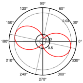
(b)

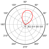
(c)

Figure 1: (a) The $Q$ function for the values $\alpha=2,r=0.7,\vartheta=0,\Delta=0.15\;\omega,\lambda=0.04\;\omega,\epsilon=1.3\;\omega,\mathrm{c}=1$ at scaled time $\omega t=30414$ using the (blue dashed) series evaluation (2.33), and the corresponding value (red solid) based on the linear approximation (2.35). The polar plot of the quadrature variance $V_{\varphi}$ (Sec. II E) is given in (b) for the said parameters. (c) The angular Husimi density $Q(\theta)$ on the phase space is plotted for the above set of parameters.

The functional form of $\Phi(\varpi,\mathsf{w},t)$ in (2.36) suggests that the superposition of Fourier modes leads to time-dependent frequencies of oscillation. The deviation between the series evaluation (2.33) and its approximation (2.35) may be measured via the following modulus:

$$||\delta Q||=\int|Q-Q_{{}_{\mathrm{linear}}}|\,\mathrm{d}^{2}\beta.$$ (2.37)

For the set of parameters specified in Fig. 1 its value $||\delta Q||=0.0214$ specify a $2\%$ error in estimation.

The angular Husimi density $Q(\theta)$ on the phase space [[41]] is useful in the study of the multiple peaks characterizing kitten-type of states:

$$Q(\theta)=\int_{0}^{\infty}Q(\beta,\beta^{*})|\beta|\,\mathrm{d}|\beta|,\quad\beta=|\beta|\exp(i\theta).$$ (2.38)

The positive semi-definite angular density is read off the Fourier mode expansion (2.32):

$$Q(\theta) = \!\!\frac{1}{\pi(1+|\mathrm{c}|)^{2}}\!\!\sum_{n,m=0}^{\infty}\!\!\;\mathcal{S}_{n}(\alpha_{+},\xi)\mathcal{S}_{m}(\alpha_{+},\xi)^{*}\left\lgroup\mathsf{C}_{n}(t)\mathsf{C}_{m}(t)^{*}\,\mathcal{H}_{n,m}^{(+)}(\theta)\right.$$ (2.39)

$$\quad+\;(-1)^{n+m}\mathsf{D}_{n}(t)\mathsf{D}_{m}(t)^{*}\,\mathcal{H}_{n,m}^{(-)}(\theta)\left.\right\rgroup\exp(-i(n-m)\omega t),$$

where mode sums of the hypergeometric series read:

$$\mathcal{H}_{n,m}^{(\pm)}(\theta) = \sum_{\jmath=0}^{n}\sum_{\ell=0}^{m}\binom{n}{\jmath}\binom{m}{\ell}\Big{(}\pm\dfrac{\lambda}{\omega}\Big{)}^{n+m-\jmath-\ell}\exp(-i\theta(\jmath-\ell))\exp\Big{(}-\dfrac{\lambda^{2}}{\omega^{2}}\sin^{2}\theta\Big{)}\times$$ (2.40)

$$\times\left\lgroup\dfrac{1}{2}\;\Gamma\Big{(}\dfrac{\jmath+\ell}{2}+1\Big{)}{}_{1}F_{1}\left(\begin{matrix}-(\jmath+\ell+1)/2\\ 1/2\end{matrix};-\frac{\lambda^{2}}{\omega^{2}}\cos^{2}\theta\right)\right.$$

$$\mp\,\left.\dfrac{\lambda}{\omega}\cos\theta\;\Gamma\Big{(}\dfrac{\jmath+\ell+3}{2}\Big{)}{}_{1}F_{1}\left(\begin{matrix}-(\jmath+\ell)/2\\ 3/2\end{matrix};-\frac{\lambda^{2}}{\omega^{2}}\cos^{2}\theta\right)\right\rgroup.$$

As an example we plot the angular density $Q(\theta)$ for the observed single-peak in Fig. 1 (c).

D. The angular distribution on the phase space

A quantity that directly measures the angular distribution on the phase space corresponding to the oscillator reduced density matrix (2.7) is given by [[44, 45]]

$$\mathcal{P}(\theta)=\frac{1}{2\pi}\langle\theta|\rho_{\mathcal{O}}|\theta\rangle,\quad|\theta\rangle=\sum_{n=0}^{\infty}\exp(in\theta)\,|n\rangle,$$ (2.41)

The states $|\theta\rangle$ are nonnormalizable and nonorthogonal for distinct values of the phase angle $\theta$. These states, however, provide the resolution of unity in the oscillator Hilbert space: $\frac{1}{2\pi}\int_{0}^{2\pi}\mathrm{d}\theta\,|\theta\rangle\langle\theta|=\mathbb{I}$. The definition (2.41) via the diagonal element of the density matrix imparts the following properties on the angular distribution function $\mathcal{P}(\theta)$:

$$\mathcal{P}(\theta)\geq 0,\quad\int_{0}^{2\pi}\mathcal{P}(\theta)\,\mathrm{d}\theta=1.$$ (2.42)

The oscillator reduced density matrix quoted in (2.8) now produces the angular density function as a nonnegative quantity:

$$\mathcal{P}(\theta)=\dfrac{1}{2\pi(1+|\mathrm{c}|^{2})}\Big{(}|\mathsf{X}(\theta,t)|^{2}+|\mathsf{Y}(\theta,t)|^{2}\Big{)},$$ (2.43)

where the Fourier sums may be listed as follows:

$$\mathsf{X}(\theta,t) = \sum_{n,k=0}^{\infty}(-1)^{k}\mathcal{S}_{n}(\alpha_{+},\xi)\,\mathsf{C}_{n}(t)\mathcal{G}_{n,k}(\sqrt{x}/2)\,\exp(-i(n\omega t+k\theta)),$$

$$\mathsf{Y}(\theta,t) = \sum_{n,k=0}^{\infty}\mathcal{S}_{n}(\alpha_{+},\xi)\,\mathsf{D}_{n}(t)\mathcal{G}_{n,k}(\sqrt{x}/2)\,\exp(-i(n\omega t+k\theta)).$$ (2.44)

The normalization relation (2.42) of the angular density (2.43) may be explicitly checked via the following identity [[50]] that reflects the orthonormality of the Charlier polynomials:

$$\sum_{k=0}^{\infty}\frac{\mathsf{t}^{k}}{k!}\;{}_{2}F_{0}\left(\begin{matrix}-n,-k\\ \underline{\phantom{x}}\end{matrix};-\frac{1}{\mathsf{t}}\right){}_{2}F_{0}\left(\begin{matrix}-k,-m\\ \underline{\phantom{x}}\end{matrix};-\frac{1}{\mathsf{t}}\right)=n!\;\mathsf{t}^{-n}\exp(\mathsf{t})\;\delta_{nm}.$$ (2.45)

The plots of the angular density distribution $\mathcal{P}(\theta)$ for the kitten states observed at the short time oscillations are given in Fig. 3.

E. The variance of the quadrature variables

While comparing between the phase space distributions associated with distinct density matrices the first and second moments of the quadrature variable

$$X_{\varphi}=\dfrac{1}{\sqrt{2}}(a\exp(-i\varphi)+a^{\dagger}\exp(i\varphi))$$ (2.46)

play an important role. The coordinate and the momentum operators are, respectively, given by $\mathsf{q}\equiv\frac{1}{\sqrt{2}}(a+a^{\dagger})=X_{0},\mathsf{p}\equiv\frac{1}{\sqrt{2}\,i}(a-a^{\dagger})=X_{\frac{\pi}{2}}$. Utilizing our explicit derivation (2.32) of the $Q(\beta,\beta^{*})$-function the expectation values of the said moments may be obtained:

$$\langle X_{\varphi}\rangle \equiv \hbox{Tr}(X_{\varphi}\rho_{\cal O}(t))=\dfrac{1}{\sqrt{2}}\int(\beta\exp(-i\varphi)+\beta^{*}\exp(i\varphi))Q(\beta,\beta^{*})\mathrm{d}^{2}\beta,$$

$$\langle X_{\varphi}^{2}\rangle \equiv \hbox{Tr}(X_{\varphi}^{2}\rho_{\cal O}(t))=\dfrac{1}{2}\int\Big{(}(\beta\exp(-i\varphi)+\beta^{*}\exp(i\varphi))^{2}-1\Big{)}Q(\beta,\beta^{*})\mathrm{d}^{2}\beta.$$ (2.47)

These expectation values read:

$$\langle X_{\varphi}\rangle = \frac{\sqrt{2}}{1+|\mathrm{c}|^{2}}\left\lgroup\mathrm{Re}\left(\sum_{n=0}^{\infty}\sqrt{n+1}\;G_{n,1}^{-}(\varphi,t)\right)-\frac{\sqrt{x}}{2}\,\cos\varphi\,\sum_{n=0}^{\infty}G_{n,0}^{-}(\varphi,t)\right\rgroup,$$ (2.48)

$$\langle X_{\varphi}^{2}\rangle = \dfrac{1+x\cos^{2}\varphi}{2}+|\alpha_{+}|^{2}+|\nu|^{2}+\frac{1}{1+|\mathrm{c}|^{2}}\mathrm{Re}\left\lgroup\sum_{n=0}^{\infty}\sqrt{(n+1)(n+2)}\;\times\right.$$ (2.49)

$$\times\left.\;G_{n,2}^{+}(\varphi,t)-2\sqrt{x}\,\cos\varphi\,\sum_{n=0}^{\infty}\sqrt{n+1}\;G_{n,1}^{+}(\varphi,t)\right\rgroup,$$

where we employ the following notations for the coefficients:

$$G_{n,\ell}^{\pm}(\varphi,t)=\mathcal{S}_{n}(\alpha_{+},\xi)\mathcal{S}_{n+\ell}(\alpha_{+},\xi)^{*}\;\Big{(}{\mathsf{C}_{n}}(t)\mathsf{C}_{n+\ell}(t)^{*}\pm\mathsf{D}_{n}(t){\mathsf{D}_{n+\ell}}(t)^{*}\Big{)}\;\exp(i\ell(\omega t+\varphi)).$$ (2.50)

To compute the moment (2.49) the following bilinear kernel of the Hermite polynomials has been used [[52]]:

$$\sum_{n=0}^{\infty}\dfrac{\mathrm{H}_{n}(\mathsf{w})\mathrm{H}_{n}(\mathsf{z})}{2^{n}n!}\mathsf{t}^{n}=\dfrac{1}{\sqrt{1-\mathsf{t}^{2}}}\exp\Big{(}\frac{2\mathsf{t}\mathsf{w}\mathsf{z}-\mathsf{t}^{2}(\mathsf{w}^{2}+\mathsf{z}^{2})}{1-\mathsf{t}^{2}}\Big{)}.$$ (2.51)

The variance $V_{\varphi}=\langle X_{\varphi}^{2}\rangle-\langle X_{\varphi}\rangle^{2}$ of the quadrature variable is minimized at an angle $\varphi_{\mathrm{min}}$ given by $\frac{\partial V_{\varphi}}{\partial\varphi}|_{{\varphi}_{\mathrm{min}}}=0,\frac{\partial^{2}V_{\varphi}}{\partial^{2}\varphi}|_{{\varphi}_{\mathrm{min}}}>0$. Its explicit value reads:

$$\varphi_{\mathrm{min}}=\frac{1}{2}\Big{(}\tan^{-1}\Big{(}\dfrac{\mathrm{Im}\langle(\Delta a)^{2}\rangle}{\mathrm{Re}\langle(\Delta a)^{2}\rangle}\Big{)}\pm\pi\Big{)},\quad\langle(\Delta a)^{2}\rangle\equiv\hbox{Tr}(\rho_{\cal O}(t)a^{2})-(\hbox{Tr}(\rho_{\cal O}(t)a))^{2}.$$ (2.52)

The state is squeezed along the $X_{\varphi_{\mathrm{min}}}$ quadrature, and stretched along the conjugate direction $\varphi_{\mathrm{min}}+\pi/2$ in the phase space. The polar plot of the variance $V_{\varphi}$ for a set of parameters is provided in Fig. 1 (b), where the minimum value of $V_{\varphi}$ reads 0.23, and the corresponding polar angle equals $\varphi=76.16^{\circ}$. We now list the time evolution of the first and the second moments of the quadrature variables [[53]] as follows:

$$\langle\mathsf{q}\rangle = \langle X_{0}\rangle,\langle\mathsf{p}\rangle=\langle X_{\frac{\pi}{2}}\rangle,\sigma_{11}\equiv\langle\mathsf{q}^{2}\rangle-\langle\mathsf{q}\rangle^{2}=\langle X^{2}_{0}\rangle-\langle X_{0}\rangle^{2},\sigma_{22}\equiv\langle\mathsf{p}^{2}\rangle-\langle\mathsf{p}\rangle^{2}=\langle X^{2}_{\tfrac{\pi}{2}}\rangle-\langle X_{\frac{\pi}{2}}\rangle^{2},$$

$$\!\!\sigma_{12}\!\!\!\! \equiv \!\!\!\!\!\!\dfrac{\langle(\mathsf{qp+pq})\rangle}{2}\!-\!\langle\mathsf{q}\rangle\langle\mathsf{p}\rangle\!\!=\!\dfrac{1}{1+|\mathrm{c}|^{2}}\mathrm{Im}\!\!\left\lgroup\!\sum_{n=0}^{\infty}\!\sqrt{n+1}\!\left(\sqrt{x}\;G_{n,1}^{+}(0,t)-\sqrt{n+2}\;G_{n,2}^{+}(0,t)\!\right)\!\!\right\rgroup\!\!\!-\!\!\langle X_{0}\rangle\langle X_{\frac{\pi}{2}}\rangle.$$ (2.53)

The quadrature moments (2.53) of the time-evolving oscillator states are used in Sec. III B towards characterizing their nonclassical properties.

III Kitten states in the presence of multiple time scales

The evolution (2.8) of the oscillator density matrix $\rho_{\mathcal{O}}(t)$ induces transient appearances of squeezed kitten states in the phase space for a strong coupling limit: $\lambda\lessapprox 0.1\,\omega$. The Wehrl entropy [[38]] has been used [[41]] as an important tool for providing the description of these states. Defined as

$$S_{Q}=-\int\,Q(\beta,\beta^{*})\,\log Q(\beta,\beta^{*})\,\mathrm{d}^{2}\beta,$$ (3.1)

it measures the delocalization of the system in the oscillator phase space, and is considered as a count of an equivalent number of widely separated coherent states necessary for tiling the existent occupation on the phase space [[54]]. As the averaging process via a Gaussian kernel (2.30) plays a key role in the construction of the nonnegative $Q$-function, the Wehrl entropy (3.1) may be envisaged as a quasi classical coarse grained analog [[55]] of the quantum von Neumann entropy $S$. In the context of the nonlinear self-interacting Kerr type photonic models, the unitary time evolution of a pure coherent state has been found [[39]-[42]] to lead to the formations of the transient kitten states characterized by the superposition of a finite number of macroscopic coherent states. In the interaction picture the nonlinearity engenders a periodicity of the Wehrl entropy $S_{Q}$ that develops a series of local minima at the rational submultiples of the said time period. Owing to the presence of the interference terms, these superposition of multiple coherent states are nonclassical in nature. Recently the experimental realization [[24]] of these kitten states has been established. The emergence of these transitory kitten states in the bipartite qubit-oscillator interacting model studied here has been briefly observed earlier [[56]]. In the current section we provide a detailed investigation of this issue.

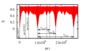
(a)

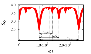
(b)

Figure 2: The long time quasi periodic behavior with the time period $T_{\hbox{\tiny{long}}}\sim O((x^{2}\widetilde{\Delta})^{-1})$ is observed for (a) the von Neumann entropy $S$, and (b) the Wehrl entropy $S_{Q}$ for the parametric values $\alpha=3,r=0.7,\vartheta=0,\Delta=0.15\;\omega,\lambda=0.05\;\omega,\epsilon=0,\mathrm{c}=i$. The semiclassical Wehrl entropy $S_{Q}$ faithfully reproduces periodicity and the local minima structure of the quantum entropy $S$, even though the quantum fluctuations due to a multiplicity of modes originating due to the interaction are more prominent for the latter. The above parameters produce the time period $\omega T_{\hbox{\tiny{long}}}$ = 1730000.

In the coupling domain $\lambda\lessapprox 0.1\,\omega$ the interaction frequencies $O(x^{2}\widetilde{\Delta})$ and their harmonics are activated giving rise to a long time quasi periodic behavior: $T_{\hbox{\tiny{long}}}\sim O((x^{2}\widetilde{\Delta})^{-1})$. In Fig. 2 we observe this quasi periodicity in the evolution of both the quantum von Neumann entropy $S$, and the quasi classical Wehrl entropy $S_{Q}$. The emergence of the long time quasi periodicity, and the occurrence of the local minima at the rational submultiples of $T_{\hbox{\tiny{long}}}$ are identically realized for both $S$ (Fig. 2 (a)), and $S_{Q}$ (Fig. 2 (b)). The quantum fluctuations generated by an array of modes are, however, more evident in the entropy $S$ rather than in its coarse grained analog $S_{Q}$. Moreover, the existence of particularly low values of the entropy $S$ during its time evolution points towards the briefly emerging almost pure states of the oscillator subsystem. In contrast to the nonlinear self-interacting Kerr type of models, the qubit-oscillator interaction studied here induces a variety of incommensurate modes reflecting a multiplicity of dynamically activated interaction-dependent time scales. In the coupling range $\lambda\lessapprox 0.1\,\omega$, the modes of frequencies $O(x\widetilde{\Delta})$ cause short range oscillations superimposed on the long time quasi periodic behavior observed earlier. In particular, these linear modes originating via the qubit-oscillator interaction induce an energy transfer between the constituent degrees of freedom in a short time scale. In the vicinity of the instants marked as the rational submultiples of $T_{\hbox{\tiny{long}}}$ the phase space occupation, modulo the fluctuations caused by the modes with frequencies $O(x\widetilde{\Delta})$, achieves a local minimum. The short time period quantum fluctuations, however, necessitate spreading on the phase space by splitting the Gaussian peaks (Fig. 3, columns 2, 4) when the energy transfers from the qubit to the oscillator mode. The splitting and subsequent rejoining of the Gaussian peaks produced by the interacting modes with frequencies $O(x\widetilde{\Delta})$ cause the local fluctuations in the Wehrl entropy $S_{Q}$ and other dynamical quantities. The splitting of the kittens in the phase space indicates rapidly growing internal complexity of the state in the timescale $O((x\widetilde{\Delta})^{-1})$, and is associated with a concomitant growth of entropies $(S,S_{Q})$. We investigate these issues with the choice of the coefficient $\mathrm{c}=i$ in the initial hybrid state (2.2) as its time evolution offers the possibility of creating relatively pure Yurke-Stoler type [[57]] of squeezed states with sufficiently high fidelity. As evident in the behavior of the entropies ($S,S_{Q}$) in Fig. 2, the relative phase $\mathrm{c}=i$ in the state (2.2) causes an initial time translation, compared to the $\mathrm{c}=\pm 1$ cases, by the amount $T_{\hbox{\tiny{long}}}/2$.

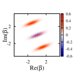
(a)

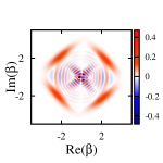
(b)

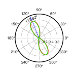
(c)

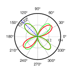
(d)

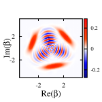
(e)

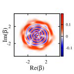
(f)

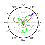
(g)

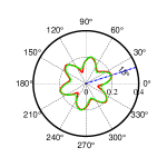
(h)

(i)

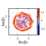
(j)

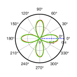
(k)

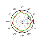
(l)

Figure 3: The Wigner $W$-distribution (columns $1,2$) and the polar plot for $\mathcal{P}(\theta)$ (columns $2,4$) at times, equivalent up to a period, $T_{\hbox{\tiny{long}}}/2$ (row $1$), $T_{\hbox{\tiny{long}}}/3$ (row $2$), and $T_{\hbox{\tiny{long}}}/4$ (row $3$) respectively. The parameters are chosen as $\alpha=3,r=0.7,\vartheta=0,\Delta=0.15\,\omega,\lambda=0.05\,\omega,\epsilon=0,\mathrm{c}=i$. The short time fluctuations of frequencies $O(x\widetilde{\Delta})$ superposed on the quadratic $T_{\hbox{\tiny{long}}}$ modes cause the entropies ($S,S_{Q}$) to achieve a local minimum and a neighboring maximum at times $\omega t=2205$ and $\omega t=3371$ (for $T_{\hbox{\tiny{long}}}/2$), $\omega t=287055$ and $\omega t=286370$ (for $T_{\hbox{\tiny{long}}}/3$), $\omega t=435013.2$ and $\omega t=434450$ (for $T_{\hbox{\tiny{long}}}/4$), respectively. At the minima of the short time fluctuations at $T_{\hbox{\tiny{long}}}/p$ give rise to $p$ kitten states that bifurcate into $2p$ kitten states at the adjacent maxima arrived at the short time scale $T_{\hbox{\tiny{short}}}$. The green dotted lines in column 3 (4) depict the phase space angular density $\mathcal{P}(\theta)$ of the reference state (3.2) ((3.11)) with the choice of parameters given in Table 1 (2).

In Fig. 3 we plot the Wigner $W$-distribution and the angular phase space density $\mathcal{P}(\theta)$ at times that, up to a period $T_{\hbox{\tiny{long}}}$, are identical with the rational submultiples $T_{\hbox{\tiny{long}}}/2,T_{\hbox{\tiny{long}}}/3,T_{\hbox{\tiny{long}}}/4$, respectively. The geometry of the domain on the phase space supporting the $W$-distribution comprises of the Gaussian peaks and their intermediate zones containing the interference pattern that exhibits oscillations in a direction perpendicular to the line joining the peaks. As a signature of strong nonclassicality of the state significantly large negative domains in the $W$-distribution appear. The short time oscillations of frequency $O(x\widetilde{\Delta})$ are manifest in Fig. 3 as its columns $1$ and $3$ ($2$ and $4$) refer, respectively, to the $W$-distribution and the polar density plot $\mathcal{P}(\theta)$ to the minimum (maximum) configuration of the quasi classical Wehrl entropy $S_{Q}$. The bifurcation and rejoining of the Gaussian peaks at the time scale $T_{\hbox{\tiny{short}}}\sim O((x\widetilde{\Delta})^{-1})$ are clearly evident in these diagrams. Here we make a comment on our selection of the coefficient $\mathrm{c}=i$ described above. Generally speaking, this choice leads to lower entropy states than, say, for alternative values such as $\mathrm{c}=\pm 1$. Moreover, in the former case the odd kitten states $(p=1,3,\ldots)$ are produced for all values of the bias $\epsilon$, whereas in the latter case odd kitten states are realized only for high $\epsilon$. This follows from the symmetry $Q(\beta,\beta^{*})|_{\epsilon=0}=Q(-\beta,-\beta^{*})|_{\epsilon=0}$ for $\mathrm{c}=\pm 1$ as evident in (2.32). One effect of having a high bias parameter ($\epsilon\sim\omega$) is that the number of participant interaction-dependent modes will increase much, causing wider fluctuations in the observed dynamical quantities.

We now attempt (Fig. 4) a more detailed description of the splitting and rejoining of the kitten states in the phase space at time scale $T_{\hbox{\tiny{short}}}$. The columns (a), (b), and (c) in Fig. 4 refer, respectively, to the evolution of the physical quantities close to the rational submultiples $T_{\hbox{\tiny{long}}}/2,T_{\hbox{\tiny{long}}}/3,T_{\hbox{\tiny{long}}}/4$ of the long period. In the rows $1,2,3$ and $4$ of Fig. 4 we plot the time evolution at the scale $T_{\hbox{\tiny{short}}}$ of the Wehrl entropy $S_{Q}$, entropy $S$, negativity $\delta_{W}$, and the Hilbert-Schmidt distance $d_{\mathrm{HS}}$ between quantum states, respectively. In specific, we attempt to reconstruct the states where the quantum entropy $S$ dips to particularly low values signaling evolution to states which are close to pure states of the oscillator subsystem. Moreover, towards establishing the nonclassical nature of the maximum entropy ($S$) states realized at the time scale $T_{\hbox{\tiny{short}}}$, we compare them with the most general statistical mixture of states possessing nonnegative $W$-distribution, but, nonetheless, endowed with a parallel configuration of Gaussian peaks in the phase space.

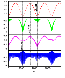
(a)

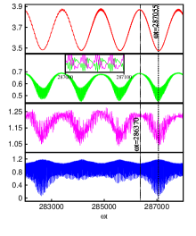
(b)

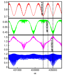
(c)

Figure 4: We plot the short time $O(x\widetilde{\Delta})$ fluctuations of the Wehrl entropy $S_{Q}$(red), von Neumann entropy $S$(green), negativity $\delta_{W}$(magenta), and the Hilbert-Schmidt distance $d_{\mathrm{HS}}(\rho_{\mathcal{O}}(t),\rho_{\mathcal{O}}({t_{{\mathrm{ref}}}}))$(blue) at times (equivalent up to a period $T_{\hbox{\tiny{long}}}$) $T_{\hbox{\tiny{long}}}/2$ (column $1$), $T_{\hbox{\tiny{long}}}/3$ (column $2$), and $T_{\hbox{\tiny{long}}}/4$ (column $3$) respectively. The chosen parametric values read: $\alpha=3,r=0.7,\vartheta=0,\Delta=0.15\,\omega,\lambda=0.05\,\omega,\epsilon=0,\mathrm{c}=i$. Towards calibrating the Hilbert-Schmidt distance $d_{\mathrm{HS}}(\rho_{\mathcal{O}}(t),\rho_{\mathcal{O}}({t_{{\mathrm{ref}}}}))$ between the quantum states, we, in Figs. (a, b, c), have chosen the reference times $\omega t_{\mathrm{ref}}$ as $2205,287055,435013.2$, respectively.

A. Reconstructing states at the minimum entropy regime

The minima realized during the short time oscillations of the Wehrl entropy $S_{Q}$ with frequencies $O(x\widetilde{\Delta})$ at the time limits $T_{\hbox{\tiny{long}}}/p,$ where $p=2,3,\ldots$, are associated with $p$ kitten states as evident from the corresponding Wigner $W$-distribution (Fig. 3, column $1$) and the angular phase density $\mathcal{P}(\theta)$ (Fig. 3, column $3$). We note that, among the quantities $(S_{Q},S,\delta_{W},d_{\mathrm{HS}})$ studied in Fig. 4, the time variation of the Wehrl entropy $S_{Q}$ (Fig. 4, row $1$) obtained via the smoothed phase space quasiprobability $Q$-function is not replicated, in general, by the other variables carrying more quantum informations. For instance, say for the $p=2,4$ cases the entropy $S$ (Fig. 4, row $2$) possesses domains of its near maximal values even in the regions where the quasi classical quantity $S_{Q}$ is at its minimum. But, interestingly, a local minimum in the entropy $S$ among the adjoining states develop corresponding to a minimum of its quasi classical analog $S_{Q}$. This feature, where the entropy $S$ undergoes a tiny dip in its value, may be noticed at $\omega t=4410$ for $p=2$ (Fig. 4 (a)), and $\omega t=433910.5$ for $p=4$ (Fig. 4 (c)), respectively. A minimum entropy ($S$) configuration indicates relative closeness to a pure state in the Hilbert space, and, in general, a consequent decrease in the statistical mixedness of the density matrix. The increase in the quantum nature of the state results in a consequent enhancement in negativity $\delta_{W}$ relative to the neighboring states, as observed in Fig. 4 (a) at time $\omega t=2205$, and at the inset in Fig. 4 (b) between the time span $\omega t=287000$ and $\omega t=287100$. However, we observe that the Hilbert-Schmidt distance $d_{\mathrm{HS}}$ (Fig. 4, row $4$) between the density matrices most faithfully distinguishes between the quantum states. The distance $d_{\mathrm{HS}}$ between the quantum states (2.12) are evaluated from the pertinent fiducial states marked in the diagram: $\omega t=2205$ for $p=2$ (Fig. 4 (a)), $\omega t=287055$ for $p=3$ (Fig. 4 (b)), and $\omega t=435013.2$ for $p=4$ (Fig. 4 (c)). In the above cases we notice that the distance $d_{\mathrm{HS}}$ between the time-evolving oscillator state and the pertinent reference marker state approaches a null value only after a full rotation by the angle $2\pi$ on the complex plane i.e. after completing $p$ cycles in the fluctuations of the Wehrl entropy $S_{Q}$ with the period $T_{\hbox{\tiny{short}}}$.

We now employ the distance $d_{\mathrm{HS}}$ between the density matrices to determine the proximity of the oscillator density matrix (2.8) at the above low entropy ($S$) limits to the pure states comprising appropriately rotated and equi-separated $p$ kitten states in the phase space. To facilitate this reconstruction of a given state we use an ensemble of density operators that represent a weighted combination of (a) a dominant pure state reflecting the said superposition of $p$ kitten states, as well as (b) a comparatively weaker statistical mixture of the density matrices of these individual $p$ kitten states. The second term measures the small departure of the state (2.8) from a pure $p$-kitten state density matrix at the chosen times. The construction of the ensemble of the reference states reads:

$$\widetilde{\rho}=\tau\rho_{{}_{\mathrm{pure}}}+(1-\tau)\rho_{{}_{\mathrm{mixed}}},$$ (3.2)

where the pure state represents a quantum superposition of $p$ equally separated squeezed kitten states:

$$\rho_{{}_{\mathrm{pure}}}=|\psi\rangle\langle\psi|,\quad|\psi\rangle=\dfrac{1}{\sqrt{N_{{}_{\mathrm{pure}}}}}\sum_{k=0}^{p-1}f_{k}|\alpha_{k},\xi_{k}\rangle,\;N_{{}_{\mathrm{pure}}}=\sum_{k,\ell=0}^{p-1}f_{k}f_{\ell}^{*}\langle\alpha_{\ell},\xi_{\ell}|\alpha_{k},\xi_{k}\rangle,$$ (3.3)

and the mixed state constitutes a statistical mixture of the density matrices of the above squeezed coherent states:

$$\rho_{{}_{\mathrm{mixed}}}=\dfrac{1}{N_{{}_{\mathrm{mixed}}}}\sum_{k=0}^{p-1}g_{k}|\alpha_{k},\xi_{k}\rangle\langle\alpha_{k},\xi_{k}|,\quad N_{{}_{\mathrm{mixed}}}=\sum_{k=0}^{p-1}g_{k}.$$ (3.4)

The phase space coordinates and the squeezing parameters of the $p$ squeezed coherent states employed for the above reconstruction process read:

$$\alpha_{k}=\alpha_{+}\exp(i(\widetilde{\vartheta}+2\pi k/p))\quad\xi_{k}=\xi\exp(2i(\widetilde{\vartheta}+2\pi k/p)),\quad\nu_{k}=\nu\exp(2i(\widetilde{\vartheta}+2\pi k/p)),$$ (3.5)

where the supplementary angle of rotation $\widetilde{\vartheta}$ has been introduced for implementing maximum phase space overlap between the density matrix of the reference state (3.2) and that of the transient squeezed kitten states of the density matrix (2.8) observed when the low entropy configurations at $T_{\hbox{\tiny{long}}}/p$ are realized. This is explicitly determined from the angular distribution function $\mathcal{P}(\theta)$ for the respective cases. The angular distribution $\mathcal{P}(\theta)$ of the fiducial state (3.2) are marked in green dotted lines in the Figs. 3 (c, g, k) with the choice of the initial angle $\widetilde{\vartheta}$ and other parameters given in Table 1. In these cases the angular distribution functions $\mathcal{P}(\theta)$ of the two density matrices in comparison make complete overlap. The $\mathcal{P}(\theta)$ function for the density matrix (3.2) may be easily calculated. We have not explicitly reproduced it here. The inner product of the squeezed coherent states used in constructing the density matrix (3.2) may be given as below:

$$\langle\alpha_{\ell},\xi_{\ell}|\alpha_{k},\xi_{k}\rangle=\dfrac{1}{\sqrt{\mu^{2}-\nu_{k}\nu_{\ell}^{*}}}\exp\Big{(}-\dfrac{{\mathsf{N}}_{k\ell}}{\mu^{2}-\nu_{k}\nu_{\ell}^{*}}\Big{)},$$ (3.6)

where the exponent reads

$${\mathsf{N}}_{k\ell}=|\alpha_{+}|^{2}(\mu^{2}+\nu_{k}\nu_{\ell}^{*})-\alpha_{k}\alpha_{\ell}^{*}(\mu^{2}+|\nu|^{2})+\dfrac{\mu\nu_{k}}{2}(\alpha_{k}^{*}-\alpha_{\ell}^{*})^{2}+\dfrac{\mu\nu_{\ell}^{*}}{2}(\alpha_{k}-\alpha_{\ell})^{2}.$$ (3.7)

The equality (2.25) allows us to evaluate the Hilbert-Schmidt distance $d_{\mathrm{HS}}$ between two density matrices via the corresponding Wigner $W$-distributions. Towards this end we now produce the $W$-distribution of the ensemble of the fiducial state (3.2) as follows:

$$\widetilde{W}(\beta,\beta^{*})=\tau\;\dfrac{1}{N_{{}_{\mathrm{pure}}}}\sum_{k,\ell=0}^{p-1}f_{k}f_{\ell}^{*}\;\widetilde{W}_{k\ell}(\beta,\beta^{*})+(1-\tau)\;\dfrac{1}{N_{{}_{\mathrm{mixed}}}}\sum_{k=0}^{p-1}g_{k}\;\widetilde{W}_{kk}(\beta,\beta^{*}),$$ (3.8)

where the component $\widetilde{W}_{k\ell}(\beta,\beta^{*})$ associated with the projection operator $|\alpha_{k},\xi_{k}\rangle\langle\alpha_{l},\xi_{l}|$ may be determined à la the series sum given in (2.19):

$$\widetilde{W}_{k\ell}(\beta,\beta^{*})=\dfrac{2}{\pi}\sum^{\infty}_{n=0}(-1)^{n}\langle\beta,n|\alpha_{k},\xi_{k}\rangle\langle\alpha_{\ell},\xi_{\ell}|\beta,n\rangle=\dfrac{2}{\pi\sqrt{\mu^{2}-\nu_{k}\nu_{\ell}^{*}}}\;\exp\Big{(}-\dfrac{{\mathsf{N}}_{k\ell}+2{\mathsf{G}}_{k\ell}}{\mu^{2}-\nu_{k}\nu_{\ell}^{*}}\Big{)},$$ (3.9)

where the Gaussian exponent is given by

$${\mathsf{G}}_{k\ell}=\mu^{2}(\alpha_{k}-\beta)(\alpha_{\ell}^{*}-\beta^{*})+\nu_{k}\nu_{\ell}^{*}(\alpha_{k}^{*}-\beta^{*})(\alpha_{\ell}-\beta)+\,\mu\nu_{k}(\alpha_{k}^{*}-\beta^{*})(\alpha_{\ell}^{*}-\beta^{*})+\mu\nu_{\ell}^{*}(\alpha_{k}-\beta^{)}(\alpha_{\ell}-\beta).$$ (3.10)

Following the above procedure we now attempt an explicit reconstruction of the density matrices associated with the transient kitten states as the candidates located in the Hilbert space in close neighborhood of the corresponding pure states (3.3). To illustrate the process we choose the following examples at times (i) $\omega t=2205$ in Fig. 4 (a), (ii) $\omega t=287055$ (Fig. 4 (b)), and (iii) $\omega t=435013.2$ (Fig. 4 (c)), where the entropy $S$ assumes a local minimum value regarding the fluctuations in the time scale $T_{\hbox{\tiny{short}}}$. The parameters defining the fiducial marker state (3.2) $\{f_{k},g_{k}|k=0,1,\ldots,p-1;\tau\}$ are varied independently to obtain the minimum Hilbert-Schmidt distance between the density matrices $\rho_{\mathcal{O}}$ and $\widetilde{\rho}$. Even though the decomposition process (3.2) and the subsequent reconstruction of the density matrix are not unique, but the variational computation based on minimization of the Hilbert-Schmidt distance provides a robust selection process in a large ensemble of states. The results are summarized in Table 1. We express our results in terms of a dimensionless quantity maintaining values $d_{\mathrm{HS}}(\rho_{\mathcal{O}}(t),\widetilde{\rho})/\sqrt{\mathrm{Tr}(\rho_{\mathcal{O}}(t)^{2})}\ll 1$ at times when the low entropy states are realized. The margin of error in the above analysis is limited by the requirement $\Delta d_{\mathrm{HS}}(\rho_{\mathcal{O}}(t),\widetilde{\rho})\leq|d_{\mathrm{HS}}(\rho_{\mathcal{O}}(t),\widetilde{\rho})|$. The data presented in Table 1 suggest that as the number of kittens increases the maximum possible error is also increased. These examples, considered at the instants corresponding to locally minimum entropy $S$ configurations, indicate that, modulo a small component of statistical mixed state, the oscillator density matrix (2.8) evolves to a generalized Yurke-Stoler [[57]] type of pure state.

$\omega t$	$p$	$S$	$\widetilde{\vartheta}$	$f_{k}|k=0,1,\ldots,p-1$	$g_{k}|k=0,1,\ldots,p-1$	$\tau$	$d_{\mathrm{HS}}(\rho_{\mathcal{O}}(t),\widetilde{\rho})\;\;$	$\dfrac{d_{\mathrm{HS}}(\rho_{\mathcal{O}}(t),\widetilde{\rho})}{\sqrt{\mathrm{Tr}(\rho_{\mathcal{O}}(t)^{2}}}\;\;$
$2205$	2	0.0118	$112.82^{\circ}$	$1$, $\exp(i\pi 1.677)$	$1,1$	0.996	0.0647	0.0649
$\!\!\!\!\!287055$	3	0.4495	$40.1^{\circ}$	$1$, $0.97\exp(i\pi 1.315)$, $0.625\exp(i\pi 1.415)$	$0,0.095,1.275$	0.783	0.0879	0.1034
$\!\!\!\!\!434013.2$	4	$0.4085$	$0^{\circ}$	$1$, $0.96\exp(i\pi 0.11)$, $\exp(i\pi 1.005)$, $0.96\exp(i\pi 1.895)$	$1,1.54,1.14,1.50$	0.810	0.1467	0.1685

Table 1: Reconstruction of oscillator states in the neighborhood of pure states

B. Characterization of states at the large entropy regime

In Fig. 4 we observe that the quantum fluctuations of the frequencies $O(x\widetilde{\Delta})$ give rise to a periodic $(T_{\hbox{\tiny short}})$ maximization of the entropy $S$ and the Wehrl entropy $S_{Q}$. At the instants when the entropies are maximized, the $T_{\hbox{\tiny short}}$ fluctuations occurring at the long range time scales $T_{\hbox{\tiny long}}/p$ (up to a period $T_{\hbox{\tiny long}}$) produce, on account of the splitting in the phase space distribution, a combination of $2p\,(p=2,3,4,\ldots)$ squeezed kitten configurations. In particular, we examine the oscillator phase space distributions at times $\omega t=3371$ (Fig. 4 (a)), $\omega t=286370$ (Fig. 4 (b)), and $\omega t=434450$ (Fig. 4 (c)), which, as it is evident in the Fig. 3 (columns $2,4$), correspond to $4,6$, and $8$ squeezed kitten configurations, respectively, in the phase space. As these states possess large entropy ($S$), they are necessarily far away from the pure states in the Hilbert space. However, they are also endowed with large negativity $\delta_{W}$ (Fig. 4) of the Wigner $W$-distribution, and, consequently, they are strongly nonclassical in nature.

To study the non-Gaussian properties of the above states we compare them with the most general statistical mixture of the Gaussian squeezed states, where the ensemble exhibits an identical number of kitten configurations in the phase space. The density matrix of such a state with an array of equally separated $2p$ kitten combinations in the phase space is given by [[53]]

$$\rho_{{}_{\mathrm{mixed}}}^{\hbox{\tiny th}}=\dfrac{1}{N_{\mathrm{mixed}}}\sum_{k=0}^{2p-1}g_{k}\,\mathrm{D}(\alpha_{k})\mathrm{S}(\xi_{k})\rho_{{}_{\mathrm{th}}}\mathrm{S}^{\dagger}(\xi_{k})\mathrm{D}^{\dagger}(\alpha_{k}),\quad\rho_{{}_{\mathrm{th}}}=\dfrac{1}{\bar{n}+1}\,\left(\dfrac{\bar{n}}{\bar{n}+1}\right)^{a^{\dagger}a},\;\;\bar{n}=\dfrac{1}{\exp(\beta_{B}\omega)-1},$$ (3.11)

where $\rho_{{}_{\mathrm{th}}}$ is equilibrium thermal density matrix, and $\beta_{\mathrm{B}}$ is the inverse temperature. It has been proposed [[59]] that the zero temperature limit of the state (3.11) may be employed towards enhancing the upper bound on the accessible information in a Gaussian private quantum channel. The Wigner $W$-distribution of the Gaussian state (3.11) is nonnegative, and, therefore, it may be used as a suitable benchmark for studying the quantum features of the oscillator density matrix evolving in time. For later use we quote the quasi probability distributions of the statistical mixed state (3.11) below:

$$W(\beta,\beta^{*})|_{{}_{\mathrm{mixed}}} = \dfrac{1}{\pi(\bar{n}+1/2)\,N_{{}_{\mathrm{mixed}}}}\sum_{k=0}^{2p-1}\;g_{k}\exp\left\lgroup-\dfrac{1}{\bar{n}+1/2}|\mu(\alpha_{k}-\beta)+\nu_{k}(\alpha_{k}^{*}-\beta^{*})|^{2}\right\rgroup,$$ (3.12)

$$Q(\beta,\beta^{*})|_{{}_{\mathrm{mixed}}} = \dfrac{1}{\pi\,\mathfrak{N}\,N_{{}_{\mathrm{mixed}}}}\sum_{k=0}^{2p-1}\;g_{k}\exp\left\lgroup-\dfrac{1}{\mathfrak{N}^{2}}\Big{(}(\mu^{2}(1+\bar{n})+|\nu|^{2}\bar{n})|\beta-\alpha_{k}|^{2}\right.$$ (3.13)

$$+\left.\dfrac{\mu}{2}(2\bar{n}+1)(\nu_{k}^{*}(\beta-\alpha_{k})^{2}+\nu_{k}(\beta^{*}-\alpha_{k}^{*})^{2})\Big{)}\right\rgroup,\quad\mathfrak{N}=\sqrt{\bar{n}^{2}+\mu^{2}(2\bar{n}+1)}.$$

Towards examining the above mentioned high entropy states displaying nonclassicality vis a vis their Gaussian partners now we compute the first two moments of the quadrature variables with respect to the statistical mixture given in (3.11). The underlying idea is to distinguish between the non-Gaussian high entropy squeezed kitten state configurations, and the corresponding Gaussian states endowed with almost identical gross characteristics like the first two moments of the quadrature variables [[53]]. The expectation value of a dynamical observable for the Gaussian statistical mixture (3.11) reads: $\langle\mathcal{X}\rangle_{{}_{\mathrm{mixed}}}=\mathrm{Tr}(\mathcal{X}\rho_{{}_{\mathrm{mixed}}}^{\hbox{\tiny th}})$. As the moments up to the second order completely describe the Gaussian states, we quote them below:

$$\langle\mathsf{q}\rangle_{{}_{\mathrm{mixed}}} = \dfrac{\sqrt{2}}{N_{{}_{\mathrm{mixed}}}}\sum_{k=0}^{2p-1}\;g_{k}\;\mathrm{Re}(\alpha_{k}),\qquad\langle{\mathsf{p}}\rangle_{{}_{\mathrm{mixed}}}=\dfrac{\sqrt{2}}{N_{{}_{\mathrm{mixed}}}}\sum_{k=0}^{2p-1}\;g_{k}\;\mathrm{Im}(\alpha_{k}),$$

$$\langle\mathsf{q}^{2}\rangle_{{}_{\mathrm{mixed}}} = \dfrac{1}{N_{{}_{\mathrm{mixed}}}}\sum_{k=0}^{2p-1}\;g_{k}\left((\bar{n}+\tfrac{1}{2})(\mu^{2}+|\nu|^{2}-2\mu\,\mathrm{Re}(\nu_{k}))+2\left(\mathrm{Re}(\alpha_{k})\right)^{2}\right),$$

$$\langle\mathsf{p}^{2}\rangle_{{}_{\mathrm{mixed}}} = \dfrac{1}{N_{{}_{\mathrm{mixed}}}}\sum_{k=0}^{2p-1}\;g_{k}\left((\bar{n}+\tfrac{1}{2})(\mu^{2}+|\nu|^{2}+2\mu\,\mathrm{Re}(\nu_{k}))+2\left(\mathrm{Im}(\alpha_{k})\right)^{2}\right),$$

$$\tfrac{1}{2}\,\langle(\mathsf{p\,q+q\,p})\rangle_{{}_{\mathrm{mixed}}} = \dfrac{1}{N_{{}_{\mathrm{mixed}}}}\sum_{k=0}^{2p-1}\;g_{k}\;\mathrm{Im}\Big{(}\alpha_{k}^{2}-(2\bar{n}+1)\mu\,\nu_{k}\Big{)}.$$ (3.14)

The second order covariance matrix elements [[53]] for the state (3.11) are given by

$$\sigma_{11}|_{{}_{\mathrm{mixed}}} = \langle\mathsf{q}^{2}\rangle_{{}_{\mathrm{mixed}}}-\langle\mathsf{q}\rangle^{2}_{{}_{\mathrm{mixed}}},\quad\sigma_{22}|_{{}_{\mathrm{mixed}}}=\langle\mathsf{p}^{2}\rangle_{{}_{\mathrm{mixed}}}-\langle\mathsf{p}\rangle^{2}_{{}_{\mathrm{mixed}}},$$

$$\sigma_{12}|_{{}_{\mathrm{mixed}}} = \tfrac{1}{2}\,\langle(\mathsf{p\,q+q\,p})\rangle_{{}_{\mathrm{mixed}}}-\langle\mathsf{q}\rangle_{{}_{\mathrm{mixed}}}\,\langle\mathsf{p}\rangle_{{}_{\mathrm{mixed}}}.$$ (3.15)

$\omega t$	$2p$	$\begin{pmatrix}\langle\mathsf{q}\rangle\\ \langle\mathsf{p}\rangle\end{pmatrix}$	$\begin{pmatrix}\sigma_{11}\\ \sigma_{12}\\ \sigma_{22}\end{pmatrix}$	$\widetilde{\vartheta}$	$\!\!g_{k}|k=0,1,\ldots,2p-1\!\!\!\!$	$\begin{pmatrix}\langle\mathsf{q}\rangle\\ \langle\mathsf{p}\rangle\end{pmatrix}_{{}_{\!\!\!\mathrm{\!\!\!mixed}}}\!\!\!$	​​​$\!\!\!\begin{pmatrix}\sigma_{11}\\ \sigma_{12}\\ \sigma_{22}\end{pmatrix}_{{}_{\!\!\!\mathrm{\!\!\!mixed}\;\;}}\;\;$	$S(Q||Q_{{}_{\mathrm{mixed}}})\;\;$	$d_{\mathrm{HS}}(\rho_{\mathcal{O}},\rho_{{}_{\mathrm{mixed}}}^{\hbox{\tiny th}})\;\;$	$\dfrac{d_{\mathrm{HS}}(\rho_{\mathcal{O}},\rho_{{}_{\mathrm{mixed}}}^{\hbox{\tiny th}})}{\sqrt{\mathrm{Tr}(\rho_{\mathcal{O}}(t)^{2}}}\;\;$
3371	4	$-0.00062,$ $0$	$11.09$, $-0.10$, $9.67$	$\!\!\!135.22^{\circ}\;\;\;\;\;\;\;\;\;$	1.04081, 1.01542, 1.0404, 1.015	$-0.00062$, $0$	10.38, $-0.10$, 10.38	$0.0266$	0.518	0.732
286370	6	0.0083, 0.000012	10.36, 0.04, 10.38	$18^{\circ}$	0.9925, 1.02, 0.98139, 0.99, 1.014, 0.99129	0.0079, 0.000012	10.31, 0.04, 10.45	0.0025	0.583	0.818
434450	8	$-0.179,$ $-0.033$	10.30, $-0.05$, 10.38	$26.1^{\circ}$	0.986, 0.943, 1, 1, 1, 1.003, 1, 1	$-0.174$, $-0.034$	10.41, $-0.05$, 10.34	0.0049	0.604	0.832

Table 2: Non-Gaussian characteristics of the high entropy states

To emphasize the essential feature of nonclassicality that separates the oscillator state (2.8) at the above high entropy ($S$) configurations with the corresponding statistical mixture of the Gaussian states (3.11) we further obtain the Kullback-Leibler relative entropy [[58]] between their respective positive semidefinite $Q$-functions. Assuming that the Husimi $Q$-functions $(Q_{1}(\beta,\beta^{*}),Q_{2}(\beta,\beta^{*}))$ corresponding to their specific quantum density matrices $(\rho_{1},\rho_{2})$ are known, the nonnegative divergence between the two quasi probability distributions is defined as follows:

$$S_{\mathrm{KL}}(Q_{1}(\beta,\beta^{*})||Q_{2}(\beta,\beta^{*}))=\int Q_{1}(\beta,\beta^{*})\log\left(\dfrac{Q_{1}(\beta,\beta^{*})}{Q_{2}(\beta,\beta^{*})}\right)\mathrm{d}^{2}\beta.$$ (3.16)

The construction of the divergence between the two states may be thought of as the quasi classical analog of the quantum relative entropy $S(\rho_{1}||\rho_{2})=\mathrm{Tr}[\rho_{1}(\log\rho_{1}-\log\rho_{2})]$ [[60]] much in the sense that Wehrl entropy $S_{W}$ is regarded [[55]] a qualitatively similar approximation to the von Neumann entropy $S$. We make the identification of the oscillator $Q$-function (2.32) with $Q_{1}(\beta,\beta^{*})$ and that of the statistical mixed state (3.13) with $Q_{2}(\beta,\beta^{*})$.

The oscillator density matrix (2.8) corresponding to $2p$ squeezed kitten states with near-maximal entropy configuration arrived at times $T_{\hbox{\tiny long}}/p$ (up to a period $T_{\hbox{\tiny long}}$) is now compared with the fiducial density matrix (3.11). Employing the angular distribution function $\mathcal{P}(\theta)$ for the respective cases, the initial rotation angle $\widetilde{\vartheta}$ for the statistical mixture in (3.11) is selected so that the overlap between two configurations is maximized. The angular function $\mathcal{P}(\theta)$ for the statistical mixture (3.11) is plotted in Figs. 3 (d, h, l) via dotted green lines. The analytic expression may be easily recovered from (3.11). We do not explicitly quote it here. The coefficients $\{g_{k}|k=0,1,\ldots,2p-1\}$ in the density matrix (3.11) are now independently varied so that the first two quadrature moments and the covariance matrix resulting therefrom are nearly equal. Therefore, the semiclassical features of two density matrices (2.8, 3.11) are almost identical. The nearly indistinguishable quadrature moments up to the second order for the two density matrices in comparison confirm this (Table 2). It is further corroborated by the approximately null value of the Kullback-Leibler divergence (3.16) between the two cases. However, the distinction between the two examples appear due to the inherent non-Gaussian nature of the oscillator state (2.8). The statistical mixture (3.11) of the displaced squeezed thermal density matrices has completely positive $W$-distribution (3.12), whereas the oscillator density matrix (2.8) considered, in particular, at the times corresponding to near maximal entropy ($\omega t=3371,\omega t=286370,\omega t=434450$ in Fig. 4 (a), (b), (c), respectively) display large negativity $\delta_{W}$ that points towards its highly nonclassical nature of the probed states. The essential non-Gaussianity of the density matrix (2.8) in the said maximal entropy region is, however, well-accounted by the Hilbert-Schmidt distance $d_{\mathrm{HS}}(\rho_{\mathcal{O}},\rho_{{}_{\mathrm{mixed}}}^{\hbox{\tiny th}})$ at the relevant times. The Table 2 lists a summary of our study of nonclassicality of the high entropy states considered above. In these cases we note that subject to the equality of the Gaussian properties of the density matrices (2.8) and (3.11), we enumerate the least Hilbert-Schmidt distance between them. The Table 2 reveals that despite the close kinship in the Gaussian properties, the relatively high magnitudes of the dimensionless ratio $d_{\mathrm{HS}}(\rho_{\mathcal{O}},\rho_{{}_{\mathrm{mixed}}}^{\hbox{\tiny th}})/\sqrt{\mathrm{Tr}(\rho_{\mathcal{O}}(t)^{2})}\sim 1$ point towards prominent nonclassicality of the oscillator density matrix, even when it is far away from a pure state. In this sense the Hilbert-Schmidt distance $d_{\mathrm{HS}}(\rho_{\mathcal{O}},\rho_{{}_{\mathrm{mixed}}}^{\hbox{\tiny th}})$ provides the measure of the quantum properties of the oscillator state (2.8). We also note that, when compared (Table 2) with the oscillator density matrix (2.8) the reference density matrix $\rho_{{}_{\mathrm{mixed}}}^{\hbox{\tiny th}}$ (3.11) yields nearly equal coefficients only for the null temperature: $\bar{n}=0$. This is expected as we do not consider the finite temperature effects in the time evolution of the qubit-oscillator system in the present analysis.

IV Conclusion

Employing the adiabatic approximation we have studied a qubit-oscillator bipartite system in the presence of a static bias term for the strong coupling regime. Starting with a hybrid squeezed cat type of state we obtain the evolution of the qubit and the oscillator reduced density matrices. The oscillator density matrix furnishes the diagonal $P$-representation on the phase space. The rapidly oscillating derivatives of the $\delta$-functions present in the $P$-representation make it highly singular. Two successive smoothing of the singular $P$-representation via Gaussian kernels generate first the Wigner $W$-distribution, and subsequently the nonnegative Husimi $Q$-function. The interference between the quantum fluctuations cause the quasi probability distribution $W$ to develop negative values. Its negativity measure $\delta_{W}$ marks a departure of the state from Gaussian configurations. The nonnegative $Q$-function yields the Wehrl entropy $S_{Q}$ that measures the delocalization in the oscillator phase space. The qubit-oscillator interaction establishes the presence of multiple time scales that triggers some novel features. In the strong coupling regime $\lambda\lessapprox 0.1\,\omega$ the fluctuations with the frequencies $O(x^{2}\widetilde{\Delta})$ institute a long term quasi periodicity in the system with the time period given by $T_{\hbox{\tiny long}}\sim O((x^{2}\widetilde{\Delta})^{-1})$. Superimposed on them are the short time quantum fluctuations with period $T_{\hbox{\tiny short}}\sim O((x\widetilde{\Delta})^{-1})$ that effect an energy transfer between the qubit and the oscillator. At the rational submultiples of the long time period, say $T_{\hbox{\tiny long}}/p$, we observe that oscillator states endowed with the local minima of entropies $(S,S_{Q})$ develop during the course of $T_{\hbox{\tiny short}}$ oscillations. These almost pure states reside in the Hilbert space in the close neighborhood of $p$ superposed squeezed kitten states that are equi-rotated in the phase space. This is established by considering the numerical variation of the Hilbert-Schmidt distance over an ensemble of states. The oscillations with period $T_{\hbox{\tiny short}}$ now cause a bifurcation of the peaks in the phase space so that at the instances characterized by the near maximal values of the entropies $(S,S_{Q})$ a phase space distribution of $2p$ equally rotated distinguished squeezed kitten states develop. We compare these states with the statistical mixture of Gaussian squeezed states, chosen on the basis of near equality of the first two quadrature moments with the former. As a further check the Kullback-Leibler divergence based on the smoothed nonnegative $Q$-functions for the two states in comparison is found to have almost null value. The non-Gaussianity of the oscillator state becomes manifest as its Hilbert-Schmidt distance with the Gaussian reference state becomes significantly large. The bifurcation and rejoining of the squeezed kitten states may be of practical significance in building quantum computational network. The qubit-oscillator bipartite system with time-dependent coupling may be useful in this context.

References

- [1] E.T. Jaynes, F.W. Cummings, Proc. IEEE 51, 89 (1963).
- [2] A.D. Armour, M.P. Blencowe, K.C. Schwab, Phys. Rev. Lett. 88, 148301 (2002).
- [3] M.D. LaHaye, J. Suh, P.M. Echternach, K.C. Schwab, M.L. Roukes, Nature Lett. 459 960 (2009).
- [4] A.A. Anappara, S. De Liberato, A. Tredicucci, C. Ciuti, G. Biasiol, L. Sorba, F. Beltram, Phys. Rev. B 79, 201303 (R) (2009).
- [5] T. Niemczyk, F. Deppe, H. Huebl, E.P. Menzel, F. Hocke, M.J. Schwarz, J.J. Garcia-Ripoll, D. Zueco, T. Hümmer, E. Solano, A. Marx, R. Gross, Nature Phys. 6, 772 (2010).
- [6] J.Q. You, F. Nori, Phys. Today 58, 42 (2005).
- [7] I. Buluta, S. Ashhab, F. Nori, Rep. Prog. Phys. 74, 104401 (2011).
- [8] I.M. Georgescu, S. Ashhab, F. Nori, Rev. Mod. Phys. 86, 153 (2014).
- [9] Z.L. Ziang, S. Ashhab, J.Q. You, F. Nori, Rev. Mod. Phys. 85, 623 (2013).
- [10] E.K. Irish, J. Gea-Banacloche, J. Martin, K.C. Schwab, Phys. Rev. B 72, 195410 (2005).
- [11] S. Ashhab, F. Nori, Phys. Rev. A 81, 042311 (2010).
- [12] M.J. McDonnell, J.P. Home, D.M. Lucas, G. Imreh, B.C. Keitch, D.J. Szwer, N.R. Thomas, S.C. Webster, D N. Stacey, A.M. Steane, Phys. Rev. Lett. 98, 063603 (2007).
- [13] C. Guerlin, J. Bernu, S. Deléglise, S. Sayrin, S. Gleyzes, S. Kuhr, M. Brune, J.M. Raimond, S. Harouche, Nature 448, 889 (2007).
- [14] S. Deléglise, I. Dotsenko, C. Sayrin, J. Bernu, M. Brune, J.M. Raimond, S. Haroche, Nature 455, 510 (2008).
- [15] P. van Loock, W.J. Munro, K. Nemoto, T.P. Spiller, T.D. Ladd, S.L. Braunstein, J.G. Milburn, Phys. Rev. A 78 022303 (2008).
- [16] U.L. Anderson, J.S. Neergard-Nielsen, P. van Loock, A. Furusawa, Nature Phys. 11, 713 (2015).
- [17] Y.X. Liu, L.F. Wei, F. Nori, Phys. Rev. A 71 063820 (2005).
- [18] H. Jeong, S. Zavatta, M. Kang, S.W. Lee, Nature Photon. 8 564 (2014).
- [19] O. Morin, K. Huang, J. Liu, H.L. Jeannie, C. Fabre, J. Laurat, Nature Photon. 8 570 (2014).
- [20] Y.X. Liu, L.F. Wei, F. Nori, Europhys. Lett. 67 941 (2004).
- [21] L.F. Wei, Y.X. Liu, M.J. Storcz, F. Nori, Phys. Rev. A 73 052307 (2006).
- [22] M. Hofheinz, H. Wang, M. Ansmann, R.C. Bialczak, E. Lucero, M. Neeley, A.D. O’Connell, D. Sank, J. Wenner J.M. Martinis, A.N. Cleland, Nature 459, 546 (2009).
- [23] A. Ourjoumtsev, R. Tualle-Brouri, J. Laurat, P. Grangier, Science 312, 83 (2006).
- [24] G. Kirchmair, B. Vlastakis, Z. Leghtas, S.E. Nigg, H. Paik, E. Ginossar, M. Mirrahimi, L. Frunzio, S.M. Girvin, R.J. Schoelkopf, Nature 495, 205 (2013).
- [25] B. Vlastakis, G. Kirchmair, Z. Leghtas, S.E. Nigg, L. Frunzio, S.M. Girvin, M. Mirrahimi, M.H. Devoret, R.J. Schoelkopf, Science 342, 607 (2013).
- [26] K. Goda, O. Miyakawa, E.E. Mikhailov, S. Saraf, R. Adhikari, K. McKenzie, R. Ward, S. Vass, A.J. Weinstein, N. Mavalvala, Nature Phys. 4, 472 (2008).
- [27] J. Aasi, J. Abadie, B.P. Abbott, R. Abbott, et al., Nature Photon. 7, 613 (2013).
- [28] S. Lorenz, C. Silberhorn, N. Korolkova, R.S. Windeler, G. Leuchs, Appl. Phys. B 73, 855 (2001).
- [29] V.C. Usenko and R. Filip, New J. Phys. 13, 113007 (2011).
- [30] C. Hempel, B.P. Lanyon, P. Jurcevic, R. Gerritsma, R. Blatt, C.F. Roos, Nature Photon. 7, 630 (2013).
- [31] H.Y. Lo, D. Kienzler, L. de Clercq, M. Marinelli, V. Negnevitsky, B.C. Keitch, J.P. Home, Nature 521, 336 (2015).
- [32] E.C.G. Sudarshan, Phys. Rev. Lett. 10, 277 (1963).
- [33] R.J. Glauber, Phys. Rev. 131, 2766 (1963).
- [34] E. P. Wigner, Phys. Rev. 40, 749 (1932).
- [35] A. Kenfack, K. Zyczkowski, J. Opt. B 6, 396 (2004).
- [36] A. Miranowicz, M. Paprzycka, A. Pathak, F. Nori, Phys. Rev. A 89, 033812 (2014).
- [37] K. Husimi, Proc. Phys. Math. Soc. Jpn. 22, 264 (1940).
- [38] A. Wehrl, Rev. Mod. Phys. 50, 221 (1978).
- [39] A. Miranowicz, R. Tanas̀, S. Kielich, Quant. Opt. 2, 253 (1990).
- [40] I. Jex, A. Orlowski, J. Mod. Phys. 41, 2301 (1994).
- [41] R. Tanas, A. Miranowicz, T. Gantsog, Phys. Scripta T48, 53 (1993).
- [42] A. Miranowicz, J. Bajer, M.R.B. Wahiddin, N. Imoto, J. Phys. A 34, 3887 (2001).
- [43] V.V. Dodonov, O.V. Man’ko, V.I. Man’ko, A. Wünsche, J. Mod. Optics 47, 633 (2000).
- [44] J.H. Shapiro, S.R. Shepard, N.C. Wong, Phys. Rev. Lett. 62, 2377 (1989).
- [45] G.S. Agarwal, S. Chaturvedi, K. Tara, V. Srinivasan, Phys. Rev. A 45, 4904 (1992).
- [46] C. Gerry, P. Knight, Introductory quantum optics, Cambridge Univ. Press, Cambridge (2005).
- [47] H. Araki, E.H. Lieb, Comm. Math. Phys. 18, 160 (1970).
- [48] C.L. Mehta, Phys. Rev. Lett. 18, 752 (1967).
- [49] H. Moya Cessa, P.L. Knight, Phys. Rev. A 48, 2479 (1993).
- [50] J. Meixner, Math. Z. 44, 531 (1939).
- [51] H.J. Carmichael, Statistical Methods in Quantum Optics I, Springer-Verlag, Berlin (1998).
- [52] E.D. Rainville, Special Functions, Macmillan Co., New York (1960).
- [53] M.G. Genoni, M.G.C. Paris, Phys. Rev. A 82, 052341 (2010).
- [54] V. Buzek, C.H. Keitel, P.L. Knight, Phys. Rev. A 51, 2594 (1995).
- [55] T. Kunihiro, B. Müller, A. Ohnishi, A. Schäfer, Prog. Theor. Phys. 121, 555 (2009).
- [56] R. Chakrabarti, B. Virgin Jenisha, Physica A 435, 95 (2015).
- [57] B. Yurke, D. Stoler, Phys. Rev. Lett. 57 13 (1986).
- [58] S. Kullback, R.A. Leibler, Annals Math. Stat. 22, 79 (1951).
- [59] K. Jeong, J. Kim, S.Y. Lee, Sci. Rep. 5, 13974 (2015).
- [60] M.A. Nielsen, I.L. Chuang, Quantum computation and quantum information, Cambridge Univ. Press (2000).