Phase controlled metal-insulator transition in multi-leg quasiperiodic optical lattices

Abstract

A tight-binding model of a multi-leg ladder network with a continuous quasiperiodic modulation in both the site potential and the inter-arm hopping integral is considered. The model mimics optical lattices where ultra-cold fermionic or bosonic atoms are trapped in double well potentials. It is observed that, the relative phase difference between the on-site potential and the inter-arm hopping integral, which can be controlled by the tuning of the interfering laser beams trapping the cold atoms, can result in a mixed spectrum of one or more absolutely continuous subband(s) and point like spectral measures. This opens up the possibility of a re-entrant metal-insulator transition. The subtle role played by the relative phase difference mentioned above is revealed, and we corroborate it numerically by working out the multi-channel electronic transmission for finite two-, and three-leg ladder networks. The extension of the calculation beyond the two-leg case is trivial, and is discussed in the work.

I Introduction

Optical lattices loaded with ultra-cold bosonic or fermionic quantum gases have dominated the research in low-dimensional systems in the past decade jak ; bloch ; lewen ; dutta1 ; dutta2 . Novel, synthetic lattices have been designed with quantum degenerate gases taking advantage of an unprecedented control over the interfering laser beams which trap such atoms in tailor made geometries. The achievement of a fine tuning of the lattice depth, geometry or filling factor, has paved the way for direct experimental observation such as the exotic superfluid to Mott insulator transition greiner , or, the generation of synthetic magnetic fields to realize the Hofstadter butterfly in ultra-cold gases loaded in a 2D optical lattice atala ; miyake ; gsun .

Quasiperiodic potentials typically modeled by the well known Aubry-André-Harper (AAH) profile aubry have been famous for theoretically predicting (in parameter space) a phase transition in the character of single particle states. Recent success in engineering such potentials in photonic crystals negro ; lahini ; kraus , and in optical lattices of ultra-cold atoms roati ; modugno has brought this model alive with deeper prospects of studying quasiperiodic systems from an experimental perspective, as well as for exploring emerging topological phases of matter. In addition, Anderson localization anderson of matter waves has been experimentally observed for the first time in such quasiperiodic optical lattices roati .

In this communication we propose a multi-leg, quasiperiodic optical lattice, with AAH modulation given both in the distribution of the on-site potentials and the inter-arm hopping integrals. This is shown to serve as a model system where one can engineer practically a continuous change in the transport properties of the network, going from a low (almost zero) value to a high transport (metallic) regime as a function of the Fermi energy, being lowered again beyond certain range in the energy eigenvalues. This points out to the possibility of observing a re-entrant transition. The engineering of the energy bands is accomplished by a decoupling of the Schrödinger equation, cast in the form of difference equations, which initially involve a coupling between the legs through a tunnel hopping integral, by exercising a uniform change of basis. We provide an analytical

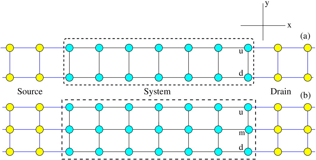
Figure 1: (Color online). Schematic view of (a) two-leg and (b) three-leg ladder networks (cyan colored sites) connected to semi-infinite multi-channel source and drain (yellow colored sites). The upper and the lower legs are marked ‘u’ and ‘d’ respectively for the two-leg ladder and ‘u’, ‘m’ and ‘d’ for the three-leg one.

method for this, and use a two-leg ladder as a prototype case for illustration. We prove that, this effect can be observed by tuning the relative phase difference of the lattice potential and the inter-arm hopping integrals. This is interesting as the ‘phases’ can now be controlled experimentally. The individual values of such phases do not not affect the bulk properties of a one-dimensional AAH model, preserving its self-duality, and yet, they are shown to exhibit nontrivial topological properties that are attributed to a higher dimensional system kraus . In addition, the quasiperiodic modulation in the hopping integrals in the commensurate limit turns out to be topologically nontrivial, supporting zero energy edge modes sankar1 .

It is pertinent to mention that, multi-leg ladders have become relevant recently after the experimental realization of double well optical lattices where bosonic atoms (⁸⁷Rb) are trapped sebby . A one-dimensional double well optical lattice is equivalent to a two legged ladder network danshita . Construction of such systems exploits the flexibility and control over the interfering laser beams, and trapping of bosonic or fermionic ultra-cold atoms leading to the realization of two and three legged ladders piraud ; greschner ; hugel ; kolley .

The result obtained here is in sharp contrast to a purely one-dimensional AAH model where the state transition occurs depending on the strength of the potential only, that is, in a parameter space rather than as a function of the Fermi energy, which is the case here. We present analytically exact results in details for a two-leg optical ladder lattice, and discuss the pathway to generalize this to multiple legs, leading finally to a two-dimensional structure.

The rest of the paper is arranged as follows. In the first part of Sec. II we present analytically exact results and in the second part of this section we give the theoretical prescription to simulate a real experimental situation by coupling the ladder to ideal semi-infinite leads. The numerical results are placed in Sec. III and finally we conclude in Sec. IV.

II Analytical argument and theoretical framework

Preservation of duality and spectral character in one-dimension

Before going into the actual problem addressed here, it is important to examine if the presence of a phase factor does, in any way, influence the spectral character of a one-dimensional AAH model. In its simplest form the on-site potential of an AAH model in a one-dimensional lattice of lattice constant $a$ is written as, $\epsilon_{n}=\lambda\cos(2\pi Qna+\varphi)$, where $Q$ is an irrational number, typically chosen as the golden mean $(\sqrt{5}+1)/2$ in what is called the incommensurate limit. $\lambda$ is the strength of the on-site potential and $\varphi$ is an arbitrary phase factor that shifts the origin of the potential. The Schrödinger equation, written in the form of a difference equation, relating the amplitudes $f_{n}$ on the neighboring sites on the lattice is given by,

$$[E-\lambda\cos(2\pi Qna+\varphi)]f_{n}=t(f_{n-1}+f_{n+1})$$ (1)

where, $t$ is the nearest-neighbor hopping integral. A discrete Fourier transform, $f_{n}=\exp(i\varphi na)\sum_{m}g_{m}\exp[im(2\pi Qna+\varphi)]$ maps Eq. 1 into

$$[E-t\cos(2\pi Qma+\varphi)]g_{m}=(\lambda/2)(g_{m-1}+g_{m+1})$$ (2)

The AAH model leads to the conclusion that, if $g_{m}$ is localized, that is, if $\sum_{m=-\infty}^{\infty}|g_{m}|^{2}$ is finite, then $f_{n}=\exp(i\varphi na)g_{m}\exp[im(2\pi Qna+\varphi)]$ represents an extended wave-function, i.e., $\sum_{n=-\infty}^{\infty}|f_{n}|^{2}$ diverges, and that, if $f_{n}$ is localized, then $g_{m}=\exp(i\varphi ma)\sum_{n}f_{n}\exp[in(2\pi Qma+\varphi)]$ will be extended in character. This is the essence of duality sokoloff . Eq. (2) thus tells us that the ‘duality’ is preserved even if we add an arbitrary phase to the potential.

With the assumed form of the on-site potential, viz, $\epsilon_{n}=\lambda\cos(2\pi Qna+\varphi)$, it now becomes a simple task to show that in the Fourier space the phase can be absorbed in the amplitude of the nearest neighbor hopping integral, making the effective on-site potential free of phase. The difference equation reads (in Fourier space),

$$\left[E-t\cos(2\pi Qma)\right]g_{m}=(\lambda/2)e^{-i\varphi}g_{m+1}+(\lambda/2)e^{i\varphi}g_{m-1}$$ (3)

It is obvious that, the effective hopping integrals in the Fourier space are $t^{eff}_{m,m\mp 1}\equiv(\lambda/2)\exp(\pm i\varphi)$. Since both the effective potential $\epsilon^{eff}_{m}\equiv t\cos(2\pi Qma)$ and the magnitude of the nearest-neighbor hopping integral $|t^{eff}_{m,m\pm 1}|$ do not depend on the phase $\varphi$, the density of states and the localization properties are in no way, affected by any variation of this phase. That is, we still retain the well known AAH conclusion that the single particle states will be extended, localized or critical if $\lambda$ is less than, greater than, or equal to $2t$ respectively.

In what follows we show that the situation is not so trivial in quasi one-dimensional cases, and with phases introduced in both the potential term and the hopping integrals along the rungs.

The case of a multi-leg ladder network: The metal-insulator transition

The model is schematically shown in Fig. 1, which mimics a two-leg optical lattice (a), and a three-leg one (b). The cyan colored sites represent the system of atoms loaded in the up (u) and down (d) legs. The rungs are along the $y$-direction. The leads needed for the transport calculation are shown by yellow dots. For a ladder extending to infinity along the $x$-direction, the Hamiltonian for the system (S), written in a tight-binding framework reads,

$$H_{S} = \sum_{n}\mbox{\boldmath$c_{n}^{\dagger}\epsilon_{n}c_{n}$}+\sum_{n}\left(\mbox{\boldmath$c_{n+1}^{\dagger}t$}\mbox{\boldmath$c_{n}$}+h.c.\right)$$ (4)

where, $n=-\infty...-1$, $0$, $1$, $2$, $\dots$, $\infty$ is the site index along the $x$-direction. The operators in Eq. 4 are as follows.
$c_{n}^{\dagger}$=$\left(\begin{array}[]{cc}c_{n,u}^{\dagger}&c_{n,d}^{\dagger}\end{array}\right);$ $c_{n}$=$\left(\begin{array}[]{c}c_{n,u}\\ c_{n,d}\end{array}\right);$ $\epsilon_{n}$=$\left(\begin{array}[]{cc}\epsilon_{n,u}&t_{n,y}\\ t_{n,y}&\epsilon_{n,d}\end{array}\right);$ $t$=$\left(\begin{array}[]{cc}t_{x}&0\\ 0&t_{x}\end{array}\right).$
Here $\epsilon_{n,u(d)}$ is the on-site potential at the $n$-th site of the ‘up’ (u) or ‘down’ (d) leg. We choose $\epsilon_{n,u}=\epsilon_{n,d}=\lambda\cos(2\pi Qn+\varphi_{\nu})=\epsilon_{n}$ (say). The lattice constant $a$ is chosen as unity. $t_{n,y}$ is quasiperiodically modulated hopping integral along the $n$-th rung and is chosen as, $t_{n,y}=t_{y}\cos(2\pi Qn+\varphi_{\beta})$. $Q$ will be chosen as the golden ratio $(\sqrt{5}+1)/2$, whose rational approximants have been exploited to explore the topological states in the 1D version of the lattice sankar1 . $c_{n,u(d)}^{\dagger}$ ($c_{n,u(d)}$) is the creation (annihilation) operator of a particle at the $n$-th site in the up or down arm of the ladder. We have kept the hopping integral along the $x$-direction constant, and equal to $t_{x}$. A variation in $t_{x}$ can easily be dealt with in the present formalism.

Let us explain the scheme by analyzing the spectrum of a two legged ladder of infinite extension along the $x$-direction. The Schrödinger equation for such a ladder network can equivalently be written down in the form of a couple of difference equations, viz.,

$$(E-\epsilon_{n,u})\psi_{n,u} = t_{x}(\psi_{n+1,u}+\psi_{n-1,u})+t_{n,y}\psi_{n,d}$$

$$(E-\epsilon_{n,d})\psi_{n,d} = t_{x}(\psi_{n+1,d}+\psi_{n-1,d})+t_{n,y}\psi_{n,u}$$ (5)

We have chosen to set, for our purpose, $\epsilon_{n,u}=\epsilon_{n,d}=\epsilon_{n}$. In that case, it is easily seen that, the potential and the hopping matrices are nothing but, $\mbox{\boldmath$\epsilon_{n}$}=\epsilon_{n}\mbox{\boldmath$I$}+t_{n,y}\mbox{\boldmath$\sigma_{x}$}$, and $\mbox{\boldmath$t$}=t_{x}\mbox{\boldmath$I$}$, where, $\sigma_{x}$ and $I$ are the Pauli matrix and the $2\times 2$ identity matrix respectively. It now becomes obvious that, the commutator $[\mbox{\boldmath$\epsilon_{n}$},\mbox{\boldmath$t$}]=0$ independent of the rung index ‘$n$’. This allows us to diagonalize the potential and the hopping matrices simultaneously and make a uniform change of basis, going from the Wannier orbitals $\mbox{\boldmath$\Psi_{n}$}\equiv(\psi_{n,u},\psi_{n,d})$ to $\mbox{\boldmath$\Phi_{n}$}\equiv(\phi_{n,u},\phi_{n,d})=\mbox{\boldmath$M^{-1}$}\mbox{\boldmath$\Psi_{n}$}$.

The change of basis decouples the set of Eq. (5) as,

$$\left[E-\lambda_{1}\cos(2\pi Qn+\xi_{1})\right]\phi_{n,u} = t_{x}(\phi_{n+1,u}+\phi_{n-1,u})$$

$$\left[E-\lambda_{2}\cos(2\pi Qn+\xi_{2})\right]\phi_{n,d} = t_{x}(\phi_{n+1,d}+\phi_{n-1,d})$$

where,
$\lambda_{1}=\sqrt{\lambda^{2}+t_{y}^{2}+2\lambda t_{y}\cos(\phi_{\nu}-\phi_{\beta})},\\ \lambda_{2}=\sqrt{\lambda^{2}+t_{y}^{2}-2\lambda t_{y}\cos(\phi_{\nu}-\phi_{\beta})},\\ \xi_{1}=\tan^{-1}[(\lambda\sin\phi_{\nu}+t_{y}\sin\phi_{\beta})/(\lambda\cos\phi_{\nu}+t_{y}\cos\phi_{\beta})],\\ \xi_{2}=\tan^{-1}[(\lambda\sin\phi_{\nu}-t_{y}\sin\phi_{\beta})/(\lambda\cos\phi_{\nu}-t_{y}\cos\phi_{\beta})]$.
The new states are,

$$\phi_{n,u} = (-1/2)\psi_{n,u}+(1/2)\psi_{n,d}$$

$$\phi_{n,d} = (1/2)\psi_{n,u}+(1/2)\psi_{n,d}$$ (7)

and it should be appreciated that $\phi_{n,u(d)}$ can be localized only when both $\psi_{n,u(d)}$ are localized. If any of the original Wannier orbital $\psi_{n,u(d)}$ corresponds to an extended eigenstate, then the new state $\phi_{n,u}$ will retain its extended character.

It is apparent that, the first (or the second) of the set of Eq. (LABEL:decouple) will give extended, localized or critical eigenstates for $\lambda_{1}$ (or $\lambda_{2}$) $<$, $>$ or $=2t_{x}$  aubry . This implies that, if we set for example, $\lambda_{1}<2t_{x}$, the first of the Eq. (LABEL:decouple) will yield an absolutely continuous spectrum, while the second one can give rise to a pure point, critical or even absolutely continuous energy spectrum depending on the magnitude of $\lambda_{2}$ with the choice of parameters prefixed for $\lambda_{1}$. Thus we have an option of engineering the spectrum. As the density of states of the full quasi-one dimensional ladder will come from a convolution of the two densities of states obtained from the two decoupled equations, we have the provision of engineering the full density of states, creating even a mixed one with localized and extended eigenfunctions. The possibility of a re-entrant metal to insulator crossover is thus on the cards.

In Fig. 2 we have shown the contour plot of the strength of the on-site potential $\lambda_{1}$ as the relative phase difference $\Delta\varphi=\varphi_{\nu}-\varphi_{\beta}$ is varied against a wide choice of the basic potential strength $\lambda$. We have set the amplitude of the transverse hopping $t_{y}=1$. The contours correspond to various values of $\lambda_{1}$ less than, or greater than $2t_{x}=2$ (with $t_{x}$ being set equal to unity) depending on the combination $(\lambda$, $\Delta\varphi)$. The observation is similar for $\lambda_{2}$ as well. If one dwells in that regime of the parameter subspace $(\lambda_{1(2)}$, $\Delta\varphi)$, where $\lambda_{1}$ is less than $2t_{x}$, (red dotted contours) while $\lambda_{2}$ can be tuned (by $\Delta\varphi$) to be greater than $2t_{x}$, then the first of the decoupled equations Eq. (LABEL:decouple) yields an absolutely continuous spectrum, while the second one gives rise to a pure point spectrum. The energy spectrum of the two arm ladder network is a mixed one then, as discussed before, comprising an absolutely continuous part populated by Bloch like extended states and exponentially localized states

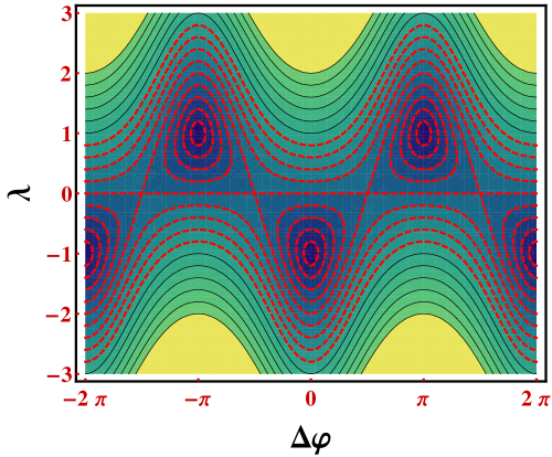
Figure 2: (Color online). Variation of the strength of the effective potential $\lambda_{1}$ as a function of the original strength of potential $\lambda$ and the relative phase difference $\Delta\varphi=\phi_{\nu}-\phi_{\beta}$. We have set $t_{x}=1$ and $t_{y}=1$. The red dotted contours provide combinations of $(\Delta\varphi,\lambda)$ for which the values of $\lambda_{1}$ is less than $2$.

arising out of the second of the Eq. (LABEL:decouple). The proximity of the edges of the extended band and the subclusters formed by the localized eigenfunctions will determine the possibility of a metal-insulator transition. This is sensitive to the appropriate choice of the phase difference $\Delta\varphi$ and $\lambda$.

To check the truthfulness of the above analysis, we consider non-interacting, spinless electrons on a two legged ladder network. For this system, we evaluate the density of states and multi-channel transport with an AAH variation in both the potentials $\epsilon_{n}$ and the inter-arm hopping integral $t_{y}$, as given in the previous discussion and including the phases. To simulate a real experimental situation we clamp an $N$-rung two-legged ladder at its extremities to ideal semi-infinite ‘electrodes’ (leads) of finite width, and evaluate the average density of states of a finite sized system with the leads attached. The Hamiltonian of the electrodes is taken to be $H_{0}$ $+$ $H_{LS}$ $+$ $H_{RS}$ where,

$$H_{0} = \sum_{n=-\infty}^{0}\mbox{\boldmath$c_{n}^{\dagger}\epsilon_{0}c_{n}$}+\sum_{n=N+1}^{\infty}\mbox{\boldmath$c_{n}^{\dagger}\epsilon_{0}c_{n}$}$$ (8)

$$+\sum_{n}\left(\mbox{\boldmath$c_{n+1}^{\dagger}t_{0}$}\mbox{\boldmath$c_{n}$}+h.c.\right)$$

with, $\epsilon_{0}$=$\left(\begin{array}[]{cc}\epsilon_{0}&\tau_{y}\\ \tau_{y}&\epsilon_{0}\end{array}\right)$ and $t_{0}$=$\left(\begin{array}[]{cc}\tau_{x}&0\\ 0&\tau_{x}\end{array}\right).$
$\tau_{x}$ and $\tau_{y}$ are the hopping integrals in the leads, along the $x$ and the $y$-directions respectively. The couplings between the left (L) and the right (R) electrodes, and the system (S) are given by, $\mbox{\boldmath$H_{LS}$}=\mbox{\boldmath$c_{0}^{\dagger}$}\mbox{\boldmath$t_{L}$}\mbox{\boldmath$c_{1}^{\dagger}$}$, and $\mbox{\boldmath$H_{RS}$}=\mbox{\boldmath$c_{N}^{\dagger}$}\mbox{\boldmath$t_{R}$}\mbox{\boldmath$c_{N+1}^{\dagger}$}$ respectively, with, $t_{L}(R)$=$\left(\begin{array}[]{cc}\tau_{L(R)S}&0\\ 0&\tau_{L(R)S}\end{array}\right)$. The average density of states of the electrode-system-electrode network is given, in Green’s function formalism as,

$$\rho_{av}=-\frac{1}{N\pi}\mbox{Im}[\mbox{Tr}\,\mbox{\boldmath$G$}]$$ (9)

where, $\mbox{\boldmath$G$}=[(E+i\eta)\mbox{\boldmath$I$}-\mbox{\boldmath$H$}]^{-1}$, The full Hamiltonian $\mbox{\boldmath$H$}=\mbox{\boldmath$H_{LS}$}+\mbox{\boldmath$H_{S}$}+\mbox{\boldmath$H_{RS}$}$. In terms of the Green’s function of the system and the electrode-system couplings, the transmission coefficient across the system is written as datta

$$T=\mbox{Tr}[\mbox{\boldmath$\Gamma_{L}$}\mbox{\boldmath$G_{S}^{r}$}\mbox{\boldmath$\Gamma_{R}$}\mbox{\boldmath$G_{S}^{a}$}]$$ (10)

Here, $G_{S}^{r}$ and $G_{S}^{a}$ are the ‘retarded’ and the ‘advanced’ Green’s functions respectively, of the two leg ladder network, including the effects of the leads. The Green’s function for the system concerned is expressed as,

$$\mbox{\boldmath$G_{S}$}=(E\mbox{\boldmath$I$}-\mbox{\boldmath$H_{S}$}-\mbox{\boldmath$\Sigma_{L}$}-\mbox{\boldmath$\Sigma_{R}$})^{-1}$$ (11)

where, $\Sigma_{L(R)}$ are the self energies and take care of the system-electrode coupling datta .

III Numerical results

In Fig. 3 and Fig. 4 we show the density of states (panel (a)) and the transmission coefficient (panel (b)) for a $40$-rung ladder network with $\varphi_{\nu}=\varphi_{\beta}=0$, and $\varphi_{\nu}=0$, $\varphi_{\beta}=\pi/2$ respectively. We have set $\lambda=1.5$, $t_{y}=1$, $Q=(\sqrt{5}+1)/2$ and $t_{x}=1$. The imaginary part added to the energy, viz. $\eta$ has been taken to be $2\times 10^{-9}$, and the chemical potential has been set equal to zero. With the above choice of parameters, and when $\phi_{\nu}=\phi_{\beta}=0$, we find $\lambda_{1}=2.5$ which is greater than $2t_{x}=2$, and hence the first set of equations Eq. (LABEL:decouple) yields a localized spectrum. However, $\lambda_{2}=0.5$ in this case, and is less than $2t_{x}=2$, and the second of the set of Eq. (LABEL:decouple) yield an absolutely continuous spectrum populated by extended states only. In Fig. 3 we thus observe a mixed spectrum, the extended zone $-2<E<2$ destroying the localized character of the eigenstates arising out of the second equation. The localized states which lie outside this ‘extended state zone’ appear as spikes, densely packed towards the flanks. The transmission coefficient corresponding to the extended eigenstates residing in the absolutely continuous parts of the spectrum turns out to be high and corroborates the conclusion about the character of the eigenfunctions.

In contrary to this, in Fig. 4, both $\lambda_{1}$ and $\lambda_{2}$ turn out to be equal to $\sqrt{3.25}$ which is less that $2t_{x}=2$. Only extended states are generated by each of the decouple equations in Eq. (LABEL:decouple). Thus the full spectrum

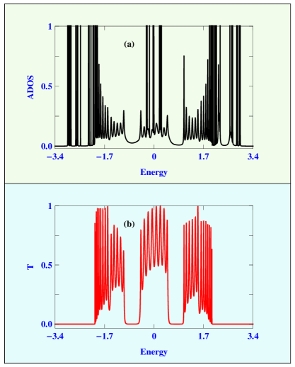
Figure 3: (Color online). (a) Density of states and (b) the transmission characteristics of the two arm aperiodic ladder network with $40$ rungs. Here, $\varphi_{\nu}=\varphi_{\beta}=0$, $\lambda=1.5$, $t_{x}=t_{y}=1$, $\tau_{x}=\tau_{y}=2$, $t_{L(R)}=1$ and $Q=(\sqrt{5}+1)/2$. The chemical potential is set at zero.

of the two-leg ladder consists of extended eigenstates only. This is precisely corroborated by the transmission characteristics shown in Fig. 4, which show clusters of finite transmission exactly at the place where the density of states turns out to be non-zero. The system now, is totally metallic. Thus, just by tuning the relative phases one can engineer whether to have a metallic system out of the ladder network or to create a mixed spectrum for the same where one can see a non-metallic (insulating) and metallic (conducting) character depending on the position of the Fermi level.

Getting back to the discussion of Fig. 3,the prime interest lies in the regions in between the subclusters of extended states around $E=\pm 0.85$ where the density of states in low, but finite and remains finite even if we lower the value of the imaginary part $\eta$ further. We have scanned this region by decreasing the energy interval gradually. The states occupying this zone in the energy scale appear as sharp peak (the peak structure is not visible at this scale) and form a dense cluster that appears almost as continuous. This is concluded from finer and finer scanning of the energy interval around $E=\pm 0.85$. The corresponding transmission for all such states is zero. This signifies that these are sub-bands of exponentially localized eigenstates.

On close scrutiny, done numerically, it also appears that such minibands of localized eigenstates merge with the neighboring absolutely continuous bands of extended states in a continuous manner i.e., we were unable to detect any clear separation between the end of the band of localized states and the beginning of the band of extended

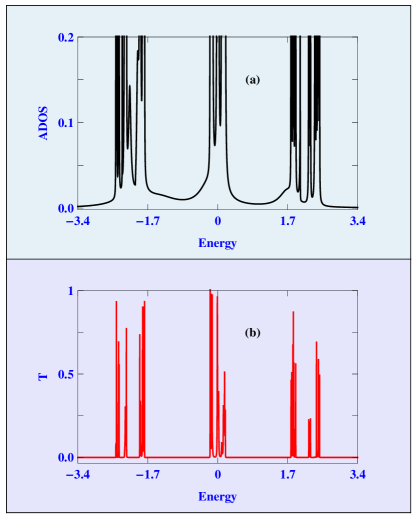
Figure 4: (Color online). (a) Density of states and (b) the transmission characteristics of the two arm aperiodic ladder network with $40$ rungs when $\phi_{\nu}=0$ and $\phi_{\beta}=\pi/2$. We take $\lambda_{1}=\lambda_{2}=\sqrt{3.25}$, and the values of other parameters are same as taken in Fig. 3.

eigenstates. This happens also, in the same manner, as one crosses the band of high transmission and re-enter into the next miniband of localized states. This tempts us to conclude that a re-entrant metal-insulator transition is definitely a possibility here, as anticipated from the exact analytical treatment presented before. The same kind of behavior is observed when we have chosen $\Delta\varphi=\pi/2$, as shown in Fig. 4. Here, $\lambda_{1}=\lambda_{2}=\sqrt{3.25}$ and less than $2t_{x}$. The non-zero DOS regimes and their corresponding zero transmission values strengthen our surmise that, a re-entrant metal-insulator transition can indeed be triggered by a variation of the phase difference $\Delta\varphi=\varphi_{\nu}-\varphi_{\beta}$.

It would be interesting to link such observations to experiments with Bose-Einstein condensates released into one-dimensional waveguides in the presence of a controlled disorder roati ; billy . A typical method to extract information about localization has been to photograph the atomic density profiles roati ; billy as a function of time. Disorder is found to stop the expansion of the wave packet and lead to the formation of exponentially localized wave function roati ; billy . In a very recent experiment Schreiber et al. schreiber made a direct observation of quantum many body localization in interacting fermionic systems using ${}^{40}K$ atoms in a trap of an AAH potential profile with a phase offset. They have measured the ‘imbalance’ $I=(N_{e}-N_{o})/(N_{e}+N_{o})$ between the occupation of the ‘odd’ (o) and ‘even’ (e) sites in the optical lattice. $I$ essentially measures the charge density wave (CDW) order which basically acts as an order parameter to characterize localization effects, and incidentally any possible localization-de localization transition. For strong localization, the particles remain localized to the initial locations they were ‘released’ into. The CDW is smeared a little bit. For extended eigenstates, the localization length increases and the steady state value of the CDW is lowered schreiber . A weak atomic density can result in a negligible interaction among the particles and the non-interacting limit can be achieved. The theory presented in this communication can thus be taken as a proposal for verifying the existence of a metal-insulator like behavior

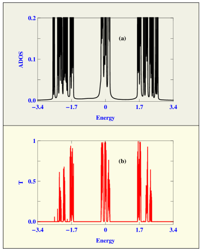
Figure 5: (Color online). (a) Density of states and (b) the transmission coefficient of a three arm ladder network with leads of the same width attached to it. There are $100$ rungs, and we have chosen $\phi_{\nu}=0$, $\phi_{\beta}=\pi/2$, $\lambda=1.5$, $t_{x}=t_{y}=1$, $\tau_{x}=\tau_{y}=2$ and $t_{L(R)}=1$.

in quasi one-dimension and in the non-interacting limit, in the spirit of the above experiments. The likely changes in the relaxation dynamics of the CDW as mentioned above can bring out the role played by the phase difference in regard of the metal-insulator transition.

Extending the above idea to multi-leg ladder networks is trivial. For an $N$-leg ladder, the difference equations can be split into a set of $N$ decoupled equations. Depending on the relative phase difference, any one or more of them can render absolutely continuous spectrum and/or a mixing of the same with pure point spectrum, leading to the possibility of a metal-insulator transition in quasi one- or even two-dimensional quasiperiodic optical lattice models. We test it out with a three-leg ladder with $100$ rungs. The results are shown in Fig. 5 and, are self explanatory, in the light of the discussions for the two-leg case.

IV Conclusion

In conclusion, we have shown analytically that an infinite multi-leg optical lattice with quasiperiodic modulation in the potential profile and in the inter-arm hopping integral can exhibit multiple mobility edges if one engineers the phase difference of the modulation profiles appropriately by tuning the coherence of the trapping laser beams. Exact results corroborated by numerical analysis are discussed specifically for a double legged ladder which can be thought to mimic asymmetric double well potentials and ultra-cold atoms trapped in higher orbital bands in an optical lattice. The results can stimulate experiments to verify the very fundamental issues like Anderson localization, metal-insulator transitions etc, and may turn out to be useful in designing nano devices.

V Acknowledgments

A.C. thanks a DST-PURSE grant through the University of Kalyani, and Atanu Nandy for one of the graphics.

References

- (1) D. Jaksch and P. Zoller, Ann. Phys. 315, 52 (2005).
- (2) I. Bloch, J. Dalibard, and W. Zwerger, Rev. Mod. Phys. 80, 885 (2008).
- (3) M. Lewenstein, A. Sanpera, and V. Ahufinger, Ultracols atoms in optical lattices: simulating Quantum Many-Body systems, Oxford University Press, UK (2012).
- (4) O. Dutta et al., Rep. Prog. Phys. 78, 066001 (2015).
- (5) O. Dutta, A. Przysiezna, and J. Zakrzewski, Sci. Rep. 5, 11060 (2015).
- (6) M. Greiner et al., Nature 415, 39 (2002).
- (7) M. Aidelsburger et al., Phys. Rev. Lett. 111, 185301 (2013).
- (8) H. Miyake, G. Siviloglou, C. J. Kennedy, W. C. Burton, and W. Ketterle, Phys. Rev. Lett. 111, 185302 (2013).
- (9) G. Sun, Phys. Rev. A 93, 023608 (2016).
- (10) S. Aubry and G. André, Ann. Isr. Phys. Soc. 3, 133 (1980).
- (11) L. Dal Negro et al., Phys. Rev. Lett. 90, 055501 (2003).
- (12) Y. Lahini et al., Phys. Rev. Lett. 103, 013901 (2009).
- (13) Y. E. Kraus et al., Phys. Rev. Lett. 109, 106402 (2012).
- (14) G. Roati et al., Nature 453, 895 (2008).
- (15) S. Ganeshan, K. Sun, and S. Das Sarma, Phys. Rev. Lett. 110, 180403 (2013).
- (16) G. Modugno, Rep. Prog. Phys. 73, 102401 (2010).
- (17) P. W. Anderson, Phys. Rev. 109, 1492 (1958).
- (18) J. Sebby-Strabley, M. Anderlini, P. S. Jessen, and J. V. Porto, Phys. Rev. A 73, 033605 (2006).
- (19) I. Danshita, J. E. Williams, C. A. R. Sá de Melo, and C. W. Clark, Phys. Rev. A 76, 043606 (2007).
- (20) M. Piraud et al., Phys. Rev. B 91, 140406 (2015).
- (21) S. Greschner et al., Phys. Rev. Lett. 115, 190402 (2015).
- (22) D. Hügel and B. Paredes, Phys. Rev. A 89, 023619 (2014).
- (23) F. Kolley et al., New J. Phys. 17, 092001 (2015).
- (24) J. B. Sokoloff, Phys. Rep. 126, 189 (1985).
- (25) S. Datta, Electronic transport in mesoscopic systems, Cambridge University Press, Cambridge (1997).
- (26) J. Billy et al., Nature 453, 891 (2008).
- (27) M. Schreiber et al., Science 349, 842 (2015).