Prescribing the mixed scalar curvature
of a foliated Riemann-Cartan manifold

Abstract

The mixed scalar curvature is one of the simplest curvature invariants of a foliated Riemannian manifold. We explore the problem of prescribing the mixed scalar curvature of a foliated Riemann-Cartan manifold by conformal change of the structure in tangent and normal to the leaves directions. Under certain geometrical assumptions and in two special cases: along a compact leaf and for a closed fibred manifold, we reduce the problem to solution of a leafwise elliptic equation, which has three stable solutions – only one of them corresponds to the case of a foliated Riemannian manifold.

Keywords: foliation, pseudo-Riemanian metric, contorsion tensor, mixed scalar curvature, conformal, leafwise Schrödinger operator, elliptic equation, attractor

Mathematics Subject Classifications (2010) Primary 53C12; Secondary 53C44

Introduction

Geometrical problems of prescribing curvature invariants of Riemannian manifolds using conformal change of metric are popular for a long time, i.e., the study of constancy of the scalar curvature was began by Yamabe in 1960 and completed by Trudinger, Aubin and Schoen in 1986, see [2].

The metrically-affine geometry was founded by E. Cartan in 1923–1925, who suggested using an asymmetric connection $\bar{\nabla}$ instead of Levi-Civita connection $\nabla$ of $g$; in extended theory of gravity the torsion of $\bar{\nabla}$ is represented by the spin tensor of matter. Notice that $\bar{\nabla}$ and $\nabla$ are projectively equivalent (have the same geodesics) if and only if the difference $\mathfrak{T}:=\bar{\nabla}-\nabla$, called the contorsion tensor, is antisymmetric. Riemann-Cartan (RC) spaces, i.e., with metric connection: $\bar{\nabla}g=0$, appear in such topics as homogeneous and almost Hermitian spaces [5], and geometric flows [1].

Foliations, i.e., partitions of a manifold into collection of submanifolds, called leaves, arise in topology and have applications in differential geometry, analysis and theoretical physics, where many models are foliated. One of the simplest curvature invariants of a foliated Riemannian manifold is the mixed scalar curvature ${\rm S}_{\rm mix}$, i.e., an averaged sectional curvature over all planes that contain vectors from both – tangent and normal – distributions, see [9]. The prescribing of ${\rm S}_{\rm mix}$ by conformal change of the metric in normal to the leaves directions and certain Yamabe type problem have been studied in [12, 13]. In the paper, we examine the problem of prescribing the mixed scalar curvature $\bar{\rm S}_{\,\rm mix}$ of a foliated RC manifold by conformal change of the structure in tangent and normal to the leaves directions. In particular, we explore the following Yamabe type problem:

Given foliated RC manifold $(M,g,\bar{\nabla})$ find a $({\cal D},{\cal D}^{\perp})$-conformal RC structure, i.e.,

$$g^{\prime}=g^{\top}+u^{2}\,g^{\bot},\qquad{\mathfrak{T}^{\prime}}=u^{2}\,\mathfrak{T}^{\top}+\mathfrak{T}^{\bot},$$ (1)

with (leafwise) constant mixed scalar curvature. Here $u\in C^{\infty}(M)$ is positive and

$$g^{\top}(X,Y):=g(X^{\top},Y^{\top}),\quad g^{\perp}(X,Y):=g(X^{\perp},Y^{\perp}),\quad\mathfrak{T}^{\top}_{X}Y:=(\mathfrak{T}_{X}Y)^{\top},\quad\mathfrak{T}^{\bot}_{X}Y:=(\mathfrak{T}_{X}Y)^{\bot}.$$

We show that under certain geometric assumptions, including $\nabla$-harmonicy of ${\cal F}$ and $g_{\,|\,T{\cal F}}>0$, the conformal factor in (1) obeys leafwise elliptic equation

$$-\Delta^{\top}u-\beta(x)\,u=\Psi_{1}(x)\,u^{-1}-\Psi_{2}(x)\,u^{-3}+\Psi_{3}(x)\,u^{3}$$ (2)

with smooth functions $\beta$ and $\Psi_{i}\ (i=1,2,3)$ described in Section 1.2. The case of $g_{\,|T{\cal F}}<0$ reduces to the above by change $g\rightarrowtail-g$. Notice that $\Psi_{3}$ represents the novel mixed scalar $\mathfrak{T}^{\top}$-curvature, see Section 1.1, and the stable solution of (2) in the case of $\Psi_{3}=0$ has been found in [13]. By stable solution of elliptic equation we mean a stable stationary solution of its parabolic counterpart.

Using spectral parameters of the Schrödinger operator along compact leaves,

$$\mathcal{H}:u\mapsto-\Delta^{\top}u-\beta(x)\,u,$$ (3)

we prove that (2) has three stable solutions, one of them ($\Psi_{3}=0$) corresponds to the Riemannian case.

Since the topology of the leaf through a point can change dramatically with the point, there are difficulties in studying leafwise elliptic equations. Thus, we examine two formulations of the problem:

1. $\bar{\rm S}_{\,\rm mix}$ is prescribed on a compact leaf $F$. Under some geometric assumptions we get (2), whose solutions $u_{*}{\in}C^{\infty}(F)$ form a compact set in $C(F)$ and can be extended smoothly onto $M$.

2. $\bar{\rm S}_{\,\rm mix}$ is prescribed on a closed manifold $M$. Under certain geometric assumptions we get (2) on any $F$, whose unique solution $u_{*}\in C^{\infty}(F)$ on any leaf $F$ belongs to $C^{\infty}(M)$ when

$${{\cal F}}\ \ \textrm{is defined by an orientable fiber bundle}\ \ {\pi:M\to B.}$$ (4)

The main results of the paper are Theorems 1– 3 (and their corollaries) about foliations of arbitrary (co)dimension, similar results for codimension-one foliations and flows are omitted.

The paper is organized as follows. Section 1 contains geometrical results of our paper. Section 1.1 gives preliminaries for foliated RC manifolds. Section 1.2 derives the transformation law for $\bar{\rm S}_{\,\rm mix}$ under $({\cal D},{\cal D}^{\bot})$-conformal change of RC structure; this yields, under certain geometrical assumptions, elliptic equation (2) for the conformal factor. The results in Section 1.3 are separated into three cases according the sign of the mixed scalar $\mathfrak{T}^{\top}$-curvature represented by $\Psi_{3}$. To prescribe $\bar{\rm S}_{\,\rm mix}$ on a closed leaf (Theorem 1) we use the existence of a solution to (2), and to prescribe $\bar{\rm S}_{\,\rm mix}$ on a closed fibred manifold (Theorem 2) we use the existence and uniqueness of a solution to (2), see Section 2, where we also prove that (2) has three stable solutions, which are expressed in terms of spectral parameters of operator (3).

1 Foliated Riemann-Cartan manifolds

1.1 The mixed scalar curvature

A pseudo-Riemannian metric of index $q$ on manifold $M$ is an element $g\in{\rm Sym}^{2}(M)$ (of the space of symmetric $(0,2)$-tensor fields) such that each $g_{x}\ (x\in M)$ is a non-degenerate bilinear form of index $q$ on the tangent space $T_{x}M$. When $q=0$, $g$ is a Riemannian metric (resp. a Lorentz metric when $q=1$). Let $\mathfrak{X}_{M}$ be the module over $C^{\infty}(M)$ of all vector fields on $M$.

The Levi-Civita connection $\nabla:\mathfrak{X}_{M}\times\mathfrak{X}_{M}\to\mathfrak{X}_{M}$ of $g$, represented using the Lie bracket,

$$\quad 2\,g(\nabla_{X}\,Y,Z)=Xg(Y,Z)+Yg(X,Z)-Z\,g(X,Y)$$

$$+\,g([X,Y],Z)-g([X,Z],Y)-g([Y,Z],X)\quad(X,Y,Z\in\mathfrak{X}_{M}),$$ (5)

is metric compatible, $\nabla g=0$, and has zero torsion.

A subbundle ${\cal D}\subset TM$ (called a distribution) is non-degenerate, if ${\cal D}_{x}$ is a non-degenerate subspace of $(T_{x}M,\,g_{x})$ for $x\in M$; in this case, its orthogonal distribution ${\cal D}^{\bot}\subset TM$ is also non-degenerate. Thus, we consider a connected manifold $M^{n+p}$ with a pseudo-Riemannian metric $g$ and complementary orthogonal non-degenerate distributions ${\cal D}$ and ${\cal D}^{\bot}$ of ranks $\dim_{\,\mathbb{R}}{\cal D}_{x}=p\geq 1$ and $\dim_{\,\mathbb{R}}{\cal D}^{\bot}_{x}=n\geq 1$ for every $x\in M$ (called an almost-product structure on $M$), see [3].

Let $X^{\top}$ be the ${\cal D}$-component of $X\in\mathfrak{X}_{M}$ (resp., $X^{\perp}$ the ${\cal D}^{\bot}$-component of $X$), and $\mathfrak{X}^{\top}_{M}$ (resp. $\mathfrak{X}^{\bot}_{M}$) the module over $C^{\infty}(M)$ of all vector fields in ${\cal D}$ (resp. ${\cal D}^{\bot}$). In the paper, ${\cal D}$ is integrable and tangent to a foliation ${\cal F}$. The integrability tensor of ${\cal D}^{\bot}$ is defined by $T^{\bot}(X,Y)=\frac{1}{2}\,[X,\,Y]^{\top}\ (X,Y\in\mathfrak{X}^{\bot}_{M})$, the second fundamental forms of ${\cal D}$ and ${\cal D}^{\bot}$ are given by

$$h^{\top}(X,Y)=(\nabla_{X}Y)^{\bot}\ \ (X,Y\in\mathfrak{X}^{\top}_{M}),\quad h^{\bot}(X,Y)=(\nabla_{X}Y+\nabla_{Y}X)^{\top}/2\ \ (X,Y\in\mathfrak{X}^{\bot}_{M}),$$

and mean curvature vectors are $H^{\top}=\operatorname{Tr}_{g}h^{\top}$ and $H^{\bot}=\operatorname{Tr}_{g}h^{\bot}$. We call ${\cal D}$ totally umbilical, harmonic, or totally geodesic, if $h^{\top}=\frac{1}{p}\,H^{\top}g^{\top},\ H^{\top}=0$, or $h^{\top}=0$, resp. Examples of harmonic foliations are parallel circles or winding lines on a flat torus and a Hopf field of great circles on $S^{3}$.

Recall that a linear connection $\bar{\nabla}$ on $M$ is a map $\bar{\nabla}:\mathfrak{X}_{M}\times\mathfrak{X}_{M}\to\mathfrak{X}_{M}$ with the properties:

$$\bar{\nabla}_{fX_{1}+X_{2}}Y=f\bar{\nabla}_{X_{1}}Y+\bar{\nabla}_{X_{2}}Y,\quad\bar{\nabla}_{X}(fY+Z)=X(f)Y+f\bar{\nabla}_{X}Y+\bar{\nabla}_{X}Z,$$

where $f\in C^{\infty}(M)$. Thus, linear connections over $M$ form an affine space, and the difference of two connections is a $(1,2)$-tensor.

Computing terms in the definition $\bar{R}_{X,Y}=[\bar{\nabla}_{Y},\bar{\nabla}_{X}]+\bar{\nabla}_{[X,Y]}$ of the curvature tensor of $\bar{\nabla}=\nabla+\mathfrak{T}$, and comparing with similar formula for $R_{X,Y}$, we find the following relation:

$$\bar{R}_{X,Y}=R_{X,Y}+(\nabla_{Y}\mathfrak{T})_{X}-(\nabla_{X}\mathfrak{T})_{Y}+[\mathfrak{T}_{Y},\mathfrak{T}_{X}].$$ (6)

Let $\{E_{a},\,{\cal E}_{i}\}_{a\leq p,\,i\leq n}$ be a local orthonormal frame on $TM$ such that $\{E_{a}\}\subset{\cal D}$ and $\{{\cal E}_{i}\}\subset{\cal D}^{\bot}$ and $\epsilon_{a}=g(E_{a},E_{a}),\ \epsilon_{i}=g({\cal E}_{i},{\cal E}_{i})$. We use the following convention for various tensors: $\mathfrak{T}_{i}=\mathfrak{T}_{{\cal E}_{i}}$ etc. The following function on a metric-affine manifold $(M,g,\bar{\nabla})$:

$$\bar{\rm S}_{\rm mix}=\frac{1}{2}\sum\nolimits_{a,i}\epsilon_{a}\epsilon_{i}\big{(}g({\bar{R}}_{E_{a},{\cal E}_{i}}E_{a},{\cal E}_{i})+g({\bar{R}}_{{\cal E}_{i},E_{a}}{\cal E}_{i},E_{a})\big{)}$$ (7)

is well-defined and is called the mixed scalar curvature of $(\widetilde{\cal D},{\cal D})$. This definition does not depend on the order of distributions and on the choice of a local frame. Moreover, see (6),

$$\hskip-25.60747pt\bar{\rm S}_{\rm mix}={\rm S}_{\rm mix}+Q,\ \ {\rm where}$$

$$\hskip-25.60747ptQ=\frac{1}{2}\sum\nolimits_{a,i}\epsilon_{a}\epsilon_{i}\big{(}g((\nabla_{i}\mathfrak{T})_{a}E_{a},{\cal E}_{i})-g((\nabla_{a}\mathfrak{T})_{i}E_{a},{\cal E}_{i})+g([\mathfrak{T}_{i},\,\mathfrak{T}_{a}]E_{a},{\cal E}_{i})$$

$$+\,g((\nabla_{a}\mathfrak{T})_{i}{\cal E}_{i},E_{a})-g((\nabla_{i}\mathfrak{T})_{a}{\cal E}_{i},E_{a})+g([\mathfrak{T}_{a},\,\mathfrak{T}_{i}]\,{\cal E}_{i},E_{a})\big{)}\,,$$ (8)

and ${\rm S}_{\rm mix}$ is the mixed scalar curvature of $\nabla$, see [9, 16]. Recall the formula:

$${\rm S}_{\,\rm mix}=g(H^{\bot},H^{\bot})-\langle h^{\bot},h^{\bot}\rangle+\langle T^{\bot},T^{\bot}\rangle+g(H^{\top},H^{\top})-\langle h^{\top},h^{\top}\rangle+\operatorname{div}(H^{\bot}+H^{\top}).$$ (9)

For a vector field on $M$ and for the gradient and Laplacian of a function $f\in C^{\infty}(M)$ we have

$$\hskip-17.07164pt\operatorname{div}X=\operatorname{div}^{\bot}X+\operatorname{div}^{\top}X,\quad\operatorname{div}^{\bot}X=\sum\nolimits_{\,i}\epsilon_{i}\,g(\nabla_{{\cal E}_{i}}X,\,{\cal E}_{i}),\quad\operatorname{div}^{\top}X=\sum\nolimits_{\,a}\epsilon_{a}\,g(\nabla_{E_{a}}X,\,E_{a}),$$

$$\hskip-17.07164ptg(\nabla f,X)=X(f),\qquad\Delta\,f=\operatorname{div}(\,\nabla f).$$

We also use notations for traces of $\mathfrak{T}$: $\operatorname{Tr}^{\bot}\mathfrak{T}:=\sum\nolimits_{\,i}\epsilon_{i}\,\mathfrak{T}_{i}\,{\cal E}_{i}$ and $\operatorname{Tr}^{\top}\mathfrak{T}:=\sum\nolimits_{\,a}\epsilon_{a}\,\mathfrak{T}_{a}E_{a}$.

Among all metric-affine spaces $(M,g,\bar{\nabla})$, RC spaces have metric compatible connection, i.e.,

$$g(\mathfrak{T}_{X}Y,Z)=-g(\mathfrak{T}_{X}Z,Y)\quad(X,Y,Z\in\mathfrak{X}_{M}).$$ (10)

The leaves of a foliation ${\cal F}$ on $(M,g,\bar{\nabla})$ are submanifolds with induced metric $g^{\top}$ and metric connection $\bar{\nabla}^{\top}_{X}Y:=(\bar{\nabla}_{X}Y)^{\top}\ (X,Y\in\mathfrak{X}^{\top}_{M})$. Since, see (10),

$$g^{\top}(\mathfrak{T}^{\top}_{X}Y,Z)+g^{\top}(\mathfrak{T}^{\top}_{X}Z,Y)=g(\mathfrak{T}_{X}Y,Z)+g(\mathfrak{T}_{X}Z,Y)=0\quad(X,Y,Z\in\mathfrak{X}^{\top}_{M}),$$

the leaves (equipped with the metric $g^{\top}$ and connection $\bar{\nabla}^{\top}$) are themselves RC manifolds. For RC spaces, the curvature tensor $\bar{R}$ has some symmetry properties, e.g.

$$g(\bar{R}_{X,Y}Z,U)=-g(\bar{R}_{X,Y}U,Z),\quad g(\bar{R}_{X,Y}Z,U)=-g(\bar{R}_{Y,X}Z,U).$$ (11)

The sectional curvature $\bar{K}(X\wedge Y)=g(\bar{R}_{X,Y}X,Y)/\,[g(X,X)g(Y,Y)-g(X,Y)^{2}]$ of RC spaces doesn’t depend on the choice of a basis in a non-degenerate plane $X\wedge Y$. In this case, (1.1) reads

$$\hskip-25.60747pt\bar{\rm S}_{\rm mix}={\rm S}_{\rm mix}+Q,\ \ {\rm where}$$

$$\hskip-25.60747ptQ=\sum\nolimits_{\,i,a}\epsilon_{i}\,\epsilon_{a}\big{[}\,g((\nabla_{i}\mathfrak{T})_{a}E_{a},{\cal E}_{i})+g((\nabla_{a}\mathfrak{T})_{i}\,{\cal E}_{i},E_{a})+g(\mathfrak{T}_{a}{\cal E}_{i},\mathfrak{T}_{i}E_{a})-g(\mathfrak{T}_{i}\,{\cal E}_{i},\mathfrak{T}_{a}E_{a})\,\big{]}\,.$$

To show this, we use (6), (11) and the equality $g((\nabla_{X}\mathfrak{T})_{Y}X,Y)=-g((\nabla_{X}\mathfrak{T})_{Y}Y,X)$, see (10).

Example 1 (RC products).

The doubly-twisted product of RC manifolds $(B,g_{B},\mathfrak{T}_{B})$ and $(F,g_{F},\mathfrak{T}_{F})$ is a manifold $M=B\times F$ with the metric $g=g^{\top}+g^{\perp}$ and the contorsion tensor $\mathfrak{T}=\mathfrak{T}^{\top}+\mathfrak{T}^{\bot}$, where

$$g^{\top}(X,Y) = v^{2}g_{B}(X^{\top},Y^{\top}),\quad g^{\bot}(X,Y)=u^{2}g_{F}(X^{\bot},Y^{\bot}),$$

$$\mathfrak{T}^{\top}_{X}Y = u^{2}(\mathfrak{T}_{B})_{X^{\top}}Y^{\top},\quad\mathfrak{T}^{\bot}_{X}Y=v^{2}(\mathfrak{T}_{F})_{X^{\bot}}Y^{\bot},$$

and the warping functions $u,v\in C^{\infty}(M)$ are positive. For $v=1$ we have the twisted product, if, in addition, $u\in C^{\infty}(B)$ then this is a warped product, and for $u=v=1$ – the product of RC manifolds. Let $g_{B}$ be positive definite. One may show that $\bar{\nabla}g=0$, see (10), for the new connection $\bar{\nabla}=\nabla+\mathfrak{T}$:

$$-\bar{\nabla}_{X}\,g(Y,Z) = (g^{\top}\!+g^{\perp})(\mathfrak{T}^{\top}_{X}Y+\mathfrak{T}^{\bot}_{X}Y,\,Z)+(g^{\top}\!+g^{\perp})(\mathfrak{T}^{\top}_{X}Z+\mathfrak{T}^{\perp}_{X}Z,\,Y)$$

$$= u^{2}v^{2}[\,g_{B}((\mathfrak{T}_{B})_{X^{\top}}Y^{\top},Z^{\top})+g_{B}((\mathfrak{T}_{B})_{X^{\top}}Z^{\top},Y^{\top})$$

$$+ g_{F}((\mathfrak{T}_{F})_{X^{\bot}}Y^{\bot},Z^{\bot})+g_{F}((\mathfrak{T}_{F})_{X^{\bot}}Z^{\bot},Y^{\bot})\,]=0\,.$$

Hence, $(M,g,\bar{\nabla})$ is a RC space, which will be denoted by $B\times_{(v,u)}F$. Its second fundamental forms (w.r.t. $\nabla$) are, see [8], $h^{\bot}=-\nabla^{\top}(\log u)\,g^{\bot}$ and $h^{\top}=-\nabla^{\bot}(\log v)\,g^{\top}$. By the above, $H^{\bot}=-n\,\nabla^{\top}(\log u)$ and $H^{\top}=-p\,\nabla^{\bot}(\log v)$. Hence, the leaves $B\times\{y\}$ and the fibers $\{x\}\times F$ of a RC doubly-twisted product $B\times_{(v,u)}F$ are totally umbilical w.r.t. $\bar{\nabla}$ and $\nabla$. Since

$$\operatorname{div}\,H^{\bot} = -n\,(\Delta^{\top}u)/u-(n^{2}-n)\,g(\nabla^{\top}u,\nabla^{\top}u)/u^{2},$$

$$g(H^{\bot},H^{\bot})-\langle h^{\bot},h^{\bot}\rangle = (n^{2}-n)\,g(\nabla^{\top}u,\nabla^{\top}u)/u^{2},$$

$$\operatorname{div}\,H^{\top} = -n\,(\Delta^{\bot}v)/v-(p^{2}-p)\,g(\nabla^{\bot}v,\nabla^{\bot}v)/v^{2},$$

$$g(H^{\top},H^{\top})-\langle h^{\top},h^{\top}\rangle = (p^{2}-p)\,g(\nabla^{\bot}v,\nabla^{\bot}v)/v^{2},$$

where $\Delta^{\top}$ is the leafwise Laplacian and $\Delta^{\bot}$ is the ${\cal D}^{\bot}$-Laplacian, the formula (9) reduces to ${\rm S}_{\,\rm mix}=-n\,(\Delta^{\top}u)/u-p\,(\Delta^{\bot}\,v)/v$ . We have $Q=n\,u(\operatorname{Tr}\mathfrak{T}^{\top})(u)+p\,v(\operatorname{Tr}\mathfrak{T}^{\bot})(v)$, see (1.1); hence,

$$\bar{\rm S}_{\,\rm mix}=-n\,(\Delta^{\top}u)/u+n\,u(\operatorname{Tr}\mathfrak{T}^{\top})(u)-p\,(\Delta^{\bot}v)/v+p\,v(\operatorname{Tr}\mathfrak{T}^{\bot})(v).$$

The last formula is the linear PDE (with given $\bar{\rm S}_{\,\rm mix}$) along a leaf for unknown function $u$,

$$-(\Delta^{\top}u)-\beta\,u+u^{2}(\operatorname{Tr}\mathfrak{T}^{\top})(u)=(\bar{\rm S}_{\,\rm mix}/n)\,u\,,$$ (12)

where $\beta=\frac{p}{n}\,(v^{-1}\Delta^{\perp}\,v-v(\operatorname{Tr}\mathfrak{T}^{\bot})(v))$. Let $B$ be a closed manifold, with $g_{B}>0$ and $\operatorname{Tr}\mathfrak{T}_{B}=0$. Thus, $\operatorname{Tr}\mathfrak{T}^{\top}\!=0$, and (12) becomes the eigenvalue problem. Thus, the product $B\times_{(v,e_{0})}F$ has leafwise constant $\bar{\rm S}_{\rm mix}$ equal to $n\lambda_{0}$, see (3). For $\mathfrak{T}_{B}=0=\mathfrak{T}_{F}$ we obtain Riemannian doubly-twisted products of leafwise constant ${\rm S}_{\,\rm mix}$, see [13].

In [7], the ${\cal K}$-sectional curvature of a symmetric $(1,2)$-tensor ${\cal K}$ is defined. On this way, we introduce the following scalar invariant of a foliation. For a $(1,2)$-tensor ${\cal K}$, the mixed scalar ${\cal K}$-curvature is defined by

$${\rm S}_{{\rm mix},{\cal K}}:=\frac{1}{2}\sum\nolimits_{a,i}\epsilon_{a}\epsilon_{i}\big{(}g(\,[{\cal K}_{i},\,{\cal K}_{a}]\,{\cal E}_{i},E_{a})+g(\,[{\cal K}_{a},\,{\cal K}_{i}]\,E_{a},{\cal E}_{i})\big{)}.$$

Note that the mixed scalar $\mathfrak{T}$-curvature in RC case is ${\rm S}_{{\rm mix},\mathfrak{T}}=\sum\nolimits_{a,i}\epsilon_{a}\epsilon_{i}\,g(\,[\mathfrak{T}_{i},\,\mathfrak{T}_{a}]\,{\cal E}_{i},E_{a})$. Both tensors $\mathfrak{T}^{\top}$ and $\mathfrak{T}^{\bot}$ obey (10). For example, the mixed scalar $\mathfrak{T}^{\top}$-curvature in RC case is

$${\rm S}^{\top}_{{\rm mix},\mathfrak{T}}:=\sum\nolimits_{a,i}\epsilon_{a}\epsilon_{i}\,g(\,[\mathfrak{T}^{\top}_{i},\,\mathfrak{T}^{\top}_{a}]\,{\cal E}_{i},E_{a}).$$ (13)

1.2 Transformation of the mixed scalar curvature

Let ${\cal F}$ be a foliation on a RC space $(M,g,\bar{\nabla})$ with $\bar{\nabla}=\nabla+\mathfrak{T}$ and $g_{\,|T{\cal F}}>0$. Obviously, $({\cal D},{\cal D}^{\bot})$-conformal structures (1) preserve the decomposition $TM={\cal D}+{\cal D}^{\bot}$. From (10) we get

$${g^{\prime}}({\mathfrak{T}^{\prime}}_{X}Y,\,Z)+{g^{\prime}}({\mathfrak{T}^{\prime}}_{X}Z,\,Y) = u^{2}\,[\,g(\mathfrak{T}_{X}Y,\,Z)+g(\mathfrak{T}_{X}Z,\,Y)\,]=0\,.$$

Hence, ${g^{\prime}}$ is parallel w.r.t. ${\nabla^{\prime}}+{\mathfrak{T}^{\prime}}$, where ${\nabla^{\prime}}$ is the Levi-Civita connection of ${g^{\prime}}$. Put

$$a_{\mathfrak{T}}={\rm S}^{\top}_{{\rm mix},\mathfrak{T}},\quad b_{\mathfrak{T}}=-\sum\nolimits_{i,a}\epsilon_{i}\,\epsilon_{a}\,g(T^{\bot}(\mathfrak{T}_{i}E_{a}+\mathfrak{T}_{a}{\cal E}_{i},\,{\cal E}_{i}),\,E_{a})\,.$$ (14)

Note that $b_{\mathfrak{T}}=0$ when either ${\cal D}^{\bot}$ is integrable or $\bar{\nabla}$ and $\nabla$ are projectively equivalent. For a $({\cal D},{\cal D}^{\bot})$-conformal structure (1) we have $a^{\prime}_{\mathfrak{T}}=u^{2}a_{\mathfrak{T}}$ and $b^{\prime}_{\mathfrak{T}}=u^{-2}b_{\mathfrak{T}}$ .

Proposition 1.

After transformation (1), the mixed scalar curvature $\bar{\rm S}\,^{\prime}_{\rm mix}$ of the RC manifold $(M,{g^{\prime}},{\nabla^{\prime}}+{\mathfrak{T}^{\prime}})$ along any $\nabla$-minimal leaf $F$ is

$$\hskip-17.07164pt\bar{\rm S}\,^{\prime}_{\rm mix}=\bar{\rm S}_{\rm mix}+n(\operatorname{Tr}^{\top}\mathfrak{T})^{\bot}(u)\,u^{-1}+(\operatorname{Tr}^{\bot}\mathfrak{T})^{\bot}(u)\,u^{-1}+nu\,(\operatorname{Tr}^{\top}\mathfrak{T})^{\top}(u)-(u^{2}{-}1)\,g(\operatorname{Tr}^{\top}\mathfrak{T},\,H^{\bot})$$

$$\hskip-19.91692pt-\,nu^{-1}\Delta^{\top}u+2\,u^{-1}H^{\bot}(u)+(u^{-4}{-}1)\langle T^{\bot},T^{\bot}\rangle_{g}-(u^{-2}{-}1)(\langle h^{\top},h^{\top}\rangle_{g}-b_{\mathfrak{T}})-(u^{2}{-}1)\,a_{\mathfrak{T}}\,.$$ (15)

If $u=c$ is leafwise constant then

$$\bar{\rm S}\,^{\prime}_{\rm mix}=\bar{\rm S}_{\rm mix}+(c^{-4}-1)\langle T^{\bot},T^{\bot}\rangle_{g}-(c^{-2}-1)(\langle h^{\top},h^{\top}\rangle_{g}-b_{\mathfrak{T}})-(c^{2}-1)\,a_{\mathfrak{T}}\,.$$

Proof. Since ${\cal E}^{\prime}_{i}=u^{-1}{\cal E}_{i}$ is a ${g^{\prime}}$-orthonormal frame of ${\cal D}^{\bot}$, terms of $Q$ in (1.1) are transformed as

$$\hskip-17.07164pt\sum\nolimits_{a,i}\epsilon_{i}\epsilon_{a}\,{g^{\prime}}(({\nabla^{\prime}}_{{\cal E}^{\prime}_{i}}{\mathfrak{T}^{\prime}})_{a}E_{a},{\cal E}^{\prime}_{i})=\sum\nolimits_{a,i}\epsilon_{i}\epsilon_{a}\,g(\nabla_{{\cal E}_{i}}\mathfrak{T}_{a}E_{a},{\cal E}_{i})$$

$$+\,n\,u^{-1}(\operatorname{Tr}^{\top}\mathfrak{T})^{\bot}(u)+u^{-1}(\operatorname{Tr}^{\bot}\!\mathfrak{T})^{\bot}(u)+n\,u(\operatorname{Tr}^{\top}\!\mathfrak{T})^{\top}(u)-(u^{2}{-}1)\,g(\operatorname{Tr}^{\top}\mathfrak{T},H^{\bot})$$

$$+\,(u^{-2}{-}1)\big{[}\sum\nolimits_{i,j}\epsilon_{i}\epsilon_{j}\,g(\mathfrak{T}_{j}\,{\cal E}_{i},T^{\bot}({\cal E}_{i},{\cal E}_{j}))-\sum\nolimits_{a,i}\epsilon_{i}\epsilon_{a}\,g(T^{\bot}({\cal E}_{i},\mathfrak{T}_{a}{\cal E}_{i}),\,E_{a})\big{]},$$

$$\hskip-17.07164pt\sum\nolimits_{a,i}\epsilon_{i}\epsilon_{a}\,{g^{\prime}}(({\nabla^{\prime}}_{E_{a}}\mathfrak{T})_{i^{\prime}}{\cal E}^{\prime}_{i},E_{a})=\sum\nolimits_{a,i}\epsilon_{i}\epsilon_{a}\,g((\nabla_{E_{a}}\mathfrak{T})_{i}\,{\cal E}_{i},E_{a})$$

$$+\,(u^{-2}-1)\big{[}\sum\nolimits_{i,j}\epsilon_{i}\epsilon_{j}\,g(\mathfrak{T}_{j}{\cal E}_{i},T^{\bot}({\cal E}_{i},{\cal E}_{j}))-\sum\nolimits_{i,a}\epsilon_{i}\epsilon_{a}\,g(T^{\bot}({\cal E}_{i},\mathfrak{T}_{i}E_{a}),\,E_{a})\big{]}\,,$$

$$\hskip-17.07164pt\sum\nolimits_{a,i}\epsilon_{i}\epsilon_{a}\,{g^{\prime}}({\cal T^{\prime}}_{a}{\cal E}^{\prime}_{i},{\cal T^{\prime}}_{i^{\prime}}E_{a})=\sum\nolimits_{a,i}\epsilon_{i}\epsilon_{a}\,g(\mathfrak{T}_{a}{\cal E}_{i},\mathfrak{T}_{i}E_{a})+(u^{2}-1)\sum\nolimits_{a,i}\epsilon_{i}\,\epsilon_{a}\,g^{\top}(\,\mathfrak{T}_{a}{\cal E}_{i},\mathfrak{T}_{i}E_{a})\,,$$

$$\hskip-17.07164pt\sum\nolimits_{a,i}\epsilon_{i}\epsilon_{a}\,{g^{\prime}}(\mathfrak{T}_{i^{\prime}}{\cal E}^{\prime}_{i},\mathfrak{T}^{\prime}_{a}E_{a})=\sum\nolimits_{a,i}\epsilon_{i}\epsilon_{a}\,g(\mathfrak{T}_{i}{\cal E}_{i},\mathfrak{T}_{a}E_{a})+\,(u^{2}-1)\sum\nolimits_{a,i}\epsilon_{i}\epsilon_{a}\,g^{\top}(\,\mathfrak{T}_{i}{\cal E}_{i},\mathfrak{T}_{a}E_{a})\,,$$

where $X(u)=g(X,\,\nabla^{\top}u)$. Here we used the consequences of (1.1),

$${\nabla^{\prime}}_{{\cal E}_{i}}\,E_{a}-\nabla_{{\cal E}_{i}}\,E_{a} = {\nabla^{\prime}}_{E_{a}}\,{\cal E}_{i}-\nabla_{E_{a}}\,{\cal E}_{i}=E_{a}(\log u)\,{\cal E}_{i}-T^{\bot}_{i}({\cal E}_{i}),$$

$${\nabla^{\prime}}_{{\cal E}_{i}}\,{\cal E}_{i}-\nabla_{{\cal E}_{i}}\,{\cal E}_{i} = -n\,u\nabla^{\top}u-(n-2)\,u^{-1}\nabla^{\bot}u+(u^{2}-1)H^{\bot},$$

$${\nabla^{\prime}}_{E_{a}}\,E_{a}-\nabla_{E_{a}}\,E_{a} = (u^{-2}-1)\,H^{\top}=\nabla_{E_{a}}\,E_{a}\,,$$

where $g(T^{\bot}_{Z}(X),\,Y)=g(T^{\bot}(X,Y),\ Z)$ for all $X,Y\in\mathfrak{X}^{\bot}_{M}$ and $Z\in\mathfrak{X}^{\top}_{M}$. Thus,

$$Q^{\prime} = Q+n\,u^{-1}(\operatorname{Tr}^{\top}\mathfrak{T})^{\bot}(u)+u^{-1}(\operatorname{Tr}^{\bot}\mathfrak{T})^{\bot}(u)+n\,u\,(\operatorname{Tr}^{\top}\mathfrak{T})^{\top}(u)$$

$$- (u^{2}-1)\,g(\operatorname{Tr}^{\top}\mathfrak{T},\,H^{\bot})-(u^{2}-1)\,a_{\mathfrak{T}}+(u^{-2}-1)\,b_{\mathfrak{T}}\,.$$

From the above, equalities $Q^{\prime}=\bar{\rm S}\,^{\prime}_{\rm mix}-{\rm S}\,^{\prime}_{\rm mix}$, $Q=\bar{\rm S}_{\rm mix}-{\rm S}_{\rm mix}$ and Lemma 1 we obtain (1) on $F$. The result for leafwise constant $u$ follows from (1). ∎

Lemma 1.

Let ${\cal F}$ be a foliation of a pseudo-Riemannian manifold $(M,g)$. Then, after transformation (1)₁, the mixed scalar curvature along any minimal leaf $F$ is

$${\rm S}\,^{\prime}_{\rm mix}={\rm S}_{\rm mix}-n\,u^{-1}\Delta^{\top}u+2\,u^{-1}H^{\bot}(u)+(u^{-4}-1)\langle T^{\bot},T^{\bot}\rangle_{g}-(u^{-2}-1)\langle h^{\top},h^{\top}\rangle_{g}\,.$$ (16)

Proof. This is similar to the proof of Proposition 2.10 in [13] for $g_{\,|T{\cal F}}>0$. Notice that a ${\cal D}^{\bot}$-conformal change of pseudo-Riemannian metrics preserves total umbilicity, harmonicity, and total geodesy of foliations, and preserves total umbilicity of $\,{\cal D}^{\bot}$. ∎

One may rewrite (1) as the second order PDE for the function $u>0$,

$$-\Delta^{\top}u+(2/n)\,H^{\bot}(u)-(\beta^{\top}+\Phi)\,u=\Psi_{1}(x)\,u^{-1}-\Psi_{2}(x)\,u^{-3}+\Psi_{3}(x)\,u^{3}$$

$$-(\operatorname{Tr}^{\top}\mathfrak{T})^{\bot}(u)-(1/n)(\operatorname{Tr}^{\bot}\mathfrak{T})^{\bot}(u)-u^{2}\,(\operatorname{Tr}^{\top}\mathfrak{T})^{\top}(u)+((u^{3}-u)/n)\,g(\operatorname{Tr}^{\top}\mathfrak{T},\,H^{\bot}),$$ (17)

where $n\Phi={\rm S}\,^{\prime}_{\rm mix}$ is the mixed scalar curvature after transformation (1) and $\Psi_{i}$ and $\beta^{\top}$ are given by

$$\beta^{\top}=\Psi_{2}-\Psi_{1}-\Psi_{3}-\frac{1}{n}\,\bar{\rm S}_{\rm mix},\quad\Psi_{1}=\frac{1}{n}\,(\langle h^{\top},h^{\top}\rangle-b_{\mathfrak{T}}),\quad\Psi_{2}=\frac{1}{n}\,\langle T^{\bot},T^{\bot}\rangle,\quad\Psi_{3}=\frac{1}{n}\,a_{\mathfrak{T}}\,.$$ (18)

Remark that (1.2) reduces itself to (2) under certain geometric assumptions.

Example 2 (Flows).

If ${\cal D}$ is spanned by a nonsingular vector field $N$ then $N$ defines a flow (a one-dimensional foliation). An example is provided by a circle action $S^{1}\times M\to M$ without fixed points. A flow of $N$ is geodesic if the orbits are geodesics, (i.e., $H^{\top}=0$), and a flow is Riemannian if the metric is bundle-like (i.e., $h^{\bot}=0$). Let $g(N,N)=\epsilon_{N}\in\{-1,1\}$. In this case, ${\rm S}_{\rm mix}=\epsilon_{N}\operatorname{Ric}_{N}$ and $\bar{\rm S}_{\,\rm mix}=\epsilon_{N}\,\overline{\operatorname{Ric}}_{N}$ (the Ricci curvature in the $N$-direction). Thus, for RC case we obtain, see (1.1),

$$\overline{\operatorname{Ric}}_{N}=\operatorname{Ric}_{N}+\sum\nolimits_{\,i}\epsilon_{i}\,\big{[}g((\nabla_{N}\mathfrak{T})_{i}{\cal E}_{i},N)+g((\nabla_{{\cal E}_{i}}\mathfrak{T})_{N}N,{\cal E}_{i})+g(\mathfrak{T}_{i}N,\mathfrak{T}_{N}{\cal E}_{i})-g(\mathfrak{T}_{N}N,\mathfrak{T}_{i}{\cal E}_{i})\big{]}.$$

We have $h^{\bot}=h_{sc}^{\bot}\,N$, where $h_{sc}^{\bot}=\epsilon_{N}\langle h^{\bot},N\rangle$ is the scalar second fundamental form of ${\cal D}^{\bot}$. Define the functions $\tau^{\bot}_{i}=\operatorname{Tr}\,((A^{\bot})^{\,i})\ (i\geq 0)$, where the shape operator $A^{\bot}:{\cal D}^{\bot}\to{\cal D}^{\bot}$ obeys $g(A^{\bot}(X),Y)=h_{sc}^{\bot}(X,Y)$. An easy computation shows that

$$H^{\top} = \epsilon_{N}\nabla_{N}\,N,\quad h^{\top}=H^{\top}\tilde{g},$$

$$H^{\bot} = \epsilon_{N}\,\tau^{\bot}_{1}N,\quad\tau^{\bot}_{1}=\epsilon_{N}\operatorname{Tr}_{g}h^{\bot}_{sc},\quad\langle h^{\bot},h^{\bot}\rangle=\epsilon_{N}\,\tau^{\bot}_{2}\,.$$

Let $\{{\cal E}_{i}\}_{a\leq n}$ be a local orthonormal frame on ${\cal D}^{\bot}$. Using equalities, see [12],

$$\operatorname{div}N = \sum\nolimits_{\,i}\epsilon_{i}\,g(\nabla_{{\cal E}_{i}}N,{\cal E}_{i})=-g(N,\sum\nolimits_{\,i}\epsilon_{i}\,\nabla_{{\cal E}_{i}}\,{\cal E}_{i})=-g(N,H^{\bot})=-\tau^{\bot}_{1},$$

$$\operatorname{div}(\tau^{\bot}_{1}N) = N(\tau^{\bot}_{1})+\tau^{\bot}_{1}\operatorname{div}N=N(\tau^{\bot}_{1})-(\tau^{\bot}_{1})^{2},$$

we reduce (9) to the following:

$$\operatorname{Ric}_{N}=\operatorname{div}(\nabla_{N}N)+(N(\tau^{\bot}_{1})-\tau^{\bot}_{2})+\epsilon_{N}\langle T^{\bot},T^{\bot}\rangle.$$ (19)

Consider transformation (1) of a RC structure and assume $H^{\top}=0$ along a compact leaf $F$ (a closed geodesic). Then, along $F$, the Ricci curvature of $\nabla$ in the $N$-direction is transformed as

$$\operatorname{Ric}^{\prime}_{N}=\operatorname{Ric}_{N}-n\,u^{-1}N(N(u))+2\,u^{-1}\tau^{\bot}_{1}N(u)+(u^{-4}-1)\langle T^{\bot},T^{\bot}\rangle_{g}\,,$$

see (16). Note that the vector field $\mathfrak{T}_{X}N$ belongs to $\mathfrak{X}^{\bot}_{M}$ for any $X\in\mathfrak{X}_{M}$. Hence,

$$a_{\mathfrak{T}}=0,\quad b_{\mathfrak{T}}=-\epsilon_{N}\sum\nolimits_{i}\epsilon_{i}\,g(T^{\bot}(\,\mathfrak{T}_{i}N+\mathfrak{T}_{N}{\cal E}_{i},\,{\cal E}_{i}),\,N)\,,$$

where, as usual, $\{{\cal E}_{i}\}_{a\leq n}$ is a local orthonormal frame on ${\cal D}^{\bot}$. By the above, see also (1),

$$\overline{\operatorname{Ric}}\,^{\prime}_{N} = \overline{\operatorname{Ric}}_{N}+n\,(\mathfrak{T}_{N}N)(u)\,u^{-1}+(\operatorname{Tr}^{\bot}\mathfrak{T})^{\bot}(u)\,u^{-1}-n\,u^{-1}N(N(u))$$

$$+ 2\,u^{-1}\tau^{\bot}_{1}N(u)+(u^{-2}-1)\,b_{\mathfrak{T}}+(u^{-4}-1)\langle T^{\bot},T^{\bot}\rangle_{g}\,.$$

Assuming $\nabla^{\bot}u=0$ along a compact leaf $F$, we reduce (2) along $F$ to a shorter form

$$-N(N(u))+\frac{2}{n}\,\tau^{\bot}_{1}N(u)-(\beta^{\top}+\Phi)\,u=\Psi_{1}\,u^{-1}-\Psi_{2}\,u^{-3}\,,$$

where $\beta^{\top}=\Psi_{2}-\Psi_{1}-\frac{1}{n}\,\overline{\operatorname{Ric}}_{N},\ \Psi_{1}=-\frac{1}{n}\,b_{\mathfrak{T}},\ \Psi_{2}=\frac{1}{n}\,\langle T^{\bot},T^{\bot}\rangle$ and $\Phi=\frac{1}{n}\,\overline{\operatorname{Ric}}\,^{\prime}_{N}$.

1.3 Main results

As promised in the introduction we present two types of solutions to the problem of prescribing $\bar{\rm S}_{\rm mix}$: 1) along a compact leaf $F$; 2) on a closed $M$ under fiber bundle assumption (4).

We will use spectral parameters (see Section 2) of the elliptic operator (3), where

either $\beta=\beta^{\top}+\Phi$ when $\Phi\neq{\rm const}$, or $\beta=\beta^{\top}$ when $\Phi={\rm const}$.

Here $n\Phi={\rm S}\,^{\prime}_{\rm mix}$ is the mixed scalar curvature after transformation (1). We can add a real constant to $\beta$ to provide $\beta<0$; then $\mathcal{H}$ is invertible in $L_{2}(F)$ and $\mathcal{H}^{-1}$ becomes bounded in $L_{2}(F)$. If $\Phi={\rm const}$ on $F$ then the ground state $e_{0}$ does not depend on $\Phi$, see Section 2.

For a positive function $f\in C(F)$ define the quantity $\delta(f):=(\min\nolimits_{\,F}f)/(\max\nolimits_{\,F}f)\in(0,\,1]$.

In case of (4), the leafwise constants $\lambda_{j}$ and functions $\{e_{j}\}$ on $M$ are smooth. The least eigenvalue, $\lambda_{0}$, is simple and obeys on any compact leaf $F$ the inequalities

$$-\max\nolimits_{\,F}\beta\leq\lambda_{0}\leq-\min\nolimits_{\,F}\beta\,;$$ (21)

its eigenfunction $e_{0}$ (called the ground state) may be chosen positive, see [12, 13]. According to Section 2.1, we consider three cases: $\Psi_{3}>0$, $\Psi_{3}<0$ and $\Psi_{3}\equiv 0$. For each case we find $u_{*}\in C^{\infty}(F)$, which solves (2) under some geometric assumptions. Assuming $\nabla^{\bot}u_{*}=0$ on $F$, we extend the function smoothly onto $M$ and get a required RC structure $({g^{\prime}}=g^{\top}+u_{*}^{2}g^{\perp},{\mathfrak{T}^{\prime}}=u_{*}^{2}\,\mathfrak{T}^{\top}+\mathfrak{T}^{\bot})$ on $M$. The following condition on a leaf $F$ is helpful for the case of $\Psi_{3}>0$:

$$27\max\nolimits_{\,F}\Psi_{2}^{2}\cdot\max\nolimits_{\,F}|\Psi_{3}|/\min\nolimits_{\,F}|\Psi_{1}|^{3}<\delta^{\,8}(e_{0})\,.$$ (22)

The following condition is helpful for the case of $\Psi_{3}<0$:

$$\delta(|\Psi_{3}|)\,\delta^{\,2}(e_{0})>1/3\,.$$ (23)

We also introduce the quantities

$$K_{1}=\frac{\psi^{+}_{3}\max\{18\psi^{+}_{1}\psi^{+}_{2},\ 4(\psi^{+}_{1})^{3}\!+27(\psi^{+}_{2})^{2}\psi^{+}_{3}\}}{4\psi^{-}_{2}},\quad\psi^{+}_{i}=\max_{\,F}|\Psi_{i}|,\quad\psi^{-}_{i}=\min_{\,F}|\Psi_{i}|.$$ (24)

The case of $\Psi_{3}\equiv 0$ has applications for pseudo-Riemannian manifolds, see Theorem 3.

Theorem 1.

Let $(M,g,\bar{\nabla})$ be a foliated RC manifold with the following conditions along a compact leaf $F$: $g_{\,|TF}>0$, nowhere integrable normal distribution and

$$H^{\bot}=0=H^{\top},\quad(\operatorname{Tr}^{\top}\mathfrak{T})^{\top}=0\,.$$ (25)

Suppose that any of conditions holds on $F$:

1) $\Psi_{3}>0,\ \Psi_{1}>0$ and (22); 2) $\Psi_{3}<0$ and $\Psi_{1}<0$; 3) $\Psi_{3}=0$ and $\Psi_{1}>0$.

Then for any $\Phi$ obeying, respectively,

1) $\Phi<-\beta^{\top}$, 2) $\Phi>-\beta^{\top}+1+\delta^{\,-4}(e_{0})\sqrt{K_{1}}$, 3) $-\beta^{\top}-\delta^{\,4}(e_{0})\,\frac{\min\nolimits_{\,F}\Psi_{1}^{2}}{4\max\nolimits_{F}\Psi_{2}}<\Phi<-\beta^{\top}$

there exists $u_{*}\in C^{\infty}(M)$ such that $M$ with $({g^{\prime}}=g^{\top}+u_{*}^{2}g^{\perp},{\mathfrak{T}^{\prime}}=u_{*}^{2}\,\mathfrak{T}^{\top}+\mathfrak{T}^{\bot})$ has $\bar{\rm S}\,^{\prime}_{\rm mix}=n\Phi$ along $F$; moreover, $y_{2}^{-}\leq u_{*}/e_{0}\leq y_{2}^{+}$ and the set $\{u_{*|F}\}$ of all solutions is compact in $C(F)$.

Proof.

1) By conditions, $\lambda_{0}>0$; hence, each of bicubic polynomials $P^{-}(y)$ and $P^{+}(y)$, see Section 2.4.1, has three positive roots: $y_{3}^{-}<y_{2}^{-}<y_{1}^{-}$ and $y_{3}^{+}<y_{2}^{+}<y_{1}^{+}$ (which can be expressed by Cardano or trigonometric formulas). Since (21) and (22) yield (52), we apply Theorem 9(i) of Section 2.4.1. Hence, there exists $u_{*}\in C^{\infty}(M)$, which solves (2) along $F$, and $y_{2}^{-}\leq u_{*}/e_{0}\leq y_{2}^{+}$ holds.

2) By conditions, each of bicubic polynomials $P^{-}(y)$ and $P^{+}(y)$ has two positive roots: $y_{1}^{-}<y_{2}^{-}$ and $y_{1}^{+}<y_{2}^{+}$, see Section 2.4.2. Since (24) provides (70), we apply Theorem 10.

3) For $\Psi_{3}\equiv 0$, the problem amounts to finding a positive solution of the elliptic equation

$$-\Delta^{\top}u-(\beta^{\top}+\Phi)\,u=\Psi_{1}\,u^{-1}-\Psi_{2}\,u^{-3}\,,$$ (26)

see [12, 13], where $\beta^{\top}=\Psi_{2}-\Psi_{1}-\frac{1}{n}\,{\rm S}_{\rm mix},\ \Psi_{1}=\frac{1}{n}\,(\langle h^{\top},h^{\top}\rangle-b_{\mathfrak{T}}),\ \Psi_{2}=\frac{1}{n}\,\langle T^{\bot},T^{\bot}\rangle$. For $\Psi_{1}>0$ and $\Psi_{2}\neq 0$ each of biquadratic polynomials $P^{-}$ and $P^{+}$ has two positive roots $y_{1}^{-}<y_{2}^{-}$ and $y_{1}^{+}<y_{2}^{+}$, see Section 2.4.3. Conditions and (21) yield (76); thus, we apply Theorem 11. ∎

In next corollary we assume that ${\cal D}^{\bot}$ is integrable.

Corollary 1.

Let $(M,g,\bar{\nabla})$ be a foliated RC manifold with the following conditions on a compact leaf $F$: $g_{\,|TF}>0$, integrable normal distribution and (25). Suppose that any of conditions holds on $F$:

1) $\Psi_{3}>0$ and (22); 2) $\Psi_{3}<0$ and (23); 3) $a_{\mathfrak{T}}=0$ and $h^{\top}=0$.

Then for any $\Phi$ obeying, respectively,

$$1)~{}\Phi<-\beta^{\top}-\delta^{\,-2}(e_{0})\,\frac{(\max_{\,F}\Psi_{1})^{1/2}(3\,\min_{\,F}\Psi_{3}+\max_{\,F}\Psi_{3})}{\sqrt{2}\,(3\min_{\,F}\Psi_{3}-\max_{\,F}\Psi_{3})^{1/2}},\quad 2)~{}\Phi>-\beta^{\top},\quad 3)~{}\Phi<-\beta^{\top}$$

there exists $u_{*}\in C^{\infty}(M)$ unique in $\mathcal{U}_{\,1}$ such that $M$ with $({g^{\prime}}=g^{\top}+u_{*}^{2}g^{\perp},{\mathfrak{T}^{\prime}}=u_{*}^{2}\,\mathfrak{T}^{\top}+\mathfrak{T}^{\bot})$ has $\bar{\rm S}\,^{\prime}_{\rm mix}=n\Phi$ on $F$; moreover, $y_{2}^{-}\leq u_{*}/e_{0}\leq y_{2}^{+}$.

Proof. By assumptions, $\Psi_{2}=0$ and $b_{\mathfrak{T}}=0$.

1) if $\Psi_{3}>0$ then, in addition, assume $\Psi_{1}>0$. Each of $P^{-}$ and $P^{+}$ are reduced to biquadratic polynomials, having two positive roots $y_{2}^{+}<y_{1}^{+}$ and $y_{2}^{-}<y_{1}^{-}$, given in Remark 3 of Section 2.4.1.

2) if $\Psi_{3}<0$ then, in addition, assume $h^{\top}=0$, hence, $\Psi_{1}=0$. Each of polynomials $P^{-}$ and $P^{+}$ has only one positive root, $y_{2}^{-}$ and $y_{2}^{+}$, given in Remark 4 of Section 2.4.2.

3) if $\Psi_{3}\equiv 0$ then, in addition, assume $\Psi_{1}>0$. Each of polynomials $P^{-}$ and $P^{+}$ has one positive root, $y_{2}^{-}$, see Remark 5 of Section 2.4.3. ∎

Remark 1.

Under stronger geometric conditions along $F$, see (54), (55) and (59) in Section 2.4.1, the solution $u_{*|F}$, obtained in case 1) of Theorem 1, is unique in the set $\{\tilde{u}\in C(F):\,y_{3}^{-}<\tilde{u}/e_{0}<y_{1}^{+}\}$. In case 2) of Theorem 1, if $\Phi>-\beta^{\top}+1+\delta^{\,-4}(e_{0})\sqrt{K_{2}}$ then the solution $u_{*|F}$ is unique in $\mathcal{U}_{\,1}=\{\tilde{u}\in C(F):\,\tilde{u}/e_{0}>y_{1}^{-}\}$. In case 3) of Theorem 1, the solution $u_{*|F}$ is unique in $\mathcal{U}_{\,1}$. Here

$$K_{2} = \frac{\max\big{\{}36\psi^{+}_{1}\psi^{+}_{2}\psi^{-}_{3}(\psi^{-}_{3}+\psi^{+}_{3}),\ 27\psi^{+}_{3}(\psi^{+}_{2})^{2}(\psi^{+}_{3})^{2}+3(\psi^{-}_{3})^{2}+(\psi^{+}_{1})^{3}(\psi^{+}_{3}+3\psi^{-}_{3})^{2}\big{\}}}{8\psi^{+}_{2}(3\psi^{-}_{3}-\psi^{+}_{3})}.$$

In Corollary 1: case 2) without assumption (23), and case 1) under weaker assumption

$$\Phi<-\beta^{\top}-2\,\delta^{\,-1}(e_{0})(\max\nolimits_{\,F}\Psi_{1}\cdot\max\nolimits_{\,F}\Psi_{3})^{1/2},$$

we obtain only existence of $u_{*}\in C^{\infty}(M)$, but the set $\{u_{*|F}\}$ of all solutions is compact in $C(F)$.

Example 3.

Let $a_{\mathfrak{T}}=0$, $H^{\bot}=0$, and $T^{\bot}=0$ hold along a $\nabla$-totally geodesic $F$. Then $\Psi_{1}=\Psi_{2}=\Psi_{3}=0$, and (2) becomes the linear elliptic equation $-\Delta^{\top}u-(\beta^{\top}+\Phi)\,u=0$ , on $F$, where $\beta^{\top}=-\frac{1}{n}\,\bar{\rm S}_{\rm mix}$. Suppose that $\bar{\rm S}_{\rm mix}\neq{\rm const}$ and $\Phi={\rm const}$. Then ${\cal H}\,u_{*}=\Phi\,u_{*}$, where $u_{*}=e_{0}$ (the ground state) and $\Phi=\lambda_{0}$ (the ground level) for ${\cal H}:u\mapsto-\Delta^{\top}u-\beta^{\top}u$.

In the following theorem, we consider two cases: $\Psi_{3}<0$ and $\Psi_{3}\equiv 0$, concerning the sign of the mixed scalar $\mathfrak{T}^{\top}$-curvature, introduced in (13). For $\Psi_{3}>0$, explicit conditions for uniqueness of a solution are difficult; hence, we omit this case. In corollary, for integrable normal bundle, we present explicit conditions for uniqueness of a solution for three cases.

Theorem 2.

Let ${\cal F}$ be a foliation of a closed RC manifold $(M,g,\bar{\nabla})$ with $g_{\,|T{\cal F}}>0$, nowhere integrable normal distribution and conditions (4) and:

$$H^{\bot}=0=H^{\top},\quad\operatorname{Tr}^{\top}\mathfrak{T}=0\,,\quad(\operatorname{Tr}^{\bot}\mathfrak{T})^{\bot}=0\,.$$ (27)

Suppose that any of conditions holds:

1) $\Psi_{3}<0,\ \Psi_{1}<0$ and (23); 2) $\Psi_{3}=0$, $\Psi_{1}>0$.

Then for any $\Phi$ obeying, respectively,

1) $\Phi>1-\beta^{\top}+\delta^{\,-4}(e_{0})\sqrt{K_{2}}$, 2) $-\beta^{\top}-\delta^{\,4}(e_{0})\min\nolimits_{F}\Psi_{1}^{2}/(4\max\nolimits_{F}\Psi_{2})<\Phi<-\beta^{\top}$,

there exists a leafwise smooth $u_{*}\in C(M)$, unique in $\mathcal{U}_{\,1}=\{\tilde{u}\in C(M):\,\tilde{u}/e_{0}>y_{1}^{-}\}$, such that $M$ with $({g^{\prime}}=g^{\top}+u_{*}^{2}g^{\perp},{\mathfrak{T}^{\prime}}=u_{*}^{2}\,\mathfrak{T}^{\top}+\mathfrak{T}^{\bot})$ has $\bar{\rm S}\,^{\prime}_{\rm mix}=n\Phi$; moreover, $y_{2}^{-}\leq u_{*}/e_{0}\leq y_{2}^{+}$.

Proof. 1) As in the proof of case 2) of Theorem 1, we apply Theorem 10 of Section 2.4.2, and then Theorem 4. 2) We apply Theorem 11 of Section 2.4.3, and then Theorem 4. ∎

Corollary 2.

Let ${\cal F}$ be a foliation of a closed RC manifold $(M,g,\bar{\nabla})$ with conditions $g_{\,|T{\cal F}}>0$, (4) and (27). Suppose that any of conditions holds:

1) $\Psi_{3}>0$, $h^{\top}=0$ and (22); 2) $\Psi_{3}<0$, $h^{\top}\neq 0$ and (23); 3) $\Psi_{3}=0$ and $h^{\top}\neq 0$.

Then for any $\Phi$ obeying, respectively,

$$1)~{}\Phi<-\beta^{\top}-\delta^{\,-2}(e_{0})\,\frac{(\max_{\,F}\Psi_{1})^{1/2}(3\,\min_{\,F}\Psi_{3}+\max_{\,F}\Psi_{3})}{\sqrt{2}\,(3\min_{\,F}\Psi_{3}-\max_{\,F}\Psi_{3})^{1/2}},\quad 2)~{}\Phi>-\beta^{\top},\quad 3)~{}\Phi<-\beta^{\top}$$

there exists a leafwise smooth $u_{*}\in C^{\infty}(M)$, unique in $\mathcal{U}_{\,1}$, such that $M$ with $({g^{\prime}}=g^{\top}+u_{*}^{2}g^{\perp},{\mathfrak{T}^{\prime}}=u_{*}^{2}\,\mathfrak{T}^{\top}+\mathfrak{T}^{\bot})$ has leafwise constant $\bar{\rm S}\,^{\prime}_{\rm mix}=n\Phi$; moreover, $y_{2}^{-}\leq u_{*}/e_{0}\leq y_{2}^{+}$.

Remark 2.

If $H^{\top}=0$ and $h^{\top}\neq 0$ on $M$ (see Corollary 1 cases 1 and 3, then the foliation is harmonic and nowhere totally geodesic. There exist foliations of any codimension $>1$ with harmonic, nowhere totally geodesic leaves on (compact) Lie groups with left-invariant metrics, see [15]; furthermore, the metric can be chosen to be bundle-like. Such foliations have leafwise constant mixed scalar curvature.

The above has consequences for foliated pseudo-Riemannian manifolds.

Theorem 3.

Let $(M,g)$ be a foliated pseudo-Riemannian manifold with conditions $T^{\bot}\neq 0$, $H^{\bot}=0=H^{\top}$ and $h^{\top}\neq 0$ along a compact leaf $F$ with $g_{\,|TF}>0$. Then for any $\Phi$ obeying

$$-\beta^{\top}-\delta^{\,4}(e_{0})\min\nolimits_{\,F}\langle h^{\top},h^{\top}\rangle^{2}/(4\,n\max\nolimits_{\,F}\langle T^{\bot},T^{\bot}\rangle)<\Phi<-\beta^{\top},$$ (28)

there exists a leafwise smooth $u_{*}\in C(M)$, unique in ${\cal U}_{\,1}=\{\tilde{u}\in C(F):\ \tilde{u}/e_{0}>y_{1}^{-}\}$ such that $(M,\,{g^{\prime}}=g^{\top}+u_{*}^{2}g^{\perp})$ has ${\rm S}\,^{\prime}_{\rm mix}=n\Phi$ on $F$; moreover, $y_{2}^{-}\leq u_{*}/e_{0}\leq y_{2}^{+}$.

Proof. The problem means to find a positive solution $u_{*}\in C^{\infty}(M)$ of elliptic equation on $F$:

$$-\Delta^{\top}u-(\beta^{\top}+\Phi)\,u=\Psi_{1}\,u^{-1}-\Psi_{2}\,u^{-3}\,,$$ (29)

see (26), where $\beta^{\top}=\Psi_{2}-\Psi_{1}-\frac{1}{n}\,{\rm S}_{\rm mix},\ \Psi_{1}=\frac{1}{n}\,\langle h^{\top},h^{\top}\rangle,\ \Psi_{2}=\frac{1}{n}\,\langle T^{\bot},T^{\bot}\rangle$.
In conditions, each of biquadratic polynomials $P^{-}$, $P^{+}$ has two positive roots $y_{2}^{-}<y_{1}^{-}$ and $y_{2}^{+}<y_{1}^{+}$, see Section 2.4.3. The case of $h^{\top}_{\,|F}=0$ is not applicable, see paragraph (c₁) in Section 2.1. Thus, the mixed scalar curvature of the metric ${g^{\prime}}=g^{\top}+u_{*}^{2}g^{\perp}$ along $F$ is $n\Phi$. ∎

If $T^{\bot}=0$ on $F$ then each polynomial $P^{-}$ and $P^{+}$ has one positive root, $y_{1}^{-}$ and $y_{1}^{-}$, see Remark 5 in Section 2.4.3. If ${\rm S}_{\rm mix}>0$ then there are no compact $\nabla$-harmonic leaves, see [16, Theorem 2].

Corollary 3.

Let $T^{\bot}=0$, $H^{\bot}=0=H^{\top}$, and $h^{\top}\neq 0$ on $F$. Then for any $\Phi$ obeying $\Phi<-\beta^{\top}$ there exists a leafwise smooth $u_{*}\in C(M)$, unique in ${\cal U}_{\,1}$, such that $(M,\,{g^{\prime}}=g^{\top}+u_{*}^{2}g^{\perp})$ has ${\rm S}\,^{\prime}_{\rm mix}=n\Phi$ on $F$; moreover, $y_{2}^{-}\leq u_{*}/e_{0}\leq y_{2}^{+}$.

Similar results (to Theorem 3) for a closed manifold $M$ with (4), extend our results in [13].

2 The nonlinear heat equation

Let $(F,g)$ be a closed $p$-dimensional Riemannian manifold, $H^{l}(F)$ the Hilbert space of differentiable by Sobolev real functions on $F$ with the inner product $(\,\cdot,\cdot\,)_{l}$ and the norm $\|\cdot\|_{l}$, e.g. $H^{0}(F)=L_{2}(F)$. If $B$ and $C$ are Banach spaces with norms $\|\cdot\|_{B}$ and $\|\cdot\|_{C}$, denote by $\mathcal{B}^{r}(B,C)$ the Banach space of all bounded $r$-linear operators $A:\,\prod_{i=1}^{r}B\rightarrow C$ with the norm $\|A\|_{\mathcal{B}^{r}(B,C)}=\sup_{v_{1},\dots,v_{r}\in B\setminus{0}}\frac{\|A(v_{1},\dots,v_{r})\|_{C}}{\|v_{1}\|_{B}\cdot\ldots\cdot\|v_{r}\|_{B}}$. If $r=1$, we shall write $\mathcal{B}(B,C)$ and $A(\cdot)$, and if $B=C$ we shall write $\mathcal{B}^{r}(B)$ and $\mathcal{B}(B)$, respectively. Denote by $\|\cdot\|_{C^{k}}$ the norm in the Banach space $C^{k}(F)\ (k\geq 1)$, and $\|\cdot\|_{C}$ for $k=0$. In coordinates $(x_{1},\dots,x_{p})$ on $F$, we have $\|f\|_{C^{k}}=\max\nolimits_{\,F}\max\nolimits_{\,|\alpha|\leq k}|d^{\alpha}f|$, where $\alpha\geq 0$ is the multi-index of order $|\alpha|=\sum_{i}\alpha_{i}$ and $d^{\alpha}$ is the partial derivative. Consider the nonlinear elliptic equation, see (2),

$$-\Delta u-\beta\,u=\Psi_{1}(x)\,u^{-1}-\Psi_{2}(x)\,u^{-3}+\Psi_{3}(x)\,u^{3}\,,$$ (30)

where $\Psi_{i}$ and $\beta$ are arbitrary smooth functions on $F$, and $\Psi_{2}\geq 0$. If $\Psi_{i}\ (i=1,2,3)$ are real constants then (2) belongs to reaction-diffusion equations, which are well understood. The lhs of (30) is the Schrödinger operator $\mathcal{H}:=-\Delta-\beta\operatorname{id\,}$ with domain of definition $H^{2}(F)$. One can add a real constant to $\beta$ such that $\mathcal{H}$ becomes invertible in $L_{2}$ (e.g., $\lambda_{0}>0$) and $\mathcal{H}^{-1}$ is bounded in $L_{2}(F)$. Recall the Elliptic regularity Theorem, see [2]:

If $\,0\notin\sigma(\mathcal{H})$ then $\mathcal{H}^{-1}:H^{k}(F)\rightarrow H^{k+2}(F)$ for any integer $k\geq 0$.

For $k=0$, we have $\mathcal{H}^{-1}:L_{2}(F)\rightarrow H^{2}(F)$, and the embedding of $H^{2}(F)$ into $L_{2}(F)$ is continuous and compact; hence, the operator $\mathcal{H}^{-1}:\,L_{2}(F)\rightarrow L_{2}(F)$ is compact. Thus, the spectrum of $\mathcal{H}$ is discrete, the least eigenvalue $\lambda_{0}$ of $\mathcal{H}$ is simple, its eigenfunction $e_{0}(x)$ (called the ground state) can be chosen positive, see [13]. Since $(\beta(x)u,\,u)_{0}\geq\beta^{-}(u,\,u)_{0}$, where $\beta^{-}=\min_{\,F}\beta$, we have

$$(\mathcal{H}u,\,u)_{0}=\!\int_{F}(|\nabla u(x)|^{2}-\beta(x)|u(x)|^{2})\,{\rm d}x\leq\!\int_{F}(|\nabla u(x)|^{2}-\beta^{-}|u(x)|^{2})\,{\rm d}x=(-\Delta u-\beta^{-}u,u)_{0}$$

for any $u\in\rm{Dom}(\mathcal{H})$. Since $\beta^{-}$ is the maximal eigenvalue of the linear operator $\Delta+\beta^{-}\operatorname{id\,}$, by the variational principle for eigenvalues, we obtain $\lambda_{0}\leq-\beta^{-}$, see (21). Similarly, $\lambda_{0}\geq-\max_{\,F}\beta$. To solve (30), we look for attractor of the Cauchy’s problem for the heat equation,

$$\partial_{t}u=\Delta u+\beta\,u+\Psi_{1}(x)\,u^{-1}-\Psi_{2}(x)\,u^{-3}+\Psi_{3}(x)\,u^{3},\quad\quad u(x,0)=u_{0}(x)>0\,.$$ (31)

Let $\mathcal{C}_{t}=F\times[0,t),\ (0<t\leq\infty)$, be cylinder with the base $F$. By [2, Theorem 4.51], (31) has a unique smooth solution in $\mathcal{C}_{t_{0}}$ for some $t_{0}>0$. Substituting $u=e_{0}w$ into (31) and using $\Delta(e_{0}w)=e_{0}\Delta w+w\Delta e_{0}+\langle 2\,\nabla e_{0},\nabla w\rangle$ and $\Delta e_{0}+\beta e_{0}=-\lambda_{0}e_{0}$, yields the Cauchy’s problem

$$\partial_{t}w=\Delta w+\,\langle 2\,\nabla\log e_{0},\,\nabla w\rangle+f(w,\,\cdot\,),\quad w(\cdot\,,0)={u_{0}}/{e_{0}}>0$$ (32)

for $w(x,t)$, where $f(w,\,\cdot\,)=-\lambda_{0}\,w+(\Psi_{1}e_{0}^{-2})\,{w^{-1}}-(\Psi_{2}e_{0}^{-4})\,w^{-3}+(\Psi_{3}e_{0}^{2})\,{w^{3}}$. From (32) we obtain the differential inequalities

$$\phi_{-}(w)\leq\partial_{t}w-\Delta w-\langle 2\nabla\log e_{0},\nabla w\rangle\leq\phi_{+}(w),$$ (33)

where the functions $\phi_{-}$ and $\phi_{-}$ are defined for each case separately.

Define the parallelepiped $\mathcal{P}=[\Psi_{1}^{-},\Psi_{1}^{+}]\times[\Psi_{2}^{-},\Psi_{2}^{+}]\times[\Psi_{3}^{-},\Psi_{3}^{+}]\subset\mathbb{R}^{3}_{+}$, where

$$\Psi_{k}^{+} = \max\nolimits_{\,F}\,(|\Psi_{k}|\,e_{0}^{-2k}),\quad\Psi_{k}^{-}=\min\nolimits_{\,F}\,(|\Psi_{k}|\,e_{0}^{-2k})\quad(k=1,2),$$

$$\Psi_{3}^{+} = \max\nolimits_{\,F}\,(|\Psi_{3}|\,e_{0}^{2}),\qquad\Psi_{3}^{-}=\min\nolimits_{\,F}\,(|\Psi_{3}|\,e_{0}^{2}).$$

Then $\mathcal{P}_{0}=\{(\Psi_{1}(x),\Psi_{2}(x),\Psi_{3}(x)):\,x\in F\}$ is a closed subset of $\mathcal{P}$. We shall use the following.

Proposition 2 (Scalar maximum principle, see [1]).

Let $X_{t}$ and $g_{t}$ be smooth families of vector fields and metrics on a closed manifold $F$, and $f\in C^{\infty}(\mathbb{R}\times[0,T))$. Suppose that $u:F\times[0,T)\to\mathbb{R}$ is a $C^{\infty}$ supersolution to $\partial_{t}\,u\geq\Delta_{t}\,u-X_{t}(u)+f(u,t)$, and $y:[0,T]\to\mathbb{R}$ solves the Cauchy’s problem for ODEs: $y\,^{\prime}=f(y(t),t),\ y(0)=c$. If $u(\cdot\,,0)\geq c$ then $u(\cdot\,,t)\geq y(t)$ for $t\in[0,T)$.

Let $F\times\mathbb{R}^{n}$ be the product with a compact leaf $F$, and $g(\cdot,q)$ a leafwise Riemannian metric (i.e., on $F_{q}=F\times\{q\}$ for $q\in\mathbb{R}^{n}$) such that the volume form of the leaves $d\,{\rm vol}_{F}=|g|^{1/2}\,{\rm d}x$ depends on $x\in F$ only (e.g., the leaves are minimal submanifolds, see Section 1.3). This assumption simplifies arguments used in the proof of Theorem 4 below (we consider products $\mathbb{B}=L_{2}\times\mathbb{R}^{n}$ and $\mathbb{B}_{k}=H^{k}\times\mathbb{R}^{n}$ instead of infinite-dimensional vector bundles over $\mathbb{R}^{n}$), on the other hand, it is sufficient for proving the geometric results. The leafwise Laplacian in a local chart $(U,x)$ on $(F,g)$ is written as $\Delta\,u=\nabla_{i}(g^{ij}\,\nabla_{j}\,u)=|g|^{-1/2}\partial_{i}(|g|^{1/2}g^{ij}\partial_{j}\,u)$, see [2]. This defines a self-adjoint elliptic operator $-\Delta_{q}$, where $q\in\mathbb{R}^{n}$ is a parameter and $\Delta_{0}=\Delta$,

$$\Delta_{q}=g^{ij}(x,q)\partial^{2}_{ij}+b^{j}(x,q)\partial_{j}\,.$$

Here $b^{j}=|g|^{-\frac{1}{2}}\partial_{i}(|g|^{\frac{1}{2}}g^{ij})$ are smooth functions in $U\times\mathbb{R}^{n}$. The Schrödinger operator

$$\mathcal{H}_{q}=-\Delta_{q}-\beta(x,q)\operatorname{id\,},\quad q\in\mathbb{R}^{n}$$ (34)

acts in the Hilbert space $L_{2}$ with the domain $H^{2}$ and it is self-adjoint.

Theorem 4 (see [13]).

Let $\lambda(q)$ be the least eigenvalue of $\mathcal{H}_{q}\ (q\in\mathbb{R}^{n})$. If $\beta\in C^{\infty}(F\times\mathbb{R}^{n})$ then $\lambda\in C^{\infty}(\mathbb{R}^{n})$ and there exists a unique function $e\in C^{\infty}(F\times\mathbb{R}^{n})$ such that $e(\cdot,q)$ is a positive eigenfunction of $\mathcal{H}_{q}$ related to $\lambda(q)$ with $\|e(\cdot,q)\|_{L_{2}}=1$.

Theorem 5 (see [13]).

Let $f\in C^{\infty}(D\times\mathbb{R}^{n})$ and $u_{*}(x)\in\mathrm{Int}\,G$ be a smooth solution of

$$\Delta_{q}\,u+f(u,x,q)=0,$$ (35)

with $q=0$ such that $\lambda=0$ is not an eigenvalue of ${\mathcal{H}}=-\Delta-\partial_{u}f(u_{*}(x),x,0)$ on $L_{2}$ with domain in $H^{2}$. Then for any integers $k\geq 0$ and $l\geq 1$ and $\alpha\in(0,1)$ there are open neighborhoods $U_{*}\subseteq C^{k+2,\alpha}$ of $u_{*}$ and $V_{0}\subseteq\mathbb{R}^{n}$ of $\,0$ such that for any $q\in V_{0}$ (35) has in $U_{*}$ a unique solution $u(x,q)$, in particular, $u_{*}(x){=}u(x,0)$ such that $q\rightarrow u(\cdot,q)$ belongs to $C^{l}(V_{0},U_{*})$.

2.1 Comparison ODE with constant coefficients

Let $\beta$ and $\Psi_{i}\ (i=1,2,3)$ be real constants with $\Psi_{2}>0$ (the case of $\Psi_{2}<0$ is studied similarly). Then reaction-diffusion equation (31) can be compared with the ordinary differential equation with constant coefficients, whose solutions can be written explicitly and easily investigated. Namely, leafwise constant solutions of (31) obey the Cauchy’s problem for ODE:

$$y\,^{\prime}=f(y)=P(y^{2})/y^{3},\qquad y(0)=y_{0}>0$$ (36)

with the polynomial $P(z)=\Psi_{3}\,z^{3}+\beta\,z^{2}+\Psi_{1}\,z-\Psi_{2}$. Recall that $P(z)$ (when $\Psi_{3}\neq 0$) has three different real roots if and only if the discriminant $D_{P}=-{\rm Res}(P,P^{\,\prime})/\Psi_{3}$ is positive, where ${\rm Res}(P,P^{\,\prime})$ is the resultant of two polynomials. Consequently, $P(z)$ has one real root if and only if $D_{P}<0$. Remark that $D_{P}=4\Psi_{2}\beta^{3}+\Psi_{1}^{2}\beta^{2}-18\,\Psi_{1}\Psi_{2}\Psi_{3}\,\beta-(4\Psi_{1}^{3}+27\,\Psi_{2}^{2}\Psi_{3})\Psi_{3}$ is a cubic polynomial in $\beta$, which is positive when $\beta\to\infty$. By Maclaurin method in what follows, one may take $\beta>1+\big{(}\max\{18\Psi_{2}|\Psi_{1}\Psi_{3}|,\ |\,4\Psi_{1}^{3}\Psi_{3}+27\,\Psi_{2}^{2}\Psi_{3}^{2}\,|\,\}/(4\Psi_{2})\big{)}^{1/2}$.

Maclaurin method. Suppose that the first $m$ leading coefficients of the real polynomial $P_{n}(t)=a_{0}t^{n}+a_{1}t^{n-1}+\ldots+a_{n-1}\,t+a_{n}$ are nonnegative, i.e., $a_{0}>0,\,a_{1}\geq 0,\ldots,\,a_{m-1}\geq 0$, and the next coefficient is negative, $a_{m}<0$. Then $1+(B/a_{0})^{1/m}$ is an upper bound for the positive roots of this polynomial, where $B$ is the largest of the absolute values of negative coefficients of $P_{n}(t)$. Note that $P_{n}(t)>0$ for all $t\in[0,1]$ (so, $a_{n}>0$) if

$$a_{n}>\sum\nolimits_{\,0\leq i<n}|a_{i}|,\quad{\rm for\ all}\quad a_{i}<0.$$ (37)

We look for stable stationary solutions of (36), i.e., roots of $P(y^{2})$. If there exists a real root $\tilde{y}>0$ such that $f^{\prime}(\tilde{y})<0$ then $y=\tilde{y}$ is a one-point attractor for the semigroup associated to (36). The basin of attractor is determined by other two positive roots of which surround $\tilde{y}$.

(a) Let $\Psi_{3}>0$. Thus, $P(z)$ has the properties: $P(0)=-\Psi_{2}<0,\ P(\infty)=\infty$ and $P(-\infty)=-\infty$. The condition $D_{P}>0$ and the fact that both roots of the quadratic polynomial $P^{\prime}(z)$ are positive imply that all three roots of $P(z)$ are positive, $z_{3}<z_{2}<z_{1}$. Indeed, $P(z)$ increases in the semi-axis $(-\infty,\,0]$; hence, in view of $P(0)<0$, it has no negative roots. Note that if $\beta^{2}-3\Psi_{1}\Psi_{3}>0$, $\beta<0$ and $\Psi_{1}>0$, then both roots $z_{4}>z_{5}$ of $P^{\,\prime}(z)$ are positive. Thus, conditions

$$\Psi_{1}>0,\quad\Psi_{2}>0,\quad\Psi_{3}>0,\quad\beta<0,\quad D_{P}>0$$

guarantee existence of a stable stationary solution $y_{2}=z_{2}^{2}>0$ (and unstable solutions $y_{1}=z_{1}^{2}>0$ and $y_{3}=z_{3}^{2}>0$) of (36), see Fig. 1(a). Hence, $f^{\prime}(y)$ has two positive roots, $y_{5}<y_{4}$. We conclude that the basin of a single-point attractor $y=y_{2}$ for the semigroup of operators of (36) is the (invariant) set of continuous functions $y(t)$, whose values belong to $(y_{3},\,y_{1})$.

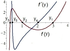
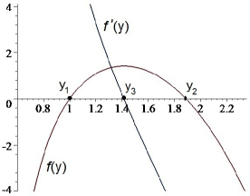
Figure 1: Section 2.1, cases (a) and (b): graphs of functions $f$ and $f^{\prime}$.
(a) $\Psi_{1}>0,\ \Psi_{2}>0,\ \Psi_{3}>0,\ D_{P}>0$; (b) $\Psi_{1}<0,\ \Psi_{2}>0,\ \Psi_{3}<0$ .

(b) Let $\Psi_{3}<0$. The cubic polynomial $P(z)$ has the properties: $P(0)=-\Psi_{2}<0,\ P(\infty)=-\infty$. Its maximal real root $z_{2}$ is an attractor for the heat equation. Note that the condition $D_{P}>0$ and the fact that the maximal root $z_{0}$ of the derivative $P^{\prime}$ is positive imply that $z_{2}>0$ (and $z_{1}>0$ is the minimal positive root of $P$). Indeed, otherwise all the roots of $P$ are negative, hence both roots of $P_{3}^{\prime}$ are negative in contradiction with the assumption. If $\beta>0$, $\Psi_{1}<0$ and $\beta^{2}-3\,\Psi_{1}\Psi_{3}>0$ (the discriminant of $P^{\prime}$ is positive) then both roots of $P^{\prime}(z)=3\,\Psi_{3}z^{2}+2\,\beta z+\Psi_{1}$ are real and the maximal root $z_{0}=\frac{(\beta^{2}-3\Psi_{1}\Psi_{3})^{1/2}-\beta}{3\Psi_{3}}$ is positive. In view of

$$27\,\Psi_{3}^{2}\cdot D_{P}=4(\beta^{2}-3\,\Psi_{1}\Psi_{3})^{3}-(27\,\Psi_{2}\Psi_{3}^{2}+9\,\beta\,\Psi_{1}\Psi_{3}-2\,\beta^{3})^{2},$$

the condition $D_{P}>0$ implies the inequality $\beta^{2}-3\,\Psi_{1}\Psi_{3}>0$. Thus, the conditions

$$\Psi_{1}<0,\quad\Psi_{2}>0,\quad\Psi_{3}<0,\quad\beta>0,\quad D_{P}>0$$

guarantee existence of a stable stationary solution $y_{2}=z_{2}^{2}>0$ (and existence of unstable stationary solution $y_{1}=z_{1}^{2}>0$) of (36), see Fig. 1(b). Note that $f^{\prime\prime}(y)=(6\,\Psi_{3}\,y^{6}+2\,\Psi_{1}\,y^{2}-12\,\Psi_{2})/y^{5}$ is negative for $y>0$. Hence, $f(y)$ is concave for $y>0$, and $f^{\prime}(y)$ is monotone decreasing (with $f^{\prime}(0+)=\infty$ and $f^{\prime}(\infty)=-\infty$) and has one positive root. We conclude that the basin of a single-point attractor $y=y_{2}$ for the semigroup of (36) is the (invariant) set of continuous functions $y(t)>y_{1}$.

(c) Let $\Psi_{3}=0$. Then $P(z)=\beta\,z^{2}+\Psi_{1}\,z-\Psi_{2}$, see (36). A positive root $\tilde{z}$ of $P(z)$ corresponds to a stationary solution $\tilde{y}=\sqrt{\tilde{z}}$ of (36); moreover, if $P\,^{\prime}(\tilde{z})<0$ then $\tilde{y}$ is a single-point attractor.

(c₁) Assume $\beta<0$. We have $P(0)=-\Psi_{2}<0$ and $P(\infty)=-\infty$. Thus, $P(z)$ has real roots if and only if $P(z_{0})>0$, where $z_{0}=-\Psi_{1}/\beta$ is a root of $P^{\prime}(z)=0$. In our case, the inequality $P(z_{0})>0$ is valid when $-(\Psi_{1})^{2}/(4\Psi_{2})<\beta<0$. Maximal root $y_{2}=\big{(}\frac{\Psi_{1}+(\Psi_{1}^{2}-4\,|\beta|\,\Psi_{2})^{1/2}}{2|\beta|}\big{)}^{1/2}$ of $f(y)=0$ is asymptotically stable, but the second (minimal) root $y_{1}$ is unstable; moreover, $f^{\prime}(y)$ has a unique positive root $y_{3}$, and $f^{\prime}(y)$ takes minimum at $y_{4}$, see Fig. 2. If $-4\,\beta\Psi_{2}=\Psi_{1}^{2}$ then (36) has one positive stationary solution, and has no stationary solutions if $-4\,\beta\Psi_{2}>\Psi_{1}^{2}$.

(c₂) Let $\beta>0$. We have $P(0)=-\Psi_{2}<0$ and $P(\infty)=\infty$. Thus, $P(z)$ has one positive root $z_{2}$, which corresponds to unstable stationary solution of (36), because $P^{\prime}(z_{2})>0$. One may show that for $\beta=0$, (36) has a unique positive stationary solution, which is unstable.

(c₃) Let $\Psi_{2}=0$, then $f(y)=\beta\,y+\Psi_{1}y^{-1}$. If $\beta\geq 0$ then there are no positive stationary solutions. If $\beta<0$ and $\Psi_{1}>0$ then $f(y)=0$ has one positive root $y_{2}=({\Psi_{1}/|\beta|})^{1/2}$. The solution $y_{1}$ is stable (attractor) because $f^{\prime}(y_{2})<0$.

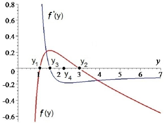
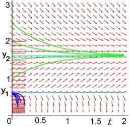
Figure 2: Section 2.1, paragraph (c₁): $P(y^{2})=\beta\,y^{4}+\Psi_{1}\,y^{2}-\Psi_{2}$ with $\beta<0$ and $4\,|\beta|\,\Psi_{2}<\Psi_{1}^{2}$.
(a) Graphs of $f$ and $f^{\prime}$ for $\Psi_{3}=0$, $\Psi_{1}>0$, $\Psi_{2}>0$.   (b) $y_{1}$ is unstable, and $y_{2}$ is stable.

2.2 A fixed point of a one-parametric semigroup

Definition 1.

Let $(X,\,d)$ and $(Y,\,d^{\,\prime})$ be metric spaces. A family of mappings $\{f_{\alpha}:\,X\rightarrow Y\}_{\alpha\in\mathcal{A}}$ is called equicontinous, if for any $\varepsilon>0$ there is $\delta>0$ such that for any pair of points $x_{1},x_{2}\in X$ satisfying the condition $d(x_{1},x_{2})<\delta$ the inequality $d^{\,\prime}(f_{\alpha}(x_{1}),f_{\alpha}(x_{2}))<\varepsilon$ holds for any $\alpha\in\mathcal{A}$. A family of mappings $\{f_{t}:\,X\rightarrow Y\}_{t\in[a,\,b]}$ is called continuous by $t$ uniformly with respect to $x\in X$, if the family of mappings $\{\phi_{x}(t):=f_{t}(x):\,[a,\,b]\rightarrow Y\}_{x\in X}$ is equicontinuous.

The following lemma extends the Arzela-Ascoli Theorem.

Lemma 2.

Let $\mathcal{U}=\{u_{\alpha}\}_{\alpha\in\mathcal{A}}$ be a family of functions defined in a closed interval $[a,\,b]$, with values in a Banach space $E$ and having the properties:

$(a)$ for any $t\in[a,\,b]$ the set $U_{t}=\{u_{\alpha}(t)\}_{\alpha\in\mathcal{A}}$ is precompact in $E$;

$(b)$ the family $\mathcal{U}$ is equicontinuous.

Then the family $\mathcal{U}$ is precompact in $C([a,\,b],\,E)$.

Proof. For any $n\in\mathbb{N}$ consider on $[a,\,b]$ the grid $t_{k}=a+\frac{k}{n}(b-a)\;(k=0,1,\dots,n)$ and the set $\mathcal{U}_{n}$ of all functions $u\in C([a,\,b],\,E)$ having the properties:

– for any $k\in\{0,1,\dots,n\}\;$ $u(t_{k})\in U_{t_{k}}$;

– $u(t)$ is linear in each interval $[t_{k},\,t_{k+1}]$, i.e., $u(t)=n(t_{k+1}-t)u(t_{k})+n(t-t_{k})u(t_{k+1})$.

It is easy to see that each set $\mathcal{U}_{n}$ is homeomorphic to the product $U_{t_{0}}\times U_{t_{1}}\times\dots\times U_{t_{n}}$; hence, and in view of (a), it is precompact in $C([a,\,b],\,E)$. On the other hand, (b) easily implies that for any $\varepsilon>0$ it is possible to choose $n\in\mathbb{N}$ such that $\|u-u_{n}\|_{C([a,\,b],\,E)}<\varepsilon$ for any $u\in\mathcal{U}\;$, where $u_{n}$ is a function from $\mathcal{U}_{n}$ such that $u_{n}(t_{k})=u(t_{k})\;(k=0,1,\dots,n)$. So, for any $\varepsilon>0$, the set $\mathcal{U}$ has a precompact $\varepsilon$-net in $C([a,\,b],\,E)\;$; hence, it is precompact in $C([a,\,b],\,E)$. ∎

Lemma 3.

Let $\{u_{n}(t)\}_{n=1}^{\infty}$ be a sequence of continuous functions, defined in a closed interval $[a,\,b]$, with values in a Banach space $E$ and having the following properties:

$(a)$ there exists a sequence $\tau_{n}>0$ such that $\lim_{\,n\rightarrow\infty}\tau_{n}=0$ and $u_{n}(t+\tau_{n})=u_{n}(t)$ if $\,t,\,t+\tau_{n}\in[a,\,b]$;

$(b)$ the sequence $\{u_{n}(t)\}_{n=1}^{\infty}$ converges uniformly in $[a,\,b]$ to a function $u:[a,\,b]\to Y$.

Then $u(t)$ is constant.

Proof. By (b), the sequence $\{u_{n}(t)\}_{n=1}^{\infty}$ is equicontinuous, i.e., for any $\varepsilon>0$ there exists $\delta>0$ such that $|t-s|<\delta\,(t,\,s\in[a,\,b])$ implies $\|u_{n}(t)-u_{n}(s)\|_{E}<\varepsilon/3$ for any $n\in\mathbb{N}$. By conditions, we can choose $N>0$ such that $\tau_{n}\leq\delta$ and $|u(t)-u_{n}(t)|<\varepsilon/3$ for any $n\geq N$ and $t\in[a,\,b]$. Let us take $a\leq t_{1}<t_{2}\leq b$. In view of (a), $u_{n}(t_{1})=u_{n}(t_{1}+k_{n}\tau_{n})$, where $k_{n}=\Big{[}\frac{t_{2}-t_{1}}{\tau_{n}}\Big{]}$. Observe that $0\leq t_{2}-t_{1}-k_{n}\tau_{n}<\tau_{n}$. The above arguments imply

$$\|u(t_{2})-u(t_{1})\|_{E}\leq\|u(t_{2})-u_{n}(t_{2})\|_{E}+\|u(t_{1})-u_{n}(t_{1})\|_{E}+\|u_{n}(t_{2})-u_{n}(t_{1}+k_{n}\tau_{n})\|_{E}<\varepsilon$$

for $n\geq N$. Since $\varepsilon>0$ is arbitrary, this proves the claim. ∎

Now we turn to the main result of this section. A mapping $f:X\to Y$ between metric spaces is called compact if it is continuous and maps each bounded set in $X$ onto a precompact set in $Y$.

Theorem 6.

Let $G$ be a closed bounded convex subset of a Banach space $E$. Suppose that a one-parametric semigroup of mappings $\{S_{t}:G\to G\,\}_{t\geq 0}$ has the properties:

$(a)$ for any $t>0$ the mapping $S_{t}$ is compact;

$(b)$ for any $\;0<a<b$ the family of mappings $S_{t}$ is continuous by $t$ in the segment $[a,\,b]$

uniformly w.r.t. $u\in G$.

Then the semigroup $\{S_{t}\}_{t\geq 0}$ has in $G$ a common fixed point.

Proof. Shauder’s Fixed Point Theorem claims that a compact mapping of a closed bounded convex set $G$ in a Banach space $E$ into itself has a fixed point, see [2, p. 74]. By $(a)$ and Shauder’s Fixed Point Theorem, for any $\tau>0$ the mapping $S_{\tau}$ has a fixed point $u_{\tau}^{0}\in G$, i.e., $S_{\tau}u_{\tau}^{0}=u_{\tau}^{0}$. In view of the semigroup property $S_{t}\circ S_{\tau}=S_{t+\tau}$, the function $u_{\tau}(t)=S_{t}u_{\tau}^{0}$ is $\tau$-periodic. Take a sequence of positive numbers $\{\tau_{n}\}_{n=1}^{\infty}$ such that $\lim\limits_{\,n\rightarrow\infty}\tau_{n}=0$, and denote $u_{n}(t)=u_{\tau_{n}}(t)$, $u_{n}^{0}=u_{\tau_{n}}^{0}$. By conditions, the sequence of functions $\{u_{n}(t)\}_{n=1}^{\infty}$ satisfies on $[a,\,b]$ assumptions of Lemma 2; hence, it is precompact in $C([a,\,b],\,E)$. Thus, it is possible to select from the sequence $u_{n}(t)$ a subsequence $u_{n_{k}}(t)$ converging to a function $u(t)$ in the $C([a,\,b],\,E)$-norm. Applying Lemma 3 to this subsequence, we find that $u(t)$ is constant, i.e., $u(t)\equiv u_{*}$ in $[a,\,b]$. Since $u_{n_{k}}(t)\in G$ for any fixed $t\in[a,\,b]$ and $G$ is closed in $E$, we obtain $u_{*}\in G$. Since $u_{n_{k}}(t)=S_{t-a}u_{n_{k}}(a)\;(t\in[a,\,b])$ and the mappings $S_{t}:\,G\rightarrow G$ are continuous, we get, tending $k\rightarrow\infty$, that $S_{t-a}u_{*}=u_{*}$ for any $t\in[a,\,b]$. ∎

2.3 Solutions of the nonlinear heat equation

In this section we investigate the existence of solutions of a semi-linear elliptic equation. For this we prove existence of global solutions of associated non-linear parabolic equation and study its stable stationary solutions. We reduce this problem to the existence of a common fixed point for the one-parameter semigroup of mappings, see Theorem 6, corresponding to the non-linear parabolic equation. Some results of this section may be known, but for convenience of a reader, we give the proofs.

2.3.1 Global solutions

Let $(F,g)$ be a closed Riemannian manifold. Define a bounded, closed and convex set in $C(F)$ by

$$G=\{u\in C(F):\ u_{-}(x)\leq u(x)\leq u_{+}(x)\ \ {\rm for\ all}\ \ x\in F\},$$ (38)

where $u_{-},u_{+}\in C(F)$, $u_{-}\leq u_{+}$, and the following compact domain in $\mathbb{R}\times F$ by:

$$D:=\{(u,\,x)\in\mathbb{R}\times F:\;u_{-}(x)\leq u\leq u_{+}(x)\}.$$ (39)

Consider the Cauchy’s problem for a non-linear heat equation, more general than (31),

$$\partial_{t}u=\Delta u+{f}(u,x),\quad u(x,0)=u_{0}(x)\in C(F)\,,$$ (40)

where ${f}\in C(D)$, and the stationary version of equation (40)₁:

$$\Delta u+{f}(u,x)=0.$$ (41)

Definition 2.

A function $u(x,t)$ is a solution of (40) in the domain $F\times[0,T]$, if it is continuous, satisfies the initial condition (40)₂, and in $F\times(0,T]$ it is continuously differentiable by $t$, twice continuously differentiable by $x$ and satisfies (40)₁. A function $u(x)$ is a solution of (41) in $F$, if it belongs to $C^{2}(F)$ and satisfies this equation in $F$.

Let $S_{t}:C(F)\rightarrow C(F)$ be the map which relates to each initial value $u_{0}\in C(F)$ the value of the classical solution of (40) at the moment $t\in[0,T)$ (if this solution exists and is unique). Since ${f}(u,x)$ does not depend explicitly on $t$, the family $\{S_{t}\}_{0\leq t<T}$ has the semigroup property, and it is a semigroup (i.e., $T=\infty$) when (40) admits a global solution for any $u_{0}(x)\in C(F)$.

It is known, see [4, Theorem B.6.3], that the Cauchy’s problem for the heat equation,

$$\partial_{t}v=\Delta v,\quad v(x,0)=v_{0}(x)$$ (42)

admits a unique global solution $v(x,t)$ for any $v_{0}\in C(F)$. Let $S_{t}^{0}:\,C(F)\rightarrow C(F)\ (t\geq 0)$ be the semigroup of linear mappings corresponding to (42). Since $v(x,t)$ is continuous in $F\times[0,T]$ then $S_{t}^{0}v_{0}\to v_{0}$ in the $C(F)$-norm as $t\downarrow 0$. This means that the semigroup $\{S_{t}^{0}\}$ is strongly continuous in $C(F)$. It is known that

$$v(x,t)=(S_{t}^{0}v_{0})(x)=\int_{F}H(x,y,t)\,v_{0}(y)\,dy,$$ (43)

where $H(x,y,t)$ is the fundamental solution of (42)₁, called the heat kernel, which belongs to $C^{\infty}(\Omega)$ in the domain $\Omega:=F\times F\times\{t\in\mathbb{R}:\,t>0\}$, see [4]. We shall use the properties

$$H(x,\xi,t)>0,\quad\int_{F}H(x,\xi,t)\,{\rm d}\xi=1\quad(x\in F,\ t>0).$$ (44)

If a solution of (40) exists then it satisfies the integral equation (Duhamel’s principle):

$$u(x,t)=\int_{F}H(x,y,t)\,u_{0}(y)\,{\rm d}y+\int_{0}^{t}\int_{F}H(x,y,t-\tau)\,{f}(u(y,\tau),y)\,{\rm d}y\operatorname{d}\!\tau\,.$$ (45)

Denote by $\mathbb{T}$ the set of all $T>0$ such that (45) has a continuous solution in the domain $F\times[0,T]$. For $u_{0}\in\mathrm{Int}(G)$ and $r>0$, let $B_{r}(u_{0})=\{u\in C(F):\,\|u-u_{0}\|_{C(F)}\leq r\}$ be a closed ball contained in $G$. One may take $r=\min\{\min_{\,F}|u_{0}-u_{-}|,\ \min_{\,F}|u_{0}-u_{+}|\}$.

Proposition 3.

If $q\in C^{\infty}(D)$ and $u_{0}\in\mathrm{Int}(G)$ then

$(i)$ $\mathbb{T}\neq\emptyset$, namely, there are $T>0$ and $r>0$ such that the integral equation (45) has a unique continuous solution $u(x,t)$ in $F\times[0,T]$, with the property $u(\cdot\,,t)\in B_{r}(u_{0})$ for any $t\in(0,T]$;

$(ii)$ for any $T\in\mathbb{T}$, a continuous solution $u(x,t)$ of (45) in the domain $F\times[0,T]$ is a solution of (40). Moreover, $u(\cdot,\cdot)\in C^{\infty}(F\times(0,T])$;

$(iii)$ for any $T\in\mathbb{T}$, a solution of (40) is unique in $F\times[0,T]$.

Proof. satisfies the Lipschitz condition w.r.t. $u$, i.e., there exists $L>0$ such that

$$|{f}(u_{2},x)-{f}(u_{1},x)|\leq L|u_{2}-u_{1}|\quad\forall\,(u_{1},x)\,,(u_{2},x)\in D.$$ (46)

Hence, the superposition operator $(\mathcal{X}u)(x)={f}(u(x),x)$ satisfies the Lipschitz condition: $\|\mathcal{X}u_{1}-\mathcal{X}u_{2}\|_{C(F)}\leq L\|u_{1}-u_{2}\|_{C(F)}\ (\forall\,u_{1},u_{2}\in G)$. Let $\Theta$ be the operator expressed by the rhs of (45) and defined on the set $C([0,T],B_{r}(u_{0}))$, which is closed in the Banach space $C([0,T],C(F))$. By Lemma 5$(i)$ and the proof of Proposition 1.1 in [14, p. 315], we can choose $T>0$ such that $\Theta$ maps the set $C([0,T],B_{r}(u_{0}))$ into itself and it is a contraction there. Hence, (45) has in $C([0,T],B_{r}(u_{0}))$ a unique solution.

$(ii)$ The proof consists of two steps.

Step 1. Let us show that $u(\cdot,t)\in C^{1}(F)$ for any $t\in(0,T]$. Since $H(\,\cdot\,,\cdot\,,\cdot\,)\in C^{\infty}(\Omega)$, the first integral in (45) belongs to class $C^{\infty}(F\times(0,T])$. It remains to prove that the second integral in (45), denoted by $I_{0}(x,t)$, belongs to $C^{1}(F)$ for any $t\in(0,T]$. Consider the truncated integral $I_{\varepsilon}(x,t)=\int_{0}^{t-\varepsilon}\int_{F}H(x,y,t-\tau)\,{f}(u(y,\tau),y)\,{\rm d}y\operatorname{d}\!\tau$ for $\varepsilon\in(0,t)$. We have

$$|\,I_{\varepsilon}(x,t)-I_{0}(x,t)\,| = \big{|}\int_{t-\varepsilon}^{t}\int_{F}H(x,y,t-\tau)\,{f}(u(y,\tau),y)\,{\rm d}y\operatorname{d}\!\tau\big{|}$$

$$\leq \|{f}(\cdot,\cdot)\|_{C(D)}\int_{t-\varepsilon}^{t}\int_{F}H(x,y,t-\tau)\,{\rm d}y\operatorname{d}\!\tau=\varepsilon\,\|{f}(\cdot,\cdot)\|_{C(D)}.$$

Hence, for any $t\in(0,T]$, the integral $I_{\varepsilon}(x,t)$ converges to $I_{0}(x,t)$ as $\varepsilon\downarrow 0$ uniformly on $F$.

Observe that since $H(\,\cdot\,,\cdot\,,\cdot\,)\in C^{\infty}(\Omega)$, thus $I_{\varepsilon}(\cdot\,,t)\in C^{\infty}(F)$. Hence, in order to prove that $I(\cdot\,,t)\in C^{1}(F)$ for $t>0$, it is sufficient to show that the first order partial derivatives of $I_{\varepsilon}(x,t)$ by all variables converge as $\varepsilon\downarrow 0$ uniformly for any local coordinates $(x_{k})$ with compact support $W$ on $F$. Take $x\in W$ and consider derivatives

$$\partial_{x_{k}}I_{\varepsilon}(x,t)=\int_{0}^{t-\varepsilon}\partial_{x_{k}}\int_{F}H(x,y,t-\tau)\,{f}(u(y,\tau),y)\,{\rm d}y\operatorname{d}\!\tau.$$

Using (43) and estimate $\|S_{t}^{0}\|_{\mathcal{B}(C(F),C^{1}(F))}\leq C\,t^{-1/2}$ with $t\in(0,1]$, see [14, (1.11), p. 315], we have for $0<\varepsilon_{1}<\varepsilon_{2}<t$:

$$|\partial_{x_{k}}I_{\varepsilon_{1}}(x,t)-\partial_{x_{k}}I_{\varepsilon_{2}}(x,t)|\leq\int_{t-\varepsilon_{2}}^{t-\varepsilon_{1}}|\partial_{x_{k}}(S^{0}_{t-\tau}\mathcal{X}(u))(x)|\,\operatorname{d}\!\tau$$

$$\leq C\,\|\mathcal{X}(u)\|_{C(F)}\int_{t-\varepsilon_{2}}^{t-\varepsilon_{1}}(t-\tau)^{-1/2}\,\operatorname{d}\!\tau\leq 2\,C\,\sqrt{\varepsilon_{2}}\,\|{f}(\cdot,\cdot)\|_{C(D)}.$$

This estimate shows us that the following integral exists:

$$J_{k}(x,t):=\int_{0}^{t}\int_{F}\partial_{x_{k}}H(x,y,t-\tau)\,{f}(u(y,\tau),y)\,{\rm d}y\operatorname{d}\!\tau,$$

and $\partial_{x_{k}}I_{\varepsilon}(x,t)\rightarrow J_{k}(x,t)$ as $\varepsilon\downarrow 0$ uniformly on $F$ for any $t\in(0,T]$. Hence, $I(\cdot,t)\in C^{1}(F)$, and, therefore, $u(\cdot,t)\in C^{1}(F)$ for any $t\in(0,T]$.

Step 2. Let us show that $u(\cdot,\cdot)\in C^{\infty}(F\times(0,T])$. Observe that for any $\sigma\in(0,T)$, the restriction of $u(x,t)$ on $F\times[\sigma,T]$ is a solution of the integral equation

$$u(x,t)=\int_{F}H(x,y,t)\,u_{\sigma}(y)\,{\rm d}y+\int_{\sigma}^{t}\int_{F}H(x,y,t-\tau)\,{f}(u(y,\tau),y)\,{\rm d}y\operatorname{d}\!\tau,$$

where $u_{\sigma}(x)=u(x,\sigma)$. By Step 2, $u_{\sigma}\in C^{1}(F)$. Taking into account that ${f}(\cdot,\cdot)\in C^{\infty}(D)$, and using [14, Proposition 1.2, p. 316], we obtain that $u\in C^{\infty}(F\times(\sigma,T])$. Since $\sigma\in(0,T)$ is arbitrary, then $u\in C^{\infty}(F\times(0,T])$. Furthermore, one may conclude from (45), that $u(x,t)$ satisfies initial condition (40)₂, and in the domain $F\times(0,T]$ it obeys (40)₁.

$(iii)$ Assume that (40) has two solutions $u_{1}(x,t)$ and $u_{2}(x,t)$ in the domain $F\times[0,T]$. Then, in view of (46), the function $w(x,t)=u_{2}(x,t)-u_{1}(x,t)$ satisfies the differential inequalities:

$$\Delta w-L|w|\leq\partial_{t}w\leq\Delta w+L|w|.$$

By the maximum principle, $w_{-}(t)\leq w(x,t)\leq w_{-}(t)$, where $w_{-}(t),w_{+}(t)$ solve the problems

$${dw_{-}}/{dt}=-L\,|w_{-}(t)|,\ \ w_{-}(0)=0,\qquad{dw_{+}}/{dt}=-L\,|w_{+}(t)|,\ \ w_{+}(0)=0.$$

Hence, $w(x,t)\equiv 0$ in $F\times[0,T]$. ∎

Theorem 7.

Suppose that $q\in C^{\infty}(D)$ and $u_{0}\in\mathrm{Int}(G)$. If there exist continuous functions $\tilde{u}_{-}(x)$ and $\tilde{u}_{+}(x)$ such that $u_{-}<\tilde{u}_{-}<\tilde{u}_{+}<u_{+}$, and for any $T\in\mathbb{T}$ for the solution $u_{T}(x,t)$ of Cauchy’s problem (40) the estimates $\tilde{u}_{-}(x)\leq u_{T}(x,t)\leq\tilde{u}_{+}(x)$ are valid in the domain $F\times[0,T]$. Then (40) has a global solution $u(x,t)$, i.e., it is defined in the domain $F\times(0,\infty)$. Furthermore, it is unique there and satisfies the inequalities $\tilde{u}_{-}(x)\leq u(x,t)\leq\tilde{u}_{+}(x)$. Moreover, $u(\cdot,\cdot)\in F\times(0,\infty)$.

Proof. By Proposition 3$(i)$, $\mathbb{T}\neq\emptyset$. Denote $\tilde{T}=\sup(\mathbb{T})$. We should prove that $\tilde{T}=\infty$. Assume on the contrary that $\tilde{T}<\infty$. Since by Proposition 3(iii), for any $T\in\mathbb{T}$, $u_{T}(x,t)$ is a unique solution of (40) in $F\times[0,T]$, then we can consider the function $u(x,t)$, defined on $F\times[0,\tilde{T})=\bigcup_{\,T\in\mathbb{T}}F\times[0,T]$ such that for any $T\in\mathbb{T}$ $u_{T}=u|_{F\times[0,T]}$. It is a unique solution of (40) in the domain $F\times[0,\tilde{T})$; hence, it satisfies in this domain the integral equation (45). We have for $(x,t_{k})\in F\times[0,\tilde{T})$ using (44):

$$\big{|}\int_{0}^{t_{2}}\int_{F}H(x,y,t-\tau)\,{f}(u(y,\tau),y)\,{\rm d}y\operatorname{d}\!\tau-\int_{0}^{t_{1}}\int_{F}H(x,y,t-\tau)\,{f}(u(y,\tau),y)\,{\rm d}y\operatorname{d}\!\tau\big{|}$$

$$\leq|t_{2}-t_{1}|\cdot\|{f}(\cdot,\cdot)\|_{C(D)}.$$

This estimate and (45) show us that $u(x,t)$ tends to a continuous function $\tilde{u}(x)$ as $t\uparrow\tilde{T}$ in the $C(F)$-norm. Since $u_{-}(x)<\tilde{u}_{-}(x)\leq u(x,t)\leq\tilde{u}_{+}(x)<u_{+}(x)$ in $F\times[0,\tilde{T})$, then $\tilde{u}\in\mathrm{Int}(G)$. Therefore, by Proposition 3(i)-(ii) there exists $\delta>0$ such that the Cauchy’s problem

$$\partial_{t}v=\Delta u+{f}(v,x),\quad v(x,\tilde{T})=\tilde{u}(x)$$

has a solution $v(x,t)$ in $F\times[\tilde{T},\tilde{T}+\delta]$. It is easy to check that the function

$$w(x,t)=\left\{\begin{array}[]{ll}u(x,t),&\mathrm{if}\quad(x,t)\in F\times[0,\tilde{T}),\\ v(x,t),&\mathrm{if}\quad(x,t)\in F\times[\tilde{T},\tilde{T}+\delta]\end{array}\right.$$

is a continuous solution of the integral equation (45) in $F\times[0,\tilde{T}+\delta]$. This fact contradicts to the definition of the number $\tilde{T}$. Thus, $\tilde{T}=\infty$; hence, $u(x,t)$ is a unique global solution of Cauchy’s problem (40) satisfying in $F\times[0,\infty)$ the estimates $\tilde{u}_{-}(x)\leq u(x,t)\leq\tilde{u}_{+}(x)$. Furthermore, by Proposition 3$(ii)$, $u(\cdot,\cdot)\in C^{\infty}(F\times(0,\infty))$. ∎

2.3.2 Stationary solutions

The proof of the following theorem is supported by Lemmas 4–7 in what follows.

Theorem 8.

Let the following conditions are satisfied:

– ${f}\in C^{\infty}(D)$, for $D$ in (39),

– (40) admits a global solution for any $u_{0}(x)\in G$, and

– the set $G$ is invariant w.r.t. the corresponding semigroup $S_{t}\ (t\geq 0)$.

Then the set of all solutions of (41) lying in $G$ is nonempty and compact in $C(F)$.

Proof. Take $u_{0}\in G$. By the Duhamel’s principle, we have

$$S_{t}u_{0}=S_{t}^{0}u_{0}+\int_{0}^{t}S_{t-\tau}^{0}{f}(S_{\tau}u_{0},\,\cdot)\,\operatorname{d}\!\tau\,,$$ (47)

where $S_{t}^{0}$ is the semigroup associated with (42)₁. Denote by $\|\cdot\|_{\cal{B}(C(F))}$ the operator norm. For any $t\in[a,\,b]\;(0<a<b)$, $\delta\in(0,\,a)$ and $h\in(0,\,\delta)$, we have

$$\hskip-17.07164pt\|u(\cdot,t+h)-u(\cdot,t)\|_{C(F)}\leq\delta\max_{\tau\in[t+h-\delta,\,t+h]}\|S_{t+h-\tau}^{0}\|_{\cal{B}(C(F))}\cdot\|{f}(S_{\tau}u_{0},\,\cdot)\|_{C(F)}$$

$$\hskip-17.07164pt+\,\delta\max_{\tau\in[t-\delta,\,t]}\big{(}\|S_{t-\tau}^{0}\|_{\cal{B}(C(F))}\cdot\|{f}(S_{\tau}u_{0},\,\cdot)\|_{C(F)}\big{)}+\|S_{t+h}^{0}-S_{t}^{0}\|_{\cal{B}(C(F))}\cdot\|u_{0}\|_{C(F)}$$ (48)

$$\hskip-17.07164pt+h\!\max_{\tau\in[t-\delta,t-\delta+h]}\|S_{t+h-\tau}^{0}\|_{\cal{B}(C(F))}\|{f}(S_{\tau}u_{0},\cdot)\|_{C(F)}{+}\max_{\tau\in[0,t-\delta]}\|S_{t+h-\tau}^{0}{-}S_{t-\tau}^{0}\|_{\cal{B}(C(F))}\|{f}(S_{\tau}u_{0},\cdot)\|_{C(F)}.$$

Given any $\varepsilon>0$, by Lemma 5(i), we can choose $\delta>0$ such that the sum of the first two terms in the rhs of (2.3.2) is less than $\varepsilon/2$ for any $u_{0}\in G$. Furthermore, in view of Lemma 5(iii), the family $\{S_{t}^{0}\}$ is uniformly continuous by $t$ in the operator norm on each compact interval which does not contain $t=0$, we can choose $h>0$ such that the sum of the remain terms in the rhs of the last estimate will be less than $\varepsilon/2$ for any $u_{0}\in G$. This means that the semigroup $S_{t}$ is continuous by $t$ in $[a,\,b]$ uniformly w.r.t. $u_{0}\in G$ for any $0<a<b$. Then, in view of the continuity of ${f}(u,x)$ in $D$ and the invariance of $G$ with respect to the semigroup $S_{t}$, the family of mappings $Q_{t}u_{0}:={f}(S_{t}u_{0},\,\cdot)$ is continuous by $t$ in $[a,\,b]$ uniformly w.r.t. $u_{0}\in G$ for any $0<a<b$. These circumstances, equality (47), Lemmas 4, 5(i-ii) and 7(ii) imply that each mapping $S_{t}$ with $t>0$ is compact on $G$. So, $S_{t}$ satisfies all conditions of Theorem 6. Hence, it has in $G$ a common fixed point $u_{*}(x)$, i.e., $S_{t}u_{*}=u_{*}$ for any $t>0$. On the other hand, it is known that for any $u_{0}\in G$ and $t>0$ $S_{t}u_{0}\in C^{\infty}(F)$ (see Proposition 3). Hence $u_{*}(x)$ belongs to $C^{\infty}(F)$ and it is a solution of (41).

By continuity of $S_{t}u_{0}$ by $u_{0}$, the set ${\rm Fix}(G)$ of all common fixed points of $S_{t}\,(t>0)$ in $G$ is closed w.r.t. the $C$-norm. Since $S_{t}({\rm Fix}(G))={\rm Fix}(G)$ for $t>0$, and $S_{t}$ maps any $C$-bounded set on a $C$-precompact set, then ${\rm Fix}(G)$ is $C$-precompact. Thus, ${\rm Fix}(G)$ is $C$-compact. ∎

Lemma 4.

In conditions of Theorem 8, for any $t>0$, the mapping $S_{t}:\,G\rightarrow G$ is continuous.

Proof. Take $u_{1}^{0},u_{2}^{0}\in G$ and denote $u_{k}(x,t)=(S_{t}u_{k}^{0})(x)\;(k=1,2)$. Then, in view of (46), the function $w(x,t)=u_{2}(x,t)-u_{1}(x,t)$ satisfies the differential inequalities:

$$\Delta w-L|w|\leq\partial_{t}w\leq\Delta w+L|w|.$$

Let $w_{-}(t),w_{+}(t)$ be solutions of the following Cauchy’s problems with $w_{0}=\|u_{2}^{0}-u_{1}^{0}\|_{C(F)}$:

$${dw_{-}}/{dt}=-L\,|w_{-}(t)|,\ \ w_{-}(0)=-w_{0},\qquad{dw_{+}}/{dt}=-L\,|w_{+}(t)|,\ \ w_{+}(0)=w_{0}.$$

By the maximum principle, $w_{-}(t)\leq w(x,t)\leq w_{-}(t)$ and $|w(x,t)|\leq w_{0}\,e^{-Lt}$. ∎

Lemma 5.

The semigroup $S_{t}^{0}:\,C(F)\rightarrow C(F)$ has the properties:

$(i)$ $\|S_{t}^{0}\|_{\cal{B}(C(F))}\leq 1$ for any $t\geq 0$;

$(ii)$ the linear operator $S_{t}^{0}$ is compact for any $t>0$;

$(iii)$ the family $S_{t}^{0}$ is continuous by $t\in(0,\,\infty)$ in the operator norm.

Proof. For $v_{0}\in C(F)$ denote $v(x,t)=(S_{t}^{0}v_{0})(x)$ . By (43) and (44), we get for $x,\,y\in F$, $t>0$:

$$|v(x,t)|\leq\|v_{0}\|_{C(F)},$$ (49)

$$|v(x,t)-v(y,t)|\leq{\rm Vol}(F)\sup\nolimits_{\,\xi\in F}|H(x,\xi,t)-H(y,\xi,t)|\cdot\|v_{0}\|_{C(F)}.$$ (50)

Thus, (49) implies $(i)$.

Consider the unit ball $B_{1}=\{f\in C(F):\|f\|_{C(F)}\leq 1\}$ in $C(F)$. Estimates (49), (50) and continuity of the heat kernel $H(x,\xi,t-\tau)$ on each compact of the form $K_{\delta}=F\times F\times\{(t,\,\tau):\;0\leq\tau\leq t-\delta\}\;(\delta>0)$ imply that for $t>0$ the set $S_{t}^{0}(B_{1})$ is bounded in $C(F)$ and it is equicontinuous. By the Arzela-Ascoli Theorem, it is precompact in $C(F)$. This proves $(ii)$.

Let us prove $(iii)$. As above, put $v(x,t)=(S_{t}^{0}v_{0})(x)$. For $t_{1},\,t_{2}\in(0,\,\infty)$ and $x\in F$ we get

$$|v(x,t_{1})-v(x,t_{2})|\leq{\rm Vol}(F)\sup\nolimits_{\,\xi\in F}|H(x,\xi,t_{1})-H(x,\xi,t_{2})|\cdot\|v_{0}\|_{C(F)}.$$

This estimate and the continuity of the heat kernel on each compact $K_{\delta}$, imply $(iii)$. ∎

Lemma 6.

Let $\{T_{n}\}_{n=1}^{\infty}$ be a set of compact mappings acting from a bounded subset $B$ of a Banach space $E_{1}$ into a Banach space $E_{2}$ and converging uniformly to $T:B\rightarrow E_{2}$. Then $T$ is compact.

Proof. The continuity of $T$ is obvious. Take an arbitrary $\varepsilon>0$ and choose $n\in\mathbb{N}$ such that $\sup_{\,x\in B}\|Tx-T_{n}x\|_{E_{2}}<\varepsilon$. This means that the set $T_{n}(B)$ forms a precompact $\varepsilon$-net for the set $T(B)$ in $E_{2}$. Hence the set $T(B)$ is precompact in $E_{2}$. ∎

Lemma 7.

Let $\{T_{t}\}_{t\in[a,\,b)}$ be a family of compact mappings acting from a bounded subset $B$ of a Banach space $E_{1}$ into a Banach space $E_{2}$.

$(i)$ If $c\in(a,\,b)$ and $T_{t}$ is continuous by $t$ on $[a,\,c]$ uniformly w.r.t. $x\in B$ then the mapping $J^{c}x:=\int_{a}^{c}T_{t}x\,{\rm d}t\ (x\in B)$ is compact;

$(ii)$ If the condition of $(i)$ is satisfied for any $c\in(a,\,b)$ and the family $J^{c}$ converges as $c\uparrow b$ to the mapping $Jx=\int_{a}^{b}T_{t}x\,{\rm d}t$ uniformly w.r.t. $x\in B$ then $J$ is compact.

Proof. ($i$) For any $n\in\mathbb{N}$ consider on $[a,\,c]$ the grid $t_{k}=a+\frac{k}{n}(c-a)\;(k=1,2,\dots,n)$ and the mapping $J^{c}_{n}x=\frac{1}{n}(c-a)\sum_{\,k=1}^{n}T_{t_{k}}x\;(x\in B)$. One may show that each $J^{c}_{n}$ is compact and the sequence $\{J^{c}_{n}\}_{n=1}^{\infty}$ converges to the mapping $T$ uniformly. By Lemma 6, $T$ is compact. Thus, $(ii)$ follows from $(i)$ and Lemma 6. ∎

2.4 Attractors of the nonlinear heat equation

This section studies stable stationary solutions of (31) for three cases.

2.4.1 Case of $\Psi_{3}>0$

Let $\Psi_{3}>0$, $\Psi_{1}>0$, $\Psi_{2}>0$ and $\lambda_{0}>0$, see Section 2.1, case (a). For $y>0$, put

$$\phi(y,\theta)=-\lambda_{0}\,y+\theta_{1}\,y^{-1}-\theta_{2}\,y^{-3}+\theta_{3}\,y^{3}=P_{\,\phi}(y^{2})/y^{3},$$

where $P_{\,\phi}(z)=\theta_{3}z^{3}-\lambda_{0}z^{2}+\theta_{1}z-\theta_{2}$ and $\theta=(\theta_{1},\theta_{2},\theta_{3})\in\mathcal{P}$. Then $\phi_{-}(y)\leq\phi(y,\theta)\leq\phi_{+}(y)$ for

$$\phi_{+}(y)=-\lambda_{0}y+\Psi_{1}^{+}y^{-1}-\Psi_{2}^{-}y^{-3}+\Psi_{3}^{+}y^{3},\quad\phi_{-}(y)=-\lambda_{0}y+\Psi_{1}^{-}y^{-1}-\Psi_{2}^{+}y^{-3}+\Psi_{3}^{-}y^{3}.$$

The discriminant of $P_{\,\phi}(z)$ is the following cubic polynomial in $\lambda_{0}$:

$$D(P_{\phi})(\lambda_{0})=-4\,\theta_{2}\lambda_{0}^{3}+\theta_{1}^{2}\lambda_{0}^{2}+18\,\theta_{1}\theta_{2}\theta_{3}\lambda_{0}-\theta_{3}(4\,\theta_{1}^{3}+27\,\theta_{2}^{2}\theta_{3})\,.$$ (51)

If $D(P_{\phi})>0$ for some $\lambda_{0}>0$ then $P_{\phi}(z)$ has 3 real roots $z_{3}(\theta)<z_{2}(\theta)<z_{1}(\theta)$, and $y_{k}=z^{2}_{k}\ (k=1,2,3)$ are roots of $\phi(y,\,\cdot)$. Since $P_{\phi}(z)<0$ for $z<0$, all its roots are positive.

By Maclaurin method, positive $\lambda_{0}$-roots of $D(P_{\phi})$ are bounded above by

$$1+\max\{\,\theta_{1}^{2},\ 18\,\theta_{1}\theta_{2}\theta_{3}\,\}/(4\,\theta_{2})\leq K:=1+\max\{\,(\Psi_{1}^{+})^{2},\ 18\,\Psi_{1}^{+}\Psi_{2}^{+}\Psi_{3}^{+}\,\}/(4\,\Psi_{2}^{-}).$$

Since $D(P_{\phi})(-\infty)=\infty$ and $D(P_{\phi})(0)<0$ for any $\theta\in\mathcal{P}$, there is one negative root. Indeed, by Vieta’s formulas, the sum of $\lambda_{0}$-roots is $\theta_{1}^{2}/(4\theta_{2})>0$; hence, three negative roots are impossible.

The discriminant by $\lambda_{0}$ of $D(P_{\phi})$ is $16\,\theta_{3}(\theta_{1}^{3}-27\,\theta_{2}^{2}\theta_{3})^{3}$. If $\theta_{1}^{3}<27\,\theta_{2}^{2}\theta_{3}$ then $D(P_{\phi})$ has one real $\lambda_{0}$-root, which as was shown is negative; this case in not useful for us, because $D(P_{\phi})<0$ for $\lambda_{0}>0$. If $\theta_{1}^{3}>27\,\theta_{2}^{2}\theta_{3}$ then $D(P_{\phi})$ has three real $\lambda_{0}$-roots: one negative and other two positive, $\lambda^{+}(\theta)>\lambda^{-}(\theta)$; moreover, $D(P_{\phi})>0$ when $\lambda_{0}\in I_{\lambda}(\theta)=(\lambda^{-}(\theta),\,\lambda^{+}(\theta))$, Fig. 3(a). In this case, $\phi(y,\theta)$ has three positive roots $y_{1}(\theta)>y_{2}(\theta)>y_{3}(\theta)$, $\partial_{y}\phi(y,\theta)$ has two positive roots $y_{4}(\theta)\in(y_{2}(\theta),\,y_{1}(\theta))$ and $y_{5}(\theta)\in(y_{3}(\theta),\,y_{2}(\theta))$. Thus, in what follows we assume

$$(\Psi^{-}_{1})^{3}>27\,(\Psi^{+}_{2})^{2}\Psi^{+}_{3}.$$ (52)

Since ${\cal P}$ is compact, there exist $\Lambda^{-}=\max_{\,\cal P}\lambda^{-}(\theta)$ and $\Lambda^{+}=\min_{\,\cal P}\lambda^{+}(\theta)$.

Denote by $y_{3}^{+}<y_{2}^{+}<y_{1}^{+}$ the positive roots of $\phi_{+}(y)$, by $y_{3}^{-}<y_{2}^{-}<y_{1}^{-}$ the positive roots of $\phi_{-}(y)$, and $y_{5}^{-}<y_{4}^{-}$ and $y_{5}^{+}<y_{4}^{+}$, respectively, the positive roots of functions

$$(\partial_{y}\phi)_{-}(y)=-\lambda_{0}-\Psi_{1}^{+}y^{-2}+3\Psi_{2}^{-}y^{-4}+3\Psi_{3}^{-}y^{2},$$

$$(\partial_{y}\phi)_{+}(y)=-\lambda_{0}-\Psi_{1}^{-}y^{-2}+3\Psi_{2}^{+}y^{-4}+3\Psi_{3}^{+}y^{2}.$$

We calculate $\partial_{y}\phi(y,\theta)=-\lambda_{0}-\theta_{1}y^{-2}+3\,\theta_{2}y^{-4}+3\,\theta_{3}y^{2}$. For any $\theta\in\mathcal{P}$ and $y>0$ we have

$$(\partial_{y}\phi)_{-}(y)\leq(\partial_{y}\phi)(y,\theta)\leq(\partial_{y}\phi)_{+}(y).$$ (53)

We need the following condition:

$$3\,\Psi^{-}_{3}>\Psi^{+}_{3}.$$ (54)

Proposition 4.

If (52) holds then, for any $\theta\in\mathcal{P}$ and $\lambda_{0}\in I_{\lambda}(\theta)$, we have

$$y_{3}^{+}\leq y_{2}(\theta)\leq y_{3}^{-},\quad y_{2}^{-}\leq y_{2}(\theta)\leq y_{2}^{+},\quad y_{1}^{+}\leq y_{1}(\theta)\leq y_{1}^{-},$$

$$y_{5}^{-}\leq y_{5}(\theta)\leq y_{5}^{+},\quad y_{4}^{-}\leq y_{4}(\theta)\leq y_{4}^{+}.$$

If, in addition, (59), (54) and

$$\delta_{3}^{2}\leq\min\!\Big{\{}1,\frac{8\Psi_{3}^{-}D_{P^{-}}}{27(\Psi_{2}^{+})^{2}{+}18(4\Psi_{1}^{-}\Psi_{2}^{+}\lambda_{0}{+}(\Psi_{1}^{-})^{3}{+}9(\Psi_{2}^{+})^{2}\Psi_{3}^{-})},\frac{(3\,\Psi_{3}^{-}-\Psi_{3}^{+})D_{P^{+}}}{9(4\Psi_{1}^{+}\Psi_{2}^{-}\lambda_{0}{+}(\Psi_{1}^{+})^{3}{+}9(\Psi_{2}^{-})^{2}\Psi_{3}^{+})}\Big{\}}$$ (55)

hold for any $\lambda_{0}\in(\Lambda^{-}+\varepsilon,\,\Lambda^{+}-\varepsilon)$ and some positive $\varepsilon<\frac{1}{2}\,(\Lambda^{+}-\Lambda^{-})$ then

$$y_{3}^{+}<y_{3}^{-}<y_{5}^{+}<y_{2}^{-}<y_{2}^{+}<y_{4}^{-}<y_{1}^{+}<y_{1}^{-}\,.$$ (56)

Proof. For implicit derivatives $\partial_{\theta_{k}}y_{l}=-({\partial_{\theta_{k}}\phi}/{\partial_{y}\phi})\,|_{\,y=y_{l}(\theta)}$, $\partial_{\theta_{k}}y_{j}=-({\partial\,^{2}_{\theta_{k}y}\phi}/{\partial\,^{2}_{yy}\phi})\,|_{\,y=y_{j}(\theta)}$ where $k,l=1,2,3,\ j=4,5$, we calculate

$$\partial_{\theta_{1}}\phi(y,\theta)=y^{-1},\quad\partial_{\theta_{2}}\phi(y,\theta)=-y^{-3},\quad\partial_{\theta_{3}}\phi(y,\theta)=y^{3},$$

$$\partial_{y}\phi|_{y=y_{1}(\theta)}>0,\ \ \partial_{y}\phi|_{y=y_{2}(\theta)}<0,\ \ \partial_{y}\phi|_{y=y_{3}(\theta)}>0,\ \ \partial^{2}_{yy}\phi|_{y=y_{4}(\theta)}>0,\ \ \partial^{2}_{yy}\phi|_{y=y_{5}(\theta)}<0,$$

$$\partial^{2}_{\theta_{1}y}\phi(y,\theta)=-y^{-2},\quad\partial^{2}_{\theta_{2}\,y}\phi(y,\theta)=3\,y^{-4},\quad\partial^{2}_{\theta_{3}y}\phi(y,\theta)=3\,y^{2}\,,$$

where $\partial^{2}_{yy}\phi(y,\theta)=2\,\theta_{1}y^{-3}-12\,\theta_{2}y^{-5}+6\,\theta_{3}y$. Thus, the following inequalities hold:

$$\partial_{\theta_{1}}y_{1}(\theta)<0,\quad\partial_{\theta_{1}}y_{2}(\theta)>0,\quad\partial_{\theta_{1}}y_{3}(\theta)<0,\quad\partial_{\theta_{1}}y_{4}(\theta)>0,\quad\partial_{\theta_{1}}y_{5}(\theta)<0,$$

$$\partial_{\theta_{2}}y_{1}(\theta)>0,\quad\partial_{\theta_{2}}y_{2}(\theta)<0,\quad\partial_{\theta_{2}}y_{3}(\theta)>0,\quad\partial_{\theta_{2}}y_{4}(\theta)<0,\quad\partial_{\theta_{2}}y_{5}(\theta)>0,$$

$$\partial_{\theta_{3}}y_{1}(\theta)<0,\quad\partial_{\theta_{3}}y_{2}(\theta)>0,\quad\partial_{\theta_{3}}y_{3}(\theta)<0,\quad\partial_{\theta_{3}}y_{4}(\theta)<0,\quad\partial_{\theta_{3}}y_{5}(\theta)>0.$$

The first claim follows from the above, see also Section 2.1, case (a). The proof of the second claim is divided into three parts: 1) $\Lambda^{-}<\Lambda^{+}$, 2) $y_{3}^{-}<y_{5}^{+}<y_{2}^{-}\,$, and 3) $y_{2}^{+}<y_{4}^{-}<y_{1}^{+}\,$.

1. Changing variables, $\lambda_{0}=\mu+\theta_{1}^{2}/(12\,\theta_{2})$, we reduce $D(P_{\phi})$ of (51) to depressed form $P(\mu)=\mu^{3}+p(\theta)\,\mu+q(\theta)$, where

$$p(\theta)=-\theta_{1}(\theta_{1}^{3}+216\,\theta_{2}^{2}\theta_{3})/(48\,\theta_{2}^{2})<0,\quad q(\theta)=-(\theta_{1}^{6}-540\,\theta_{2}^{2}\theta_{3}\theta_{1}^{3}-5832\,\theta_{2}^{4}\theta_{3}^{2})/(864\,\theta_{2}^{3}).$$

Due to trigonometric solution of $P(\mu)=0$, three real roots are

$$\mu_{1}(\theta)=A\cos\varphi>0,\quad\mu_{2}(\theta)=A\cos(\varphi-2\pi/3),\quad\mu_{3}(\theta)=A\cos(\varphi+2\pi/3)<0,$$ (57)

where the amplitude is $A=2\,(-p/3)^{1/2}>0$ and the angle variable is given by $\cos(3\,\varphi)=-{4q(\theta)}/{A^{3}}$. Introducing $z={\theta_{3}\theta_{2}^{2}}/{\theta_{1}^{3}}\in[0,\frac{1}{27})$, we obtain a decreasing (from 1 to -1) function in one variable, $\cos(3\,\varphi)=C(z):=-\frac{5832\,z^{2}+540\,z-1}{(216\,z+1)^{3/2}}$, see Fig. 3(b). Hence, there is a unique $\varphi=\frac{1}{3}\arccos C(z)\in[0,\frac{\pi}{3})$. Since $\cos(\varphi+2\pi/3)<\cos(\varphi-2\pi/3)<\cos\varphi$, the roots (57) are ordered as $\mu_{1}(\theta)>\mu_{2}(\theta)>\mu_{3}(\theta)$.

Two positive roots $\lambda^{-}(\theta)<\lambda^{+}(\theta)$ of $D(P_{\phi})$ are given by $\lambda^{-}(\theta)=\mu_{2}(\theta)+\frac{\theta_{1}^{2}}{12\,\theta_{2}}$ and $\lambda^{+}(\theta)=\mu_{1}(\theta)+\frac{\theta_{1}^{2}}{12\,\theta_{2}}$. By (52), we obtain $0\leq z^{-}\leq z\leq z^{+}<\frac{1}{27}$ and $0\leq\varphi^{-}\leq\varphi\leq\varphi^{+}<\frac{\pi}{3}$, where

$$z^{+}=\Psi_{3}^{+}(\Psi_{2}^{+})^{2}/(\Psi_{1}^{-})^{3},\ \ z^{-}=\Psi_{3}^{-}(\Psi_{2}^{-})^{2}/(\Psi_{1}^{+})^{3},\quad 3\,\varphi^{+}=\arccos C(z^{+}),\ \ 3\,\varphi^{-}=\arccos C(z^{-}).$$

Thus, $\mu_{k}^{-}\leq\mu_{k}(\theta)\leq\mu_{k}^{+},\ (k=1,2,3)$, where $A^{\pm}=2\,(-p^{\mp}/3)^{1/2}$ and $\mu_{1}^{\pm}=A^{\pm}\cos\varphi^{\mp}$,

$$\hskip-14.22636pt\mu_{2}^{+}{=}\Big{\{}\begin{array}[]{c}\!A^{+}\cos\big{(}\varphi^{+}{-}\frac{2\,\pi}{3}\big{)}\ {\rm if}\ \cos\big{(}\varphi^{+}{-}\frac{2\,\pi}{3}\big{)}>0,\\ \!A^{-}\cos\big{(}\varphi^{+}{-}\frac{2\,\pi}{3}\big{)}\ {\rm if}\ \cos\big{(}\varphi^{+}{-}\frac{2\,\pi}{3}\big{)}<0,\end{array}\ \mu_{2}^{-}{=}\Big{\{}\begin{array}[]{c}\!A^{-}\cos\big{(}\varphi^{-}{-}\frac{2\,\pi}{3}\big{)}\ {\rm if}\ \cos\big{(}\varphi^{-}{-}\frac{2\,\pi}{3}\big{)}>0,\\ \!A^{+}\cos\big{(}\varphi^{-}{-}\frac{2\,\pi}{3}\big{)}\ {\rm if}\ \cos\big{(}\varphi^{-}{-}\frac{2\,\pi}{3}\big{)}<0,\end{array}$$

$$p^{+}=-\frac{\Psi_{1}^{-}}{48\,(\Psi_{2}^{+})^{2}}\,((\Psi_{1}^{-})^{3}+216\,(\Psi_{2}^{-})^{2}\Psi_{3}^{-}),\quad p^{-}=-\frac{\Psi_{1}^{+}}{48\,(\Psi_{2}^{-})^{2}}\,((\Psi_{1}^{+})^{3}+216\,(\Psi_{2}^{+})^{2}\Psi_{3}^{+}).$$

Finally, $\lambda^{-}(\theta)\leq\mu_{2}^{+}+\frac{(\Psi_{1}^{+})^{2}}{12\,\Psi_{2}^{-}}$ and $\lambda^{+}(\theta)\geq\mu_{1}^{-}+\frac{(\Psi_{1}^{-})^{2}}{12\,\Psi_{2}^{+}}$. To establish $\Lambda^{-}<\Lambda^{+}$, we need to show

$$(\Psi_{1}^{+})^{2}/(12\,\Psi_{2}^{-})-(\Psi_{1}^{-})^{2}/(12\,\Psi_{2}^{+})<\mu_{1}^{-}-\mu_{2}^{+}.$$ (59)

The lhs of (59) tends to 0, when $\delta_{i}\geq 0$ are small enough, while rhs of (59) tends to a positive constant (estimates may be obtained using trigonometric series). In this case, $\Lambda^{-}<\Lambda^{+}$, and there exists $K\in(0,(\Lambda^{+}-\Lambda^{-})/2)$ such that $D(P_{\phi})$ is positive for all $\lambda_{0}\in(\Lambda^{-}+K,\,\Lambda^{+}-K)$ and $\theta\in{\cal P}$.

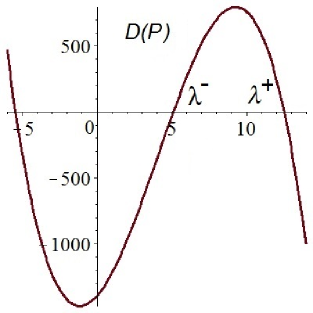
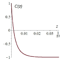
Figure 3: (a) Roots of $D(P_{\phi})$. (b) Graph of $C(z)$ for $0\leq z\leq 1/27\approx 0.037$.

2. Consider the functions

$$\phi_{-}(y) = P_{\,\phi_{-}}(y^{2})/y^{3},\ \ {\rm where}\ \ P_{\,\phi_{-}}(z)=\Psi_{3}^{-}z^{3}-\lambda_{0}\,z^{2}+\Psi_{1}^{-}z-\Psi_{2}^{+},$$

$$\partial_{y}(\phi_{-})(y) = P_{\,\partial_{y}(\phi_{-})}(y^{2})/y^{4},\ \ {\rm where}\ \ P_{\,\partial_{y}(\phi_{-})}(z)=3\Psi_{3}^{-}z^{3}-\lambda_{0}z^{2}-\Psi_{1}^{-}z+3\Psi_{2}^{+},$$

$$(\partial_{y}\phi)_{+}(y) = P_{\,(\partial_{y}\phi)_{+}}(y^{2})/y^{4},\ \ {\rm where}\ \ P_{\,(\partial_{y}\phi)_{+}}(z)=3\Psi_{3}^{+}z^{3}-\lambda_{0}z^{2}-\Psi_{1}^{-}z+3\Psi_{2}^{+}.$$

It is sufficient to show that the resultant $R_{1}(t)=-{\rm Res}(P_{\,\phi_{-}},\,(1-t)P_{\,\partial_{y}(\phi_{-})}+t\,P_{\,(\partial_{y}\phi)_{+}})/\Psi_{2}^{+}$ of two cubic polynomials does not vanish for any $t\in[0,1]$ (i.e., they have no common roots). Computation with a little help of Maple shows that $R_{1}(t)$ is a cubic polynomial with coefficients

$$a_{0}=-27\,\delta_{3}^{3}(\Psi_{2}^{+})^{2},\quad a_{1}=18\,\delta_{3}^{2}\big{(}4\,\Psi_{1}^{-}\Psi_{2}^{+}\lambda_{0}-(\Psi_{1}^{-})^{3}-9\,(\Psi_{2}^{+})^{2}\Psi_{3}^{-}\big{)},$$

$$a_{2}=12\,\delta_{3}D(P_{\,\phi_{-}}),\quad a_{3}=R_{1}(0)=8\,\Psi_{3}^{-}D(P_{\,\phi_{-}})\,,$$

where the discriminant $D(P_{\,\phi_{-}})>0$ is a cubic polynomial in $\lambda_{0}\in(\Lambda^{-}+K,\,\Lambda^{+}-K)$,

$$D(P_{\,\phi_{-}})=-4\,\Psi_{2}^{+}\lambda_{0}^{3}+(\Psi_{1}^{-})^{2}\lambda_{0}^{2}+18\,\Psi_{1}^{-}\Psi_{2}^{+}\Psi_{3}^{-}\lambda_{0}-4(\Psi_{1}^{-})^{3}\Psi_{3}^{-}-27\,(\Psi_{2}^{+}\Psi_{3}^{-})^{2}\,.$$

The condition (37) reads as $a_{3}>|a_{0}|+|a_{1}|$, i.e.,

$$8\Psi_{3}^{-}D(P_{\,\phi_{-}})>27\,\delta_{3}^{3}(\Psi_{2}^{+})^{2}+\,18\,\delta_{3}^{2}\left|4\Psi_{1}^{-}\Psi_{2}^{+}\lambda_{0}-(\Psi_{1}^{-})^{3}-9(\Psi_{2}^{+})^{2}\Psi_{3}^{-}\right|\,.$$

It is valid for small $\delta_{3}\geq 0$ (since $0<\lambda_{0}\leq K$). Assuming on the contrary that either $y_{2}^{-}\leq y_{5}^{+}$ or $y_{3}^{-}\geq y_{5}^{+}$, we get $R_{1}(1)\leq 0$; hence, a contradiction: $R_{1}(t_{0})=0$ for some $t_{0}\in(0,1]$.

3. Consider the functions

$$\phi_{+}(y) = P_{\,\phi_{+}}(y^{2})/y^{3},\ \ {\rm where}\ \ P_{\,\phi_{+}}(z)=\Psi_{3}^{+}z^{3}-\lambda_{0}\,z^{2}+\Psi_{1}^{+}z-\Psi_{2}^{-},$$

$$\partial_{y}(\phi_{+})(y) = P_{\,\partial_{y}(\phi_{+})}(y^{2})/y^{4},\ \ {\rm where}\ \ P_{\,\partial_{y}(\phi_{+})}(z)=3\Psi_{3}^{+}z^{3}-\lambda_{0}z^{2}-\Psi_{1}^{+}z+3\Psi_{2}^{-},$$

$$(\partial_{y}\phi)_{-}(y) = P_{\,(\partial_{y}\phi)_{-}}(y^{2})/y^{4},\ \ {\rm where}\ \ P_{\,(\partial_{y}\phi)_{-}}(z)=3\Psi_{3}^{-}z^{3}-\lambda_{0}z^{2}-\Psi_{1}^{+}z+3\Psi_{2}^{-}.$$

It is sufficient to show that the resultant $R_{2}(t)=-{\rm Res}(P_{\,\phi_{+}},\,(1-t)P_{\,\partial_{y}(\phi_{+})}+t\,P_{\,(\partial_{y}\phi)_{-}})/\Psi_{2}^{-}$ of two cubic polynomials does not vanish for any $t\in[0,1]$ (hence, they have no common roots). Computation (again with Maple) shows that $R_{2}(t)$ is a cubic polynomial with coefficients

$$a_{0}=27\,\delta_{3}^{3}(\Psi_{2}^{-})^{2},\quad a_{1}=18\,\delta_{3}^{2}\big{(}4\,\Psi_{1}^{+}\Psi_{2}^{-}\lambda_{0}-(\Psi_{1}^{+})^{3}-9\,(\Psi_{2}^{-})^{2}\Psi_{3}^{+}\big{)},$$

$$a_{2}=-12\,\delta_{3}D(P_{\,\phi_{+}}),\quad a_{3}=R_{2}(0)=8\,\Psi_{3}^{+}D(P_{\,\phi_{+}})\,,$$

where the discriminant $D(P_{\,\phi_{+}})>0$ is a cubic polynomial in $\lambda_{0}\in(\Lambda^{-}+K,\,\Lambda^{+}-K)$,

$$D(P_{\,\phi_{+}})=-4\,\Psi_{2}^{-}\lambda_{0}^{3}+(\Psi_{1}^{+})^{2}\lambda_{0}^{2}+18\,\Psi_{1}^{+}\Psi_{2}^{-}\Psi_{3}^{+}\lambda_{0}-4(\Psi_{1}^{+})^{3}\Psi_{3}^{+}-27\,(\Psi_{2}^{-}\Psi_{3}^{+})^{2}\,.$$

The condition (37) reads as $a_{3}>|a_{1}|+|a_{2}|$, i.e.,

$$2(3\,\Psi_{3}^{-}-\Psi_{3}^{+})D(P_{\,\phi_{+}})>9\,\delta_{3}^{2}\left|4\Psi_{1}^{+}\Psi_{2}^{-}\lambda_{0}-(\Psi_{1}^{+})^{3}-9(\Psi_{2}^{-})^{2}\Psi_{3}^{+}\right|\,.$$

By (54), this is valid for small $\delta_{3}\geq 0$ (since $0<\lambda_{0}\leq K$). Assuming on the contrary that either $y_{2}^{+}\geq y_{4}^{-}$ or $y_{1}^{+}\leq y_{4}^{-}$, we get $R_{2}(1)\leq 0$; hence, a contradiction: $R_{2}(t_{0})=0$ for some $t_{0}\in(0,1]$. ∎

Define closed in $C(F)$ nonempty sets

$${\cal U}^{\;\varepsilon,\eta}=\{u_{0}\in C(F):\ y_{2}^{-}-\varepsilon\leq u_{0}/e_{0}\leq y_{2}^{+}+\eta\},\quad\varepsilon\in(0,\,y_{2}^{-}-y_{3}^{-}),\ \eta\in(0,\,y_{1}^{+}-y_{2}^{+}).$$

We have ${\cal U}^{\;\varepsilon,\eta}\subset\mathcal{U}_{\,1}$, where the set ${\cal U}_{\;1}\!=\!\{\tilde{u}\in C(F):\ y_{3}^{-}<\tilde{u}/e_{0}<y_{1}^{+}\}$ is open.

Proposition 5.

Let (52) holds. Then

$(i)$ for any $u_{0}\in{\cal U}^{\;\varepsilon,\eta}$, Cauchy’s problem (31) has a unique global solution of class $C^{\infty}(F\times(0,\infty))$, and ${\cal U}^{\;\varepsilon,\eta}$ are invariant sets for associated semigroup $\,\mathcal{S}_{t}:u_{0}\to u(\cdot\,,t)\ (t\geq 0)$ in $\mathcal{C}_{\infty}$;

$(ii)$ for any $\sigma\in(0,\varepsilon)$ and $\tau\in(0,\eta)$ there is $t_{1}>0$ such that $\;\mathcal{S}_{t}({\cal U}^{\;\varepsilon,\eta})\subseteq{\cal U}^{\;\sigma,\tau}$ for all $t\geq t_{1}$.

Proof. $(i)$ Let $u(\,\cdot\,,t)\ (t\geq 0)$ solve (31) with $u_{0}\in\mathcal{U}^{\,\varepsilon,\eta}$ for $\varepsilon\in(0,\,y_{2}^{-}-y_{3}^{-})$ and $\eta\in(0,\,y_{1}^{+}-y_{2}^{+})$. Let $y_{-}(t,\varepsilon)$ and $y_{+}(t,\eta)$ solve the following Cauchy’s problems for ODEs, respectively:

$$y^{\prime}=\phi_{-}(y),\quad y(0)=y_{2}^{-}-\varepsilon,\qquad y^{\prime}=\phi_{+}(y),\quad y(0)=y_{2}^{+}+\eta.$$

Since $\phi_{-}(y)>0$ in $(y_{3}^{-},y_{2}^{-})$, the function $y_{-}(t,\varepsilon)$ is increasing and $\lim\nolimits_{\,t\to\infty}y_{-}(t,\varepsilon)=y_{2}^{-}$. Similarly, since $\phi_{+}(y)<0$ in $(y_{2}^{+},y_{1}^{+})$, the function $y_{+}(t,\eta)$ is decreasing and $\lim\limits_{\,t\to\infty}y_{+}(t,\eta)=y_{2}^{+}$.

In order to apply Proposition 3 and Theorem 7 to (31), denote

$${f}(u,x)=\beta(x)\,u+\Psi_{1}(x)\,u^{-1}-\Psi_{2}(x)\,u^{-3}+\Psi_{3}(x)\,u^{3},$$

and consider the closed domain $G=\{u_{0}\in C(F):\ y_{2}^{-}-\varepsilon_{1}\leq u_{0}/e_{0}\leq y_{2}^{+}+\eta_{1}\}$, where $\varepsilon<\varepsilon_{1}<y_{2}^{-}$ and $\eta_{1}>\eta$, whose interior contains $\mathcal{U}^{\,\varepsilon,\eta}$. We see that ${f}(\cdot,\cdot)\in C^{\infty}(G)$. By $(i)$ and $(ii)$ of Proposition 3, the set $\mathbb{T}$ of such numbers $T>0$, for which a solution $u_{T}(x,t)$ of Cauchy’s problem (31) exists in the domain $F\times[0,T]$, is not empty. By Proposition 2, applied to (33), for any $T\in\mathbb{T}$ in the domain $F\times[0,T]$, the following inequalities are valid:

$$0<y_{2}^{-}-\varepsilon\leq y_{-}(t,\varepsilon)\leq w_{T}(\,\cdot\,,t)\leq y_{+}(t,\eta)\leq y_{2}^{+}+\eta,$$ (60)

where $w_{T}(x,t)=u_{T}(x,t)/e_{0}(x)$. By Theorem 7, the solution $u(x,t)$ of (31) exists for all $(x,t)\in{\cal C}_{\infty}$, $u(\cdot,\cdot)\in C^{\infty}(F\times(0,\infty))$ and the set ${\cal U}^{\;\varepsilon,\eta}$ is invariant for operators ${\cal S}_{t}\ (t\geq 0)$, that proves $(i)$. Claim $(ii)$ follows immediately from (60). ∎

By (56), we have $y_{2}^{-}>y_{5}^{+}>y_{3}^{-}$ and $y_{2}^{+}<y_{4}^{+}<y_{1}^{+}$. Define the following quantity:

$$\mu^{+}(\sigma,\tau):=-\max\nolimits_{\,y\in(y_{2}^{-}-\sigma,\,y_{2}^{+}+\tau)}\,(\partial_{y}\phi)_{+}(y)>0$$ (61)

for $\sigma\in(0,\,y_{2}^{-}-y_{5}^{+})$ and $\tau\in(0,\,y_{4}^{+}-y_{2}^{+})$.

Theorem 9.

$(i)$ If (52) holds then (30) has a solution $u_{*}\in\mathcal{U}_{\,1}\cap C^{\infty}(F)$; moreover, the set $U_{*}$ of all such solutions is compact is $C(F)$ and $U_{*}\subset\{u_{0}\in C(F):\ y_{2}^{-}\leq\tilde{u}/e_{0}\leq y_{2}^{+}\}$.

$(ii)$ If, in addition, (54) holds and $\delta_{i}=\Psi^{+}_{i}-\Psi^{-}_{i}\ (i=1,2,3)$ are small enough then the above solution is unique in $\mathcal{U}_{\,1}$, and $u_{*}=\lim\nolimits_{\,t\to\infty}u(\cdot\,,t)$, where $u$ solves (31) with $u_{0}\in\mathcal{U}_{\,1}$; moreover, for any $\sigma\in(0,\,y_{2}^{-}-y_{5}^{+})$ and $\tau\in(0,\,y_{4}^{+}-y_{2}^{+})$, the set $\mathcal{U}^{\,\sigma,\tau}$ is attracted by associated semigroup exponentially fast to $u_{*}$ in $C$-norm:

$$\|u(\cdot\,,t)-u_{*}\|_{C(F)}\leq\delta^{-1}(e_{0})\,e^{-\mu^{+}(\sigma,\tau)\,t}\|u_{0}-u_{*}\|_{C(F)}\quad(t>0,\ u_{0}\in\mathcal{U}^{\,\sigma,\tau}).$$ (62)

$(iii)$ Let $\beta,\Psi_{1},\Psi_{2},\Psi_{3}$ be smooth functions on $F\times\mathbb{R}^{n}$ with a smooth metric $g(\cdot,q)$. If (52), (59), (54) and (55) hold for any $F\times\{q\}\ (q\in\mathbb{R}^{n})$ then the unique solution $u_{*}$, see $(ii)$, is smooth on $F\times\mathbb{R}^{n}$.

Proof. (i) By Proposition 5(i), the set $\mathcal{U}^{\,\varepsilon,\eta}$ is invariant for the semigroup $\,\mathcal{S}_{t}\ (t\geq 0)$ corresponding to (31)₁, i.e., ${\cal S}_{t}\big{(}\mathcal{U}^{\,\varepsilon,\eta}\big{)}\subseteq\mathcal{U}^{\,\varepsilon,\eta}\ (t\geq 0)$. By Theorem 8 with $u_{-}=y_{3}^{-}e_{0}$, $u_{+}=y_{1}^{+}e_{0}$, $G={\cal U}^{\;\varepsilon,\eta}$ and

$$f(u,x)=\beta\,u+\Psi_{1}(x)\,u^{-1}-\Psi_{2}(x)\,u^{-3}+\Psi_{3}(x)\,u^{3},$$

the set $U_{*}^{\;\varepsilon,\eta}$ of all solutions of (30) lying in ${\cal U}^{\;\varepsilon,\eta}$ is nonempty and compact in $C(F)$. Since the intersection of any finite subfamily of the family of compact sets $\{U_{*}^{\;\varepsilon,\eta}\}_{\varepsilon,\eta>0}$ is nonempty and compact in $C(F)$, thus the whole family has nonempty and compact in $C(F)$ intersection $U_{*}$.

(ii) To prove the second claim, take initial values $u_{i}^{0}\in\mathcal{U}^{\,\sigma,\tau}\ (i=1,2)$ with $\sigma\in(0,\,y_{2}^{-}-y_{5}^{+})$ and $\tau\in(0,\,y_{4}^{+}-y_{2}^{+})$, and denote by

$$u_{i}(\cdot\,,t)={\cal S}_{t}(u_{i}^{0}),\quad w_{i}(\,\cdot,t)=u_{i}(\,\cdot,t)/e_{0},\quad w_{i}^{0}=u_{i}^{0}/e_{0}.$$

From (32), using the equalities

$$2\,\bar{w}\,\Delta\,\bar{w}=\Delta(\bar{w}^{2})-2\,\|\nabla\,\bar{w}\|^{2},\quad\nabla\,(\bar{w}^{2})=2\,\bar{w}\nabla\,\bar{w}$$

with $\bar{w}=w_{2}-w_{1}$, we obtain

$$\partial_{t}\big{(}(w_{2}-w_{1})^{2}\big{)}=2\,(w_{2}-w_{1})\,\partial_{t}(w_{2}-w_{1})\leq\Delta\big{(}(w_{2}-w_{1})^{2}\big{)}$$

$$+\,\langle 2\,\nabla\log e_{0},\,\nabla(w_{2}-w_{1})^{2}\rangle+2\,(f(w_{2},\,\cdot\,)-f(w_{1},\,\cdot\,))(w_{2}-w_{1}).$$

Observe that in view of (32), and (53), for all $x\in F$ we have

$$(\partial_{w}\phi)_{-}(w)\leq\partial_{w}f(w,x)\leq(\partial_{w}\phi)_{+}(w).$$ (63)

We estimate the last term, using $y_{5}^{+}<y_{2}^{-}-\sigma\leq w_{i}\leq y_{2}^{+}+\tau<y_{4}^{+}\;(i=1,2)$, (61) and the right inequality of (63):

$$(f(w_{2},\,\cdot\,)-f(w_{1},\,\cdot\,))(w_{2}-w_{1})$$

$$=(w_{2}-w_{1})^{2}\!\int_{0}^{1}\partial_{w}f(w_{1}+\tau(w_{2}-w_{1}),\,\cdot\,)\operatorname{d}\!\tau\leq-\mu^{+}(\sigma,\tau)(w_{2}-w_{1})^{2}.$$

Thus, $v=(w_{2}-w_{1})^{2}$ satisfies the differential inequality $\partial_{t}v\leq\Delta\,v+\langle 2\,\nabla\log e_{0},\ \nabla v\rangle-2\,\mu^{+}(\sigma,\tau)\,v$. By Proposition 2, we obtain $v(\,\cdot\,,t)\leq v_{+}(t)$, where $v_{+}(t)$ solves the Cauchy’s problem for ODE:

$$v\,_{+}^{\prime}=-2\,\mu^{+}(\sigma,\tau)\,v_{+}(t),\quad v_{+}(0)=\|w_{2}^{0}-w_{1}^{0}\|_{C(F)}^{2}.$$

Thus,

$$\|\mathcal{S}_{t}(u_{2}^{0})-\mathcal{S}_{t}(u_{1}^{0})\|_{C(F)}\leq\|w_{2}(\,\cdot\,,t)-w_{1}(\,\cdot\,,t)\|_{C(F)}\cdot\max_{\,F}e_{0}$$

$$\leq e^{-\mu^{+}(\sigma,\tau)\,t}\,\|w_{2}^{0}-w_{1}^{0}\|_{C(F)}\cdot\max_{\,F}e_{0}\leq\delta^{-1}(e_{0})e^{-\mu^{+}(\sigma,\tau)\,t}\,\|u_{2}^{0}-u_{1}^{0}\|_{C(F)}\,,$$ (64)

i.e., the operators $\mathcal{S}_{t}\ (t\geq 0)$ for (31)₁ satisfy in $\mathcal{U}^{\,\sigma,\tau}$, where $\sigma\in(0,\,y_{2}^{-}-y_{5}^{+})$ and $\tau\in(0,\,y_{4}^{+}-y_{2}^{+})$, the Lipschitz condition for $C$-norm with the Lipschitz constant $\delta^{\,-1}(e_{0})e^{\,-\mu^{+}(\sigma,\tau)\,t}$.

By Proposition 5(i), each operator ${\cal S}_{t}\ (t\geq 0)$ for (31)₁ maps the set $\mathcal{U}^{\,\sigma,\tau}$, which is closed in $C(F)$, into itself and, by the above arguments, for $t>\frac{1}{\mu^{+}(\sigma,\tau)}\ln\delta^{-1}(e_{0})$ it is a contraction there. Since all operators ${\cal S}_{t}$ commute one with another, they have a unique common fixed point $u_{*}$ in $\mathcal{U}^{\,\sigma,\tau}$ and, in view of (2.4.1), the inequality (62) holds for any $u_{0}\in\mathcal{U}^{\,\sigma,\tau}$ and $t\geq 0$.

On the other hand, by Proposition 5(ii), if $\varepsilon\in(y_{2}^{-}-y_{5}^{+},\,y_{2}^{-}-y_{3}^{-})$, $\eta\in(y_{4}^{+}-y_{2}^{+},\,y_{1}^{+}-y_{2}^{+})$, $\sigma\in(0,\,y_{2}^{-}-y_{5}^{+})$ and $\tau\in(0,\,y_{4}^{+}-y_{2}^{+})$ then $\sigma<\varepsilon$, $\tau<\eta$ and $\;{\cal S}_{t}\big{(}\mathcal{U}^{\,\varepsilon,\eta}\big{)}\subseteq\mathcal{U}^{\,\sigma,\tau}$ for some $t_{1}>0$ and any $t\geq t_{1}$. Hence, $u_{*}$ is a unique fixed point of the operators ${\cal S}_{t}$ also in the sets $\mathcal{U}^{\,\varepsilon,\eta}$ with $\varepsilon\in(0,\,y_{2}^{-}-y_{3}^{-})$ and $\eta\in(0,\,y_{1}^{+}-y_{2}^{+})$. Since $\varepsilon$ and $\eta$ are arbitrary in the corresponding intervals, $u_{*}$ is a unique fixed point of ${\cal S}_{t}$ in the wider set $\mathcal{U}_{1}$; moreover, $y_{2}^{-}\leq u_{*}/e_{0}\leq y_{2}^{+}$. By the above arguments, $u_{*}=\lim\limits_{\,t\to\infty}u(\cdot\,,t)$, where $u$ solves (31) with $u_{0}\in\mathcal{U}_{\,1}$. Thus, in view of Proposition 3, $u_{*}$ is a solution of (30) belonging to $C^{\infty}(F)$.

(iii) Let $e_{0}(x,q)>0$ be the normalized eigenfunction for the minimal eigenvalue $\lambda_{0}(q)$ of $\mathcal{H}_{q}=-\Delta-\beta(x,q)$. By Theorem 4, $\lambda_{0}\in C^{\infty}(\mathbb{R}^{n})$ and $e_{0}\in C^{\infty}(F\times\mathbb{R}^{n})$, hence $y_{3}^{-}$ and $y_{1}^{+}$ smoothly depend on $q$. As we have proved in (ii), for any $q\in\mathbb{R}^{n}$ the stationary equation,

$$\Delta_{q}\,u+f(u,x,q)=0,$$ (65)

see also (30), where $f(u,x,q)=\beta(x,q)u+\Psi_{1}(x,q)\,u^{-1}-\Psi_{2}(x,q)\,u^{-3}+\Psi_{3}(x,q)\,u^{3}$ has a unique solution $u_{*}(x,q)$ in the open set ${\mathcal{U}}_{\;1}(q)=\{u_{0}\in C(F\times\mathbb{R}^{n}):\,y_{3}^{-}(q)<u_{0}/e_{0}(\cdot,q)<y_{1}^{+}(q)\}$.

Since $y_{3}^{-}(q)$, $y_{1}^{+}(q)$ and $e_{0}(x,q)$ are continuous, for any $k\in\mathbb{N}$ and $\alpha\in(0,1)$, there exist open neighborhoods $U_{*}\subseteq C^{k+2,\alpha}$ of $u_{*}(x,0)$ and $V_{0}\subset\mathbb{R}^{n}$ of $0$ such that

$$U_{*}\subseteq{\mathcal{U}}_{\;1}(q)\quad\forall\,q\in V_{0}.$$ (66)

We claim that all eigenvalues of the linear operator $\mathcal{H}_{*}=-\Delta_{0}-\partial_{u}\,f(u_{*}(x,0),x,0)$, acting in $L_{2}$ with the domain $H^{2}$, are positive. To show this, observe that $y_{2}^{-}(0)\leq u_{*}(\cdot,0)/e_{0}(\cdot,0)\leq y_{2}^{+}(0)$. Let $\tilde{u}(x,t)$ be a solution of Cauchy’s problem for the evolution equation

$$\partial_{t}\tilde{u}=-\mathcal{H}_{*}(\tilde{u}),\quad\tilde{u}(x,0)=\tilde{u}_{0}(x)\in C(F).$$ (67)

Using the same arguments as in the proof of (ii), we obtain that $v(x,t)={\tilde{u}^{\,2}(x,t)}\,{e^{-2}_{0}(x,0)}$ obeys the differential inequality $\partial_{t}v\leq\Delta_{0}\,v+\langle 2\,\nabla\log e_{0}(\cdot,0),\ \nabla v\rangle-2\,\mu^{+}_{0}\,v$ with $\mu^{+}_{0}>0$. By Proposition 2, $v(\,\cdot\,,t)\leq v_{+}(t)$, where $v_{+}(t)$ solves the Cauchy’s problem for ODE

$$v\,_{+}^{\prime}=-2\,\mu^{-}_{0}\,v_{+},\quad v_{+}(0)=\|{\tilde{u}_{0}}/{e_{0}(\cdot,0)}\|_{C}^{2}\,;$$

moreover, for any $\tilde{u}_{0}\in C(F)$ the function $\tilde{u}(x,t)$ tends to $0$ exponentially fast, as $t\rightarrow\infty$. On the other hand, if $\tilde{\lambda}_{\nu}$ is any eigenvalue of $\mathcal{H}_{*}$ and $\tilde{e}_{\nu}(x)$ is the corresponding normalized eigenfunction then $\tilde{u}=e^{-\tilde{\lambda}_{\nu}t}\tilde{e}_{\nu}$ solves (67) with $\tilde{u}_{0}(x)=\tilde{e}_{\nu}(x)$. Thus, $\tilde{\lambda}_{\nu}>0$ that completes the proof of the claim.

By Theorem 5, for any integers $k\geq 0$ and $l\geq 1$ we can restrict the neighborhoods $U_{*}$ of $u_{*}(x,0)$ and $V_{0}$ of $0$ in such a way that

– for any $q\in V_{0}$ there exists in $U_{*}$ a unique solution $\tilde{u}(x,q)$ of (65), and

– the mapping $q\rightarrow\tilde{u}(\cdot,q)$ belongs to class $C^{l}(V_{0},U_{*})$.

In view of (66), $\tilde{u}(\cdot,q)=u_{*}(\cdot,q)$ holds for any $q\in V_{0}$. ∎

Remark 3.

Similarly, for $\Psi_{2}\equiv 0$ when $\Psi_{3}>0$, $\Psi_{1}>0$, and $\lambda_{0}>0$, we have $P_{\phi}(z)=\theta_{3}\,z^{2}-\lambda_{0}\,z+\theta_{1}$. The function $\phi(y)=P_{\phi}(y^{2})/y$ has two positive roots $y_{2}(\theta)<y_{1}(\theta)$, $y_{1,2}^{2}(\theta)=\frac{\lambda_{0}\pm(\lambda_{0}^{2}-4\theta_{1}\theta_{3})^{1/2}}{2\theta_{3}}$, when

$$\lambda_{0}^{2}>4\Psi_{1}^{+}\Psi_{3}^{+}.$$ (68)

Note that $y_{2}$ decreases in $\lambda_{0}$. Its derivative $\partial_{y}\phi(y)$ has one positive root $y_{4}(\theta)\in(y_{2}(\theta),y_{1}(\theta))$; moreover, $\partial_{y}\phi\,|_{\,y=y_{1}(\theta)}>0$, $\partial_{y}\phi\,|_{\,y=y_{2}(\theta)}<0$. Consider the functions

$$\phi_{+}(y) = P_{\,\phi_{+}}(y^{2})/y,\ \ {\rm where}\ \ P_{\,\phi_{+}}(z)=\Psi_{3}^{+}z^{2}-\lambda_{0}\,z+\Psi_{1}^{+},$$

$$\phi_{-}(y) = P_{\,\phi_{-}}(y^{2})/y,\ \ {\rm where}\ \ P_{\,\phi_{-}}(z)=\Psi_{3}^{-}z^{2}-\lambda_{0}\,z+\Psi_{1}^{-},$$

$$\partial_{y}(\phi_{+})(y) = P_{\,\partial_{y}(\phi_{+})}(y^{2})/y^{2},\ \ {\rm where}\ \ P_{\,\partial_{y}(\phi_{+})}(z)=3\Psi_{3}^{+}z^{2}-\lambda_{0}z-\Psi_{1}^{+},$$

$$(\partial_{y}\phi)_{-}(y) = P_{\,(\partial_{y}\phi)_{-}}(y^{2})/y^{2},\ \ {\rm where}\ \ P_{\,(\partial_{y}\phi)_{-}}(z)=3\Psi_{3}^{-}z^{2}-\lambda_{0}z-\Psi_{1}^{+}.$$

Denote by $y_{2}^{+}<y_{1}^{+}$ the positive roots of $\phi_{+}(y)$, by $y_{2}^{-}<y_{1}^{-}$ the positive roots of $\phi_{-}(y)$, and $y_{4}^{-}$ the positive root of $(\partial_{y}\phi)_{+}(y)$. Then (56) reduces to

$$y_{2}^{-}<y_{2}^{+}<y_{4}^{-}<y_{1}^{+}<y_{1}^{-}\,.$$ (69)

To find sufficient conditions for this, we will show that the resultant of two quadratic polynomials $R_{2}(t)=-{\rm Res}(P_{\,\phi_{+}},\,(1-t)P_{\,\partial_{y}(\phi_{+})}+t\,P_{\,(\partial_{y}\phi)_{-}})/\Psi_{3}^{+}$ does not vanish for any $t\in[0,1]$; hence, the polynomials have no common roots. Thus, $R_{2}(t)=a_{0}t^{2}+a_{1}t+a_{2}$ is a quadratic polynomial with

$$a_{0}=-9\,\delta_{3}^{2}\Psi^{+}_{1},\quad a_{1}=-6\,\delta_{3}(\lambda_{0}^{2}-4\,\Psi_{1}^{+}\Psi_{3}^{+}),\quad a_{2}=R_{2}(0)=4\,\Psi^{+}_{3}(\lambda_{0}^{2}-4\,\Psi_{1}^{+}\Psi_{3}^{+})\,,$$

Note that $D(P_{\,\phi_{+}})=\lambda_{0}^{2}-4\,\Psi_{1}^{+}\Psi_{3}^{+}>0$. Hence, (37) reads as $a_{2}>|a_{1}|+|a_{1}|$, i.e.,

$$2(3\,\Psi^{-}_{3}-\Psi^{+}_{3})(\lambda_{0}^{2}-4\,\Psi_{1}^{+}\Psi_{3}^{+})>9\,\delta_{3}^{2}\Psi^{+}_{1}.$$

We conclude that (69) follows from the inequalities (54) and

$$\lambda_{0}^{2}>\Psi_{1}^{+}\big{(}4\Psi_{3}^{+}+(9/2)\,\delta_{3}^{2}/(3\,\Psi_{3}^{-}-\Psi_{3}^{+})\big{)}=\Psi_{1}^{+}\frac{(3\,\Psi_{3}^{-}+\Psi_{3}^{+})^{2}}{2(3\,\Psi_{3}^{-}-\Psi_{3}^{+})}\,.$$

Note that the last inequality yields (68).

2.4.2 Case of $\Psi_{3}<0$

Let $\Psi_{3}<0$, $\Psi_{1}<0$ and $\Psi_{2}>0$ and $\lambda_{0}<0$, see Section 2.1, case (b). Consider the function for $y>0$

$$\phi(y,\theta)=-\lambda_{0}\,y-\theta_{1}\,y^{-1}-\theta_{2}\,y^{-3}-\theta_{3}\,y^{3}=P_{\,\phi}(y^{2})/y^{3},$$

where $P_{\,\phi}(z)=-\theta_{3}\,z^{3}-\lambda_{0}\,z^{2}-\theta_{1}\,z-\theta_{2}$ and $\theta=(\theta_{1},\theta_{2},\theta_{3})\in\mathcal{P}$. Then $\phi_{-}(y)\leq\phi(y,\theta)\leq\phi_{+}(y)$, where

$$\phi_{+}(y) = P_{\,\phi_{+}}(y^{2})/y^{3},\ \ {\rm where}\ \ P_{\,\phi_{+}}(z)=-\Psi_{3}^{-}z^{3}-\lambda_{0}\,z^{2}-\Psi_{1}^{-}z-\Psi_{2}^{-},$$

$$\phi_{-}(y) = P_{\,\phi_{-}}(y^{2})/y^{3},\ \ {\rm where}\ \ P_{\,\phi_{-}}(z)=-\Psi_{3}^{+}z^{3}-\lambda_{0}\,z^{2}-\Psi_{1}^{+}z-\Psi_{2}^{+}.$$

We calculate

$$\partial_{y}\phi=-\lambda_{0}+\theta_{1}\,y^{-2}+3\,\theta_{2}\,y^{-4}-3\,\theta_{3}\,y^{2},\quad\partial^{2}_{yy}\phi=-2\,\theta_{1}\,y^{-3}-12\,\theta_{2}\,y^{-5}-6\,\theta_{3}\,y.$$

Since $\partial^{2}_{yy}\phi<0$ for $y>0$ and $\phi(0+,\,\theta)=\phi(\infty,\,\theta)=-\infty$, the function $\phi$ is concave by $y$ and “$\cap\,$”-shaped, and $\partial_{y}\phi$ is decreasing from $\infty$ to $-\infty$ for $y\in(0,\infty)$. Note that $\phi_{-}(y)$ and $\phi_{+}(y)$ are also concave. The discriminant of $P_{\phi}(z)$ is the following cubic polynomial in $-\lambda_{0}$:

$$D(P_{\phi}) = 4\,\theta_{2}(-\lambda_{0})^{3}+\theta_{1}^{2}(-\lambda_{0})^{2}-18\,\theta_{1}\theta_{2}\theta_{3}\,(-\lambda_{0})-(4\,\theta_{1}^{3}\theta_{3}+27\,\theta_{2}^{2}\theta_{3}^{2})$$

$$\hskip-17.07164pt\geq\bar{D}:=4\,\Psi^{-}_{2}(-\lambda_{0})^{3}+(\Psi_{1}^{-})^{2}(-\lambda_{0})^{2}-18\,\Psi_{1}^{+}\Psi_{2}^{+}\Psi_{3}^{+}(-\lambda_{0})-4(\Psi_{1}^{+})^{3}\Psi_{3}^{+}-27(\Psi_{2}^{+}\Psi_{3}^{+})^{2}\,.$$

By Maclaurin method, the following condition is sufficient for $\bar{D}>0$:

$$\lambda_{0}<-\bar{K},\quad\bar{K}=1+\big{(}\max\{18\,\Psi_{1}^{+}\Psi_{2}^{+},\ 4(\Psi_{1}^{+})^{3}+27(\Psi_{2}^{+})^{2}\Psi_{3}^{+}\,\}\Psi_{3}^{+}/(4\Psi_{2}^{-})\big{)}^{1/2}.$$ (70)

By the above, if (70) holds then $\phi(y,\theta)$ for any $\theta\in\mathcal{P}$ has two positive roots $y_{2}(\theta)>y_{1}(\theta)$, and $\partial_{y}\phi$ has a unique positive root $y_{3}(\theta)\in(y_{1}(\theta),\,y_{2}(\theta))$. Note that $\partial_{y}\phi\,|_{\,y=y_{2}(\theta)}<0$ and $\partial_{y}\phi\,|_{\,y=y_{1}(\theta)}>0$.

Let $y_{1}^{+}<y_{2}^{+}$ be positive roots of $\phi_{+}(y)$, $y_{1}^{-}<y_{2}^{-}$ the positive roots of $\phi_{-}(y)$, and $y_{3}^{-},\;y_{3}^{+}$ positive roots of decreasing functions

$$(\partial_{y}\phi)_{-}(y)=-\lambda_{0}+\Psi_{1}^{-}y^{-2}+3\Psi_{2}^{-}y^{-4}-3\Psi_{3}^{+}y^{2},\quad(\partial_{y}\phi)_{+}(y)=-\lambda_{0}+\Psi_{1}^{+}y^{-2}+3\Psi_{2}^{+}y^{-4}-3\Psi_{3}^{-}y^{2}.$$

Note that $(\partial_{y}\phi)_{-}(y)\leq\partial_{y}\phi(y,\theta)\leq(\partial_{y}\phi)_{+}(y)$ for all $\theta\in{\cal P}$ and $y>0$.

Proposition 6.

If (70) holds then for any $\theta\in\mathcal{P}$,

$$y_{1}^{+}\leq y_{1}(\theta)\leq y_{1}^{-},\quad y_{2}^{-}\leq y_{2}(\theta)\leq y_{2}^{+},\quad y_{3}^{-}\leq y_{3}(\theta)\leq y_{3}^{+}\,.$$

If, in addition, (54) and

$$-\lambda_{0}>1+\sqrt{K},\quad{\rm where}$$ (71)

$$\hskip-17.07164ptK=\frac{\max\,\{\,36\,\Psi_{1}^{+}\Psi_{2}^{+}\Psi_{3}^{-}(\Psi_{3}^{-}+\Psi_{3}^{+}),\,27\,\Psi_{3}^{+}(\Psi_{2}^{+})^{2}((\Psi_{3}^{+})^{2}+3(\Psi_{3}^{-})^{2})+(\Psi_{1}^{+})^{3}(\Psi_{3}^{+}+3\Psi_{3}^{-})^{2}\,\}}{8\,\Psi_{2}^{+}(3\,\Psi_{3}^{-}-\Psi_{3}^{+})},$$

hold then there exist $K>\bar{K}$ such that for all $\lambda_{0}<-K$ we have

$$y_{1}^{+}<y_{1}^{-}<y_{3}^{+}<y_{2}^{-}<y_{2}^{+}\,.$$ (72)

Proof. For implicit derivatives $\partial_{\theta_{k}}y_{l}=-({\partial_{\theta_{k}}\phi}/{\partial_{y}\phi})\,|_{\,y=y_{l}(\theta)}$, $\partial_{\theta_{k}}y_{3}=-({\partial\,^{2}_{\theta_{k}y}\phi}/{\partial\,^{2}_{yy}\phi})\,|_{\,y=y_{3}(\theta)}$ where $l=1,2,\;k=1,2,3$, we calculate

$$\partial_{\theta_{1}}\phi=-y^{-1},\quad\partial_{\theta_{2}}\phi=-y^{-3},\quad\partial_{\theta_{3}}\phi=-y^{3},\quad\partial_{y}\phi|_{y=y_{2}(\theta)}<0,\quad\partial_{y}\phi|_{y=y_{1}(\theta)}>0,\qquad$$

$$\partial^{2}_{\theta_{1}y}\phi=y^{-2},\quad\partial^{2}_{\theta_{2}y}\phi=3y^{-4},\quad\partial^{2}_{\theta_{3}y}\phi=-3y^{2}.$$

Recall that ${\partial\,^{2}_{yy}\phi}<0\ (y>0)$. Thus, the following inequalities hold:

$$\partial_{\theta_{k}}y_{1}(\theta)>0,\quad\partial_{\theta_{k}}y_{2}(\theta)<0,\quad(k=1,2,3),\quad\partial_{\theta_{k}}y_{3}(\theta)>0\quad(k=1,2),\quad\partial_{\theta_{3}}y_{3}(\theta)<0.$$

The first claim follows from the above, see also Section 2.1, case (b). For the second claim, is is sufficient find $K>\bar{K}$ such that for all $\lambda_{0}<-K$ we have $y_{1}^{-}<y_{3}^{+}<y_{2}^{-}$. Consider the functions

$$\partial_{y}(\phi_{-})(y) = P_{\,\partial_{y}(\phi_{-})}(y^{2})/y^{4},\ \ {\rm where}\ \ P_{\,\partial_{y}(\phi_{-})}(z)=-3\Psi_{3}^{+}z^{3}-\lambda_{0}z^{2}+\Psi_{1}^{+}z+3\Psi_{2}^{+},$$

$$(\partial_{y}\phi)_{+}(y) = P_{\,(\partial_{y}\phi)_{+}}(y^{2})/y^{4},\ \ {\rm where}\ \ P_{\,(\partial_{y}\phi)_{+}}(z)=-3\Psi_{3}^{-}z^{3}-\lambda_{0}z^{2}+\Psi_{1}^{+}z+3\Psi_{2}^{+},$$

for $y>0$, where $\partial_{y}(\phi_{-})$ and $(\partial_{y}\phi)_{+}$ are decreasing. Notice that $\phi_{-}(y)>0$ for $y\in(y_{1}^{-},\,y_{2}^{-})$, and $\phi_{-}(y)<0$ for $y\in(0,\,\infty)\setminus[y_{1}^{-},\,y_{2}^{-}]$, and we have $\phi_{-}(0+)=-\infty$ and $\phi_{-}(\infty)=-\infty$; moreover, $\phi_{-}(y)$ increases in $(0,y_{3}^{-})$ and decreases in $(y_{3}^{-},\,\infty)$. The function $(\partial_{y}\phi)_{+}(y)$ decreases on $(0,\infty)$ from $+\infty$ to $-\infty$; moreover, $(\partial_{y}\phi)_{+}(y)>0$ in $(0,y_{3}^{+})$ and $(\partial_{y}\phi)_{+}(y)<0$ in $(y_{3}^{+},\infty)$.

Since, the positive root of $\partial_{y}(\phi_{-})$ belongs to $(y_{1}^{-},y_{2}^{-})$, we will show that the resultant of two cubic polynomials $R_{3}(t)=-{\rm Res}(P_{\,\phi_{-}},\,(1-t)P_{\,\partial_{y}(\phi_{-})}+t\,P_{\,(\partial_{y}\phi)_{+}})/\Psi_{2}^{+}$ does not vanish (hence, they have no common roots) for any $t\in[0,1]$. Indeed, $R_{3}(0)=8\,\Psi_{3}^{+}\,D(P_{\,\phi_{-}})\geq 8\,\Psi_{3}^{+}\,\bar{D}(-\lambda_{0})>0$, where

$$D(P_{\,\phi_{-}})=-4\,\Psi_{2}^{+}\lambda_{0}^{3}+(\Psi_{1}^{+})^{2}\lambda_{0}^{2}+18\,\Psi_{1}^{+}\Psi_{2}^{+}\Psi_{3}^{+}\lambda_{0}-4(\Psi_{1}^{+})^{3}\Psi_{3}^{+}-27\,(\Psi_{2}^{+}\Psi_{3}^{+})^{2}.$$

Assuming on the contrary that either $y_{3}^{+}\geq y_{2}^{-}$ or $y_{3}^{+}\leq y_{1}^{-}$, we get $R_{3}(1)\leq 0$; hence, a contradiction: $R_{3}(t_{0})=0$ for some $t_{0}\in(0,1]$. In our case, $R_{3}(t)$ is a cubic polynomial with coefficients

$$a_{0}=27\,\delta_{3}^{3}(\Psi_{2}^{+})^{2},\quad a_{1}=-18\,\delta_{3}^{2}\big{(}4\,\Psi_{1}^{+}\Psi_{2}^{+}(-\lambda_{0})+(\Psi_{1}^{+})^{3}+9\,(\Psi_{2}^{+})^{2}\Psi_{3}^{+}\big{)},$$

$$a_{2}=-12\,\delta_{3}D(P_{\,\phi_{-}}),\quad a_{3}=8\,\Psi_{3}^{+}D(P_{\,\phi_{-}})\,.$$

Hence, the condition (37) reads as $a_{3}>|a_{1}|+|a_{2}|$ (since $a_{0}>0$), i.e.,

$$2\,(3\,\Psi_{3}^{-}-\Psi_{3}^{+})D(P_{\,\phi_{-}})>9\,\delta_{3}^{2}\left(4\Psi_{1}^{+}\Psi_{2}^{+}(-\lambda_{0})+(\Psi_{1}^{+})^{3}+9(\Psi_{2}^{+})^{2}\Psi_{3}^{+}\right)\,.$$ (73)

By (54), this is valid if either $\delta_{3}\geq 0$ is small or $P(-\lambda_{0})=\sum_{i=0}^{3}b_{3-i}\,(-\lambda_{0})^{i}$ is positive, where

$$b_{0} = 8\,\Psi_{2}^{+}(3\,\Psi_{3}^{-}-\Psi_{3}^{+}),\quad b_{1}=2\,(\Psi_{1}^{+})^{2}(3\,\Psi_{3}^{-}-\Psi_{3}^{+}),\quad b_{2}=-36\,\Psi_{1}^{+}\Psi_{2}^{+}\Psi_{3}^{-}(\Psi_{3}^{-}+\Psi_{3}^{+})<0,$$

$$b_{3} = -27\,\Psi_{3}^{+}(\Psi_{2}^{+})^{2}((\Psi_{3}^{+})^{2}+3(\Psi_{3}^{-})^{2})-(\Psi_{1}^{+})^{3}(\Psi_{3}^{+}+3\Psi_{3}^{-})^{2}<0\,.$$

By Maclaurin method, the inequality $-\lambda_{0}>K$, where $K=1+(\max\,\{-b_{2},\,-b_{3}\}/\,b_{0})^{1/2}$, yields $P(-\lambda_{0})>0$ (if $\delta_{3}\geq 0$ is small enough, then one may take $K=\bar{K}$). ∎

Define closed in $C(F)$ nonempty sets

$${\cal U}^{\;\varepsilon,\eta}=\{\tilde{u}\in C(F):\ y_{2}^{-}-\varepsilon\leq\tilde{u}/e_{0}\leq y_{2}^{+}+\eta\},\quad\varepsilon\in(0,\,y_{2}^{-}-y_{1}^{-}),\ \eta\in(0,\,\infty].$$

We have ${\cal U}^{\;\varepsilon,\eta}\subset\mathcal{U}^{\,\varepsilon,\infty}\subset\mathcal{U}_{\,1}$, where the set ${\cal U}_{\;1}\!=\!\{\tilde{u}\in C(F):\tilde{u}/e_{0}>y_{1}^{-}\}$ is open. The proof of the following proposition and theorem is similar to the proof of Proposition 5 and Theorem 9.

Proposition 7.

Let (70) holds. Then

$(i)$ for any $u_{0}\in{\cal U}^{\;\varepsilon,\eta}$, Cauchy’s problem (31) admits a unique global solution. Moreover, ${\cal U}^{\;\varepsilon,\eta}$ are invariant sets for the associated semigroup $\,\mathcal{S}_{t}:u_{0}\to u(\cdot\,,t)\ (t\geq 0)$ in ${\cal C}_{\infty}$;

$(ii)$ for any $\sigma\in(0,\varepsilon)$ there exists $t_{1}>0$ such that $\;\mathcal{S}_{t}({\cal U}^{\;\varepsilon,\infty})\subseteq{\cal U}^{\;\sigma,\infty}$ for all $t\geq t_{1}$.

By (72), we have $y_{2}^{-}-y_{3}^{+}>0$. Define the following quantity for $\sigma\in(0,\,y_{2}^{-}-y_{3}^{+})$:

$$\mu^{+}(\sigma):=-\sup\nolimits_{\,y\geq y_{2}^{-}-\sigma}\,(\partial_{y}\phi)_{+}(y)=-(\partial_{y}\phi)_{+}(y_{2}^{-}-\sigma)>0\,.$$

Theorem 10.

$(i)$ If (70) holds then (30) has a solution $u_{*}\in\mathcal{U}_{\,1}\cap C^{\infty}(F)$; moreover, the set $U_{*}$ of all such solutions is compact is $C(F)$ and $U_{*}\subset\{\tilde{u}\in C(F):\ y_{2}^{-}\leq\tilde{u}/e_{0}\leq y_{2}^{+}\}$.

$(ii)$ If, in addition, $\Psi_{3}^{+}<3\,\Psi_{3}^{-}$ then there exists $K>\bar{K}$ such that if $\lambda_{0}<-K$ then the above solution is unique in $\mathcal{U}_{\,1}$, and $u_{*}=\lim\limits_{\,t\to\infty}u(\cdot\,,t)$ where $u$ solves (31) with $u_{0}\in\mathcal{U}_{\,1}$; moreover, for any $\sigma\in(0,\,y_{2}^{-}-y_{3}^{+})$, the set $\,\mathcal{U}^{\,\sigma,\infty}$ is attracted by the corresponding semigroup exponentially fast to the point $u_{*}$ in $C$-norm:

$$\|u(\cdot\,,t)-u_{*}\|_{C(F)}\leq\delta^{-1}(e_{0})\,e^{-\mu^{+}(\sigma)\,t}\|u_{0}-u_{*}\|_{C(F)}\quad(t>0,\ u_{0}\in\mathcal{U}^{\,\sigma,\infty}).$$

$(iii)$ Let $\beta,\Psi_{1},\Psi_{2},\Psi_{3}$ be smooth functions on $F\times\mathbb{R}^{n}$ with a smooth metric $g(\cdot,q)$. If (54), (70) and (71) hold for any $F\times\{q\}\ (q\in\mathbb{R}^{n})$ then the solution $u_{*}$, see $(ii)$, is smooth on $F\times\mathbb{R}^{n}$.

Remark 4.

Let $\Psi_{2}\equiv 0$ when $\Psi_{3}<0$, $\Psi_{1}\leq 0$ and $\lambda_{0}<0$. Due to geometric definition (18) of $\Psi_{i}$ in (2), we are forced to assume $\Psi_{1}=0$. Then we have $P_{\phi}(z)=-\theta_{3}z^{2}-\lambda_{0}z$, and for $\lambda_{0}<0$ the function $\phi(y)=P_{\phi}(y^{2})/y$ has one positive root $y_{1}(\theta)=({-\lambda_{0}}/{\theta_{3}})^{1/2}$, and its derivative $\partial_{y}\phi(y)=-\lambda_{0}-3\,\theta_{3}\,y^{2}$ has one positive root $y_{3}(\theta)=({-\lambda_{0}}/({3\,\theta_{3}}))^{1/2}$; moreover, $\partial_{y}\phi\,|_{\,y=y_{2}(\theta)}<0$. In aim to find sufficient conditions for (72), consider the following functions:

$$\phi_{+}(y) = P_{\,\phi_{+}}(y^{2})/y,\ \ {\rm where}\ \quad P_{\,\phi_{+}}(z)=-\Psi_{3}^{-}z-\lambda_{0},$$

$$\phi_{-}(y) = P_{\,\phi_{-}}(y^{2})/y,\ \ {\rm where}\ \quad P_{\,\phi_{-}}(z)=-\Psi_{3}^{+}z-\lambda_{0},$$

$$\partial_{y}(\phi_{-})(y) = P_{\,\partial_{y}(\phi_{-})}(y^{2})/y^{2},\ \ {\rm where}\ \ P_{\,\partial_{y}(\phi_{-})}(z)=-3\,\Psi_{3}^{+}z-\lambda_{0},$$

$$(\partial_{y}\phi)_{+}(y) = P_{\,(\partial_{y}\phi)_{+}}(y^{2})/y^{2},\ \ {\rm where}\ \ P_{\,(\partial_{y}\phi)_{+}}(z)=-3\,\Psi_{3}^{-}z-\lambda_{0}\,.$$

Then $y_{2}^{+}=({-\lambda_{0}}/{\Psi_{3}^{-}})^{1/2}$ and $y_{2}^{-}=({-\lambda_{0}}/{\Psi_{3}^{+}})^{1/2}$ are positive roots of $\phi_{+}(y)$ and $\phi_{-}(y)$, and $y_{3}^{+}=({-\lambda_{0}}/{(3\Psi_{3}^{-})})^{1/2}$ is the positive root of $(\partial_{y}\phi)_{+}(y)$. We need to examine when the resultant

$$R_{3}(t)=-{\rm Res}(P_{\,\phi_{-}},\,(1-t)P_{\,\partial_{y}(\phi_{-})}+t\,P_{\,(\partial_{y}\phi)_{+}})/\lambda_{0}=-3(\Psi^{+}_{3}-\Psi^{-}_{3})\,t+2\,\Psi^{+}_{3}$$

does not vanish for any $t\in[0,1]$; hence, the polynomials have no common roots. We have $R_{3}(0)=2\,\Psi_{3}^{+}>0$. Hence, $3\,\Psi_{3}^{-}>\Psi_{3}^{+}$, see (37), provides $y_{3}^{+}<y_{2}^{-}<y_{2}^{+}$, see (72).

2.4.3 Case of $\Psi_{3}=0$

Let $\Psi_{3}=0$, $\Psi_{1}>0$ and $\Psi_{2}>0$, see Section 2.1, point (c₁). Then (30) becomes

$$\mathcal{H}(u)=\Psi_{1}(x)\,u^{-1}-\Psi_{2}(x)\,u^{-3}\,,$$ (74)

where $\mathcal{H}(u):=-\Delta u-\beta\,u$. Certainly, Cauchy’s problem (31) reads

$$\partial_{t}u+\mathcal{H}(u)=\Psi_{1}(x)\,u^{-1}-\Psi_{2}(x)\,u^{-3},\quad\quad u(x,0)=u_{0}(x)>0\,.$$ (75)

Then functions $\phi_{-}$ and $\phi_{+}$ in (33) become

$$\phi_{+}(y) = P_{\,\phi_{+}}(y^{2})/y^{3},\ \ {\rm where}\ \quad P_{\,\phi_{+}}(z)=-\lambda_{0}z^{2}+\Psi_{1}^{-}z-\Psi_{2}^{+},$$

$$\phi_{-}(y) = P_{\,\phi_{-}}(y^{2})/y^{3},\ \ {\rm where}\ \quad P_{\,\phi_{-}}(z)=-\lambda_{0}z^{2}+\Psi_{1}^{+}z-\Psi_{2}^{-},$$

and $f(w,\,\cdot\,)=-\lambda_{0}\,w+(\Psi_{1}e_{0}^{-2})\,{w^{-1}}-(\Psi_{2}e_{0}^{-4})\,w^{-3}$. It is easy to see that $\partial_{w}f(w,\,x\,)\leq\partial_{w}\phi_{-}(w)$. Assume that

$$0<\lambda_{0}<{(\Psi_{1}^{-})^{2}}/({4\Psi_{2}^{+}}).$$ (76)

Each of functions $\phi_{-}(y)$ and $\phi_{+}(y)$ has two positive roots; moreover, $y_{1}^{-}<y_{2}^{-}$ and $y_{1}^{+}<y_{2}^{+}$. Since $\phi_{-}(y)<\phi_{+}(y)$ for $y>0$, we also have $y_{2}^{-}<y_{2}^{+}$ and $y_{1}^{-}>y_{1}^{+}$. Denote by $y_{3}^{-}\in(y_{1}^{-},\,y_{2}^{-})$ a unique positive root of $\partial_{y}\phi_{-}(y)=-\lambda_{0}-\Psi_{1}^{-}y^{-2}+3\,\Psi_{2}^{+}y^{-4}$. Notice that $\phi_{-}(y)>0$ for $y\in(y_{1}^{-},\,y_{2}^{-})$ and $\phi_{-}(y)<0$ for $y\in(0,\,\infty)\setminus[y_{1}^{-},\,y_{2}^{-}]$; moreover, $\phi_{-}(y)$ increases in $(0,y_{3}^{-})$ and decreases in $(y_{3}^{-},\,\infty)$. The line $z=-\lambda_{0}\,y$ is asymptotic for the graph of $\phi_{-}(y)$ when $y\to\infty$, and $\lim_{\,y\downarrow 0}\phi_{-}(y)=-\infty$. The function $\partial_{y}\phi_{-}(y)$ decreases in $(0,y_{4}^{-})$ and increases in $(y_{4}^{-},\,\infty)$, where $y_{4}^{-}:=(6\,\Psi_{2}^{+}/\Psi_{1}^{-})^{1/2}>y_{3}^{-}$, and $\lim\nolimits_{\,y\rightarrow\infty}\partial_{y}\phi_{-}(y)=-\lambda_{0}$, see Fig. 2. We conclude that $y_{1}^{+}<y_{1}^{-}<y_{3}^{-}<y_{2}^{-}<y_{2}^{+}$. Hence, the following function positive for $\sigma\in(0,\,y_{2}^{-}-y_{3}^{-})$:

$$\mu^{+}(\sigma):=-\sup\nolimits_{\,y\geq y_{2}^{-}-\sigma}\,\partial_{y}\phi_{-}(y)=\min\{|\partial_{y}\phi_{-}(y_{2}^{-}-\sigma)|,\,\lambda_{0}\}.$$

Define closed in $C(F)$ nonempty sets

$${\cal U}^{\;\varepsilon,\eta}=\{\tilde{u}\in C(F):\ y_{2}^{-}-\varepsilon\leq\tilde{u}/e_{0}\leq y_{2}^{+}+\eta\},\quad\varepsilon\in(0,\,y_{2}^{-}-y_{1}^{-}),\ \eta\in(0,\infty].$$

We have $\mathcal{U}_{\,0}\subset{\cal U}^{\;\varepsilon,\eta}\subset\mathcal{U}^{\,\varepsilon,\infty}\subset\mathcal{U}_{\,1}$, where the set ${\cal U}_{\;1}\!=\!\{\tilde{u}\in C(F):\tilde{u}/e_{0}>y_{1}^{-}\}$ is open, and $\,\mathcal{U}_{\,0}=\!\{\tilde{u}\in C(F):y_{2}^{-}\leq\tilde{u}/e_{0}\leq y_{2}^{+}\}$.

The proof of next results is similar to the proof of Proposition 5 and Theorem 9.

Proposition 8.

Let (76) holds. Then

$(i)$ for any $u_{0}\in{\cal U}^{\;\varepsilon,\eta}$, Cauchy’s problem (75) admits a unique global solution. Moreover, ${\cal U}^{\;\varepsilon,\eta}$ are invariant sets for associated semigroup $\,\mathcal{S}_{t}:u_{0}\to u(\cdot\,,t)\ (t\geq 0)$ in $\mathcal{C}_{\infty}$;

$(ii)$ for any $\sigma\in(0,\varepsilon)$ there exists $t_{1}>0$ such that $\;\mathcal{S}_{t}({\cal U}^{\;\varepsilon,\infty})\subseteq{\cal U}^{\;\sigma,\infty}$ for all $t\geq t_{1}$.

Theorem 11.

$(i)$ If (76) holds then (74) has in $\,\mathcal{U}_{\,1}\cap C^{\infty}(F)$ a unique solution $u_{*}$, which obeys $y_{1}^{-}\leq u_{*}/e_{0}\leq y_{1}^{+}$; moreover, $u_{*}=\lim\nolimits_{\,t\to\infty}u(\cdot,t)$, where $u$ solves (75) with $u_{0}\in\mathcal{U}_{\,1}$, and for any $\sigma\in(0,\,y_{2}^{-}-y_{3}^{-})$, the set $\mathcal{U}^{\,\sigma,\infty}$ is attracted by associated semigroup exponentially fast to $u_{*}$ in $C$-norm:

$$\|u(\cdot\,,t)-u_{*}\|_{C(F)}\leq\delta^{-1}(e_{0})\,e^{-\mu^{+}(\sigma)\,t}\|u_{0}-u_{*}\|_{C(F)}\quad(t>0,\ u_{0}\in\mathcal{U}^{\,\sigma,\infty}).$$

$(ii)$ Let $\beta,\Psi_{1},\Psi_{2}$ be smooth functions on $F\times\mathbb{R}^{n}$ with a smooth metric $g(\cdot,q)$. If (76) holds for any $F\times\{q\}\ (q\in\mathbb{R}^{n})$ then the solution $u_{*}$, see $(i)$, is smooth on $F\times\mathbb{R}^{n}$.

Remark 5.

Similarly, for $\Psi_{2}\equiv 0$ when $\Psi_{3}=0$, $\Psi_{1}>0$, condition (76) reduces to $\lambda_{0}>0$. Each of the functions $\phi_{-}(y)=-\lambda_{0}\,y+\Psi_{1}^{-}y^{-1}$ and $\phi_{-}(y)=-\lambda_{0}\,y+\Psi_{1}^{+}y^{-1}$ has one positive root $y_{2}^{-}=(\Psi_{1}^{-}/\lambda_{0})^{1/2}$ and $y_{2}^{+}=(\Psi_{1}^{+}/\lambda_{0})^{1/2}$; moreover, $\partial_{y}\phi_{-}(y)<0$ for $y>0$.

References

- [1] B. Andrews, and C. Hopper, The Ricci flow in Riemannian geometry, LNM 2011, Springer, 2011.
- [2] T. Aubin, Some nonlinear problems in Riemannian geometry, Springer, New-York, 1998.
- [3] A. Bejancu and H. Farran, Foliations and geometric structures, Springer-Verlag, 2006.
- [4] A. Candel and L. Conlon, Foliations, I – II, AMS, Providence, 2000.
- [5] I. Gordeeva and S. Stepanov, Riemann-Cartan manifolds, J. of Math. Sci., 169(3), 2010, 342–361.
- [6] T. Kato, Perturbation theory of linear operators. Springer-Verlag, 1984.
- [7] B. Opozda, A sectional curvature for statistical structures, Linear Algebra and its Applications, 497, (2016), 134–161.
- [8] R. Ponge and H. Reckziegel, Twisted products in pseudo-Riemannian geometry, Geom. Dedicata, 48 (1993), 15–25.
- [9] V. Rovenski: Foliations on Riemannian manifolds and submanifolds, Birkhäuser, 1998.
- [10] V. Rovenski and R. Wolak, Deforming metrics of foliations, CEJM 11 (2013), 1039–1055.
- [11] V. Rovenski and P. Walczak, Topics in extrinsic geometry of codimension-one foliations, Springer Briefs in Math., Springer, New-York, 2011.
- [12] V. Rovenski and L. Zelenko, Prescribing the mixed scalar curvature of a foliation, pp. 79–110, in “Geometry and its Applications”, Springer Proc. in Math. and Statistics, 72, Springer, 2014.
- [13] V. Rovenski and L. Zelenko, The mixed Yamabe problem for harmonic foliations, Europ. J. of Math., 1, (2015), 503–533.
- [14] M. E. Taylor, Partial differential equations, v. III, Applied Math. Sci. 117, Springer, 2011.
- [15] R.Takagi and S.Yorozu, Minimal foliations on Lie groups, Tohoku Math. J. 36(4) (1984) 541–554.
- [16] P. Walczak, An integral formula for a Riemannian manifold with two orthogonal complementary distributions. Colloq. Math., 58 (1990), 243–252.