Generalized multi-polytropic Rankine-Hugoniot relations and the entropy condition

Abstract

The study aims at a derivation of generalized Rankine-Hugoniot relations, especially that for the entropy, for the case of different upstream/downstream polytropic indices and their implications. We discuss the solar/stellar wind interaction with the interstellar medium for different polytropic indices and concentrate on the case when the polytropic index changes across hydrodynamical shocks. We use first a numerical mono-fluid approach with constant polytropic index in the entire integration region to show the influence of the polytropic index on the thickness of the helio-/astrosheath and on the compression ratio. Second, the Rankine-Hugoniot relations for a polytropic index changing across a shock are derived analytically, particularly including a new form of the entropy condition. In application to the/an helio-/astrosphere, we find that the size of the helio-/astrosheath as function of the polytropic index decreases in a mono-fluid model for indices less than $\gamma=5/3$ and increases for higher ones and vice versa for the compression ratio. Furthermore, we demonstrate that changing polytropic indices across a shock are physically allowed only for sufficiently high Mach numbers and that in the hypersonic limit the compression ratio depends only on the downstream polytropic index, while the ratios of the temperature and pressure as well as the entropy difference depend on both, the upstream and downstream polytropic indices.

1. Introduction

The concept of a polytropic equation of state that relates the thermal pressure $P$ to the mass density $\rho$ via

$$P\rho^{-\tilde{n}}=\rm{const}\ ,$$ (1)

where $\tilde{n}$ is the so-called polytropic index, has, since its introduction by Zeuner (1887), found innumerable applications in physics and engineering, reaching from the general behavior of astrophysical gases (Horedt, 2004) and the structure of stars (Emden, 1907; Chandrasekhar, 1939), to technical and laboratory gases (Drake, 2006; Moran et al., 2014). The usefulness of the polytropic description arises from both its simplicity and its validity for a wide range of rather different physical processes and scenarios. Depending on the choice of polytropic index, Eq. (1) can describe isobaric ($\tilde{n}=0$), isothermal ($\tilde{n}=1$), isentropic ($\tilde{n}=\gamma$ = ratio of specific heats), or isochoric ($\tilde{n}\rightarrow\infty$) processes. Often, $\gamma$, rather than $\tilde{n}$, is referred to as the polytropic index, and we adopt this convention here. The actual value of $\gamma$ for a specific system depends on its degrees of freedom $f$: For the non-relativistic case, one has $\gamma=(f+2)/f$, whereas for the highly relativistic case (see, e.g., Horedt, 2004), one has $\gamma=(f+1)/f$. The fact that $f$ is a positive integer implies that the physically meaningful $\gamma$ values must satisfy $1<\gamma\leq 3$ for the non-relativistic case, and $1<\gamma\leq 2$ in the highly relativistic limit.

Particularly in astrophysical applications, a non-constant polytropic index is often considered. A classical example is a variable polytropic index in models of stellar structure (Eddington, 1938), which have been termed multi-polytropic models (Buitrago & Calvo-Mozo, 2010; Livadiotis & McComas, 2013). Also space plasmas, like the solar wind, have been described by means of a variable polytropic index (e.g., Fahr et al., 1977; Totten et al., 1996; Fahr, 2002a, b; Fahr & Rucinski, 2002; Chashei et al., 2003; Roussev et al., 2003). The advantage of such a description is that the non-thermal heating, which is required to counteract the adiabatic cooling of the expanding wind plasma, can be simulated without specifying an explicit physical heating process. For the same reason, constant $\gamma$ values of — or slightly larger than — unity are often used to model the solar wind plasma in the inner heliosphere (e.g., Parker, 1958; Keppens & Goedbloed, 1999; Kleimann et al., 2009). It is worth noting that in these cases, $\gamma$ is chosen to heuristically describe a large-scale energy balance, rather than a microscopic material property of the plasma. For instance, $\gamma=1.05$ would imply $f=40$ degrees of freedom, which is clearly unrealistic for any known state of matter. Moreover, such small values of $\gamma$ yield vastly incorrect jump conditions at shocks. For an in-depth discussion of this problem, as well as an appropriate method to address it in the context of solar wind simulations, see Pomoell et al. (2011) and Pomoell & Vainio (2012).

Considering composite gases or plasmas, the different constituents will, in general, be characterized by different polytropic indices (e.g., Wu et al., 2009). This scenario was also referred to as multi-polytropic by Fahr & Siewert (2015) in their study of multi-fluid magnetohydrodynamic (MHD) shocks with emphasis on the solar wind termination shock (TS). These authors, however, for simplicity used a mono-fluidal, rather than a multi-fluid description of the plasma, implying a change of the polytropic index across the TS.

Systems with varying polytropic indices upstream and downstream of a shock have recently been studied for the inner heliosheath (IHS), i.e., the region of subsonic solar wind plasma between the TS and the heliopause (HP), by Izmodenov et al. (2014). The authors mimicked an effective heat conduction in the IHS by a reduced polytropic index of $\gamma=1.06$, thus obtaining a nearly isothermal plasma state. While they did not consider a jump of the polytropic index across the TS, they did so for the HP: At this tangential discontinuity, $\gamma$ jumps from 1.06 to $5/3\approx 1.67$.

As a consequence of having different polytropic indices on either side of a discontinuity, the Rankine-Hugoniot relations have to be generalized. Such generalized Rankine-Hugoniot relations have been derived by Nieuwenhuijzen et al. (1993) including ionization, dissociation, radiation, and related phenomena such as excitation, rotation, and vibration of molecules, and, e.g., by Drake (2006) and Livadiotis (2015). However, these studies remain incomplete because they did not derive an explicit expression for the resulting entropy change.

Here, we derive the complete Rankine-Hugoniot relations for a single-species hydrodynamic fluid for which we assume that the polytropic index on both sides of a shock differs: $\gamma_{1}$ in the unshocked supersonic wind region and $\gamma_{2}$ in the subsonic IHS or the astrosheath. To this end, we first recall results for the solar wind TS in Section 2. In Section 3, we investigate the case of globally constant polytropic indices in systems with shocks. Generalized Rankine-Hugoniot relations arising from a change of the polytropic index across a shock are extensively discussed in Section 4, and their detailed derivation is provided in the Appendix. Section 5 analyzes the entropy change over the shock and its consequences. This is of paramount importance since the entropy condition always plays a crucial rule in deriving the allowed shock transitions (Courant & Friedrichs, 1948; Goedbloed et al., 2010). We here derive for the first time the entropy difference for the case of different polytropic indices on either side of the shock. All results are summarized in the concluding Section 6. Throughout the paper, major results are applied to the heliosphere and to astrospheres, respectively.  

2. The solar wind termination shock

2.1. The need for variable polytropic indices across the shock

A motivation to consider variable polytropic indices across shocks originates from the study of multispecies and multi-fluid plasmas. In a so-called magneto-adiabatic study, Fahr & Siewert (2015) found that the pressures $P_{\rm pui,1/2}$ of pickup ions (PUIs) upstream and downstream of the shock, as derived in a multi-fluid approach, are related to the corresponding solar proton pressures $P_{\rm p,1/2}$ by

$$\frac{P_{\rm pui,2}}{P_{\rm pui,1}}=\frac{P_{\rm p,2}}{P_{\rm p,1}}=\frac{s}{3}\left(2A(\alpha,s)+\frac{s^{2}}{A^{2}(\alpha,s)}\right)\,,$$ (2)

where $\alpha$ denotes the tilt angle between the upstream magnetic field and the shock surface normal, $s:=\rho_{{\rm pui},2}/\rho_{{\rm pui},1}$ is the compression ratio (of downstream to upstream PUI mass densities), and $A(\alpha,s):=\sqrt{\cos^{2}\alpha+s^{2}\sin^{2}\alpha}$ (Fahr & Siewert, 2013). Throughout this paper, subscripts 1 and 2 denote upstream and downstream values, respectively. In an alternative approach to the problem of multi-fluid shocks, Wu et al. (2009) obtained the pseudo-polytropic relation

$$\frac{P_{\rm pui,2}}{P_{\rm pui,1}}=\left(\frac{\rho_{\rm pui,2}}{\rho_{\rm pui,1}}\right)^{\tilde{\gamma}}=s^{\tilde{\gamma}}$$ (3)

for the downstream and upstream PUI pressures, in which a PUI-specific polytropic index $\tilde{\gamma}\geq 5/3$ is used to describe a particular heating for PUIs at the shock passage in order to obtain better agreement between the simulation results and the Voyager 2 shock data shown by Richardson et al. (2008).

Combining formulas (2) and (3) yields (Fahr & Chalov, 2008)

$$s^{\tilde{\gamma}}=\frac{s}{3}\left(2A(\alpha,s)+\frac{s^{2}}{A^{2}(\alpha,s)}\right)\,.$$ (4)

For a perpendicular shock, i.e., $\alpha=90^{\circ}$, the right hand side of Eq. (4) simplifies to $(s/3)(2s+1)$. For a compression ratio of, say, $s=3$, one obtains $A(90^{\circ},3)$ and, hence,

$$\tilde{\gamma}(90^{\circ},3)=\frac{\ln(7)}{\ln(3)}\approx 1.77>\frac{5}{3}\,.$$ (5)

In the case of a quasi-parallel shock with $\alpha=20^{\circ}$ and again $s=3$, one analogously obtains $\tilde{\gamma}(20^{\circ},3)=2.1$. Moreover, a well-known example for fluid motion with only two degrees of freedom is that of shallow water waves.

We remark that the introduction of a polytropic index $\tilde{\gamma}$ in the latter theoretical approach invokes an unexplained ad hoc process for PUIs, since it treats the PUI protons with respect to their thermodynamic response to shock compression substantially different than the normal solar wind protons. It may be more reasonable to think that “protons are protons”, even if they are called “PUIs”.

Another motivation to study various polytropic indices arises from having systems with different degrees of freedom in different directions, which occurs in, e.g., magnetized plasmas due to the different behaviors of ions parallel and perpendicular to the magnetic field. Siewert & Fahr (2007) considered the so-called CGL plasma invariants at a quasi-perpendicular TS, and obtained for the conversion from upstream to downstream pressure components parallel and perpendicular to the magnetic field the relations

$$P_{\parallel,2} = s\,P_{\parallel,1}$$ (6)

$$P_{\perp,2} = s^{2}P_{\perp,1}\,.$$ (7)

Interpreting these as a polytropic reaction of the plasma ions due to direction-specific polytropic indices $\gamma_{\parallel}$ and $\gamma_{\perp}$ leads to

$$P_{\parallel,2}/P_{\parallel,1} = s=(\rho_{2}/\rho_{1})^{\gamma_{\parallel}}$$ (8)

$$P_{\perp,2}/P_{\perp,1} = s^{2}=(\rho_{2}/\rho_{1})^{\gamma_{\perp}}$$ (9)

with polytropic indices $\gamma_{\parallel}=1$ and $\gamma_{\perp}=2$. For quasi-parallel shocks, the corresponding indices are instead $\gamma_{\parallel}=3$ and $\gamma_{\perp}=1$ (see Siewert & Fahr, 2008).  

2.2. The need for a generalized entropy jump formula

The entropy of an ideal gas, which is an extensive quantity, is often expressed in terms of a fixed polytropic index across a shock, namely by the quantity $\hat{S}_{i}:=P_{i}\rho_{i}^{-\gamma_{i}}$ (see, e.g., Goedbloed et al., 2010). Along a streamline, this yields for the mono-fluid approximation

$$\hat{S}_{1} = \frac{P_{\rm pui,1}+P_{\rm p,1}}{(\rho_{\rm pui,1}+\rho_{\rm p,1})^{\gamma_{1}}},$$ (10)

$$\hat{S}_{2} = \frac{P_{\rm pui,2}+P_{\rm p,2}}{(\rho_{\rm pui,2}+\rho_{\rm p,2})^{\gamma_{2}}}\ .$$ (11)

Obviously, $\hat{S}_{1}$ and $\hat{S}_{2}$ have, in general, different dimensions. This shows that these quantities cannot be used straightforwardly to determine the entropy change across a shock. Employing the Sackur-Tetrode formula (Sackur, 1913) leads to a similar problem since on either side of the shock a different normalization constant for the entropy arises depending on the polytropic index (see, e.g., Oliveira, 2013). Thus, neither the quantities $\hat{S_{i}}$ nor the Sackur-Tetrode formula can be applied.

One has to reconsider the concept of the entropy change across a multi-polytropic shock from a more fundamental perspective. A thorough discussion is given in Section 5.  

3. Globally constant polytropic indices

Before considering the case of variable polytropic indices across a shock, we first discuss the one of globally constant polytropic indices in order to illustrate the general influence of polytropic indices on shock structures. As stated above, this is done with the examples of the heliosphere and of astrospheres, whose large-scale structures are often described with hydrodynamic models (e.g., Pauls & Zank, 1996; Fahr et al., 2000; Borrmann & Fichtner, 2005; Müller et al., 2008; Arthur, 2007; Izmodenov et al., 2014; Scherer et al., 2015). In Fig. 1, we show the number densities along the inflow axis of the interstellar medium (ISM) for different polytropic indices based on our simulations with the Cronos MHD code (Kissmann et al., 2008; Kleimann et al., 2009; Wiengarten et al., 2015; Scherer et al., 2015, 2016). We have modeled the different polytropic scenarios with the Cronos hydrodynamic one-fluid module for the parameters used in the Müller et al. (2008) benchmark: The boundary values at 1 AU are $v_{\rm sw}=375$ km s^-1, $n_{\rm sw}=7$ cm^-3, and $T_{\rm sw}=7.364\times 10^{4}$ K, whereas those for the ISM are $v_{\rm ism}=26.4$ km s^-1, $n_{\rm ism}=0.06$ cm^-3, and $T_{\rm ism}=6.53\times 10^{3}$ K. As usual, an axisymmetric configuration forms which is characterized by the TS terminating the supersonic solar/stellar wind, a bow shock (BS) on the upwind side, where the interstellar flow (as seen in the rest frame of the Sun/star) changes from supersonic to subsonic, and a tangential discontinuity, the helio-/astropause (HAP) in between. The inner helio-/astrosheath (IHAS) is the region between the TS and the HAP, and the outer helio-/astrosheath (OHAS) that between the HAP and the BS.

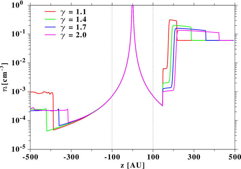
Figure 1.— The number density along the ISM inflow axis in upwind ($z>0$) and downwind ($z<0$) direction in the steady-state configuration of the simulation. The two dotted vertical lines at $z=\pm 100$ AU mark the inner boundary of the computational domain, inside of which the density was estimated according to $\rho\propto r^{-2}$. The first jump in upwind direction is the termination shock, the second one is the heliopause, and the third one is the bow shock. In the downwind direction, there is only a termination shock.

At the inner computational boundary of the model (located at a helio-/astrocentric distance of $r=r_{\rm b}=100$ AU), the upstream temperature $T_{1}$, the thermal pressure $P_{1}$, and the Mach number $M_{1}=v_{1}/c_{1}$ are extrapolated inwards from their respective boundary values using the polytropic relation $P_{1}\propto\rho_{1}^{\gamma}$ and the ideal gas law with

$$P_{1}\propto r^{-2\gamma}\,,\quad T_{1}\propto r^{-2(\gamma-1)}\,,\quad M_{1}\propto r^{\gamma-1}\,.$$ (12)

Moreover, the Mach number at the TS distance can easily be estimated according to formulas (12).

$\gamma$	$c_{\rm s}$ [km/s]	$M$	$M$	$s$
	100 AU	100 AU	150 AU
1.06	19.3	19.1	20.1	33.5	Izmodenov et al.
					(2014)
1.10	16.2	23.2	24.1	20.6	(Fig. 1)
4/3	6.1	61.3	70.2	7.0	electron gas
7/5	4.5	82.7	97.5	5.9	diatomic gases
					(Fig. 1, $\gamma\approx 1.4$)
5/3	1.5	254.2	333.1	4.0	monoatomic gases
					(Fig. 1, $\gamma\approx 1.7$)
2	0.4	1075.5	1613.3	3.0	shallow water waves
					(Fig. 1)

Table 1 The first column shows the polytropic index, the second and third the sound speed and Mach number at 100 AU, and the fourth column the Mach number at the TS at 150 AU. In the fifth column, the corresponding compression ratio is given. Note again the unrealistically high values of $s$ in the first two rows.

The sound speeds and Mach numbers for different polytropic indices are shown in Fig. 2 at 1 AU, 100 AU, and 150 AU (which is the TS distance in upwind direction). From the definition of the sound speed

$$c_{\rm s}:=\sqrt{\frac{\gamma\,kT}{m_{\rm p}}}\,,$$ (13)

where $k$ is the Boltzmann constant, $m_{\rm p}$ the proton mass, and $T$ given by Eq. (12), it follows that $c_{s}|_{1\,{\rm AU}}\propto\sqrt{\gamma}$, while already for slightly larger radii, and particularly for 100 and 150 AU, the $\gamma$ dependence in $T$ dominates, leading to an exponential decay. Consequently, the Mach numbers at 1 AU, 100 AU, and 150 AU show the corresponding inverse behaviors. In Table 1, specific values for sound speed, Mach number, and compression ratio are given for different $\gamma$ values. This table shows that at the TS the hypersonic approximation $M\gg 1$ (see Appendix) can be applied to the Rankine-Hugoniot relations.

Caution has to be taken when choosing the polytropic indices for specific systems: for small $\gamma$’s (i.e., close to unity) the kinetic energy is increasingly transferred into the downstream ram pressure rather than in thermal pressure of the plasma. Moreover, the polytropic index has to be expressed by thermodynamical quantities rather than by the microscopic degrees of freedom, because the latter can become infinitely large and, thus, meaningless for small $\gamma$’s. For a discussion of (multi-)polytropical indices see Livadiotis (2016). Nevertheless, since $\gamma$ in terms of $f$ is from a microphysical point of view more convenient than using a thermodynamical representation, we continue to use $f=2/(\gamma-1)$ and call this “equivalent degrees of freedom”.

As can be seen from Fig. 1, the spatial extent of the IHS along the inflow axis $z$ decreases/increases with decreasing/increasing $\gamma$. Thus, a $\gamma$ smaller than $5/3$ can explain the observed extent of the IHS of roughly 30 AU (Izmodenov et al., 2014). However, simulations including neutrals and magnetic fields are required to estimate the exact behavior. Nevertheless, as discussed by Nicolaou et al. (2014), Jacobs & Poedts (2011), Kartalev et al. (2006), and Farrugia et al. (2001), the polytropic index of the solar wind ranges from 1.4 to 2.1 although it should be noted that these authors neglect the behavior of PUIs; others include temperature anisotropies or $\kappa$ distributions. Including PUIs and following Fahr & Siewert (2015) or Wu et al. (2009), we easily obtain $\gamma>5/3$, leading to an increase of the IHAS’s extent in a hydrodynamic single-fluid model.

For a single-fluid model with a parametric global $\gamma$, the compression ratios change depending on the polytropic index. The standard Rankine-Hugoniot relation defining $s$ gives

$$s=\frac{(\gamma+1)M^{2}_{1}}{(\gamma-1)M^{2}_{1}+2}$$ (14)

(Landau & Lifshitz, 1972). In the limit of infinite Mach numbers, one obtains the maximum compression ratio

$$s_{\textnormal{max}}:=\lim_{M_{1}\rightarrow\infty}s=\frac{\gamma+1}{\gamma-1}\,.$$ (15)

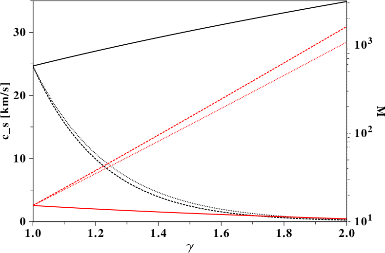
Figure 2.— The sound speeds (black) and Mach numbers (red) as functions of the polytropic index. The left y axis shows the sound speed at 1 AU (solid line), 100 AU (dotted line), and at 150 AU (dashed line). The right y axis shows the logarithm of the Mach number, where the solid, dotted, and dashed lines correspond to the above. For an increasing polytropic index, the sound speed at 1 AU increases, whereas at 100 and 150 AU it decreases. The Mach number shows the opposite behavior.

From Fig. 1, it is also evident that the behaviors in the upwind and tail directions are different: While in the upwind direction the TS remains at the same position, in the tailward direction the TS distance varies with the polytropic index. For $\gamma\neq 4/3$, the TS moves inward. In other words, of all cases shown in Fig. 1, the TS in downwind direction is located farthest from the Sun for $\gamma=4/3$. This maximum is neither theoretically nor empirically determined; it is just the model with the most distant TS in the tail. The difference between the tail and upwind directions is that in the latter, the supersonic solar/stellar wind ram pressure balances that of the ISM, while in the tail direction, it only has to balance the thermal pressure.

In the upwind direction, the TS position is independent of $\gamma$ because the characteristic along the inflow axis is the momentum balance between the total momentum of the ISM and that of the supersonic stellar/solar wind, which in the chosen parameter range is dominated by the ram pressures of both media. Note that the thermal pressure is irrelevant. Thus, the TS distance is (Parker, 1963)

$$r_{\rm TS}=r_{0}\,\frac{v_{\rm sw}}{v_{\rm ism}}\sqrt{\frac{\rho_{\rm sw}}{\rho_{\rm ism}}}$$ (16)

with $r_{0}=1$ AU.

Concluding this section, we state that with different $\gamma$ values the compression ratio and, furthermore, the thickness of the HAS can be changed. Although we have discussed only changes of the IHAS, our results also apply to the OHAS analogously. Deviations of the polytropic index from the mono-atomic $\gamma=5/3$ can be caused, for example, by a mixture of mono-atomic species (like protons) with more complex atoms or by including magnetic fields.

Furthermore, the solar wind polytropic index is expected to change with the solar cycle according to Nicolaou et al. (2014) and Jacobs & Poedts (2011). This will affect the shock structures, but to our knowledge, such a time-dependent model does not yet exist. Nonetheless, a problem with simulating the helio-/astrospheres with globally constant polytropic indices is that the IHAS can shrink but at the cost of an increasing compression ratio, which is not observed for the heliosphere. The idea to avoid this problem is to consider changes of the polytropic index after a shock passage of the solar wind. We discuss this in the following and see that the problem of compression ratios being too large remains.  

4. Variable polytropic indices across a shock

In this section, we discuss the Rankine-Hugoniot relations for the density, pressure, and temperature ratios for systems containing shocks with different upstream and downstream polytropic indices. To this end, we consider the general case of polytropic indices $\gamma_{i}\in\,]1,3]$. Then, for the application to the helio-/astrospheres, we fix the upstream polytropic index to $\gamma_{1}=5/3$.

In the following, only the main results are stated, while technical details are given in the Appendix. Various ratios have already been discussed by Drake (2006) and similarly by Nieuwenhuijzen et al. (1993). The explicit form of the compression ratio given by the latter authors leads, however, in the hypersonic limit of high upstream Mach numbers ($M_{1}\gg 1$) to unexpected results. In this limit, one expects a compression ratio of the form (15) with $\gamma=\gamma_{2}$ (see Eq. (A15) in the Appendix). This is already discussed in Drake (2006), where, however, the various solution branches were not considered. Therefore, we newly perform these calculations following the notation in textbooks like Courant & Friedrichs (1948), Landau & Lifshitz (1972), or Goedbloed et al. (2010).

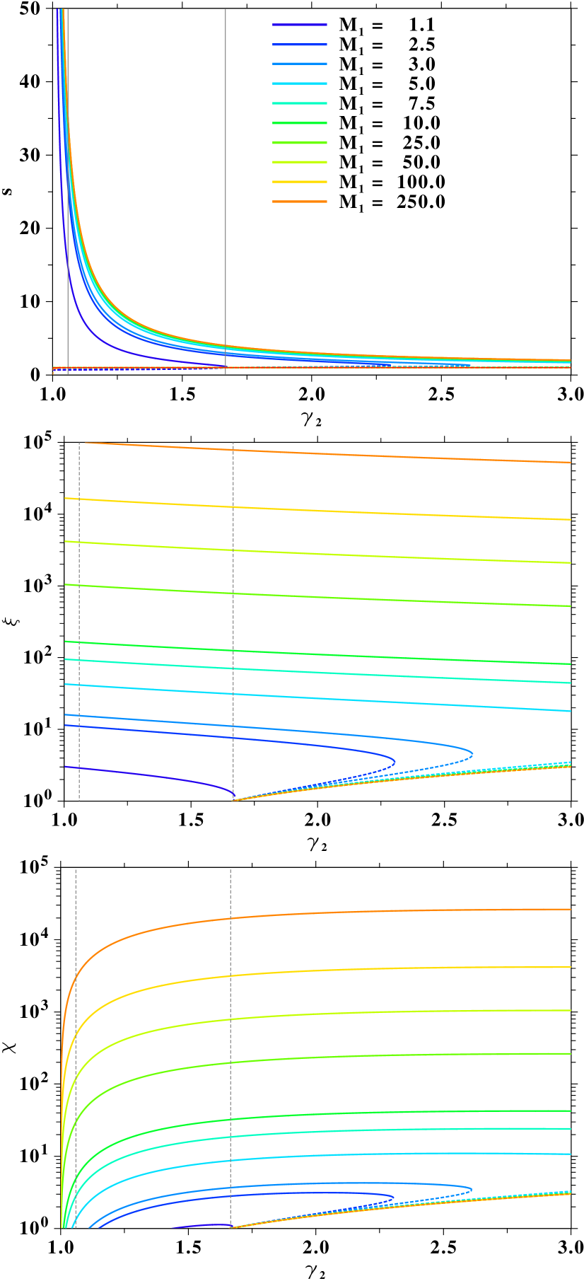
Figure 3.— The ratios $s^{\pm}$ (upper panel, in linear scale), $\xi^{\pm}$ (middle panel, in logarithmic scaling), and $\chi^{\pm}$ (bottom panel, in logarithmic scaling) for a fixed $\gamma_{1}=5/3$ and selected values of $M_{1}$ (as indicated in the legend of the upper panel) as a function of $\gamma_{2}$, with 1 for isothermal conditions (infinite degrees of freedom) and 3 for one degree of freedom. The two vertical lines mark $\gamma_{2}=1.06$ (Izmodenov et al., 2014), and $\gamma_{1}=\gamma_{2}=5/3$. The solid lines correspond to the positive solutions $s^{+},\xi^{+},\chi^{+}$, the dotted lines to the negative ones $s^{-},\xi^{-},\chi^{-}$.

The conservation of energy across a shock is given by

$$w_{1}-w_{2}+\frac{1}{2}(V_{1}+V_{2})(P_{2}-P_{1})=0$$ (17)

with the enthalpies

$$w_{i}=\frac{\gamma_{i}P_{i}V_{i}}{\gamma_{i}-1}$$ (18)

and specific volumes $V_{i}:=1/\rho_{i}$. To include oblique shocks, we use $v_{{\rm n},i}$ to denote the velocity components along the shock normal vector, and the normal Mach number $M_{\rm n,1}:=v_{\rm n,1}/c_{\rm s,1}=M_{1}\sin\vartheta$ with the shock angle $\vartheta$, i.e., the angle between the shock and the inflow velocity. After a short calculation, we find for the compression ratio $s=\rho_{2}/\rho_{1}=v_{\rm n,1}/v_{\rm n,2}$ in the rest frame of the shock

$$s=s^{+}=\frac{M_{\rm n,1}^{2}\gamma_{1}(\gamma_{2}+1)}{(M_{\rm n,1}^{2}\gamma_{1}+1)\gamma_{2}-\Gamma_{12}}\ ,$$ (19)

and for the pressure ratio $\xi=P_{2}/P_{1}$

$$\xi=\xi^{+}=\frac{1}{\gamma_{2}+1}\,\left(M_{\rm n,1}^{2}\gamma_{1}+1+\Gamma_{12}\right)\ ,$$ (20)

where

$$\Gamma_{12}:=\sqrt{\gamma_{1}^{2}M_{\rm n,1}^{4}+\dfrac{2\gamma_{1}M_{\rm n,1}^{2}(\gamma_{1}-\gamma_{2}^{2})}{\gamma_{1}-1}+\gamma_{2}^{2}}\ .$$ (21)

The superscript “$+$” refers to the positive solution branch, as discussed in the Appendix.

Assuming that the temperature obeys the ideal gas law $P_{i}\propto\rho_{i}T_{i}$, we obtain for the temperature ratio $\chi=T_{2}/T_{1}$

$$\chi=\chi^{+}=\frac{P_{2}\,\rho_{1}}{P_{1}\,\rho_{2}}=\frac{\xi^{+}}{s^{+}}\ .$$ (22)

The respective negative branches $s^{-}$, $\xi^{-}$, and $\chi^{-}$ are disregarded for physical reasons; this is discussed in detail in Subsection 5.3.

In the hypersonic limit ($M_{\rm n,1}\gg 1$), the ratios (19), (20), and (22) become

$$s \simeq \frac{\gamma_{2}+1}{\gamma_{2}-1}$$ (23)

$$\xi \simeq \frac{2\gamma_{1}}{\gamma_{2}+1}\,M_{\rm n,1}^{2}$$ (24)

$$\chi \simeq \frac{2\gamma_{1}(\gamma_{2}-1)}{(\gamma_{2}+1)^{2}}\,M_{\rm n,1}^{2}\,.$$ (25)

From Table 1 and the shapes of the functions (19), (20), and (22), one can see that for our simulations the hypersonic approximation is reasonable at the TS. Note that the radicand of $\Gamma_{12}$ in Eq. (21) can become negative for

$$\gamma_{2}<\gamma_{1}\,M_{\rm n,1}\sqrt{\frac{(\gamma_{1}-1)M_{\rm n,1}^{2}+2}{2\gamma_{1}M_{\rm n,1}^{2}-\gamma_{1}+1}}\,\,,$$ (26)

which leads to complex values for the ratios and, thus, non-physical solutions (see Table 2). For $\gamma_{1}=\gamma_{2}$, the above ratios reproduce the well-known results.

$\gamma_{1}$	$\gamma_{2}$	$M_{1}$	$s$	$\xi$	$\chi$	$\zeta$
5/3	1.06	1.001	13.5	2.55	0.19	10.7
5/3	1.06	5.000	31.3	41.34	1.32	71,0
5/3	4/3	1.001	2.5	2.00	0.89	5.9
5/3	4/3	5.000	6.3	36.08	5.7	30.8
4/3	5/3	1.001	— all ratios complex —
4/3	5/3	5.000	3.1	23.65	7.58	0.36

Table 2 The respective ratios of density $s=s(\gamma_{1},\gamma_{2},M_{1})$, pressure $\xi=\xi(\gamma_{1},\gamma_{2},M_{1})$, temperature $\chi=\chi(\gamma_{1},\gamma_{2},M_{1})$, and the ratio of the entropy parameter $\zeta=\zeta(\gamma_{1},\gamma_{2},M_{1})$ (see Eq. (42) below) for specific values of upstream and downstream polytropic indices $(\gamma_{1},\gamma_{2})$ and Mach number $M_{1}$. Allowed solutions are marked by ratios $s$, $\xi$, $\chi$, and $\zeta$ being real and greater than unity.

In Fig. 3, both solutions for the ratios $s^{\pm},\xi^{\pm}$, and $\chi^{\pm}$ are shown. The compression ratio $s^{+}$ increases with decreasing $\gamma_{2}$, which becomes particularly evident in the hypersonic limit (23). The negative solution $s^{-}$ is slightly larger than one for $\gamma_{2}>\gamma_{1}$ and slightly lower one for $\gamma_{2}<\gamma_{1}$. The pressure ratio $\xi^{+}$ grows rapidly with increasing Mach number. For low Mach numbers, it decreases with increasing $\gamma_{2}$ until $\Gamma_{12}$ becomes imaginary. An increase beyond the value determined by Eq. (26) (e.g., $\gamma_{2}<2.02$ for $\gamma_{1}=5/3$ and $M_{1,n}=2$) is not possible. For sufficiently high Mach numbers (i.e., $M_{\rm n,1}>3.6$ for $\gamma_{1}=5/3$ and $\gamma_{2}=3$) all solutions are real in the domain of interest. For constant Mach numbers and given $\gamma_{1}$, the pressure ratio decreases with increasing $\gamma_{2}$. Considering the ratios $s^{+},\xi^{+}$, and $\chi^{+}$, almost all $\gamma_{1}\rightarrow\gamma_{2}$ transitions for high Mach numbers are allowed.

Figure 4.— The entropy ratio $\zeta$ for the positive solutions $\xi^{+}$ and $s^{+}$ (solid lines) and the negative solutions $\xi^{-}$ and $s^{-}$ (dotted lines). The upper panel shows the solution for $\tau=T_{1}/T_{0}=10^{2}$, the middle panel for $\tau=10$, and the lower panel for $\tau=1$. The red horizontal lines indicate the cutoff value $\zeta=1$ (cf. Eq. (43)). The color coding is identical to that of Fig. 3.

Note that also the negative solutions $s^{-},\xi^{-}$, and $\chi^{-}$ can assume real values. Therfore, for given $\gamma_{1}$ and $\gamma_{2}$ a criterion for the selection of the correct solution is required. As shown in the following section, this criterion is provided by the entropy jump condition and the maximum entropy production principle that, to the best of our knowledge, has not been discussed in the literature in this context.  

5. The multi-polytropic entropy difference across a shock

5.1. The absolute entropy for arbitrary degrees of freedom

To determine the entropy difference across a shock, it seems plausible to use the fundamental thermodynamic relation

$${\rm d}\tilde{S}=\frac{k}{2T}{\rm d}(fT)+\frac{p}{T}{\rm d}V$$ (27)

with volume $V$ (not to be confused with the specific volume $V_{i}=1/\rho_{i}$) and a variable degree of freedom $f$. Direct integration of Eq. (27) leads to a non-local expression for the entropy, namely a line-integrated entropy across the shock. Since we are interested in an expression for the entropy that can be evaluated locally, we make use of the absolute entropy $\tilde{S}$ derived by Syrkin (1924) for a gas with arbitrary degrees of freedom given by

$$\tilde{S}=kN\ln\left(\frac{(2\pi m_{0}k)^{f/2}T^{f/2}a_{0}^{(f-3)}Ve^{(1+f/2)}}{Nh^{f}}\right)\,,$$ (28)

where $N$ is the number of particles, $m_{0}$ and $a_{0}$ are the particles’ mass and diameter, $h$ is the Planck constant, and $e=\exp(1)$. Note that the argument of the logarithm is dimensionless.

For later use, we rewrite Eq. (28) in a form with various single logarithms which may carry dimensions. This is guided by the exponents occurring in Eq. (28). Further, we define the dimensionless entropy per particle $S:=\tilde{S}/(kN)$, which can be expressed as

$$S = \frac{f}{2}\left[\ln T+\ln\left(\frac{2\pi ekm_{0}a_{0}^{2}}{h^{2}}\right)\right]$$

$$-\left[\ln(n)+\ln\left(\frac{a_{0}^{3}}{e}\right)\right]$$

using $n=N/V$. The constant

$$\frac{2\pi ek\,m_{0}a_{0}^{2}}{h^{2}}=:\frac{1}{T_{0}}\ ,$$ (30)

i.e., the argument of the second logarithm, has the dimension of an inverse temperature $T_{0}$, and, thus, cancels the dimension of the argument in the first term. Likewise,

$$\frac{a_{0}^{3}}{e}=:\frac{1}{n_{0}}$$ (31)

has dimension of a volume (or inverse number density), and cancels the dimension of $\ln(n)$. The absolute entropy (5.1) now assumes the rather compact form

$$S = \frac{f}{2}\ln\left(\frac{T}{T_{0}}\right)-\ln\left(\frac{n}{n_{0}}\right)\ .$$ (32)

In the next step, the constants $T_{0}$ and $n_{0}$, which depend on the particle mass $m_{0}$ and diameter $a_{0}$ are fixed. While the proton mass $m_{\rm p}$ is easily identified as a suitable choice for $m_{0}$, it would not be appropriate in this context to use the proton “diameter” $a_{\rm p}$ for $a_{0}$ for the following reason: In Syrkin’s derivation of formula (28), the particle diameter appears as a measure of the minimum distance between adjacent particles. But in a plasma, it is from a physical point of view not possible to place two protons directly side by side. Choosing the hydrogen atom diameter is, thus, more appropriate because a plasma is always quasi-neutral. Since a plasma at low temperatures tends to recombine and neutralize, we, however, consider a somewhat larger diameter given by the classical Bohr radius, which enables the plasma to stay in its quasi-neutral state, i.e., a mixture of protons and electrons (and not a (hydrogen) gas). Therefore, with the Bohr radius of the hydrogen atom $r_{\rm B}=5.291\times 10^{-9}$ cm, we obtain after normalizing Eqs. (30) and (31) to $m_{0}=m_{\rm p}$ and $a_{0}=a_{\rm B}=2r_{\rm B}$,

$$T_{0} = (99.5\ {\rm K})\left(\frac{m_{0}}{m_{\rm p}}\right)^{-2}\left(\frac{a_{0}}{a_{\rm B}}\right)^{-1}$$ (33)

$$n_{0} = (2.3\times 10^{24}\ {\rm cm}^{-3})\left(\frac{a_{0}}{a_{\rm B}}\right)^{-3}\ .$$ (34)

In the following, we approximate $T_{0}\approx 100$ K.

As an example, we compute the total entropy of a dense H₂ molecular cloud with $T=100$ K and $n=100$ cm^-3 assuming that at this temperature all degrees of freedom except those of translational motion are frozen-in (implying $f=3$). We approximate the radius and mass of the H₂ molecule by twice the values for a single hydrogen atom. We obtain an absolute normalized entropy per particle of $S\approx 53$. Note that the absolute entropy per particle (32) is dominated by the normalization density $n_{0}$ for a wide range of astrophysical applications, for example, ISM or astrospherical shocks, because the temperature is usually below $T<10^{9}$ K. For other scenarios, like stellar cores, the density $n$ can easily become larger than $n_{0}$.  

5.2. Entropy difference for arbitrary degrees of freedom

We now consider variable degrees of freedom through a shock passage and calculate the entropy difference as the difference of the absolute entropies (32) from each side.

The conservation law for the specific entropy with the fluid velocity $\vec{v}$ reads

$$\frac{\partial(\rho S)}{\partial t}+\nabla\cdot(\rho\vec{v}S)=0\,.$$ (35)

Because a shock is an irreversible transition, the corresponding Rankine-Hugoniot condition (Goedbloed et al., 2010) is

$$-u[S_{1}-S_{2}]+\rho_{1}v_{\rm n,1}S_{1}-\rho_{2}v_{\rm n,2}S_{2}\leq 0\,,$$ (36)

where $u$ is the shock speed and $v_{\rm n}$ its component normal to the shock. Using the equation of continuity $\rho_{1}v_{\rm n,1}=\rho_{2}v_{\rm n,2}$, this leads for a stationary shock ($u=0$) to

$$S_{2}-S_{1}\geq 0\,.$$ (37)

Allowing for different degrees of freedom before and after the shock, we can compute the normalized entropy difference up- and downstream of a shock by means of Eq. (32). We find

$$S_{2}-S_{1} = \frac{f_{2}}{2}\ln\left(\frac{T_{2}}{T_{1}}\right)-\ln\left(\frac{n_{2}}{n_{1}}\right)$$

$$+\frac{f_{2}-f_{1}}{2}\ln\left(\frac{T_{1}}{T_{0}}\right)\geq 0\,.$$

Keeping in mind that for some applications like astrospherical shocks we may also encounter different (e.g., dissociative) species on both sides of the shock, we need to use different values for $(m_{0},a_{0})$, and, therefore, different values for $(T_{0},n_{0})$. In this case, the following term has to be added to the right-hand side of Eq. (5.2)

$$-\frac{f_{2}}{2}\ln\left(\frac{T_{0,2}}{T_{0,1}}\right)+\ln\left(\frac{n_{0,2}}{n_{0,1}}\right)$$ (39)

$$= \frac{f_{2}}{2}\ln\left(\frac{m_{0,2}}{m_{0,1}}\right)+\left(f_{2}-3\right)\,\ln\left(\frac{a_{0,2}}{a_{0,1}}\right)\,.$$

Then, however, we cannot use only the difference of the normalized entropies (5.2), but have also to take into account different numbers of particles $N_{1}\neq N_{2}$ and additional mixing terms. For our application, we assume that we have the same kind of particles on both sides of the shock.

Requiring the validity of the ideal gas law on both sides of the shock, formula (5.2) can easily be reformulated in terms of the ratios $\chi$ and $s$ as

$$S_{2}-S_{1} = \frac{f_{2}}{2}\ln(\chi)-\ln(s)+\frac{f_{2}-f_{1}}{2}\ln\left(\frac{T_{1}}{T_{0}}\right)\geq 0\,.\quad\quad$$ (40)

We remark that both ratios are functions of the upstream parameters $M_{1}$ and $f_{1}$ as well as the downstream degree of freedom $f_{2}$, which is assumed to be independent of the upstream values. However, for the excitations of higher degrees of freedom, e.g., by rotations or vibrations, the downstream temperature needs to be high and, thus, $f_{2}$ will depend on the underlying physical process.

In terms of the pressure ratio $\xi$ and the polytropic indices $\gamma_{1},\gamma_{2}$, the inequality (40) reads

$$\frac{\ln(\xi)-\gamma_{2}\ln(s)}{\gamma_{2}-1}+\frac{\gamma_{1}-\gamma_{2}}{(\gamma_{1}-1)(\gamma_{2}-1)}\ln\left(\frac{T_{1}}{T_{0}}\right)\geq 0$$ (41)

using the definition of the equivalent degrees of freedom $f_{i}=2/(\gamma_{i}-1)$. In order to obtain the ratio

$$\zeta:=\left(\exp(S_{2})/\exp(S_{1})\right)^{\gamma_{2}-1}\ ,$$ (42)

we take the exponential of (41) and get

$$\zeta=\xi\,s^{-\gamma_{2}}\left(\frac{T_{1}}{T_{0}}\right)^{\frac{\gamma_{1}-\gamma_{2}}{\gamma_{1}-1}}\geq 1\,.$$ (43)

In terms of the degrees of freedom and the temperature ratio, this relation yields

$$\chi^{f_{2}}s^{-2}\left(\frac{T_{1}}{T_{0}}\right)^{f_{2}-f_{1}}\geq 1\,.$$ (44)

Note that the right hand side differs from unity only if degrees of freedom change across the shock.

In Fig. 4, the ratio $\zeta$ as function of $\gamma_{2}$ for a fixed $\gamma_{1}$ is shown for three different values of the ratio $\tau:=T_{1}/T_{0}$, namely $\tau=100$, $\tau=10$, and $\tau=1$. For $\tau=10,100$, the entropy ratio first increases rapidly for all displayed Mach numbers, and after reaching a maximum, it decreases to values below unity for $M<250$. The increase of the entropy ratio for $\tau=1$ is also quite fast for small values of $\gamma_{2}$. For larger values of $\gamma_{2}$ the entropy ratio becomes approxmately constant until it finally slowly decreases. This is the limiting case for physical solutions because then the plasma freezes out and we obtain recombined neutral atoms. We point out that in (44) the case $\tau=1$ is not identical to the case where $\gamma_{1}=\gamma_{2}$ because $s$ and $\chi$ depend both on $\gamma_{1}$ and $\gamma_{2}$. Moreover, for all $tau$’s the entropy ratios resulting from the negative roots $\xi^{-}$ and $s^{-}$ are also allowed because they can be larger than unity.

5.3. Discussion of the negative roots

The solutions for the compression and pressure ratios (and, thus, the temperature and entropy ratios) consist each of two branches $s^{\pm}$, $\xi^{\pm}$, which depend on the sign in front of $\Gamma_{12}$ (see Eq.(A.1)).

The positive solutions represent the standard compression shocks, whereas the negative solutions are rarefaction shocks as discussed in the literature for special “fluids”, i.e., so-called BZT fluids (Bethe-Zeldovitch-Thompson); for details see Cramer & Park (1999). Here, the rarefaction shocks must be excluded because of the maximum entropy production principle (Martyushev, 2013): In all cases where both solutions are allowed simultaneously, the entropy production for the positive solutions is always larger as for the negative roots (cf. Fig. 4).  

5.4. Application to the helio-/astrospheres

In our studies of the helio- and astrospheres, variable polytropic indices have been used. We have calculated for specific values of $\gamma_{1}$, $\gamma_{2}$, and $M_{1}$ the compression, pressure, and temperature ratios as well as the entropy difference (see Table 2). Some ratios become complex-valued, which is caused by a negative radicand of the square root (21) and, thus, not all values of $\gamma_{1},\gamma_{2}$, in addition to the cases where $\zeta<1$, lead to physical solutions. Therefore, variable polytropic indices across a (termination) shock can easily lead to unrealistic physical conditions. This is particularly true for large-scale helio-/astrospherical simulations, where in the flank regions the Mach numbers can become small.  

6. Discussion and conclusions

In this work, we have derived multi-polytropic generalized Rankine-Hugoniot relations. We gave explicit expressions for the ratios of the densities, pressures, and temperatures across a shock. The derivation included, for the first time, a consistent consideration of the associated change in entropy.

For the examples of the helio-/astrospheres, we have discussed, on the one hand, the case of different globally constant polytropic indices and, on the other hand, a changing polytropic index in a shock transition. The polytropic index in the solar wind is varying and usually different from $5/3$. For smaller values of $\gamma$ in the entire integration region (also in the ISM), the thickness of the IHAS and OHAS in upwind direction shrinks, while for higher values, it grows. In the former case, the compression ratio increases, while in the latter it decreases. A decrease in the compression ratio is needed in order to explain the Voyager observations, while an increase for small $\gamma$’s is incompatible with the observations.

Since the compression ratio, which is an important quantity for the acceleration of particles, is a function of the polytropic index, it is of great interest to study astrospheres under varying polytropic indices in order to analyze the acceleration of energetic particles.

The interaction of astrospheres, whose abundances are not solar-like, with the ISM can lead to a change in the polytropic index beyond the (bow) shock passage. This is particularly true when a star is born in a cold H₂ cloud, where the diatomic hydrogen dissociates after the shock passage. Relation (40) can be adapted to this case, taking into account the different numbers of particles $N_{1}$, $N_{2}$, and possible mixing terms, however, it will require a multi-fluid description of the shock transition region.

Thus, a detailed study of multi-fluid models with different polytropic indices not only across the shock, but for example also for different species like for solar/stellar wind protons and PUIs is needed. The problem at the moment is that to our knowledge the available simulation codes cannot yet handle such a setting. Further, it is not clear if such a configuration is at all thermodynamically possible for fluids (see McKee & Holliman (1999) for multi-pressure polytropes to model the structure and stability of molecular clouds).

We point out that the above study is not restricted to the applications of helio- and astrospheres but concerns all scenarios in which the polytropic index varies over a hydrodynamic shock, e.g., interstellar shocks (for example Pittard & Parkin, 2016) or supernova explosions (for example Bolte et al., 2015).

For MHD shocks, the situation is more complicated because the jump conditions are characterized by a three-parameter family (the normal alfvénic Mach number, the ratio between the thermal and magnetic field pressure, and the angle between the inflow and magnetic field vector), whereas for hydrodynamical shocks, they are characterized by a one-parameter family (the normal Mach number). The more challenging task of MHD shocks with varying polytropic indices will be addressed in a future study.

Appendix A Generalized mulit-polytropic Rankine-Hugoniot relations

A.1. The pressure ratio $\xi$

Substituting the enthalpy (18) into the equation of energy conservation (17) gives

$$\frac{\gamma_{1}P_{1}V_{1}}{\gamma_{1}-1}-\frac{\gamma_{2}P_{2}V_{2}}{\gamma_{2}-1}+\frac{1}{2}(V_{1}+V_{2})(P_{2}-P_{1})=0\,.$$ (A1)

From this, it immediately follows that

$$\frac{V_{1}}{V_{2}}=\frac{(\gamma_{2}-1)P_{1}+(\gamma_{2}+1)P_{2}}{(\gamma_{1}+1)P_{1}+(\gamma_{1}-1)P_{2}}\times\frac{\gamma_{1}-1}{\gamma_{2}-1}\,.$$ (A2)

Furthermore, using Eq. (A2) and the pressure ratio $\xi=P_{2}/P_{1}$, the square of the mass current $j$ becomes

$$j^{2} = \frac{P_{2}-P_{1}}{V_{1}-V_{2}}=\dfrac{P_{1}}{2V_{1}}(\xi-1)\,\frac{\left[\gamma_{2}-1+(\gamma_{2}+1)\xi\right]\left[\gamma_{1}-1\right]}{-\gamma_{2}+1+(\gamma_{1}-1)\xi}\,.$$ (A3)

With the velocities $v_{i}=jV_{i}$ and the Mach numbers $M_{i}=v_{i}/c_{\rm s,i}$, we obtain from Eq. (A3) and the defining relation for the upstream sound speed

$$c_{\rm s,i}=\sqrt{\gamma_{i}P_{i}V_{i}}$$ (A4)

after some algebraic manipulations

$$\frac{2M_{1}^{2}\,\gamma_{1}}{\gamma_{1}-1} = (1-\xi)\,\frac{\gamma_{2}-1+(\gamma_{2}+1)\xi}{\gamma_{2}-1-(\gamma_{1}-1)\xi}$$

$$\Leftrightarrow\,\xi^{\pm} = \frac{1}{\gamma_{2}+1}\,\bigl{(}M_{1}^{2}\gamma_{1}+1\pm\Gamma_{12}\bigr{)}\,,$$ (A5)

where the superscripts $\pm$ denote the two roots and

$$\Gamma_{12}:=\sqrt{\gamma_{1}^{2}M_{1}^{4}+2\gamma_{1}M_{1}^{2}\,\frac{\gamma_{1}-\gamma_{2}^{2}}{\gamma_{1}-1}+\gamma_{2}^{2}}\,.$$ (A6)

Setting $\gamma_{1}=\gamma_{2}=\gamma$ yields

$$\left(\xi^{+},\xi^{-}\right)=\left(\frac{2\gamma M_{1}^{2}-\gamma+1}{\gamma+1}\,,1\right)\,,$$ (A7)

which is the usual Rankine-Hugoniot relation for $\xi^{+}$ and that for rarefaction shocks for $\xi^{-}$ (see Section 5.3).  

A.2. The compression ratio

Rewriting Eq. (A3), we obtain for the square of the mass current

$$j^{2}=\frac{P_{1}(\xi-1)s}{V_{1}(s-1)}\,,$$ (A8)

where $s=V_{1}/V_{2}$ is the compression ratio. On the other hand, using the expressions for $v_{1}$, $M_{1}$, and $c_{\rm s,1}$, we find

$$j^{2}=\frac{M_{1}^{2}\gamma_{1}P_{1}}{V_{1}}\,.$$ (A9)

Combining Eqs. (A8) and (A9) leads after some algebra to

$$s=\frac{M_{1}^{2}\gamma_{1}}{M_{1}^{2}\gamma_{1}+1-\xi}\,.$$ (A10)

Substituting the solutions (A5) for the pressure ratio, we find

$$s^{\pm}=\frac{M_{1}^{2}\gamma_{1}(\gamma_{2}+1)}{(M_{1}^{2}\gamma_{1}+1)\gamma_{2}\mp\Gamma_{12}}\,.$$ (A11)

In the case $\gamma_{1}=\gamma_{2}=\gamma$, these simplify to

$$\left(s^{+},s^{-}\right)=\left(\frac{(\gamma+1)M_{1}^{2}}{(\gamma-1)M_{1}^{2}+2},1\right)\,,$$ (A12)

where the solution $s^{+}$ is again the standard Rankine-Hugoniot compression ratio.  

A.3. The temperature ratio $\chi$

The temperature ratio $\chi$ is given by

$$\chi = \frac{T_{2}}{T_{1}}=\frac{P_{2}}{P_{1}}\frac{\rho_{1}}{\rho_{2}}=\frac{\xi}{s}\ ,$$ (A13)

which can be easily calculated in terms of Eqs. (A.1) and (A11).  

A.4. The shocked Mach number

From Eq. (17), the shocked Mach number $M_{2}$ becomes

$$M_{2}^{2}=\frac{1}{\gamma_{2}}\frac{\gamma_{1}M_{1}^{2}}{s+\gamma_{1}M_{1}^{2}(s-1)}\,.$$ (A14)

A.5. Hypersonic limits

The hypersonic limits of the pressure, compression, and temperature ratios as well as that of the shocked Mach number are computed by considering large upstream Mach numbers $M_{1}\gg 1$ in Eqs. (A.1), (A11), and (A13) for the relevant values of $\gamma_{1},\gamma_{2}$, resulting in the expressions

$$\left(\xi^{+},\xi^{-}\right) \simeq \left(\frac{2\gamma_{1}}{\gamma_{2}+1}M_{1}^{2}\,,\ \frac{\gamma_{2}-1}{\gamma_{1}-1}\right)$$ (A15)

$$\left(s^{+},s^{-}\right) \simeq \left(\frac{\gamma_{2}+1}{\gamma_{2}-1}\,,1\right)$$ (A16)

$$\left(\chi^{+},\chi^{-}\right) \simeq \left(\frac{2\gamma_{1}(\gamma_{2}-1)}{(\gamma_{2}+1)^{2}}M_{1}^{2}\,,\ \frac{\gamma_{2}-1}{\gamma_{1}-1}\right)$$ (A17)

$$\left(M_{2}^{+},M_{2}^{-}\right) \simeq \left(\sqrt{\frac{\gamma_{2}-1}{2\gamma_{2}}}\,,\ \sqrt{\frac{\gamma_{1}}{\gamma_{2}}}M_{1}\right)\,.$$ (A18)

Note that the compression ratio $s^{+}$ is independent of $\gamma_{1}$. Moreover, in the case $\gamma_{1}=\gamma_{2}$, the standard Rankine-Hugoniot relations for high Mach numbers (positive roots) are recovered.

A.6. Oblique shocks

Replacing the Mach number $M_{1}$ by $M_{1}\sin\vartheta$ and $v_{i}$ by $v_{{\rm n},i}=\vec{n}\cdot\vec{v}_{i}$, also oblique shocks can be studied. Here, $\vec{n}$ is the shock normal vector and $\vartheta$ the angle between the shock and the inflow velocity.

References

- Arthur (2007) Arthur, S. 2007, Rev. Mex. Astron. Astrophys., 30, 64
- Bolte et al. (2015) Bolte, J., Sasaki, M., & Breitschwerdt, D. 2015, A&A, 582, A47
- Borrmann & Fichtner (2005) Borrmann, T., & Fichtner, H. 2005, Adv. Space Res., 35, 2091
- Buitrago & Calvo-Mozo (2010) Buitrago, J. C., & Calvo-Mozo, B. 2010, Rev. Colomb. Fis., 42, 1
- Chandrasekhar (1939) Chandrasekhar, S. 1939, An introduction to the study of stellar structure (Chicago, Ill., The University of Chicago press [1939])
- Chashei et al. (2003) Chashei, I. V., Fahr, H. J., & Lay, G. 2003, Advances in Space Research, 32, 507
- Courant & Friedrichs (1948) Courant, R., & Friedrichs, K. O. 1948, Supersonic flow and shock waves (New York: Interscience)
- Cramer & Park (1999) Cramer, M. S., & Park, S. 1999, Journal of Fluid Mechanics, 393, 1
- Drake (2006) Drake, R. P. 2006, High-Energy-Density Physics: Fundamentals, Inertial Fusion, and Experimental Astrophysics (Springer)
- Eddington (1938) Eddington, Sir, A. S. 1938, MNRAS, 99, 4
- Emden (1907) Emden, R. 1907, Gaskugeln (Leipzig, Verlag B.G. Teubner)
- Fahr (2002a) Fahr, H. J. 2002a, Sol. Phys., 208, 335
- Fahr (2002b) —. 2002b, Annales Geophysicae, 20, 1509
- Fahr et al. (1977) Fahr, H. J., Bird, M. K., & Ripken, H. W. 1977, A&A, 58, 339
- Fahr & Chalov (2008) Fahr, H. J., & Chalov, S. V. 2008, A&A, 490, L35
- Fahr et al. (2000) Fahr, H. J., Kausch, T., & Scherer, H. 2000, A&A, 357, 268
- Fahr & Rucinski (2002) Fahr, H. J., & Rucinski, D. 2002, Nonlinear Processes in Geophysics, 9, 377
- Fahr & Siewert (2013) Fahr, H.-J., & Siewert, M. 2013, A&A, 558, A41
- Fahr & Siewert (2015) —. 2015, A&A, 576, doi:10.1051/0004-6361/201424485
- Farrugia et al. (2001) Farrugia, C. J., Erkaev, N. V., Vogl, D. F., et al. 2001, J. Geophys. Res., 106, 29373
- Goedbloed et al. (2010) Goedbloed, J. P., Keppens, R., & Poedts, S. 2010, Advanced Magnetohydrodynamics (Cambridge, UK: Cambridge University Press)
- Horedt (2004) Horedt, G. P., ed. 2004, Astrophysics and Space Science Library, Vol. 306, Polytropes - Applications in Astrophysics and Related Fields
- Izmodenov et al. (2014) Izmodenov, V. V., Alexashov, D. B., & Ruderman, M. S. 2014, ApJ, 795, L7
- Jacobs & Poedts (2011) Jacobs, C., & Poedts, S. 2011, Advances in Space Research, 48, 1958
- Kartalev et al. (2006) Kartalev, M., Dryer, M., Grigorov, K., & Stoimenova, E. 2006, Journal of Geophysical Research (Space Physics), 111, 10107
- Keppens & Goedbloed (1999) Keppens, R., & Goedbloed, J. P. 1999, A&A, 343, 251
- Kissmann et al. (2008) Kissmann, R., Kleimann, J., Fichtner, H., & Grauer, R. 2008, MNRAS, 391, 1577
- Kleimann et al. (2009) Kleimann, J., Kopp, A., Fichtner, H., & Grauer, R. 2009, Annales Geophysicae, 27, 989
- Landau & Lifshitz (1972) Landau, L. D., & Lifshitz, E. M. 1972, Hydrodynamik (Berlin: Akademie-Verlag)
- Livadiotis (2015) Livadiotis, G. 2015, ApJ, 809, 111
- Livadiotis (2016) —. 2016, ApJS, 223, 13
- Livadiotis & McComas (2013) Livadiotis, G., & McComas, D. J. 2013, Space Sci. Rev., 175, 183
- Martyushev (2013) Martyushev, L. 2013, Entropy, 15, 1152
- McKee & Holliman (1999) McKee, C. F., & Holliman, II, J. H. 1999, ApJ, 522, 313
- Moran et al. (2014) Moran, M. J., Shapiro, H. N., & Boettner, D. D. 2014, Fundamentals of Engineering Thermodynamics (Wiley)
- Müller et al. (2008) Müller, H.-R., Florinski, V., Heerikhuisen, J., et al. 2008, A&A, 491, 43
- Nicolaou et al. (2014) Nicolaou, G., Livadiotis, G., & Moussas, X. 2014, Sol. Phys., 289, 1371
- Nieuwenhuijzen et al. (1993) Nieuwenhuijzen, H., de Jager, C., Cuntz, M., Lobel, A., & Achmad, L. 1993, A&A, 280, 195
- Oliveira (2013) Oliveira, M. J. d. 2013, Equilibrium Theromdynamics (Springer Heidelberg New York Dordrecht London), doi:10.1007/978-3-642-36549-2
- Parker (1958) Parker, E. N. 1958, ApJ, 128, 664
- Parker (1963) —. 1963, Interplanetary dynamical processes. (New York, Interscience Publishers, 1963.)
- Pauls & Zank (1996) Pauls, H. L., & Zank, G. P. 1996, J. Geophys. Res., 101, 17081
- Pittard & Parkin (2016) Pittard, J. M., & Parkin, E. R. 2016, MNRAS, 457, 4470
- Pomoell & Vainio (2012) Pomoell, J., & Vainio, R. 2012, ApJ, 745, 151
- Pomoell et al. (2011) Pomoell, J., Vainio, R., & Kissmann, R. 2011, Astrophysics and Space Sciences Transactions, 7, 387
- Richardson et al. (2008) Richardson, J. D., Kasper, J. C., Wang, C., Belcher, J. W., & Lazarus, A. J. 2008, Nature, 454, 63
- Roussev et al. (2003) Roussev, I. I., Gombosi, T. I., Sokolov, I. V., et al. 2003, ApJ, 595, L57
- Sackur (1913) Sackur, O. 1913, Annalen der Physik, 345, 87
- Scherer et al. (2016) Scherer, K., Fichtner, H., Kleimann, J., et al. 2016, A&A, 586, A111
- Scherer et al. (2015) Scherer, K., van der Schyff, A., Bomans, D. J., et al. 2015, A&A, 576, A97
- Siewert & Fahr (2007) Siewert, M., & Fahr, H.-J. 2007, A&A, 471, 7
- Siewert & Fahr (2008) —. 2008, A&A, 485, 327
- Syrkin (1924) Syrkin, J. K. 1924, Zeitschrift fur Physik, 24, 355
- Totten et al. (1996) Totten, T. L., Freeman, J. W., & Arya, S. 1996, J. Geophys. Res., 101, 15629
- Wiengarten et al. (2015) Wiengarten, T., Fichtner, H., Kleimann, J., & Kissmann, R. 2015, ApJ, 805, 155
- Wu et al. (2009) Wu, P., Winske, D., Gary, S. P., Schwadron, N. A., & Lee, M. A. 2009, Journal of Geophysical Research (Space Physics), 114, 8103
- Zeuner (1887) Zeuner, G. 1887, Technische Thermodynamik (Leipzig, Verlag Arthur Felix)