Simplified P_N Equations for Nonclassical Transport with Isotropic Scattering

Abstract

An asymptotic analysis is used to derive a set of diffusion approximations to the nonclassical transport equation with isotropic scattering. These approximations are shown to reduce to the simplified P_N equations under the assumption of classical transport, and therefore are labeled nonclassical SP_N equations. In addition, the nonclassical SP_N equations can be manipulated into a classical form with modified parameters, which can be implemented in existing SP_N codes. Numerical results are presented for an one-dimensional random periodic system, validating the theoretical predictions.

I Introduction

The nonclassical theory of linear particle transport [1, 2] was developed to address transport problems in which the particle flux is not attenuated exponentially. This is the case in certain inhomogeneous random media in which the locations of the scattering centers are spatially correlated. The nonclassical transport equation consists of a linear Boltzmann equation on an extended phase space, able to model particle transport for any given free-path distribution. Applications of this nonclassical theory include neutron transport in reactor cores (cf. [3]), radiative transfer in atmospheric clouds (cf. [4]), and computer graphics (cf. [5]).

In this paper we consider the one-speed nonclassical transport equation with isotropic scattering. This equation is written as

$$\frac{\partial\Psi}{\partial s}(s)+{\bf\Omega}\cdot{\bf\nabla}\Psi(s)+\Sigma_{t}(s)\Psi(s)=\frac{\delta(s)}{4\pi}\left[\int_{4\pi}\int_{0}^{\infty}c\Sigma_{t}(s^{\prime})\Psi({\bm{x}},{\bf\Omega}^{\prime},s^{\prime})ds^{\prime}d\Omega^{\prime}+Q({\bm{x}})\right],$$ (1)

where $s$ describes the free-path of a particle (distance traveled since the particle’s previous interaction), $\Psi(s)=\Psi({\bm{x}},{\bf\Omega},s)$ is the nonclassical angular flux, $c$ is the scattering ratio (probability of scattering), and $Q$ is an isotropic source. The total cross section $\Sigma_{t}$ is a function of the free-path $s$ and satisfies

$$p(s)=\Sigma_{t}(s)e^{-\int_{0}^{s}\Sigma_{t}(s^{\prime})ds^{\prime}},$$ (2)

where $p(s)$ is the free-path distribution function.

The particle flux in its standard definition can be recovered from the solution of Eq. 1 by integrating over the free-path $s$, such that

$$\Psi_{c}({\bm{x}},{\bf\Omega})=\int_{0}^{\infty}\Psi({\bm{x}},{\bf\Omega},s)ds=\text{classical angular flux,}$$ (3a)

and

$$\Phi({\bm{x}})=\int_{4\pi}\int_{0}^{\infty}\Psi({\bm{x}},{\bf\Omega},s)dsd\Omega=\text{scalar flux}.$$ (3b)

For $m=0,1,2,...,$ we define the $m$-th raw moment of $p(s)$ as

$$\big{<}s^{m}\big{>}=\int_{0}^{\infty}s^{m}p(s)ds.$$ (4a)

The following identity holds for $$m=1,2,...$$ :

$$\big{<}s^{m}\big{>}=m\int_{0}^{\infty}s^{m-1}e^{-\int_{0}^{s}\Sigma_{t}(s^{\prime})ds^{\prime}}ds.$$ (4b)

Assuming $\big{<}s^{2}\big{>}<\infty$, an asymptotic approximation of Eq. 1 for the scalar flux given in Eq. 3b has been formally derived [1, 2]:

$$-\frac{1}{6}\frac{\big{<}s^{2}\big{>}}{\big{<}s\big{>}}\nabla^{2}\Phi({\bm{x}})+\frac{1-c}{\big{<}s\big{>}}\Phi({\bm{x}})=Q({\bm{x}}).$$ (5)

Convergence of Eq. 1 to the nonclassical diffusion equation (Eq. 5) has been rigorously discussed in [6].

If the free-path distribution is given by the exponential $p(s)=\Sigma_{t}e^{-\Sigma_{t}s}$, the raw moments defined in Eq. 4 yield

$$\big{<}s^{m}\big{>}=\int_{0}^{\infty}s^{m}\Sigma_{t}e^{-\Sigma_{t}s}ds=\frac{m!}{\Sigma_{t}^{m}}.$$ (6)

In this situation, Eq. 1 reduces to the classical transport equation

$${\bf\Omega}\cdot{\bf\nabla}\Psi_{c}({\bm{x}},{\bf\Omega})+\Sigma_{t}\Psi_{c}({\bm{x}},{\bf\Omega})=\frac{1}{4\pi}\left[c\Sigma_{t}\Phi({\bm{x}})+Q({\bm{x}})\right],$$ (7a)

and Eq. 5 reduces to

$$-\frac{1}{3\Sigma_{t}}\nabla^{2}\Phi({\bm{x}})+\Sigma_{a}\Phi({\bm{x}})=Q({\bm{x}}),$$ (7b)

where $\Sigma_{a}=(1-c)\Sigma_{t}$ is the absorption cross section.

The classical diffusion equation (7b) has been generalized to the hierarchy of the simplified P_N (SP_N) equations, first derived by Gelbard [7, 8, 9]. These equations were shown to be a high-order asymptotic approximation of the transport equation [10]. We refer the reader to [11] for a complete review on SP_N theory.

In this paper we use an asymptotic analysis to derive more accurate diffusion approximations to Eq. 1. We show that, if $p(s)$ is given by an exponential (classical transport), these approximations reduce to the classical SP_N equations; therefore, they are labeled nonclassical SP_N equations.

The remainder of this paper is organized as follows. The asymptotic analysis is carried out in Section II, in which we also provide explicit formulations for the nonclassical SP₁ (diffusion), SP₂, and SP₃ equations. Nonclassical SP_N equations for $N>3$ can be derived by continuing the same procedure. In Section III we show that if Eq. 6 holds (classical transport), the nonclassical SP_N equations reduce to the classical SP_N equations. In Section IV we show that the nonclassical SP_N equations can be manipulated into a classical form with modified parameters, allowing the use of classical Marshak boundary conditions. Section V describes numerical results that validate the theoretical predictions. We conclude with a brief discussion in Section VI.

II Asymptotic Analysis

Let us write Eq. 1 in the mathematically equivalent form

$$\frac{\partial\Psi}{\partial s}(s)+{\bf\Omega}\cdot{\bf\nabla}\Psi(s)+\Sigma_{t}(s)\Psi(s)=0,\qquad s>0,$$ (8a)

$$\Psi(0)=\frac{1}{4\pi}\left[\int_{4\pi}\int_{0}^{\infty}c\Sigma_{t}(s^{\prime})\Psi({\bm{x}},{\bf\Omega}^{\prime},s^{\prime})ds^{\prime}d\Omega^{\prime}+Q({\bm{x}})\right],$$ (8b)

where $\Psi(0)=\displaystyle{\lim_{s\to 0^{+}}\Psi(s)}=\Psi(0^{+})$. Defining $0<\varepsilon\ll 1$, we perform the following scaling:

$$\Sigma_{t}(s) =\frac{\Sigma_{t}(s/\varepsilon)}{\varepsilon},$$ (9a)

$$c =1-\varepsilon^{2}\kappa,$$ (9b)

$$Q({\bm{x}}) =\varepsilon q({\bm{x}}),$$ (9c)

where $$\kappa q O(1) \big{<}s^{m}\big{>}_{\varepsilon}$$ and are . Equations 9a, 9b and 9c are equivalent to the scaling used in [10] to obtain the classical SP_N approximations for Eq. 7a. Moreover, using Eqs. 2, 4a and 9a, we can define such that

$$\big{<}s^{m}\big{>} =\varepsilon^{m}\int_{0}^{\infty}\left(\frac{s}{\varepsilon}\right)^{m}\frac{1}{\varepsilon}\Sigma_{t}(s/\varepsilon)e^{-\int_{0}^{s}\frac{1}{\varepsilon}\Sigma_{t}(s^{\prime}/\varepsilon)ds^{\prime}}ds$$ (9d)

$$=\varepsilon^{m}\int_{0}^{\infty}s^{m}\Sigma_{t}(s)e^{-\int_{0}^{s}\Sigma_{t}(s^{\prime})ds^{\prime}}ds$$

$$=\varepsilon^{m}\big{<}s^{m}\big{>}_{\varepsilon},$$

where $\big{<}s^{m}\big{>}_{\varepsilon}$ is $O(1)$. This scaling implies that:

• The system is optically thick.

• The transport process is dominated by scattering, described by the terms of $O(\varepsilon^{-1})$.

• Absorption and source are small and comparable [$O(\varepsilon)$].

• Both the infinite medium solution $\Phi=Q/\Sigma_{a}$ and the diffusion length $(3\Sigma_{t}\Sigma_{a})^{-1/2}$ are $O(1)$.

• The equations for nonclassical (Eq. 5) and classical (Eq. 7b) diffusion are $\varepsilon$-invariant.

With this scaling, Eq. 8 become

$$\frac{\partial\Psi}{\partial s}(s)+{\bf\Omega}\cdot{\bf\nabla}\Psi(s)+\frac{1}{\varepsilon}\Sigma_{t}(s/\varepsilon)\Psi(s)=0,\qquad s>0,$$

$$\Psi(0)=\frac{1}{4\pi}\left[\int_{4\pi}\int_{0}^{\infty}\frac{(1-\varepsilon^{2}\kappa)}{\varepsilon}\Sigma_{t}(s^{\prime}/\varepsilon)\Psi({\bm{x}},{\bf\Omega}^{\prime},s^{\prime})ds^{\prime}d\Omega^{\prime}+\varepsilon q({\bm{x}})\right].$$

Next, we define

$$\Psi({\bm{x}},{\bf\Omega},\varepsilon s)\equiv\Psi_{\varepsilon}({\bm{x}},{\bf\Omega},s),$$

which satisfies

$$\frac{\partial\Psi_{\varepsilon}}{\partial s}(s)+\varepsilon{\bf\Omega}\cdot{\bf\nabla}\Psi_{\varepsilon}(s)+\Sigma_{t}(s)\Psi_{\varepsilon}(s)=0,\qquad s>0,$$

$$\Psi_{\varepsilon}(0)=\frac{1}{4\pi}\left[\int_{4\pi}\int_{0}^{\infty}(1-\varepsilon^{2}\kappa)\Sigma_{t}(s^{\prime})\Psi_{\varepsilon}({\bm{x}},{\bf\Omega}^{\prime},s^{\prime})ds^{\prime}d\Omega^{\prime}+\varepsilon q({\bm{x}})\right].$$

Then, defining

$$\Psi_{\varepsilon}({\bm{x}},{\bf\Omega},s)\equiv\psi({\bm{x}},{\bf\Omega},s)\frac{e^{-\int_{0}^{s}\Sigma_{t}(s^{\prime})ds^{\prime}}}{\varepsilon\big{<}s\big{>}_{\epsilon}},$$

where $\psi({\bm{x}},{\bf\Omega},s)$ satisfies

$$\frac{\partial\psi}{\partial s}(s)+\varepsilon{\bf\Omega}\cdot{\bf\nabla}\psi(s)=0,\qquad s>0,$$ (10a)

$$\psi(0)=\frac{1}{4\pi}\left[\int_{4\pi}\int_{0}^{\infty}(1-\varepsilon^{2}\kappa)p(s^{\prime})\psi({\bm{x}},{\bf\Omega}^{\prime},s^{\prime})ds^{\prime}d\Omega^{\prime}+\varepsilon^{2}\big{<}s\big{>}_{\epsilon}q({\bm{x}})\right].$$ (10b)

We remark that the scalar flux defined in Eq. 3b can be written as

$$\Phi({\bm{x}}) =\int_{4\pi}\int_{0}^{\infty}\varepsilon\Psi_{\varepsilon}({\bm{x}},{\bf\Omega},s)dsd\Omega$$ (11)

$$=\int_{4\pi}\int_{0}^{\infty}\psi({\bm{x}},{\bf\Omega},s)\frac{e^{-\int_{0}^{s}\Sigma_{t}(s^{\prime})ds^{\prime}}}{\big{<}s\big{>}_{\epsilon}}dsd\Omega.$$

Integrating Eq. 10a over $0<s^{\prime}<s$ and using Eq. 10b, we obtain

$$\left(I+\varepsilon{\bf\Omega}\cdot{\bf\nabla}\int_{0}^{s}(\cdot)ds\right)\psi=\frac{1}{4\pi}\left[\int_{0}^{\infty}(1-\varepsilon^{2}\kappa)p(s^{\prime}){\varphi}({\bm{x}},s^{\prime})ds^{\prime}+\varepsilon^{2}\big{<}s\big{>}_{\epsilon}q\right],$$ (12)

where

$${\varphi}({\bm{x}},s)=\int_{4\pi}\psi({\bm{x}},{\bf\Omega},s)d\Omega.$$

Inverting the operator on the left-hand side of Eq. 12 and expanding it in a power series, we obtain

$$\psi =\left(\sum_{n=0}^{\infty}(-\varepsilon)^{n}\left({\bf\Omega}\cdot{\bf\nabla}\int_{0}^{s}(\cdot)ds\right)^{n}\right)\frac{1}{4\pi}\left[\int_{0}^{\infty}(1-\varepsilon^{2}\kappa)p(s^{\prime}){\varphi}({\bm{x}},s^{\prime})ds^{\prime}+\varepsilon^{2}\big{<}s\big{>}_{\epsilon}q\right].$$ (13)

Let us define

$${\bf\nabla}_{0} =\frac{1}{3}{\bf\nabla}^{2},$$ (14a)

$$\mathcal{B} ={\bf\nabla}_{0}\left(\int_{0}^{s}(\cdot)ds\right)^{2}.$$ (14b)

Then, using the identity [12]

$$\frac{1}{4\pi}\int_{4\pi}\left({\bf\Omega}\cdot{\bf\nabla}\int_{0}^{s}(\cdot)ds\right)^{n}d\Omega=\frac{1+(-1)^{n}}{2}\frac{(3\mathcal{B})^{n/2}}{n+1},$$

for $n=0,1,2,...$ , we integrate Eq. 13 over the unit sphere and obtain

$${\varphi} =\left(\sum_{n=0}^{\infty}\frac{1}{2n+1}(3\varepsilon^{2}\mathcal{B})^{n}\right)\left[\int_{0}^{\infty}(1-\varepsilon^{2}\kappa)p(s^{\prime}){\varphi}({\bm{x}},s^{\prime})ds^{\prime}+\varepsilon^{2}\big{<}s\big{>}_{\epsilon}q\right].$$

Inverting the operator on the right-hand side of this equation and once again expanding it in a power series, we get

$$\left(I-\varepsilon^{2}\mathcal{B}-\frac{4\varepsilon^{4}}{5}\mathcal{B}^{2}-\frac{44\varepsilon^{6}}{35}\mathcal{B}^{3}+O(\varepsilon^{8})\right){\varphi}=\int_{0}^{\infty}(1-\varepsilon^{2}\kappa)p(s^{\prime}){\varphi}({\bm{x}},s^{\prime})ds^{\prime}+\varepsilon^{2}\big{<}s\big{>}_{\epsilon}q.$$ (15)

The solution of this equation is

$${\varphi}({\bm{x}},s)=\left(I+\varepsilon^{2}\frac{s^{2}}{2!}{\bf\nabla}_{0}+\frac{9\varepsilon^{4}}{5}\frac{s^{4}}{4!}{\bf\nabla}_{0}^{2}+\frac{27\varepsilon^{6}}{7}\frac{s^{6}}{6!}{\bf\nabla}_{0}^{3}+O(\varepsilon^{8})\right)\phi({\bm{x}}),$$ (16)

where

$$\phi({\bm{x}})={\sum_{n=0}^{\infty}\varepsilon^{2n}\phi_{2n}({\bm{x}})},$$

with $\phi_{2n}({\bm{x}})$ undetermined at this point.

We multiply Eq. 16 by $e^{-\int_{0}^{s}\Sigma_{t}(s^{\prime})ds^{\prime}}/\big{<}s\big{>}_{\epsilon}$ and operate on it by $\int_{0}^{\infty}(\cdot)ds$. Using Eqs. 4b, 9d and 11, we obtain an expression for the scalar flux:

$$\Phi({\bm{x}})= \left(I+\varepsilon^{2}\frac{\big{<}s^{3}\big{>}_{\epsilon}}{3!\big{<}s\big{>}_{\epsilon}}{\bf\nabla}_{0}+\frac{9\varepsilon^{4}}{5}\frac{\big{<}s^{5}\big{>}_{\epsilon}}{5!\big{<}s\big{>}_{\epsilon}}{\bf\nabla}_{0}^{2}+\frac{27\varepsilon^{6}}{7}\frac{\big{<}s^{7}\big{>}_{\varepsilon}}{7!\big{<}s\big{>}_{\epsilon}}{\bf\nabla}_{0}^{3}+O(\varepsilon^{8})\right)\phi({\bm{x}}).$$

Hence, we can write

$$\int_{0}^{\infty}p(s){\varphi}({\bm{x}},s)ds=\left(\sum_{n=0}^{\infty}\varepsilon^{2n}U_{n}{\bf\nabla}_{0}^{n}\right)\Phi({\bm{x}}),$$ (17)

with

$$U_{0} =1,$$

$$U_{1} =\frac{\big{<}s^{2}\big{>}_{\epsilon}}{2!}-\frac{\big{<}s^{3}\big{>}_{\epsilon}}{3!\big{<}s\big{>}_{\epsilon}},$$

$$U_{2} =\frac{9}{5}\left[\frac{\big{<}s^{4}\big{>}_{\epsilon}}{4!}-\frac{\big{<}s^{5}\big{>}_{\epsilon}}{5!\big{<}s\big{>}_{\epsilon}}\right]-\frac{\big{<}s^{3}\big{>}_{\epsilon}}{3!\big{<}s\big{>}_{\epsilon}}U_{1},$$

$$U_{3} =\frac{27}{7}\left[\frac{\big{<}s^{6}\big{>}_{\epsilon}}{6!}-\frac{\big{<}s^{7}\big{>}_{\varepsilon}}{7!\big{<}s\big{>}_{\epsilon}}\right]-\frac{9}{5}\frac{\big{<}s^{5}\big{>}_{\epsilon}}{5!\big{<}s\big{>}_{\epsilon}}U_{1}-\frac{\big{<}s^{3}\big{>}_{\epsilon}}{3!\big{<}s\big{>}_{\epsilon}}U_{2},$$

$$\,\,\,\vdots$$

Equation 15 can be rewritten as

$$\left(\sum_{n=0}^{\infty}\varepsilon^{2n}V_{n}{\bf\nabla}_{0}^{n}\right)\Phi({\bm{x}})=(1-\varepsilon^{2}\kappa)\left(\sum_{n=0}^{\infty}\varepsilon^{2n}U_{n}{\bf\nabla}_{0}^{n}\right)\Phi({\bm{x}})+\varepsilon^{2}\big{<}s\big{>}_{\epsilon}q({\bm{x}}),$$ (18)

where

$$V_{0} =1,$$

$$V_{1} =-\frac{\big{<}s^{3}\big{>}_{\epsilon}}{3!\big{<}s\big{>}_{\epsilon}}V_{0},$$

$$V_{2} =-\frac{9}{5}\frac{\big{<}s^{5}\big{>}_{\epsilon}}{5!\big{<}s\big{>}_{\epsilon}}V_{0}-\frac{\big{<}s^{3}\big{>}_{\epsilon}}{3!\big{<}s\big{>}_{\epsilon}}V_{1},$$

$$V_{3} =-\frac{27}{7}\frac{\big{<}s^{7}\big{>}_{\varepsilon}}{7!\big{<}s\big{>}_{\epsilon}}V_{0}-\frac{9}{5}\frac{\big{<}s^{5}\big{>}_{\epsilon}}{5!\big{<}s\big{>}_{\epsilon}}V_{1}-\frac{\big{<}s^{3}\big{>}_{\epsilon}}{3!\big{<}s\big{>}_{\epsilon}}V_{2},$$

$$\,\,\,\vdots$$

Finally, rearranging the terms in Eq. 18 we get

$$\left(\sum_{n=0}^{\infty}\varepsilon^{2n}\left[W_{n+1}{\bf\nabla}_{0}^{n+1}+\kappa U_{n}{\bf\nabla}_{0}^{n}\right]\right)\Phi({\bm{x}})=\big{<}s\big{>}_{\epsilon}q({\bm{x}}),$$ (19)

where $W_{n}=V_{n}-U_{n}$. If we discard the terms of $O(\varepsilon^{2n})$ in this equation, we obtain a partial differential equation for $\Phi({\bm{x}})$ of order $2n$. We will use this approach to explicitly derive the nonclassical SP₁, SP₂, and SP₃ equations. Higher-order equations can be derived from Eq. 19 by continuing to follow the same procedure.

We note that the asymptotic analysis presented in this section requires the first $2M$ raw moments of $p(s)$ to exist in order to obtain the nonclassical SP_N equations for $N=M$. Specifically, if $p(s)$ decays algebraically as $s\rightarrow\infty$ such that

$$p(s)\geq\frac{\text{constant}}{s^{2M+1}}\quad\text{for $s\gg 1$},$$

then

$$\big{<}s^{2M}\big{>}=\int_{0}^{\infty}s^{2M}p(s)ds=\infty,$$

and the asymptotic theory developed above is invalid. In particular, the case of $\big{<}s^{2}\big{>}=\infty$ (known as “anomalous” or “generalized” diffusion) is relevant to several radiative transfer problems in atmospheric sciences [4].

II.A Nonclassical Diffusion Equation (Nonclassical SP₁)

We discard the terms of $O(\varepsilon^{2})$ in Eq. 19 and rewrite the equation as

$$W_{1}{\bf\nabla}_{0}\Phi({\bm{x}})+\kappa\Phi({\bm{x}})=\big{<}s\big{>}_{\epsilon}q({\bm{x}}).$$

Using Eq. 14a, we get

$$-\frac{1}{6}\frac{\big{<}s^{2}\big{>}_{\epsilon}}{\big{<}s\big{>}_{\epsilon}}{\bf\nabla}^{2}\Phi({\bm{x}})+\frac{\kappa}{\big{<}s\big{>}_{\epsilon}}\Phi({\bm{x}})=q({\bm{x}}).$$

Multiplying this equation by $\varepsilon$ and using Eq. 9 to revert to the original unscaled parameters, we obtain

$$-\frac{1}{6}\frac{\big{<}s^{2}\big{>}}{\big{<}s\big{>}}{\bf\nabla}^{2}\Phi({\bm{x}})+\frac{1-c}{\big{<}s\big{>}}\Phi({\bm{x}})=Q({\bm{x}}),$$ (20)

which is the nonclassical diffusion equation (5) as derived in [1, 2].

II.B Nonclassical simplified P₂ equation

Discarding the terms of $O(\varepsilon^{4})$ in Eq. 19, we have

$$\left(W_{1}{\bf\nabla}_{0}+\varepsilon^{2}\left[W_{2}{\bf\nabla}_{0}^{2}+\kappa U_{1}{\bf\nabla}_{0}\right]\right)\Phi({\bm{x}})+\kappa\Phi({\bm{x}})=\big{<}s\big{>}_{\epsilon}q({\bm{x}}).$$

We rearrange the terms of this equation to get

$$-\left(I+\varepsilon^{2}\frac{W_{2}{\bf\nabla}_{0}+\kappa U_{1}}{W_{1}}\right)W_{1}{\bf\nabla}_{0}\Phi({\bm{x}})=\kappa\Phi({\bm{x}})-\big{<}s\big{>}_{\epsilon}q({\bm{x}}).$$

Operating on this equation by $\left(I-\varepsilon^{2}\left[W_{2}{\bf\nabla}_{0}+\kappa U_{1}\right]/W_{1}\right)$ and discarding terms of $O(\varepsilon^{4})$, it becomes

$$W_{1}{\bf\nabla}_{0} \left[\Phi({\bm{x}})-\varepsilon^{2}\frac{W_{2}}{W_{1}^{2}}\left[\kappa\Phi({\bm{x}})-\big{<}s\big{>}_{\epsilon}q({\bm{x}})\right]\right]+$$

$$\qquad\kappa\left[1-\varepsilon^{2}\kappa\frac{U_{1}}{W_{1}}\right]\Phi({\bm{x}})=\left[1-\varepsilon^{2}\kappa\frac{U_{1}}{W_{1}}\right]\big{<}s\big{>}_{\epsilon}q({\bm{x}}).$$

Finally, we multiply this equation by $\varepsilon$ and use Eq. 9 to revert to the original unscaled parameters. Using Eq. 14a, we obtain the nonclassical SP₂ equation

$$-\frac{1}{6}\frac{\big{<}s^{2}\big{>}}{\big{<}s\big{>}}{\bf\nabla}^{2} \bigg{[}\Phi({\bm{x}})+\lambda_{1}\left[(1-c)\Phi({\bm{x}})-\big{<}s\big{>}Q({\bm{x}})\right]\bigg{]}+$$ (21)

$$\frac{1-c}{\big{<}s\big{>}}\big{[}1-\beta_{1}(1-c)\big{]}\Phi({\bm{x}})=\big{[}1-\beta_{1}(1-c)\big{]}Q({\bm{x}}),$$

where the constants

$$\lambda_{1} =\frac{3}{10}\frac{\big{<}s^{4}\big{>}}{\big{<}s^{2}\big{>}^{2}}-\frac{1}{3}\frac{\big{<}s^{3}\big{>}}{\big{<}s\big{>}\big{<}s^{2}\big{>}}$$ (22a)

and

$$\beta_{1} =\frac{1}{3}\frac{\big{<}s^{3}\big{>}}{\big{<}s\big{>}\big{<}s^{2}\big{>}}-1$$ (22b)

are both $O(1)$.

II.C Nonclassical simplified P₃ equations

Discarding the terms of $O(\varepsilon^{6})$ in Eq. 19, we have

$$\left(W_{1}{\bf\nabla}_{0}+\varepsilon^{2}\left[W_{2}{\bf\nabla}_{0}^{2}+\kappa U_{1}{\bf\nabla}_{0}\right]+\varepsilon^{4}\left[W_{3}{\bf\nabla}_{0}^{3}+\kappa U_{2}{\bf\nabla}_{0}^{2}\right]\right)\Phi({\bm{x}})+\kappa\Phi({\bm{x}})=\big{<}s\big{>}_{\epsilon}q({\bm{x}}).$$ (23)

We define

$$\nu({\bm{x}}) =\left(\frac{\varepsilon^{2}}{2}\frac{W_{2}}{W_{1}}{\bf\nabla}_{0}+\frac{\varepsilon^{4}}{2}\frac{W_{3}{\bf\nabla}_{0}^{2}+\kappa U_{2}{\bf\nabla}_{0}}{W_{1}}\right)\Phi({\bm{x}})$$ (24)

$$=\left(I+\varepsilon^{2}\frac{W_{3}{\bf\nabla}_{0}+\kappa U_{2}}{W_{2}}\right)\frac{\varepsilon^{2}}{2}\frac{W_{2}}{W_{1}}{\bf\nabla}_{0}\Phi({\bm{x}}),$$

and rewrite Eq. 23 as

$$W_{1}{\bf\nabla}_{0}\left[\Phi({\bm{x}})+2\nu({\bm{x}})+\varepsilon^{2}\kappa\frac{U_{1}}{W_{1}}\Phi({\bm{x}})\right]+\kappa\Phi({\bm{x}})=\big{<}s\big{>}_{\epsilon}q({\bm{x}}).$$ (25)

Operating on Eq. 24 by $\left(I-\varepsilon^{2}[W_{3}{\bf\nabla}_{0}+\kappa U_{2}]/W_{2}\right)$ and discarding terms of $O(\varepsilon^{6})$, we get

$$-\varepsilon^{2}{\bf\nabla}_{0}\left[\frac{W_{3}}{W_{2}}\nu({\bm{x}})+\frac{1}{2}\frac{W_{2}}{W_{1}}\Phi({\bm{x}})\right]+\left[1-\varepsilon^{2}\kappa\frac{U_{2}}{W_{2}}\right]\nu({\bm{x}})=0.$$

This equation can be rewritten as

$$-\varepsilon^{2}W_{1}{\bf\nabla}_{0} \left[\frac{W_{3}}{W_{1}W_{2}}\nu({\bm{x}})+\frac{1}{2}\frac{W_{2}}{W_{1}^{2}}\Phi({\bm{x}})\right]+\left[1-\varepsilon^{2}\kappa\frac{U_{2}}{W_{2}}\right]\nu({\bm{x}})=0.$$ (26)

Multiplying Eq. 25 by $\varepsilon$ and using Eqs. 9 and 14a, we obtain

$$-\frac{1}{6}\frac{\big{<}s^{2}\big{>}}{\big{<}s\big{>}}{\bf\nabla}^{2}\bigg{[}\big{[}1+\beta_{1}(1-c)\big{]}\Phi({\bm{x}})+2\nu({\bm{x}})\bigg{]}+\frac{1-c}{\big{<}s\big{>}}\Phi({\bm{x}})=Q({\bm{x}}),$$ (27a)

where $$\beta_{1} \big{<}s\big{>}$$ is given by Eq. 22b. Similarly, dividing Eq. 26 by and using Eqs. 9 and 14a, we obtain

$$-\frac{1}{6}\frac{\big{<}s^{2}\big{>}}{\big{<}s\big{>}}{\bf\nabla}^{2}\left[\frac{\lambda_{1}}{2}\Phi({\bm{x}})+\lambda_{2}\nu({\bm{x}})\right]+\frac{1-\beta_{2}(1-c)}{\big{<}s\big{>}}\nu({\bm{x}})=0,$$ (27b)

where $\lambda_{1}$ is given by Eq. 22a, and the constants

$$\lambda_{2}= \frac{1}{10\big{<}s^{2}\big{>}\big{<}s^{3}\big{>}-9\big{<}s\big{>}\big{<}s^{4}\big{>}}\left[\frac{9}{5}\big{<}s^{5}\big{>}-\frac{27}{21}\frac{\big{<}s\big{>}\big{<}s^{6}\big{>}}{\big{<}s^{2}\big{>}}+3\frac{\big{<}s^{3}\big{>}\big{<}s^{4}\big{>}}{\big{<}s^{2}\big{>}}-\frac{10}{3}\frac{\big{<}s^{3}\big{>}^{2}}{\big{<}s\big{>}}\right]$$ (28a)

and

$$\beta_{2}= \frac{1}{10\big{<}s^{2}\big{>}_{\epsilon}\big{<}s^{3}\big{>}_{\epsilon}-9\big{<}s\big{>}_{\epsilon}\big{<}s^{4}\big{>}_{\epsilon}}\left[\frac{10}{3}\frac{\big{<}s^{3}\big{>}_{\epsilon}^{2}}{\big{<}s\big{>}_{\epsilon}}-\frac{9}{5}\big{<}s^{5}\big{>}_{\epsilon}\right]-1$$ (28b)

are both $O(1)$. Equation 27 are the nonclassical SP₃ equations.

III Reduction to Classical Theory

We will show that, in the case of classical transport, the nonclassical SP_N equations derived in the previous section reduce to the SP_N approximations to the classical transport equation (7a). In other words, we now assume that

$$\Sigma_{t}(s)=\Sigma_{t}\equiv\text{constant (independent of $s$)}.$$

Under this assumption, the free-path distribution $p(s)$ is an exponential and Eq. 6 holds, such that $\big{<}s^{m}\big{>}=m!\Sigma_{t}^{-m}$.

Introducing this result into the nonclassical diffusion approximation given by Eq. 20, one can easily see that it reduces to the classical diffusion equation (7b). Moreover, Eq. 22 and Eq. 28 yield

$$\lambda_{1} =\frac{4}{5},$$

$$\lambda_{2} =\frac{11}{7},$$

$$\beta_{1} =\beta_{2}=0.$$

In this case, the nonclassical SP₂ equation (21) reduces to

$$-\frac{1}{3\Sigma_{t}}{\bf\nabla}^{2} \left[\Phi({\bm{x}})+\frac{4}{5}\frac{\Sigma_{a}\Phi({\bm{x}})-Q({\bm{x}})}{\Sigma_{t}}\right]+\Sigma_{a}\Phi({\bm{x}})=Q({\bm{x}}),$$

which is the classical SP₂ approximation to Eq. 7a [10, 11]. The nonclassical SP₃ equations (Eq. 27) reduce to

$$-\frac{1}{3\Sigma_{t}}{\bf\nabla}^{2}\bigg{[}\Phi({\bm{x}})+2\nu({\bm{x}})\bigg{]}+\Sigma_{a}\Phi({\bm{x}})=Q({\bm{x}}),$$

$$-\frac{1}{3\Sigma_{t}}{\bf\nabla}^{2}\left[\frac{2}{5}\Phi({\bm{x}})+\frac{11}{7}\nu({\bm{x}})\right]+\Sigma_{t}\nu({\bm{x}})=0,$$

which are the classical SP₃ approximations to Eq. 7a [10, 11].

Furthermore, if Eq. 6 holds, then

$$U_{1}=U_{2}=U_{3}=...=0,$$

and the integral in Eq. 17 yields $\Phi({\bm{x}})$. Defining $\sigma_{t}=\Sigma_{t}/\varepsilon$, the terms $W_{n}$ in the operator on the left side of Eq. 19 are

$$W_{0} =1,$$

$$W_{1} =-\frac{1}{\sigma_{t}^{2}},$$

$$W_{2} =-\frac{4}{5\sigma_{t}^{4}},$$

$$W_{3} =-\frac{44}{35\sigma_{t}^{6}},$$

$$\,\,\,\vdots$$

Thus, Eq. 19 becomes

$$-\left(\frac{1}{\sigma_{t}}{\bf\nabla}_{0}+\frac{4\varepsilon^{2}}{5\sigma_{t}^{3}}{\bf\nabla}_{0}^{2}+\frac{44\varepsilon^{4}}{35\sigma_{t}^{5}}{\bf\nabla}_{0}^{3}+O(\varepsilon^{6})\right)\Phi({\bm{x}})+\kappa\Phi({\bm{x}})=q({\bm{x}}).$$

This is the general expression for the asymptotic approximation to Eq. 7a that can be used to obtain the classical SP_N equations [10, 11].

IV Boundary Conditions

The asymptotic analysis presented in this paper does not yield boundary conditions. To overcome this obstacle, we will show that the nonclassical SP_N equations can be manipulated into a classical form with modified parameters. This allows the use of classical (Marshak) vacuum boundary conditions [11]. Moreover, this approach shows that the nonclassical SP_N equations can be implemented in existing SP_N codes with minimal effort.

IV.A SP₁ Boundary Conditions

Let us define

$$\widehat{\Sigma}_{t} =2\frac{\big{<}s\big{>}}{\big{<}s^{2}\big{>}},$$

$$\widehat{\Sigma}_{a} =\frac{1-c}{\big{<}s\big{>}}.$$

Then, the nonclassical SP₁ equation (Eq. 20) can be written in a classical form:

$$-\frac{1}{3\widehat{\Sigma}_{t}}{\bf\nabla}^{2}\Phi({\bm{x}})+\widehat{\Sigma}_{a}\Phi({\bm{x}})=Q({\bm{x}}).$$ (29a)

The vacuum boundary conditions for this equation are given by

$$\frac{1}{2}\Phi({\bm{x}})-\frac{1}{3\widehat{\Sigma}_{t}}\bm{{\bm{n}}}\cdot{\bf\nabla}\Phi({\bm{x}})=0.$$ (29b)

We note that, if Eq. 6 holds, $\widehat{\Sigma}_{t}=\Sigma_{t}$, $\widehat{\Sigma}_{a}=\Sigma_{a}$, and Eq. 29 represent the classical diffusion equation with Marshak vacuum boundary conditions.

IV.B SP₂ Boundary Conditions

We define

$$\widehat{\Sigma}_{t} =2\frac{\big{<}s\big{>}}{\big{<}s^{2}\big{>}},$$

$$\widehat{\Sigma}_{a} =\frac{(1-c)}{\big{<}s\big{>}}\frac{1-\beta_{1}(1-c)}{1+\lambda_{1}(1-c)},$$

$$\widehat{Q}({\bm{x}}) =\frac{1-\beta_{1}(1-c)}{1+\lambda_{1}(1-c)}Q({\bm{x}}),$$

$$\widehat{\Phi}({\bm{x}}) =\Phi({\bm{x}})+\lambda_{1}\left[(1-c)\Phi({\bm{x}})-\big{<}s\big{>}Q({\bm{x}})\right].$$

Then, the nonclassical SP₂ equation (Eq. 21) can be manipulated into a classical SP₂ equation for the modified flux $\widehat{\Phi}({\bm{x}})$:

$$-\frac{1}{3\widehat{\Sigma}_{t}}{\bf\nabla}^{2}\widehat{\Phi}({\bm{x}})+\widehat{\Sigma}_{a}\widehat{\Phi}({\bm{x}}) =\widehat{Q}({\bm{x}}).$$ (30a)

The vacuum boundary conditions for this equation are given by

$$\frac{1}{2}\widehat{\Phi}({\bm{x}})-\frac{1}{3\widehat{\Sigma}_{t}}\bm{{\bm{n}}}\cdot{\bf\nabla}\widehat{\Phi}({\bm{x}}) =0.$$ (30b)

Finally, the scalar flux $\Phi({\bm{x}})$ can be recovered from the solution of Eq. 30 using the identity

$$\Phi({\bm{x}}) =\frac{\widehat{\Phi}({\bm{x}})+\lambda_{1}\big{<}s\big{>}Q({\bm{x}})}{1+\lambda_{1}(1-c)}.$$ (31)

If Eq. 6 holds, Eqs. 30 and 31 represent the diffusion form of the classical SP₂ equations with Marshak boundary conditions, as described in [13].

IV.C SP₃ Boundary Conditions

We define

$$\widehat{\Sigma}_{t} =2\frac{\big{<}s\big{>}}{\big{<}s^{2}\big{>}},$$

$$\widehat{\Sigma}_{a} =\frac{(1-c)}{\big{<}s\big{>}}\frac{1}{1+\beta_{1}(1-c)},$$

$$\widehat{\Sigma}_{2} =\frac{4\left[1+\beta_{1}(1-c)\right]\left[1-\beta_{2}(1-c)\right]}{5\lambda_{1}\big{<}s\big{>}},$$

$$\widehat{\Sigma}_{3} =\frac{27}{28}\frac{\lambda_{1}\widehat{\Sigma}_{t}}{\lambda_{2}\left[1+\beta_{1}(1-c)\right]-\lambda_{1}},$$

$$\widehat{Q}({\bm{x}}) =\frac{Q({\bm{x}})}{1+\beta_{1}(1-c)},$$

$$\widehat{\Phi}_{2}({\bm{x}}) =\frac{\nu({\bm{x}})}{1+\beta_{1}(1-c)}.$$

Then, the nonclassical SP₃ equations (Eq. 27) can be manipulated into classical SP₃ equations for $\Phi({\bm{x}})$ and $\widehat{\Phi}_{2}({\bm{x}})$:

$$-\frac{1}{3\widehat{\Sigma}_{t}}{\bf\nabla}^{2}\big{[}\Phi({\bm{x}})+2\widehat{\Phi}_{2}({\bm{x}})\big{]}+\widehat{\Sigma}_{a}\Phi({\bm{x}})=\widehat{Q}({\bm{x}}),$$ (32a)

$$-\frac{1}{3\widehat{\Sigma}_{t}}{\bf\nabla}^{2}\left[\frac{2}{5}\Phi({\bm{x}})+\left(\frac{4}{5}+\frac{27\widehat{\Sigma}_{t}}{35\widehat{\Sigma}_{3}}\right)\widehat{\Phi}_{2}({\bm{x}})\right]+\widehat{\Sigma}_{2}\widehat{\Phi}_{2}({\bm{x}})=0.$$ (32b)

The vacuum boundary conditions for these equations are given by

$$\frac{1}{2}\Phi({\bm{x}})-\frac{1}{3\widehat{\Sigma}_{t}}\bm{{\bm{n}}}\cdot{\bf\nabla}\Phi({\bm{x}})-\frac{2}{3\widehat{\Sigma}_{t}}\bm{{\bm{n}}}\cdot{\bf\nabla}\widehat{\Phi}_{2}({\bm{x}})+\frac{5}{8}\widehat{\Phi}_{2}({\bm{x}})=0,$$ (32c)

$$-\frac{1}{8}\Phi({\bm{x}})+\frac{5}{8}\widehat{\Phi}_{2}({\bm{x}})-\frac{3}{7\widehat{\Sigma}_{3}}\bm{{\bm{n}}}\cdot{\bf\nabla}\widehat{\Phi}_{2}({\bm{x}})=0.$$ (32d)

As in the previous cases, if Eq. 6 holds, $\widehat{\Sigma}_{t}=\widehat{\Sigma}_{2}=\widehat{\Sigma}_{3}=\Sigma_{t}$, $\widehat{\Sigma}_{a}=\Sigma_{a}$, $\widehat{Q}=Q$, $\widehat{\Phi}_{2}=\nu({\bm{x}})$, and Eq. 32 represent the classical SP₃ equations with Marshak vacuum boundary conditions.

V Numerical Results

Given the challenges of obtaining benchmark results for multi-dimensional nonclassical systems, in which the free-path distribution $p(s)$ is not given by an exponential, we will leave that task for the future. Numerical results in this paper consider slab geometry transport taking place in a one-dimensional (1-D) random periodic system similar to the one introduced in [14].

The system is formed by a random segment of periodically arranged layers of two materials. Material 1 is assumed to be highly-scattering, while material 2 is a void. We note that material 2 being a void does not violate any of our physical assumptions and it corresponds to well-known physical applications [2, 3, 4].

The ensemble-averaged free-path distribution $p(\mu,s)$ for this 1-D system has been analytically obtained in [15]. Due to the layered nature of the slab, the free-path distribution is angular-dependent; the distance that a particle travels in each layer will depend on its angle of flight, characterized by its cosine $\mu$. However, the asymptotic analysis in this paper does not account for angular-dependent free-path distributions. Therefore, in order to minimize this angular effect, we have chosen the width $\ell$ of each layer to be of the order of a mean free path: $\ell=0.5$.

The total width of the system is given by $2X=4\ell M$, where the integer $M$ (the total length of each material in the system) satisfies

$$M=\frac{1}{\varepsilon}.$$

Vacuum boundary conditions are assigned at $x=\pm X$.

Cross sections and sources in the void material are 0; the parameters of the solid material are

$$\Sigma_{t1} =1,$$

$$Q_{1} =\frac{0.2}{M^{2}},$$

with the absorption ratio given by

$$1-c=\frac{0.1}{M^{2}}.$$

As $M$ increases, $\varepsilon$ decreases, and the 1-D system approaches the diffusive limit described in the asymptotic analysis.

To generate benchmark results for comparison, we used the same procedure presented in [15]. In this procedure, we obtain a physical realization of the system by choosing a continuous segment of two full layers (one of each material) and randomly placing the coordinate $x=0$ in this segment. Given this fixed realization of the system, the cross sections and source are now deterministic functions of space.

We solve the transport equation numerically for this realization using (i) the standard discrete ordinate method with a 16-point Gauss-Legendre quadrature set (S₁₆); and (ii) diamond differencing for the spatial discretization. This procedure is repeated for different realizations of the random system. Finally, we calculate the ensemble-averaged scalar flux by averaging the resulting scalar fluxes over all physical realizations.

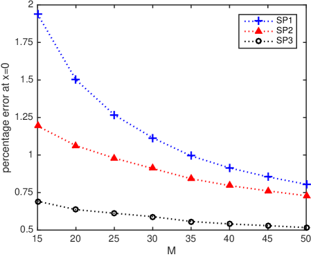
Figure 1: Error of the nonclassical SP_N estimates for the scalar flux with respect to the benchmark solution at $x=0$.

The expectation is that the estimates obtained with the nonclassical SP_N theory as given by Eq. 29 to (32) will increase in accuracy as $M$ increases and $\varepsilon\rightarrow 0$. Figure 1 shows the percent relative error of the nonclassical SP_N estimates with respect to the benchmark results, calculated at the center of the system ($x=0$) for different values of $M$.

As anticipated, the numerical results confirm the asymptotic analysis: (i) the accuracy of the SP_N equations increases as $N$ increases; and (ii) for each choice of $N$, the error decreases as $M$ increases and the system approaches the diffusive limit.

VI Conclusions

In this paper we have derived a set of diffusion approximations to the nonclassical transport equation with isotropic scattering using a high-order asymptotic expansion. These approximations reduce to the simplified P_N equations under the assumption of classical transport, and for that reason are labeled nonclassical SP_N equations. Explicit equations are given for nonclassical SP₁ (diffusion), SP₂, and SP₃; higher-order equations can be derived by continuing to follow the same procedure. The caveat of this analysis is that the first $2M$ raw moments of the free-path distribution $p(s)$ are required to be finite in order to obtain the nonclassical SP_N equations for $N=M$.

Although the analysis does not yield boundary conditions, we show that the nonclassical SP_N equations can be manipulated into a classical form with modified parameters. This allows us to generate numerical results using Marshak vacuum boundary conditions. More importantly, by using this approach one can implement the nonclassical SP_N equations in existing SP_N codes.

Numerical results for a 1-D random periodic system are presented, validating the theoretical predictions. This result paves the road to a more complete understanding of the diffusive behavior of the nonclassical transport theory. Future work includes (i) performing numerical calculations in nonclassical multi-dimensional systems; (ii) extending the asymptotic analysis to include angular-dependent free-path distributions; and (iii) extending the analysis to include anisotropic scattering.

VII Acknowledgments

This paper was prepared by R. Vasques and R. N. Slaybaugh under award number NRC-HQ-84-14-G-0052 from the Nuclear Regulatory Commission. The statements, findings, conclusions, and recommendations are those of the authors and do not necessarily reflect the view of the U.S. Nuclear Regulatory Commission.

References

• [1] E. W. LARSEN, “A generalized Boltzmann equation for non-classical particle transport,” in Proceedings of the International Topical Meeting on Mathematics & Computation and Supercomputing in Nuclear Applications, Monterey, CA, 2007.
• [2] E. W. LARSEN and R. VASQUES, “A generalized linear Boltzmann equation for non-classical particle transport,” Journal of Quantitative Spectroscopy and Radiative Transfer, 112, 619 (2011).
• [3] R. VASQUES and E. W. LARSEN, “Non-classical particle transport with angular-dependent path-length distributions. II: Application to pebble bed reactor cores,” Annals of Nuclear Energy, 70, 301 (2014).
• [4] A. B. DAVIS and F. XU, “A generalized linear transport model for spatially correlated stochastic media,” Journal of Computational and Theoretical Transport, 43, 474 (2014).
• [5] E. D’EON, “Rigorous asymptotic and moment-preserving diffusion approximations for generalized linear boltzmann transport in arbitrary dimension,” Transport Theory and Statistical Physics, 42, 237 (2013).
• [6] M. FRANK and T. GOUDON, “On a generalized Boltzmann equation for non-classical particle transport,” Kinetic and Related Models, 3, 395 (2010).
• [7] E. M. GELBARD, “Applications of spherical harmonics method to reactor problems,” WAPD-BT-20, Bettis Atomic Power Laboratory (1960).
• [8] E. M. GELBARD, “Simplified spherical harmonics equations and their use in shielding problems,” WAPD-T-1182, Bettis Atomic Power Laboratory (1961).
• [9] E. M. GELBARD, “Applications of simplified spherical harmonics equations in spherical geometry,” WAPD-TM-294, Bettis Atomic Power Laboratory (1962).
• [10] E. W. LARSEN, J. E. MOREL, and J. M. MCGHEE, “Theoretical aspects of the simplified PN equations,” in Proceedings of the ANS Topical Meeting on Mathematical Methods and Supercomputing in Nuclear Applications, Karlsruhe, Germany, 1993.
• [11] R. G. MCCLARREN, “Theoretical aspects of the simplified PN equations,” Transport Theory and Statistical Physics, 39, 73 (2011).
• [12] M. FRANK, A. KLAR, E. W. LARSEN, and S. YASUDA, “Time-dependent simplified PN approximation to the equations of radiative transfer,” Journal of Computational Physics, 226, 2289 (2007).
• [13] D. I. TOMASEVIC and E. W. LARSEN, “The simplified P2 approximation,” Nuclear Science and Engineering, 122, 309 (1996).
• [14] O. ZUCHUAT, R. SANCHEZ, I. ZMIJAREVIC, and F. MALVAGI, “Transport in renewal statistical media: benchmarking and comparison with models,” Journal of Quantitative Spectroscopy and Radiative Transfer, 51, 689 (1994).
• [15] R. VASQUES, K. KRYCKI, and R. N. SLAYBAUGH, “Nonclassical particle transport in one-dimensional random periodic media,” Nuclear Science and Engineering, 185, 78 (2017).