Systematic Study of Gamma-ray bright Blazars with Optical Polarization and Gamma-ray Variability

Abstract

Blazars are highly variable active galactic nuclei which emit radiation at all wavelengths from radio to gamma-rays. Polarized radiation from blazars is one key piece of evidence for synchrotron radiation at low energies and it also varies dramatically. The polarization of blazars is of interest for understanding the origin, confinement, and propagation of jets. However, even though numerous measurements have been performed, the mechanisms behind jet creation, composition and variability are still debated.

We performed simultaneous gamma-ray and optical photopolarimetry observations of 45 blazars between Jul. 2008 and Dec. 2014 to investigate the mechanisms of variability and search for a basic relation between the several subclasses of blazars. We identify a correlation between the maximum degree of optical linear polarization and the gamma-ray luminosity or the ratio of gamma-ray to optical fluxes. Since the maximum polarization degree depends on the condition of the magnetic field (chaotic or ordered), this result implies a systematic difference in the intrinsic alignment of magnetic fields in pc-scale relativistic jets between different types blazars (FSRQs vs. BL Lacs), and consequently between different types of radio galaxies (FR Is vs. FR IIs).

1. Introduction

Blazars are a subclass of active galactic nuclei (AGNs) possessing relativistic jets, which are extremely powerful and fast outflows of plasma that emerge from the vicinity of the massive black hole. Their observed emission is dominated by the contributions of relativistic jets aligned with the observer’s line of sight resulting in a strong apparent boost due to relativistic beaming. Outstanding characteristics of blazars are their rapid and high-amplitude intensity variations. The apparent bolometric luminosity of blazars can be as high as $10^{48}$ erg s^-1 (see, e.g., Urry & Padovani, 1995). The overall spectral energy distribution consists of at least two broad non-thermal components, the low-energy one attributed to synchrotron radiation, and the high-energy one attributed to inverse Compton scattering. Since the non-thermal emission from jets is dominant compared to the thermal emission from the disk due to relativistic effects, blazars are some of the most suitable objects to study the relativistic jets.

Depending on the behavior in optical spectra or in the peak frequency of synchrotron radiation, blazars are divided into different sub-classes. Flat spectrum radio quasars (FSRQs) are defined to have strong emission lines of equivalent width $>5\$Å in the observer’s optical band (Stickel et al., 1991). In contrast, BL Lac objects show relatively weak emission lines. Additionally, blazars can be classified into three types based on their peak frequency of synchrotron radiation $\nu_{\rm peak}^{S}$: low-synchrotron-peaked blazars (LSP; for sources with $\nu_{\rm peak}^{S}<10^{14}$ Hz), intermediate-synchrotron-peaked blazars (ISP; for $10^{14}\;{\rm Hz}<\nu_{\rm peak}^{S}<10^{15}$ Hz), and high-synchrotron-peaked blazars (HSP; for $10^{15}\;{\rm Hz}<\nu_{\rm peak}^{S}$) (Ackermann et al., 2011, 2015b). Essentially most of FSRQs are LSPs (only three FSRQ-HSP and several FSRQ-ISP are reported in Ackermann et al., 2015b), while BL Lacs can be LSPs, ISPs or HSPs. According to the blazar sequence, the synchrotron luminosity $L_{\rm syn}$, the inverse Compton luminosity $L_{\rm IC}$, and also the ratio of these two luminosities $q=L_{\rm IC}/L_{\rm syn}$ are inversely correlated with the synchrotron peak frequency $\nu_{\rm peak}^{S}$ (Fossati et al., 1998). Hence, the FSRQs are both more luminous and more Compton dominated (higher $q$ value) than the BL Lacs. Ghisellini et al. (1998) provided a physical explanation for this spectral sequence, proposing that it originated from radiative electron cooling in the jet. A unified model of Urry & Padovani (1995) has become generally accepted, whereas FSRQs are related to intrinsically powerful (FR II) radio galaxies, and BL Lac objects are related to intrinsically weak (FR I) radio galaxies. The two types of radio galaxies also possess jets, but those are directed farther away from our line of sight.

Mead et al. (1990) performed a large-sample study of blazars in the optical band and showed that high polarization degree and variability of polarization are common phenomena in blazars: this, together with the high level of polarization observed in the radio band, provides strong support for the synchrotron radiation as an origin of the low energy emission. The level, but also the position angle of polarization (electric vector position angle, the direction is measured from north to east) in blazars often varies dramatically, and these are important ingredients for understanding the origin, confinement, and propagation of jets (e.g., Brand, 1985; Visvanathan & Wills, 1998). Ikejiri et al. (2011, hereafter Paper I), reported the statistics of photopolarimetric observations of blazars on daily timescales, and suggested that sources characterized by lower luminosity, and those with the peak of the synchrotron radiation located at higher frequencies (such as HSPs) had smaller amplitude variations in the flux, color, and polarization degree. These authors also reported that about 30% of blazars showed a correlation between the optical flux and polarization degree. Polarization depends on the structure of the magnetic field in the emitting region, and thus polarimetric observations of blazars in the optical band are valuable for probing the magnetic fields in relativistic AGN jets at (sub-)pc scales since the optical emission region is thought to be located at pc-scales from central engine (e.g., Marscher et al., 2008; Agudo et al., 2011). Rotations of polarization angle during flares are also important observational phenomena in blazars (e.g. Marscher et al., 2008; Blinov et al., 2015). However, the details need to be dealt with carefully, because some apparent rotations might be caused by random variation of polarization on the Stokes parameter QU plane (e.g. Jones et al., 1985; Kiehlmann et al., 2016).

Very few attempts have been made to systematically study variability, especially focusing on multi-wavelength and polarimetric observations amongst the several subclasses of blazars (Blinov et al., 2015). In this paper, we search for a basic relation between gamma-ray properties and optical flux and polarization with a systematic study of 45 blazars to investigate the mechanisms of variability.

2. Observations

2.1. Optical Observations with Kanata

We performed optical and near infrared imaging polarimetry of 42 AGNs between Aug. 2008 and Dec. 2014 with the 1.5m diameter Kanata Telescope. We used two instruments attached to the Kanata telescope: one is TRISPEC (Triple Range Imager and SPECtrograph; Watanabe et al., 2005) and the other is HOWPol (Hiroshima One-shot Wide-field Polarimeter; Kawabata et al., 2008). TRISPEC was attached to the Cassegrain focus of the Kanata telescope from 2006 to 2011 and it has a CCD and two InSb arrays, enabling photopolarimetric observations in one optical and two near-infrared bands simultaneously. HOWPol is installed at the Nasmyth focus of the Kanata telescope, and has been in operation since 2009.

We performed V, J, Ks-band photometry and polarimetry observations of each target from July 2008 to February 2010 using TRISPEC and performed the V and R_C-band photometry and polarimetry observations from July 2008 to February 2010 using HOWPol. Each observing sequence consisted of successive exposures at four position angles of a half-wave plate of $0^{\circ},45^{\circ},22.5^{\circ}$ and $67.5^{\circ}$.

The data reduction involved standard CCD photometry procedures — aperture photometry using APPHOT package in PYRAF and differential photometry with a comparison star taken in the same frame. The positions of the comparison stars are listed in Table 1. The data have been corrected for Galactic extinction (values are given in Table 1). We confirmed that the instrumental polarization was smaller than 0.1% in the V band (TRISPEC), using unpolarized standard stars and thus applied no correction for it. The polarization angle (PA) is defined in the standard manner (measured from north to east), and it was calibrated with two polarized stars, HD19820 and HD25443 (Wolff et al., 1996). The time series data of V, R_C, J, Ks-band photometry and V, R_C-band polarimetry will be available via Centre de Données astronomiques de Strasbourg (CDS, Strasbourg astronomical Data Center ).

Polarimetry with HOWPol suffers from large instrumental polarization ($\Delta p\sim 4$%) produced by the reflection of the incident light on the tertiary mirror of the telescope. The instrumental polarization was modeled as a function of the declination of the object and the hour angle at the observation, and we subtracted it from the observation. We estimated that the error in this instrumental polarization correction is smaller than $\Delta p\sim 0.5$% from many observations of unpolarized standard stars. The PA was calibrated using two polarized stars, HD183143 and HD204827 (Schulz & Lenzen, 1983). We also confirmed that systematic differences in the photometric and polarimetric systems are negligibly small by measurements of comparison stars.

Table 1List of comparison stars

Source Name	Comparison Coordinates	$V$	$R_{C}$	$J$	$Ks$	A(V)	Ref.
(1)	(2)	(3)	(4)	(5)	(6)	(7)	(8)
PKS 0048-097	00:50:47.0 -09:30:15.0	14.096	13.741	12.455	11.854	0.104	[1],[2]
S2 0109+22	01:12:03.0 +22:43:26.0	12.477	12.272	11.245	10.886	0.122	[1],[2]
Mis V1436	01:36:42.0 +47:51:03.0	13.394	13.272	12.223	11.922	0.496	[1],[2]
PKS 0215+015	02:17:49.0 +01:48:28.0	12.156	12.076	11.320	11.046	0.108	[1],[2]
3C 66A	02:22:55.1 +43:03:15.5	13.183	13.314	12.371	12.282	0.274	[3],[4]
AO 0235+164	02:38:32.0 +16:36:00.0	12.756	12.523	11.248	10.711	0.258	[1],[2]
1H 0323+342	03:24:39.0 +34:11:29.0	13.445	12.773	–	–	0.680	[1]
	03:24:33.0 +34:10:53.0	13.221	–	11.232	10.589	0.680	[3],[2]
1ES 0323+022	03:26:13.4 +02:24:06.1	12.840	–	11.097	10.485	0.551	[5]
PKS 0422+00	04:24:42.4 +00:37:10.8	12.510	–	11.217	10.899	0.338	[5]
PKS 0454-234	04:57:00.0 -23:26:05.0	12.359	12.149	10.849	10.364	0.149	[1],[2]
1ES 0647+250	06:50:40.0 +25:03:24.0	13.060	12.921	12.053	11.771	0.320	[1],[2]
S5 0716+714	07:21:54.0 +71:19:20.0	13.468	13.367	–	–	0.101	[1]
	07:21:52.2 +71:18:16.1	12.345	–	11.320	10.980	0.101	[3],[4]
4C 14.23	07:25:20.0 +14:25:03.0	14.842	14.637	–	–	0.284	[1]
PKS 0735+17	07:38:02.0 +17:41:21.0	14.170	13.991	–	–	0.110	[1]
PKS 0754+100	07:57:16.1 +09:55:47.8	13.000	–	11.852	11.496	0.071	[4]
1ES 0806+524	08:09:40.0 +52:19:17.0	12.999	12.741	11.417	10.867	0.146	[1],[5]
OJ 49	08:31:54.0 +04:30:43.0	13.550	13.429	–	—	0.106	[1]
	08:32:00.7 +04:32:02.5	13.517	–	12.475	12.189	0.106	[3],[5]
OJ 287	08:54:53.0 +20:04:44.0	14.190	13.929	–	–	0.092	[1]
	08:54:59.0 +20:02:57.1	13.954	13.832	12.811	12.445	0.092	[3],[4]
PMN J0948+022	09:49:10.0 +00:21:40.0	14.983	14.732	13.500	13.139	0.253	[1],[2]
S4 0954+65	09:58:50.4 +65:32:09.1	14.610	–	12.927	12.455	0.372	[5]
Mrk 421	11:04:18.2 +38:16:30.5	15.570	15.200	14.453	14.106	0.050	[6]
ON 325	12:17:44.0 +30:09:43.0	15.097	14.871	13.674	13.232	0.075	[1],[2]
1ES 1218+304	12:21:31.0 +30:11:00.0	12.400	10.489	–	–	3.240	[7]
ON 231	12:21:33.0 +28:13:04.0	12.071	11.965	10.921	10.597	0.076	[1],[2]
3C 273	12:29:08.0 +02:00:18.0	12.725	12.540	11.345	10.924	0.067	[1],[4]
GB6 J1239+0443	12:39:30.1 +04:39:52.6	14.095	–	12.942	12.638	0.072	[8]
3C 279	12:56:10.0 -05:50:14.0	12.420	12.257	–	–	0.093	[1]
	12:56:16.9 -05:50:43.0	13.517	13.318	12.377	11.974	0.093	[3],[9]
OQ 530	14:20:18.0 +54:24:14.0	14.357	14.189	–	–	0.043	[1]
	14:19:39.7 +54:21:55.0	16.009	–	13.873	13.131	0.043	[3],[8]
PKS 1502+106	15:04:13.0 +10:28:42.0	14.552	14.331	–	–	0.104	[1]
	15:04:36.5 +10:28:47.0	15.328	–	14.117	13.678	0.104	[3],[5]
PKS 1510-089	15:12:51.0 -09:05:23.0	14.630	14.466	–	–	0.327	[1]
	15:12:53.2 -09:03:43.6	13.195	–	12.205	11.919	0.327	[3],[4]
RX J1542.8+612	15:42:39.0 +61:30:26.0	13.958	13.303	9.640	–	0.052	[1],[4]
PG 1553+113	15:55:52.0 +11:13:18.0	13.842	13.625	12.539	12.139	0.169	[1],[9]
3C 345	16:42:52.0 +39:48:33.0	15.304	14.963	–	–	0.043	[1]
Mrk 501	16:53:45.0 +39:44:09.0	12.534	12.195	10.935	10.399	0.061	[1],[4]
H1722+119	17:25:05.0 +11:52:10.0	13.214	12.828	11.308	10.710	0.559	[1],[5]
NRAO 530	17:33:00.0 -13:04:09.0	14.488	13.851	–	–	1.699	[1]
PKS 1749+096	17:51:31.0 +09:39:40.0	14.278	14.014	–	–	0.577	[1]
	17:51:37.3 +09:39:07.1	11.857	–	10.252	9.740	0.577	[3],[5]
S5 1803+784	17:59:52.6 +78:28:50.9	13.133	12.226	11.761	11.381	0.169	[7],[10]
3C 371	18:07:12.0 +69:47:07.0	14.127	13.900	–	–	0.109	[1]
	18:06:53.7 +69:45:37.4	13.254	–	12.219	11.856	0.109	[3],[4]
1ES 1959+650	19:59:39.2 +65:08:52.9	14.618	11.301	–	–	0.557	[7]
	20:00:26.5 +65:09:26.4	13.180	–	11.464	11.315	0.557	[6]
PKS 2155-304	21:59:02.5 -30:10:46.2	12.050	–	10.775	10.365	0.071	[4]
BL Lac	22:02:45.0 +42:16:35.0	12.939	12.326	9.817	8.811	1.063	[1],[4]
CTA 102	22:32:41.0 +11:43:14.0	15.347	14.971	–	–	0.233	[1]
3C 454.3	22:53:58.0 +16:09:06.0	13.661	13.342	11.858	11.241	0.349	[1],[4]
1ES 2344+514	23:47:02.2 +51:43:17.6	12.565	12.177	11.421	11.117	0.680	[7],[5]

(1) Object name. (2) Coordinate of comparison stars. (3), (4), (5), (6) V, R, J, Ks band magnitudes of comparison stars. (7) Galactic extinction for V-band. (8) Reference for the magnitudes of comparison stars. [1];UCAC-4 catalog, [2];2MASS catalog, [3];Calibrated with UCAC-4, [4]Gonzalez-Perez+01, [5];Skiff+05, [6];Villata+98, [7];UCAC-3, [8];Adelman-McCarthy+07, [9];Doroshenko+05, [10];Zacharias+05

2.2. Gamma-ray Observations with Fermi

The Fermi Gamma-ray Space Telescope is an observatory in a low-Earth orbit launched on 2008 June 11. The Large Area Telescope (LAT) is the instrument used for monitoring high-energy (MeV to GeV) emission of AGN and other sources. It is an electron-positron pair production detector with a bandpass of 20 MeV - 300 GeV, described in detail in Atwood et al. (2009). The LAT observes the whole sky every 3 hours with a large effective area of $8000$ cm² at 1 GeV, a wide field of view of $2.4$ sr, and a single photon angular resolution (68% containment radius) of $0.6^{\circ}$ at 1 GeV.

The data used in this analysis were taken between 2008 August and 2014 December, almost entirely in sky survey mode. The data were analyzed using the standard Fermi analysis software (Science Tools, version v10r00, IRFs P8$\_$R2). We use Pass 8 “Source” class event data above 100 MeV. We also restricted our analysis to events with zenith angles $<90^{\circ}$ to limit the contamination by gamma-rays from the Earth’s limb. We performed an Unbinned Likelihood analysis to calculate the gamma-ray spectrum and flux of our targets, using the gtlike package in the Science Tools. An area of $15^{\circ}$ around target was selected as a region of interest (ROI) for this analysis. We constructed a model of the ROI that includes a point source at the position of each target. We modeled the spectrum of each blazar as a power-law:

$$\frac{dN}{dE}=N_{0}\left(\frac{E}{E_{0}}\right)^{-\alpha}$$ (1)

where $N_{0}$ is the normalization at energy $E_{0}$ and $\alpha$ is the photon index. The flux normalization and spectral index were left free in the likelihood analysis. We constructed the background source model based on the 3FGL catalog (Acero et al., 2015, LAT 4-year Point Source Catalog). The spectral indicies of the background sources were fixed to their catalog values while their normalizations were left free. The Galactic diffuse emission component (gll_iem_v06.fit, Acero et al., 2016) and the isotropic diffuse emission component (iso_P8R2_SOURCE_V6_v06.txt) are included in our models. We performed the model fitting in twice. First, all the 3FGL sources in the ROI were included in the model and fitted over the 7-day intervals. We then fit a second model with the background sources with low test statistics ($TS<25$) omitted from the data.

2.3. Data selection for systematic studies

The purpose of this study is to search for a basic relation between the blazars sub classes. Both gamma-ray and optical band data possess observational gaps due to low photon statistics, bad weather, visibility and maintenance of instruments. Some parameters, like the variability index (see below for the definition), are dependent on their observational periods. In order to compare such parameters between the gamma-ray and optical band, we selected strictly simultaneous data from our sample. Specifically, we excluded the gamma-ray data which have no counterpart in optical observations. We also extracted the optical data which have no significant gamma-ray detection ($TS<25$). Since the bin size of the gamma-ray data was set to 7 days, we also averaged the optical data to match the gamma-ray bins for the DCF analysis (Section 3.3) and the derivation of the ratio between gamma-ray flux and optical flux. The unaveraged data were used in all other cases. We note that there are several uncertainties in the calculation of the time lag since averaging the optical data may make some temporal bias since the observational time of gamma-ray does not necessarily correspond to average time of optical data. Thus, we do not discuss time lags less than 3.5 days in this paper. Among 45 blazars, we selected 24 targets for our systematic studies, which have more than 10 simultaneous gamma-ray and optical data points. These targets are listed in Table 2.

Table 2List of our targets with more than 10 data points.

Object Name	3FGL name	$\log(v_{\rm peak})$	Type	z	$N_{\rm opt.}$	$N_{\rm\gamma}$
(1)	(2)	(3)	(4)	(5)	(6)	(7)
S2 0109+22	3FGL J0112.1+2245	14.6	ISP	0.265	44	24
Mis V1436	3FGL J0136.9+4751	13.6	LSP (FSRQ)	0.859	52	18
3C 66A	3FGL J0222.6+4302	15.1	ISP	0.444	462	164
AO 0235+164	3FGL J0238.7+1637	13.5	LSP	0.94	72	26
PKS 0454-234	3FGL J0457.0-2325	13.1	LSP (FSRQ)	1.003	27	20
S5 0716+714	3FGL J0721.9+7120	14.6	ISP	0.3	556	198
OJ 49	3FGL J0831.9+0429	13.5	LSP	0.1737	27	16
OJ 287	3FGL J0854.8+2005	13.4	LSP	0.306	174	75
Mrk 421	3FGL J1104.4+3812	16.6	HSP	0.031	85	46
ON 325	3FGL J1217.8+3006	15.5	HSP	0.13	38	17
3C 273	3FGL J1229.1+0202	13.5	LSP (FSRQ)	0.15834	224	91
3C 279	3FGL J1256.1-0547	12.6	LSP (FSRQ)	0.5362	140	72
PKS 1502+106	3FGL J1504.3+1029	13.6	LSP (FSRQ)	1.839	71	27
PKS 1510-089	3FGL J1512.8-0906	13.1	LSP (FSRQ)	0.36	108	51
RX J1542.8+612	3FGL J1542.9+6129	14.1	LSP (FSRQ)	0.117	69	38
PG 1553+113	3FGL J1555.7+1111	15.4	HSP	0.36	196	90
Mrk 501	3FGL J1653.9+3945	17.1	HSP	0.033663	170	80
PKS 1749+096	3FGL J1751.5+0938	13.1	LSP (FSRQ)	0.322	47	16
3C 371	3FGL J1806.7+6948	14.7	ISP (FSRQ)	0.051	21	16
1ES 1959+650	3FGL J2000.0+6509	16.6	ISP	0.047	82	42
PKS 2155-304	3FGL J2158.8-3013	16.0	HSP	0.116	146	60
BL Lac	3FGL J2202.8+4216	13.6	LSP	0.0686	340	137
CTA 102	3FGL J2232.4+1143	13.6	LSP (FSRQ)	1.07	76	33
3C 454.3	3FGL J2253.9+1609	13.6	LSP (FSRQ)	0.859	442	143

(1) Object name. (2) object name in 3FGL catalog. (3) Synchrotron peak frequency. (4) blazar type. (5) redshift of object from the NASA/IPAC Extragalactic Database (NED). (6) Number of simultaneous optical ($V$-band) data point. (7) Number of simultaneous GeV data point.

3. Results

There are a lot of evaluation methods of blazar properties, such as measurement of variability index, correlation between gamma-ray and optical properties. In addition to these, blazars have various characteristics such as luminosity, redshift and synchrotron peak frequency. The question we have to ask here is what are common properties in blazars. In this section, we describe results with several blazar properties which might be good elements of a new blazar classification scheme.

3.1. Light curves

In this section, we report on the results of our observations. In Figure 1, we show the temporal variation of the gamma-ray flux, gamma-ray index, optical flux, ratio of gamma-ray to optical fluxes, polarization degree, and polarization angle for the source S5 0716+714. The ratio of gamma-ray to optical fluxes is derived from the gamma-ray $\nu F_{\nu}$ value at 100 MeV and from the optical $\nu F_{\nu}$ value in the V-band. This ratio is similar to the Compton dominance (e.g., Finke, 2013), although an accurate value of the Compton dominance should be calculated from the integrated fluxes of synchrotron and inverse Compton components. This ratio can be a good indicator of conditions in the blazar jet, because it is only weakly redshift dependent. Since both the gamma-ray and optical fluxes show dramatic variability, observation of both fluxes should be simultaneous as much as possible. In this paper, we present data for a number of blazars; analogous plots for all 24 objects, for completeness including S5 0716+714, are shown in Appendix A.

There are several types of variability in different bands. For example, S5 0716+714 shows many high-amplitude flares at very short intervals (this is also suggested in Sasada et al., 2008). In contrast, in the case of PKS 1510-089 we rarely observe very prominent flares, which consist of a small number of subcomponents (see Fig. 21). The cadence and the amplitudes of flares in PKS 1510-089 are also different from those in S5 0716+714. In order to compare the properties of such different types of flares, we investigate the observed photo-polarimetric variability in several ways.

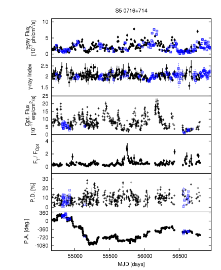
Figure 1.— Temporal variability of gamma-ray flux, gamma-ray index, optical flux, ratio of gamma-ray flux, polarization degree and polarization angle for the source S5 0716+714. The top panel shows the gamma-ray light curve, the second panel shows variability of gamma-ray spectral index, the third panel shows the optical V-band light curve, the fourth panel shows ratio of gamma-ray to optical flux, the fifth panel shows variability of polarization degree and bottom panel shows variability of polarization angle. Black-filled data points indicates the data with simultaneous optical polarization and gamma-ray observations that we used in our analysis. Blue-opened box data points indicate the excluded data in our analysis (see Sec 2.3 for data selection).

3.2. Variability of polarization in the Stokes parameter (Q,U) plane

Information on linear polarization can be represented in several ways. Polarization degree $\Pi$ can be combined with the total flux $I$ to yield the polarized flux $\Pi I$. Polarization angle $\chi$ can be combined with the polarized flux to yield the Stokes parameters $Q=\Pi I\cos(2\chi)$ and $U=\Pi I\sin(2\chi)$. Namely, when plotted on the ($Q/I,U/I$) plane, the distance of an individual point from the origin corresponds to $\Pi$, and the direction of ($Q/I,U/I$) vector from $Q/I$ axis correspond to $2\chi$. In some cases, blazars show a clear correlation between total optical flux and polarization degree, but sometimes they do not show such correlation. It is known that variability of polarization of blazars does not show simple, symmetrical motion but shows complex motion in the $(Q,U)$ plane (e.g. Uemura et al., 2010). In addition, polarization angle has an ambiguity of $\pm 180n$ degree (where $n$ is an integer) and this makes it difficult to measure the variability of polarization angle. Therefore, it is important to evaluate the variability of polarization in the $(Q,U)$ plane. The purpose of this analysis is to clarify the distribution of polarization in the $(Q,U)$ plane and uniformity of polarization variability. In order to compare the polarization variability properties between individual sources, we adopted an ellipsoidal variance measurement to characterize the distribution of the observed polarization in the $(Q,U)$ plane. First, we calculated the median values of $Q_{0}$ and $U_{0}$ in order to determine the slope of major axis of the distribution, then we performed a two-dimensional least-squares fit to the observed values of $Q-Q_{0}$ and $U-U_{0}$, which yields the correlation coefficient, the mean polarization angle $\chi_{0}$ corresponding to the inclination of the major axis of the distribution, and also the variance values measured along the major and minor axes. An example of such ellipsoidal variance for the source OJ 287 is shown in Figure 2. From this figure, one can see that the average values of $Q_{0}$ and $U_{0}$ are clearly not coincident with the origin of the $(Q,U)$ plane, and that the distribution of $Q$ and $U$ is asymmetric with respect to point ($Q_{0},U_{0}$). A summary of ellipsoidal variance measurement results for all sources is presented in Table 3.

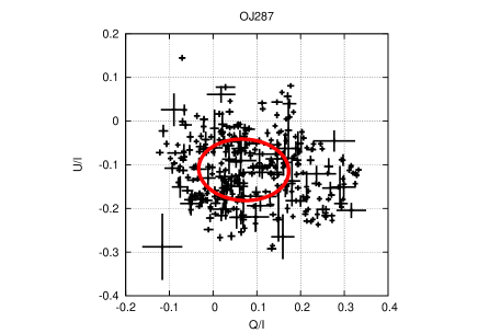
Figure 2.— Left panel; Elliptical fitting in the QU plane for the source OJ 287. Length of major and minor axes of distribution indicates the variation (1-$\sigma$) of polarization in two-dimensional space. Right panel; temporal variability of Q/I and U/I plot for the same source.

Table 3Summary of variability of polarization on the Stokes parameter QU plane

Source Name	$Q_{0}^{(1)}$	$U_{0}^{(2)}$	$\chi_{0}^{(3)}$ [deg.]	$\sigma_{\rm major}^{(4)}$	$\sigma_{\rm minor}^{(5)}$
S2 0109+22	-0.04	-0.03	0.4	0.06	0.10
Mis V1436	-0.12	0.05	1.4	0.15	0.07
3C 66A	0.07	0.07	-0.2	0.04	0.05
AO 0235+164	-0.08	0.00	-14.5	0.11	0.08
PKS 0454-234	0.02	-0.03	25.9	0.11	0.10
S5 0716+714	-0.02	0.02	-1.1	0.07	0.07
OJ 49	-0.03	-0.03	2.5	0.05	0.06
OJ 287	0.06	-0.11	-2.6	0.10	0.07
Mrk 421	0.01	-0.01	3.2	0.02	0.02
ON 325	0.07	-0.03	-33.5	0.04	0.03
3C 273	0.00	0.00	1.0	0.00	0.00
3C 279	-0.06	0.08	-9.9	0.10	0.11
PKS 1502+106	-0.04	-0.15	-37.5	0.16	0.11
PKS 1510-089	0.01	0.00	13.1	0.05	0.07
RX J1542.8+612	0.03	0.02	-20.2	0.05	0.04
PG 1553+113	-0.01	-0.01	2.7	0.02	0.03
Mrk 501	0.00	-0.01	-13.7	0.01	0.01
PKS 1749+096	-0.01	-0.01	34.6	0.10	0.09
3C 371	-0.06	0.02	37.0	0.03	0.02
1ES 1959+650	0.02	-0.03	-6.8	0.02	0.02
PKS 2155-304	-0.02	0.02	-22.5	0.03	0.03
BL Lac	0.07	0.04	-3.6	0.06	0.05
CTA 102	0.00	0.03	10.7	0.06	0.08
3C 454.3	0.01	-0.01	-3.7	0.06	0.05

(1),(2); Median value of $Q$ and $U$, (3); mean polarization angle, (4),(5) the variance values measured along the major and minor axes.

3.3. Correlation between gamma-ray and optical light curves

Temporal correlations between various gamma-ray and optical properties can be quantified by calculating the Discrete Correlation Function (Edelson & Krolik, 1988, DCF). Since the bin size of the gamma-ray data were was set to 7 days, we also averaged the optical fluxes to match the gamma-ray bins for the DCF analysis (Section 3.3) and the derivation of ratio between gamma-ray flux and optical flux. The unaveraged data were used in all other cases, and specifically in reporting the polarization degree and angle. Figure 3 shows a scatter plot of gamma-ray flux vs optical fluxes for 3C 454.3. In this case, this source shows significant correlation between gamma-ray flux and optical flux with no significant time lag. We measured the correlations corresponding to zero time lag for all our samples. The error of DCF values are estimated from the variance of the data for each time-lag interval. In fact, there are several sources which show good correlation between gamma-ray and optical fluxes, which actually do show time lags (e.g., PKS 1510-089 Nalewajko et al., 2012). For PG 1553+113, correlation between gamma-ray flux and optical flux with time lag is due to a possible 2-year periodic modulation (Ackermann et al., 2015a). Figure 4 shows the DCF plot for 11 blazars which possess enough data to calculate the correlation coefficient in several time intervals and show significant correlations or anti-correlations within the -200 to 200 day time lag window. Summary of time lag and correlation coefficient for those 11 blazars are listed in Table 4. The significance of the correlation (95% C.L.) was tested using the block Bootstrap method. In this method, we randomly resampled the data and calculated the correlation coefficient with replacement. We repeat this routine 10,000 times to get the Bootstrap distribution for each dataset. From this Bootstrap distribution, we derived a confidence intervals of $\alpha$ = 0.95 (see Appendix B). Uncertainties in the time lag are derived by the period that shows significance of correlation (95% C.L.). Some of them show asymmetrical shapes in the DCF plot, which might be related to the difference of rise/decay of the gamma-ray flare and the optical flare (e.g. 3C 454.3), however, the physical origin of time lags between gamma-ray and optical features is still unclear (e.g., Janiak et al., 2012) and both delayed and precursory gamma-ray flares against optical flares are observed in blazars. To simplify the discussion and to increase the sample, we use the correlations corresponding to zero time lag. We adopt the DCF value for zero time lag as the correlation index. We systematically investigated the correlations between gamma-ray flux and optical flux, polarization degree and polarized flux with zero time lag.

Figure 3.— Scatter plot of gamma-ray flux and optical flux for 3C 454.3. The optical data were averaged with 7-day intervals. Error bars for the optical data indicate the 1-$\sigma$ variance of 7-day interval data. The Figure shows significant correlation between gamma-ray flux and optical flux with no time lag (also see Figure 4 and Table 4).

Figure 4.— DCF plot of gamma-ray flux and optical flux for several blazars. Significant peak of each source are listed in Table 4.

Table 4Summary of Correlation time lags between gamma-ray flux and optical flux

Source Name	time lag (days)	DCF peak value
AO 0235+164	0 ${}^{+4}_{-14}$	0.67 $\pm$ 0.08
S5 0716+714	0 $\pm 7$	0.47 $\pm$ 0.05
OJ 287	-134 ${}^{+4}_{-28}$	1.0 $\pm$ 0.5
3C 273	-145 ${}^{+7}_{-21}$	-0.97 $\pm$ 0.18
3C 279	-28 $\pm 14$	0.67 $\pm$ 0.15
3C 279	77 ${}^{+7}_{-14}$	-0.6 $\pm$ 0.1
PG 1553+113	21 ${}^{+14}_{-28}$	0.4 $\pm$ 0.1
PKS 2155-304	-28 ${}^{+28}_{-7}$	0.9 $\pm$ 0.2
BL Lac	$0^{+28}_{-77}$	1.0 $\pm$ 0.1
CTA 102	0 $\pm 7$	0.8 $\pm$ 0.2
3C 454.3	$0^{+49}_{-49}$	0.84 $\pm$ 0.13

Table 5Summary of Correlations

Source Name	$L_{\rm gamma}^{1}$	$L_{\rm opt}^{2}$	$R_{gamma-opt}^{3}$	PD${}_{\rm max}^{4}$	V${}_{\rm gamma}^{5}$	V${}_{\rm opt}^{6}$	V${}_{\rm PD}^{7}$	DCF${}_{\rm gamma-opt}^{8}$	DCF${}_{\rm opt-PD}^{9}$
S2 0109+22	45.31	45.53	0.61 $\pm$ 0.30	22.75 $\pm$ 0.69	0.39 $\pm$ 0.10	0.22 $\pm$ 0.01	$0.52\pm 0.02$	0.02 $\pm$ 0.09	-0.25 $\pm$ 0.09
Mis V1436	46.87	45.98	6.73 $\pm$ 2.45	33.68 $\pm$ 1.07	0.28 $\pm$ 0.09	0.47 $\pm$ 0.01	$0.52\pm 0.03$	0.47 $\pm$ 0.23∗	0.58 $\pm$ 0.07∗
3C 66A	45.84	45.94	0.78 $\pm$ 0.28	24.76 $\pm$ 0.27	0.26 $\pm$ 0.03	0.31 $\pm$ 0.01	$0.39\pm 0.01$	0.36 $\pm$ 0.09∗	0.05 $\pm$ 0.02
AO 0235+164	47.40	46.58	8.16 $\pm$ 1.57	33.80 $\pm$ 1.86	0.46 $\pm$ 0.03	0.83 $\pm$ 0.01	$0.57\pm 0.03$	0.67 $\pm$ 0.08∗	0.84 $\pm$ 0.08∗
PKS 0454-234	47.50	46.65	7.51 $\pm$ 1.18	29.98 $\pm$ 1.58	0.43 $\pm$ 0.04	–	$0.61\pm 0.02$	0.12 $\pm$ 0.04∗	0.06 $\pm$ 0.03
S5 0716+714	45.90	46.23	0.47 $\pm$ 0.13	28.53 $\pm$ 0.49	0.46 $\pm$ 0.02	0.46 $\pm$ 0.01	$0.52\pm 0.00$	0.47 $\pm$ 0.05∗	-0.06 $\pm$ 0.02
OJ 49	45.18	44.96	1.89 $\pm$ 0.80	15.76 $\pm$ 0.61	0.08 $\pm$ 0.11	0.28 $\pm$ 0.01	$0.45\pm 0.04$	0.14 $\pm$ 0.21∗	-0.33 $\pm$ 0.15
OJ 287	45.86	45.79	1.20 $\pm$ 0.49	34.16 $\pm$ 0.38	0.54 $\pm$ 0.04	0.36 $\pm$ 0.01	$0.46\pm 0.01$	-0.08 $\pm$ 0.09	0.24 $\pm$ 0.05∗
Mrk 421	43.62	44.43	0.16 $\pm$ 0.05	5.51 $\pm$ 0.86	0.25 $\pm$ 0.04	0.30 $\pm$ 0.01	$0.50\pm 0.03$	-0.17 $\pm$ 0.41	-0.39 $\pm$ 0.08
ON 325	44.69	44.76	0.82 $\pm$ 0.45	14.89 $\pm$ 0.25	–	0.12 $\pm$ 0.01	$0.29\pm 0.02$	0.33 $\pm$ 0.30∗	0.12 $\pm$ 0.11
3C 273	45.84	45.95	0.78 $\pm$ 0.18	2.37 $\pm$ 0.68	0.63 $\pm$ 0.02	0.06 $\pm$ 0.01	–	0.13 $\pm$ 0.07	0.46 $\pm$ 0.10∗
3C 279	46.90	45.89	11.47 $\pm$ 1.91	36.13 $\pm$ 0.10	0.88 $\pm$ 0.02	0.53 $\pm$ 0.01	$0.49\pm 0.01$	0.17 $\pm$ 0.07	-0.05 $\pm$ 0.04
PKS 1502+106	48.48	46.92	39.74 $\pm$ 6.31	45.05 $\pm$ 7.24	0.43 $\pm$ 0.02	0.46 $\pm$ 0.01	$0.45\pm 0.02$	0.66 $\pm$ 0.07∗	0.49 $\pm$ 0.04∗
PKS 1510-089	46.91	45.38	30.29 $\pm$ 4.16	36.13 $\pm$ 1.10	0.73 $\pm$ 0.01	1.11 $\pm$ 0.01	$0.84\pm 0.04$	0.22 $\pm$ 0.07∗	0.83 $\pm$ 0.26∗
RX J1542.8+612	–	–	0.60 $\pm$ 0.32	15.29 $\pm$ 3.95	0.30 $\pm$ 0.09	0.16 $\pm$ 0.01	$0.52\pm 0.03$	-0.37 $\pm$ 0.20∗	0.09 $\pm$ 0.10
PG 1553+113	45.46	46.13	0.21 $\pm$ 0.11	8.36 $\pm$ 0.38	0.62 $\pm$ 0.06	0.20 $\pm$ 0.01	$0.49\pm 0.02$	0.10 $\pm$ 0.06∗	0.03 $\pm$ 0.05
Mrk 501	43.30	44.12	0.14 $\pm$ 0.09	6.45 $\pm$ 1.35	0.27 $\pm$ 0.06	0.11 $\pm$ 0.01	$0.31\pm 0.03$	0.06 $\pm$ 0.08	0.30 $\pm$ 0.11∗
PKS 1749+096	45.96	45.61	2.03 $\pm$ 0.71	25.54 $\pm$ 1.79	0.24 $\pm$ 0.09	0.54 $\pm$ 0.01	$0.69\pm 0.03$	0.89 $\pm$ 0.23	-0.02 $\pm$ 0.08
3C 371	43.76	44.18	0.40 $\pm$ 0.21	8.80 $\pm$ 1.94	–	0.18 $\pm$ 0.01	$0.29\pm 0.04$	0.05 $\pm$ 0.35	-0.47 $\pm$ 0.33
1ES 1959+650	43.19	44.22	0.08 $\pm$ 0.07	11.39 $\pm$ 1.69	0.41 $\pm$ 0.18	0.22 $\pm$ 0.01	$0.37\pm 0.03$	0.00 $\pm$ 0.09	0.02 $\pm$ 0.09
PKS 2155-304	44.77	45.38	0.22 $\pm$ 0.08	8.55 $\pm$ 1.34	0.30 $\pm$ 0.04	0.31 $\pm$ 0.01	$0.43\pm 0.02$	0.41 $\pm$ 0.16∗	0.49 $\pm$ 0.05∗
BL Lac	44.72	44.83	0.77 $\pm$ 0.22	25.91 $\pm$ 1.50	0.49 $\pm$ 0.02	0.44 $\pm$ 0.01	$0.47\pm 0.01$	1.02 $\pm$ 0.16∗	-0.01 $\pm$ 0.04
CTA 102	47.75	46.47	20.90 $\pm$ 4.70	26.93 $\pm$ 0.62	0.71 $\pm$ 0.02	0.82 $\pm$ 0.01	$0.70\pm 0.03$	0.84 $\pm$ 0.26∗	0.30 $\pm$ 0.06
3C 454.3	47.92	46.60	24.32 $\pm$ 2.60	33.74 $\pm$ 0.21	1.48 $\pm$ 0.01	0.74 $\pm$ 0.01	$0.79\pm 0.01$	0.84 $\pm$ 0.13∗	0.73 $\pm$ 0.04∗

(1-2): Median values of log (luminosity [erg/s]) for gamma-ray and optical luminosity, (3): Median values of ratio between gamma-ray flux and optical flux, errors are derived from 1-$\sigma$ variation of $R_{gamma-opt}$, (4): Maximum polarization in the optical band [%], (5-7): Variability index for gamma-ray, optical band flux and optical polarization degree, (8-9): DCF values at timelag = 0 between gamma-ray flux and optical flux, optical flux and polarization degree, ^∗: Significant (95% C.L.) correlation tested using the Bootstrap method.

3.4. Distribution of gamma-ray luminosity, optical luminosity and ratio of gamma-ray to optical fluxes

Figure 5 shows the distribution of variability indices of luminosity and polarization degree calculated separately for each source. For the luminosity variability index, we calculated the normalized “excess variance” $\sigma^{2}_{\rm rms}$, (see Nandra et al., 1997), described as below,

$$\sigma^{2}_{\rm rms}=\frac{1}{N\mu^{2}}\sum_{i=1}^{N}[(X_{i}-\mu)^{2}-\sigma_{i}^{2}],$$ (2)

where $N$ is number of observations, $X_{i}$ and $\sigma_{i}$ are the data points and their errors, and $\mu$ is mean value of $X_{i}$. We calculated this for the gamma-ray and optical light curves. For the polarization degree variability index, we use the maximum observed polarization degree in Figure 5. This is in contrast to Paper I, where we used $\Delta{\rm PD}=\max({\rm PD})-\min({\rm PD})$ as the variability index of polarization degree, since most blazars show a minimum polarization degree $\sim 0$% in our sample. The highest gamma-ray variability index source is 3C 454.3 (Figure 5, top line), and the highest optical variability index source is PKS 1510-089 (Figure 5, second line).

There is no clear correlation between the variability of gamma-ray flux and the ratio of gamma-ray and optical luminosities (correlation coefficient of 0.07, see Figure 5, right top panel). Variability of optical flux and the optical luminosity also does not show clear correlation (correlation coefficient of 0.42, Figure 5, left middle panel). On the other hand, the variability of optical flux and maximum polarization degree show correlations with gamma-ray luminosity and ratio of gamma-ray and optical luminosities (correlation coefficient of 0.62$\sim$0.68, Figure 5, right bottom panels). These results imply that the optical luminosity does not play an important role in blazar classification. We note that we did not apply any subtraction of host galaxy component for the optical data. The contamination of host galaxy changes by the seeing size (equal to aperture size) of photometry in the optical band, and the seeing size at our observatory changes from 1” to 4” throughout the year. It causes an uncertainty in subtracting the host galaxy flux (typically 10-20% error, see Nilsson et al., 1999). In order to simplify this situation, we did not subtract the host galaxy. Among these parameters, the ratio of gamma-ray and optical luminosity is a good indicator of Compton dominance, as described in the previous section. What is important in these results is that these correlations might originate not from variations in the optical luminosity but rather from variations in the gamma-ray luminosity.

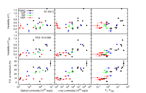
Figure 5.— Relations between measured properties. From the top to bottom, the distribution of variability of gamma-ray flux, that of optical flux, and maximum polarization are plotted with respect to optical luminosity, gamma-ray luminosity, and the ratio of latter to the former are plotted (from left to right). The black, blue, green, and red symbols indicate FSRQs, LSPs, ISPs, and HSPs, respectively.

Figure 6 shows the distribution of correlation coefficients between gamma-ray and optical luminosities, and between the optical luminosity and optical polarization degree. We used the DCF value with no time-lag for correlation coefficient (see Section 3.3). We find a weak correlation between the DCF value and the gamma-ray luminosity, similar to the case of gamma-ray luminosity vs. maximum polarization degree. The distribution of correlation between optical flux and optical polarization is similar to that reported in Paper I.

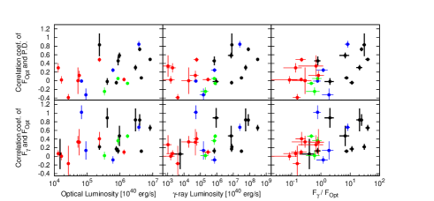
Figure 6.— Scatter plot of correlation coefficient and gamma-ray luminosity, optical luminosity and ratio of gamma-ray flux and optical flux. Top panels show DCF value corresponding to zero time lag between optical flux and optical polarization degree. Bottom panels show DCF value corresponding to zero time lag between gamma-ray flux and optical flux. Colors are the same as those of Figure 5.

4. Discussion

4.1. Summary of our observations

We collected a large amount of simultaneous gamma-ray and optical photopolarimetric data on the variability of blazars. We confirmed that basic properties, such as a relation between the synchrotron peak frequency and the amplitude of flux variability, are the same as reported in Paper I. Paper I suggested that blazars with the peak of the synchrotron radiation located at higher frequencies had smaller amplitude variations in the flux, color, and polarization degree. In addition, we found that some blazars show a significant correlation between the gamma-ray and optical fluxes, as well as between the optical flux and polarization degree (as seen in Bonning et al., 2009, 2012). In the case of correlation between gamma-ray and optical fluxes, about 15 out of 24 ($\sim$ 63%) objects show a significant correlation. In particular, 7 out of 11 FSRQ blazars and 8 out of 13 BL Lac objects show a strong correlation. This result is consistent with that reported in Hovatta et al. (2014). We also found a good relation between the correlation coefficient between gamma-ray and optical fluxes and the gamma-ray luminosity, as shown in Fig. 6. A similar relation was found for the correlation coefficient between the optical flux and optical polarization degree.

4.2. Systematic variation of the maximum polarization degree across blazar sequence

In this section, we discuss possible origin of the systematic trend in the maximum optical polarization degree that is increasing from the HSP ($\sim 10\%$) to the LSP ($\sim 40\%$) blazars. The maximum optical polarization degree as determined for individual sources appears to be fundamentally correlated with either the gamma-ray luminosity or with the Compton dominance (here represented by the ratio of gamma-ray to optical fluxes).

The optical emission of most blazars is dominated by synchrotron emission, but in some FSRQs in their low state can be contaminated by the thermal emission from the accretion disk (in our sample, this seems to be the case for 3C 273). The synchrotron emission of blazars observed in the optical band is optically thin. The linear polarization of the optically thin synchrotron radiation depends primarily on the structure of magnetic fields in the emitting region, and partially on the energy distribution of emitting electrons.

The polarization degree of synchrotron radiation is maximized for uniform magnetic fields, and it depends on the electron energy distribution index $p$ (such that $N(\gamma)\propto\gamma^{-p}$): $\Pi_{\rm max}=(p+1)/(p+7/3)$ (Westfold, 1959). However, since $\Pi_{\rm max}$ varies between 60% for $p$ = 1 and 80% for $p$ = 4, it is not possible to explain large systematic variations in the polarization degree solely by varying the electron distribution function.

Therefore, we need to consider scenarios in which the magnetic fields in the emitting regions of FSRQs are systematically better organized than in the case of BL Lacs. Magnetic fields can be expected to be well organized at the base of relativistic jets, where the magnetization parameter ($\sigma_{B}=\frac{B^{2}}{4\pi w}$, where $w$ is the specific enthalpy) is well above unity. As the jets evolve with distance, their magnetic energy is converted to kinetic energy, and they are thought to roughly approach equipartition. In this condition, it is likely that magnetic fields become tangled by turbulent plasma motions, e.g., triggered by current-driven instabilities (Begelman, 1998). If the chaotic magnetic field is completely isotropic, it will produce no net synchrotron polarization. However, as noted by Laing (1980), such chaotic fields can be compressed by shock waves, resulting in the polarization degree (Hughes et al., 1985):

$$\Pi_{\rm max}=\frac{(p+1)}{(p+7/3)}\;\frac{(1-k^{2})\cos^{2}\Phi^{\prime}}{[2-(1-k^{2})\cos^{2}\Phi^{\prime}]},$$ (3)

where $k$ is the shock compression ratio and $\Phi^{\prime}$ is the inclination of the observer to the shock compression plane in the downstream jet co-moving frame. For example, assuming $p=2$ and $\Phi^{\prime}=0$, the typical maximum polarization degree value for FSRQs ($\Pi_{\rm max}\simeq 0.4$) corresponds to $k\simeq 0.5$, and that for BL Lacs ($\Pi_{\rm max}\simeq 0.1$) corresponds to $k\simeq 0.9$. This would suggest very weak shock waves in the case of BL Lacs, potentially creating a problem for efficient particle acceleration. The distribution of viewing angles in the co-moving frame can be expected to be roughly isotropic, hence, it is very unlikely that the $\Pi_{\rm max}$ values could be reduced at low shock compression ratios due to a specific choice of $\Phi^{\prime}$ values. If there would be strong shock waves with very low compression ratios, we should observe even higher polarization degrees in some blazars. Therefore, we think that variations in the shock compression ratio cannot reasonably explain the differences in maximum polarization degree across different types of blazars.

Depolarization of synchrotron radiation could result from a superposition of multiple emitting regions with independent orientations of magnetic field lines (Jones et al., 1985). In such a case, BL Lacs should be characterized by a larger number of emitting regions. This would also predict a smaller variability index. In fact, our results indicate the optical variability index is correlated with the Compton dominance, but no such trend is apparent for the gamma-ray variability index (see Figure 5).

Such multiple emitting regions in blazars might be characterized by the distribution of electron energies varying from one region to another. The typical electron energy $\gamma_{\rm opt}\propto[(1+z)\nu_{\rm opt}/(\Gamma_{\rm j}B^{\prime})]^{1/2}$ corresponding to the optical band is somewhat higher in the case of BL Lacs than in FSRQs. This is because FSRQs show higher Lorentz factors $\Gamma_{\rm j}$ (Hovatta et al., 2009) and stronger magnetic fields $B^{\prime}$ (Pushkarev et al., 2012) than BL Lacs, although these differences are not large. However, the electron energy distribution extends to a significantly higher maximum characteristic energy $\gamma_{\rm max}\gg\gamma_{\rm opt}$ in the case of BL Lacs (where the synchrotron component extends to the X-ray band) than in the case of FSRQs (where $\gamma_{\rm max}\sim\gamma_{\rm opt}$). If the number of emitting regions or the volume filling factor scale with $\gamma/\gamma_{\rm max}$, this could explain a lower effective polarization degree of BL Lacs (e.g., Marscher & Jorstad, 2010). This predicts that the variability index scales with $\gamma/\gamma_{\rm max}$ , and indeed there is some observational evidence that this is the case (e.g., Aleksić et al., 2015). This also predicts a high X-ray polarization degree for BL Lac objects, which can be verified by future X-ray polarimetric missions.

A particular scenario that could explain our main result is a spine-sheath model (Ghisellini et al., 2005), in which the fast spine has ordered magnetic fields and the slow sheath has chaotic magnetic fields. In this scenario, the spine region would produce a highly variable and polarized synchrotron component, and the sheath region would produce a steady and weakly polarized component. In order to explain the systematic trend in maximum polarization degree, the jet volume fraction occupied by the spine should increase from the BL Lacs to the FSRQ blazars.

These scenarios should be related to the fundamental differences between the relativistic jets of FSRQs and BL Lacs. In the Unification Model for AGNs (Urry & Padovani, 1995), FSRQs are associated with powerful FR II radio galaxies (Fanaroff & Riley, 1974), and BL Lacs are associated with relatively weak FR I radio galaxies. FR II jets are known to form strong hotspots, which indicates that they carry a relatively large fraction of their initial kinetic power to distances $>100\;{\rm kpc}$. On the other hand, FR I jets appear to gradually dissipate their kinetic energy, so that they do not form hotspots. This suggests that FR I jets are more turbulent, and therefore their magnetic fields are more chaotic and less organized, than FR II jets (e.g., Tchekhovskoy & Bromberg, 2016). This fundamental dichotomy in the properties of relativistic jets naturally explains our observational result that the maximum optical polarization degree is systematically higher in the FSRQs as compared to the BL Lacs. However, most of the blazar emission is expected to be produced roughly on pc scales (e.g., Nalewajko et al., 2014), and hence this dichotomy (FRI or FRII) in jet properties should manifest itself already at these scales.

5. Conclusion

We performed long-term photopolarimetric monitoring of GeV bright blazars detected by the Fermi-LAT using Kanata telescope for 6.5 years. We selected 45 blazars of various sub-types, and obtained densely-sampled simultaneous light curves in the optical and GeV band for 24 blazars. Our results are (1) some blazars show a significant correlation between the gamma-ray and optical fluxes, as well as between the optical flux and polarization degree, (2) a significant correlation between the maximum degree of optical linear polarization and the gamma-ray luminosity. These relations are also confirmed with the ratio of gamma-ray to optical fluxes instead of gamma-ray luminosity. These results can be explained by a spine-sheath model and systematic difference in the intrinsic alignment of magnetic fields in relativistic jets (e.g., FSRQs vs. BL Lacs or FR Is vs. FR IIs). A measurement of flare amplitude and frequency could be related with size and number of emission regions in the jet, therefore such a measurement of “Flare cadence” will be helpful to test the assumptions of this model.

Appendix A

Figure 7.— Multiwavelength light curves of S2 0109+224. Details of plots are shown in Fig. 1. Non-simultaneous data are represented by open boxes. Upper limits on the gamma-ray flux are indicated by open triangles.

Figure 8.— Multiwavelength light curves of MisV 1436

Figure 9.— Multiwavelength light curves of 3C 66A

Figure 10.— Multiwavelength light curves of AO 0235+164

Figure 11.— Multiwavelength light curves of PKS 0454+234

Figure 12.— Multiwavelength light curves of S5 0716+714

Figure 13.— Multiwavelength light curves of OJ 49

Figure 14.— Multiwavelength light curves of OJ 287

Figure 15.— Multiwavelength light curves of Mrk 421

Figure 16.— Multiwavelength light curves of ON 325

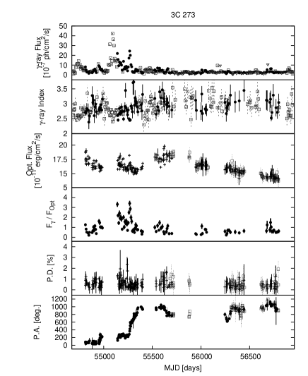
Figure 17.— Multiwavelength light curves of 3C 273

Figure 18.— Multiwavelength light curves of 3C 279

Figure 19.— Multiwavelength light curves of PKS 1502+106

Figure 20.— Multiwavelength light curves of PKS 1510-089

Figure 21.— Multiwavelength light curves of RX J1542.8+6129

Figure 22.— Multiwavelength light curves of PG 1553+113

Figure 23.— Multiwavelength light curves of Mrk 501

Figure 24.— Multiwavelength light curves of PKS 1749+096

Figure 25.— Multiwavelength light curves of 3C 371

Figure 26.— Multiwavelength light curves of 1ES 1959+650

Figure 27.— Multiwavelength light curves of PKS 2155-304

Figure 28.— Multiwavelength light curves of BL Lac

Figure 29.— Multiwavelength light curves of CTA 102

Figure 30.— Multiwavelength light curves of 3C 454.3

Appendix B

Basic block Bootstrap is a simulation method used to estimate the distribution of test statistics. It is used for time series data (e.g., Loh, 2008). The original dataset is split into $N_{\rm block}$ non-overlapping blocks. We then randomly resampled the dataset based on these blocks from the original data, and calculated the correlation coefficient between the original and the replacement data. This routine was repeated 10,000 times to obtain the Bootstrap distribution of correlation coefficient for each dataset. From this Bootstrap distribution, a confidence interval of $\alpha=0.95$ was derived. For blazars, the typical timescale of a flare is about a few weeks and the cadence of our dataset is typically a few days. Therefore, $N_{\rm block}\sim 5$ corresponds to the typical timescale of blazar flares. In this paper, we fixed the $N_{\rm block}$ = 5 for all of our samples. Of course, different blazars have different timescales but we also confirmed that the confidence interval dependence on block size is negligible. Table 6 summarizes the confidence level dependence on block size for the correlation coefficient of gamma-ray flux and optical flux with a time lag of zero for S5 0716+714.

Table 6Confidence interval dependence on block size

Block size ($N_{\rm block}$)	95% C.I.
3	(0.1852 0.4846)
4	(0.1871, 0.4847)
5	(0.1887, 0.4842)
6	(0.1903, 0.4824)
7	(0.1885, 0.4826)
8	(0.1869, 0.4842)
9	(0.1885, 0.4831)
10	(0.1894, 0.4828)
20	(0.1904, 0.4826)
30	(0.1891, 0.4845)
50	(0.1922, 0.4843)
100	(0.1960, 0.4881)

References

- Acero et al. (2015) Acero, F., Ackermann, M., Ajello, M., et al. 2015, ApJS, 218, 23
- Acero et al. (2016) Acero, F., Ackermann, M., Ajello, M., et al. 2016, ApJS, 223, 26
- Ackermann et al. (2011) Ackermann, M., Ajello, M., Allafort, A., et al. 2011, ApJ, 743, 171
- Ackermann et al. (2015a) Ackermann, M., Ajello, M., Albert, A., et al. 2015a, ApJ, 813, L41
- Ackermann et al. (2015b) Ackermann, M., Ajello, M., Atwood, W. B., et al. 2015b, ApJ, 810, 14
- Agudo et al. (2011) Agudo, I., Marscher, A. P., Jorstad, S. G., et al. 2011, ApJ, 735, L10
- Aleksić et al. (2015) Aleksić, J., Ansoldi, S., Antonelli, L. A., et al. 2015, A&A, 578, A22
- Atwood et al. (2009) Atwood, W. B., Abdo, A. A., Ackermann, M., et al. 2009, ApJ, 697, 1071
- Begelman (1998) Begelman, M. C. 1998, ApJ, 493, 291
- Blinov et al. (2015) Blinov, D., Pavlidou, V., Papadakis, I., et al. 2015, MNRAS, 453, 1669
- Bonning et al. (2012) Bonning, E., Urry, C. M., Bailyn, C., et al. 2012, ApJ, 756, 13
- Bonning et al. (2009) Bonning, E. W., Bailyn, C., Urry, C., et al. 2009, in American Astronomical Society Meeting Abstracts, Vol. 214, American Astronomical Society Meeting Abstracts 214, 686
- Brand (1985) Brand, P. W. J. L. 1985, Infrared and optical photopolarimetry of blazars, ed. T. Neckel & H. Vehrenberg, 215–219
- Edelson & Krolik (1988) Edelson, R. A., & Krolik, J. H. 1988, ApJ, 333, 646
- Fanaroff & Riley (1974) Fanaroff, B. L., & Riley, J. M. 1974, MNRAS, 167, 31P
- Finke (2013) Finke, J. D. 2013, ApJ, 763, 134
- Fossati et al. (1998) Fossati, G., Maraschi, L., Celotti, A., et al. 1998, MNRAS, 299, 433
- Ghisellini et al. (1998) Ghisellini, G., Celotti, A., Fossati, G., et al. 1998, MNRAS, 301, 451
- Ghisellini et al. (2005) Ghisellini, G., Tavecchio, F., & Chiaberge, M. 2005, A&A, 432, 401
- Hovatta et al. (2009) Hovatta, T., Valtaoja, E., Tornikoski, M., et al. 2009, A&A, 494, 527
- Hovatta et al. (2014) Hovatta, T., Pavlidou, V., King, O. G., et al. 2014, MNRAS, 439, 690
- Hughes et al. (1985) Hughes, P. A., Aller, H. D., & Aller, M. F. 1985, ApJ, 298, 301
- Ikejiri et al. (2011) Ikejiri, Y., Uemura, M., Sasada, M., et al. 2011, PASJ, 63, 639
- Janiak et al. (2012) Janiak, M., Sikora, M., Nalewajko, K., et al. 2012, ApJ, 760, 129
- Jones et al. (1985) Jones, T. W., Rudnick, L., Fiedler, R. L., Aller, H. D., Aller, M. F., & Hodge, P. E., 1985, ApJ, 290, 627
- Kawabata et al. (2008) Kawabata, K. S., Nagae, O., Chiyonobu, S., et al. 2008, in Society of Photo-Optical Instrumentation Engineers (SPIE) Conference Series, Vol. 7014, Society of Photo-Optical Instrumentation Engineers (SPIE) Conference Series
- Kiehlmann et al. (2016) Kiehlmann, S., Savolainen, T., Jorstad, S. G., et al. 2016, A&A, 590, A10
- Laing (1980) Laing, R. A. 1980, MNRAS, 193, 439
- Loh (2008) Loh, J. M. 2008, ApJ, 681, 726
- Marscher & Jorstad (2010) Marscher, A. P., & Jorstad, S. G. 2010, ArXiv e-prints
- Marscher et al. (2008) Marscher, A. P., Jorstad, S. G., D’Arcangelo, F. D., et al. 2008, Nature, 452, 966
- Mead et al. (1990) Mead, A. R. G., Ballard, K. R., Brand, P. W. J. L., Hough, J. H., Brindle, C., & Bailey, J. A. 1990, A&AS, 83, 183
- Nalewajko et al. (2014) Nalewajko, K., Begelman, M. C., & Sikora, M. 2014, ApJ, 789, 161
- Nalewajko et al. (2012) Nalewajko, K., Sikora, M., Madejski, G. M., Exter, K., Szostek, A., Szczerba, R., Kidger, M. R., & Lorente, R. 2012, ApJ, 760, 69
- Nandra et al. (1997) Nandra, K., George, I. M., Mushotzky, R. F., Turner, T. J., & Yaqoob, T. 1997, ApJ, 476, 70
- Nilsson et al. (1999) Nilsson, K., Pursimo, T., Takalo, L. O., et al. 1999, PASP, 111, 1223
- Pushkarev et al. (2012) Pushkarev, A. B., Hovatta, T., Kovalev, Y. Y., Lister, M. L., Lobanov, A. P., Savolainen, T., & Zensus, J. A. 2012, A&A, 545, A113
- Sasada et al. (2008) Sasada, M., Uemura, M., Arai, A., et al. 2008, PASJ, 60, L37
- Schulz & Lenzen (1983) Schulz, A., & Lenzen, R. 1983, A&A, 121, 158
- Stickel et al. (1991) Stickel, M., Padovani, P., Urry, C. M., Fried, J. W., & Kuehr, H. 1991, ApJ, 374, 431
- Tchekhovskoy & Bromberg (2016) Tchekhovskoy, A., & Bromberg, O. 2016, MNRAS, 461, L46
- Uemura et al. (2010) Uemura, M., Kawabata, K. S., Sasada, M., et al. 2010, PASJ, 62, 69
- Urry & Padovani (1995) Urry, C. M., & Padovani, P. 1995, PASP, 107, 803
- Visvanathan & Wills (1998) Visvanathan, N., & Wills, B. J. 1998, AJ, 116, 2119
- Watanabe et al. (2005) Watanabe, M., Nakaya, H., Yamamuro, T., et al. 2005, PASP, 117, 870
- Westfold (1959) Westfold, K. C. 1959, ApJ, 130, 241
- Wolff et al. (1996) Wolff, M. J., Nordsieck, K. H., & Nook, M. A. 1996, AJ, 111, 856