Post Selection Inference with Kernels

Abstract

We propose a novel kernel based post selection inference (PSI) algorithm, which can not only handle non-linearity in data but also structured output such as multi-dimensional and multi-label outputs. Specifically, we develop a PSI algorithm for independence measures, and propose the Hilbert-Schmidt Independence Criterion (HSIC) based PSI algorithm (hsicInf). The novelty of the proposed algorithm is that it can handle non-linearity and/or structured data through kernels. Namely, the proposed algorithm can be used for wider range of applications including nonlinear multi-class classification and multi-variate regressions, while existing PSI algorithms cannot handle them. Through synthetic experiments, we show that the proposed approach can find a set of statistically significant features for both regression and classification problems. Moreover, we apply the hsicInf algorithm to a real-world data, and show that hsicInf can successfully identify important features.

1 Introduction

Finding a set of features in high-dimensional data is an important problem with many real-world problems such as biomarker discovery (Xing et al., 2001), document categorization (Forman, 2008), and prosthesis control (Shenoy et al., 2008), to name a few. In particular, finding a set of statistically significant features is crucial for scientific discovery, and linear methods including the least absolute shrinkage and selection operator (LASSO) (Tibshirani, 1996) are extensively used. However, LASSO focuses on finding a set of linearly related features. Thus, if an input and output pair has non-linear relationship, it is hard to find a set of important features.

To select non-linearly related features, a feature screening approach, which is based on ranking features with respect to the association score between each feature and its output, is widely used (Fan and Lv, 2008). Typically, the correlation coefficient (linear) and the mutual information (non-linear) are used as an association measure (Cover and Thomas, 2006). Recently, the kernel based independence measure such as the Hilbert-Schmidt Independence Criterion (HSIC) (Gretton et al., 2005) and its normalized variant (NOCCO) were proposed and have started being used as a surrogate of the mutual information (Song et al., 2012; Balasubramanian et al., 2013; Fukumizu et al., 2008). The key advantage of the kernel based approaches is that it can deal with non-linearity and/or non-structured data including multi-variate and graph data through kernels. Besides association approaches, sparse regularization based approaches including the sparse additive model (SpAM) (Ravikumar et al., 2009) and HSIC LASSO (Yamada et al., 2014) are widely used in feature selection communities. These kernel based approaches are promising, however, it is not clear whether the selected features are statistically significant. Since the selection event needs to be taken into account for statistical inference, a naive two-step approach, which first selects features and then test the selected features without any adjustment, does not control the desired false positive rates.

The problem of testing the significance of the selected features is known as selective inference (Taylor and Tibshirani, 2015; Hastie et al., 2015). The data splitting approach is a typical selective inference algorithm. The key idea of the splitting approach is to divide a training dataset into two disjoint sets, and then, one of the sets is used for feature selection and the other is used for statistical inference. Since the selection event and the statistical inference are independent, we can successfully identify a set of statistically important features. However, since we divide a dataset into two disjoint sets and used them for feature selection and statistical inference, respectively, the detection power can be degraded.

Recently, a novel selective inference approach called the post selection inference (PSI) has been proposed (Hastie et al., 2015; Lockhart et al., 2014; Lee et al., 2016). PSI algorithms tend to have higher detection power than data splitting approaches. However, only linear approaches which are built upon LASSO or other similar linear feature selection approaches are available so far. Since real-world datasets tend to have non-linear relationship, the existing linear approaches may fail to find a set of important features; this is a critical problem in practice. Moreover, existing PSI approaches are only applicable to uni-variate output. Thus, the applications of existing PSI methods is limited.

In this paper, we propose a kernel based PSI method hsicInf, which can find statistically significant features from non-linear and/or structured output data such as multi-dimensional output. Specifically, we develop a PSI algorithm for independence measures, and propose the HSIC based PSI algorithm. A clear advantage of hsicInf over existing approaches is that it can easily handle non-linearity and structured data through kernels. Namely, it can be used for wider range of applications including multi-class classification and multi-variate regression. Through synthetic and real-world experiments, we show that the proposed approach can find a set of statistically significant features for both regression and classification problems.

Contribution:

• We propose a kernel based PSI algorithm that can handle non-linearity, multi-label, multi-class, and structured output. To the best of our knowledge, this paper presents the first kernel based PSI algorithm.

• We empirically show that the proposed algorithm can successfully identify a set of non-linearly related features.

2 Proposed method

In this section, we propose a PSI method with kernels. More specifically, we develop a new PSI framework based on an independence measure called the Hilbert-Schmidt Independence Criterion (HSIC) (Gretton et al., 2005; Zhang et al., 2016).

2.1 Problem Formulation

Let us denote an input vector by ${\bm{x}}=[x^{(1)},\dots,x^{(d)}]^{\top}\in\mathbb{R}^{d}$ and the corresponding target vector ${\bm{y}}\in\mathbb{R}^{d_{y}}$. i.i.d. samples $\{({\bm{x}}_{i},{\bm{y}}_{i})\}_{i=1}^{n}$ have been drawn from a joint probability density $p({\bm{x}},{\bm{y}})$. The final goal of this paper is to first screen $k<d$ features of input vector ${\bm{x}}$ and then test whether the selected features are of statistically significant association to its output ${\bm{y}}$.

2.2 Marginal screening and post-selection inference with independence measure

In this paper, we employ an estimate of the independence measure $\widehat{I}(X_{m},Y)$, which measures the discrepancy from the independence between the $m$-th random variable $X_{m}$ and its output variable $Y$, where the vector of independence measures denoted by ${\bm{z}}=[\widehat{I}(X_{1},Y),\ldots,\widehat{I}(X_{d},Y)]^{\top}$ follows a multi-variate normal distribution with ${\bm{\mu}}\in\mathbb{R}^{d}$ and ${\bm{\Sigma}}\in\mathbb{R}^{d\times d}$:

$${\bm{z}}\sim N({\bm{\mu}},{\bm{\Sigma}}).$$

Then, we exploit the normality of ${\bm{z}}$ and combine it with the post selection inference framework recently developed by (Lee et al., 2016) (see Theorem 1).

Theorem 1

(Lee et al., 2016). Consider a stochastic data generating process ${\bm{{\mathcal{Z}}}}\sim N({\bm{\mu}},{\bm{\Sigma}})$. If a feature selection event is characterized by ${\bm{A}}{\bm{{\mathcal{Z}}}}\leq{\bm{b}}$ for a matrix ${\bm{A}}$ and a vector ${\bm{b}}$ that do not depend on ${\bm{{\mathcal{Z}}}}$, then, for any fixed vector ${\bm{\eta}}\in\mathbb{R}^{d}$,

$$F^{[V^{-}({\bm{A}},{\bm{b}}),V^{+}({\bm{A}},{\bm{b}})]}_{{\bm{\eta}}^{\top}{\bm{\mu}},{\bm{\eta}}^{\top}{\bm{\Sigma}}{\bm{\eta}}}({\bm{\eta}}^{\top}{\bm{{\mathcal{Z}}}})~{}~{}|~{}~{}{\bm{A}}{\bm{{\mathcal{Z}}}}\leq{\bm{b}}\sim\textnormal{Unif}(0,1),$$

where $F^{[v,w]}_{t,u}(\cdot)$ is the cumulative distribution function of the uni-variate truncated normal distribution with the mean $t$, the variance u, and the lower and the upper truncation points $v$ and $w$, respectively. Furthermore, using ${\bm{c}}:=\frac{{\bm{\Sigma}}{\bm{\eta}}}{{\bm{\eta}}^{\top}{\bm{\Sigma}}{\bm{\eta}}}$, the lower and the upper truncation points are given as

$$V^{-}({\bm{A}},{\bm{b}}) :=\max_{j:({\bm{A}}{\bm{c}})_{j}<0}\left\{\frac{b_{j}-({\bm{A}}{\bm{z}})_{j}}{({\bm{A}}{\bm{c}})_{j}}\right\}+{\bm{\eta}}^{\top}{\bm{z}},$$ (1)

$$V^{+}({\bm{A}},{\bm{b}}) :=\min_{j:({\bm{A}}{\bm{c}})_{j}>0}\left\{\frac{b_{j}-({\bm{A}}{\bm{z}})_{j}}{({\bm{A}}{\bm{c}})_{j}}\right\}+{\bm{\eta}}^{\top}{\bm{z}}.$$ (2)

$\Box$

In order to develop post selection inference method for the independence measure ${\bm{z}}$, we confirm that the problem of selecting top $k$ features in the decreasing order of $\widehat{I}(X_{\cdot},Y)$ can be represented as a linear selection event in the form of ${\bm{A}}{\bm{z}}\leq{\bm{b}}$ in Theorem 1.

We denote the index set of the selected $k$ features by ${\mathcal{S}}$, and that of the unselected $\bar{k}=d-k$ features by $\bar{{\mathcal{S}}}$. The fact that $k$ features in ${\mathcal{S}}$ are selected and $\bar{k}$ features in $\bar{{\mathcal{S}}}$ are not selected is rephrased by

$$\widehat{I}(X_{m},Y)\geq\widehat{I}(X_{\ell},Y),~{}~{}\text{for all}~{}(m,\ell)\in{\mathcal{S}}\times\bar{{\mathcal{S}}}.$$ (3)

Here, we have in total $k\bar{k}$ constraints written as the linear inequalities with respect to ${\bm{z}}$. Furthermore, the truncation points in Theorem 1 can be explicitly stated as follows.

Theorem 2

Let $\theta\in[k\bar{k}]$ be the index of the first $k\bar{k}$ affine constraints in Eq. (3) and $C:=\{1,\ldots,k\bar{k}\}$. Furthermore, for notational simplicity, assume that first $k$ features are selected and remaining $\bar{k}=d-k$ features are unselected. Then, the marginal screening event in Eq. (3) is written as

$$({\bm{A}}{\bm{z}})_{\theta}=\widehat{{I}}(X_{\ell(\theta)},Y)-\widehat{{I}}(X_{m(\theta)},Y)\leq 0$$

$$~{}\text{with}~{}m(\theta):=\left\lceil\theta/\bar{k}\right\rceil,\ell(\theta):=k+(\theta~{}\textnormal{mod}~{}\bar{k})~{}\theta\in C.$$

The lower and the upper truncation points for $m$-th feature are written as

$$V^{-}({\bm{A}},{\bm{0}})$$

$$\!:=\!\max_{\theta\in{\mathcal{D}}}\!\left\{\!\frac{\![{\bm{\Sigma}}]_{m,m}\!\!\left(\!\widehat{{I}}(X_{m(\theta)},Y)\!-\!\widehat{{I}}(X_{\ell(\theta)},Y)\!\right)\!}{[{\bm{\Sigma}}]_{\ell(\theta),m}-[{\bm{\Sigma}}]_{m(\theta),m}}\!\right\}\!\!+\!\widehat{{I}}(X_{m},Y),$$

$$V^{+}({\bm{A}},{\bm{0}})$$

$$\!:=\!\min_{\theta\in\bar{{\mathcal{D}}}}\!\left\{\!\frac{\![{\bm{\Sigma}}]_{m,m}\!\!\left(\!\widehat{{I}}(X_{m(\theta)},Y)\!-\!\widehat{{I}}(X_{\ell(\theta)},Y)\!\right)\!}{[{\bm{\Sigma}}]_{\ell(\theta),m}-[{\bm{\Sigma}}]_{m(\theta),m}}\!\right\}\!\!+\!\widehat{{I}}(X_{m},Y),$$

where

$${\mathcal{D}} =\{\theta~{}~{}|~{}~{}[{\bm{\Sigma}}]_{\ell(\theta),m}<[{\bm{\Sigma}}]_{m(\theta),m}\},$$

$$\bar{{\mathcal{D}}} =\{\theta~{}~{}|~{}~{}[{\bm{\Sigma}}]_{\ell(\theta),m}>[{\bm{\Sigma}}]_{m(\theta),m}\}.$$

Proof: For deriving the lower and upper bounds, we simply need to plug ${\bm{\eta}}={\bm{e}}_{m}$ (the unit vector whose $m$-th element is one and zero otherwise), ${\bm{b}}={\bm{0}}$, $-({\bm{A}}{\bm{z}})_{\theta}=\widehat{I}(X_{m(\theta)},Y)-\widehat{I}(X_{\ell(\theta)},Y)$, and $({\bm{A}}{\bm{c}})_{\theta}=\left[\frac{[{\bm{\Sigma}}]_{\ell(\theta),m}-[{\bm{\Sigma}}]_{m(\theta),m}}{[{\bm{\Sigma}}]_{m,m}}\right]$ into Eq.  (1) and Eq. (2). $\Box$

2.3 HSIC based Post Selection Inference (hsicInf)

Here, we propose the Hilbert-Schmidt Independence Criterion (HSIC) (Gretton et al., 2005) based PSI algorithm.

Hilbert-Schmidt Independence Criterion (HSIC)

HSIC is defined as (Gretton et al., 2005):

$$\textnormal{HSIC}(X,Y) \!=\!\mathbb{E}_{{\bm{x}},{\bm{x}}^{\prime},{\bm{y}},{\bm{y}}^{\prime}}[K({\bm{x}},{\bm{x}}^{\prime})L({\bm{y}},{\bm{y}}^{\prime})]$$

$$\phantom{=}+\mathbb{E}_{{\bm{x}},{\bm{x}}^{\prime}}[K({\bm{x}},{\bm{x}}^{\prime})]\mathbb{E}_{{\bm{y}},{\bm{y}}^{\prime}}[L({\bm{y}},{\bm{y}}^{\prime})]$$ (4)

$$\phantom{=}-2\mathbb{E}_{{\bm{x}},{\bm{y}}}\left[\mathbb{E}_{{\bm{x}}^{\prime}}[K({\bm{x}},{\bm{x}}^{\prime})]\mathbb{E}_{{\bm{y}}^{\prime}}[L({\bm{y}},{\bm{y}}^{\prime})]\right],$$

where $K({\bm{x}},{\bm{x}}^{\prime})$ and $L({\bm{y}},{\bm{y}}^{\prime})$ are unique positive definite kernel, and $\mathbb{E}_{{\bm{x}},{\bm{x}}^{\prime},{\bm{y}},{\bm{y}}^{\prime}}$ denotes the expectation over independent pairs $({\bm{x}},{\bm{y}})$ and $({\bm{x}}^{\prime},{\bm{y}}^{\prime})$ drawn from $p({\bm{x}},{\bm{y}})$. With the use of characteristic kernels (Fukumizu et al., 2004; Sriperumbudur et al., 2011), HSIC takes zero if $X$ and $Y$ are independent, and takes positive values otherwise. Thus, we can select important features by ranking HSIC scores $\{\textnormal{HSIC}(X_{m},Y)\}_{m=1}^{d}$ in descending order, where $X_{m}$ is the random variable of the $m$-th feature.

Empirical Block Hilbert-Schmidt Independence Criterion (HSIC)

Let us assume that the number of samples $n$ can be dis-jointly divided into $\frac{n}{B}$ blocks, where $B$ is the number of samples in each block. Then, the disjoint set of blocked paired samples is denoted by $\{\{({\bm{x}}_{i}^{(b)},{\bm{y}}_{i}^{(b)})\}_{i=1}^{B}\}_{b=1}^{n/B}$.

An empirical estimate of the unbiased block HSIC is given by (Zhang et al., 2016)

$$\widehat{\text{HSIC}}(X,Y)=\frac{B}{n}\sum_{b=1}^{n/B}\widehat{\eta}_{b},$$

$$\widehat{\eta}_{b}=\frac{1}{B(B-3)}[\text{tr}(\bar{{\bm{K}}}^{(b)}\bar{{\bm{L}}}^{(b)})+\frac{{\bm{1}}_{B}^{\top}\bar{{\bm{K}}}^{(b)}{\bm{1}}_{B}{\bm{1}}_{B}^{\top}\bar{{\bm{L}}}^{(b)}{\bm{1}}_{B}}{(B-1)(B-2)}$$

$$\phantom{\widehat{\eta}_{b}=}-\frac{2}{B-2}{\bm{1}}_{B}^{\top}\bar{{\bm{K}}}^{(b)}\bar{{\bm{L}}}^{(b)}{\bm{1}}_{B}],$$

where ${\bm{K}}^{(b)}\in\mathbb{R}^{B\times B}$ is the input Gram matrix, ${\bm{L}}^{(b)}\in\mathbb{R}^{B\times B}$ is the output Gram matrix, $[\bar{{\bm{K}}}^{(b)}]_{ij}=[{\bm{K}}^{(b)}]_{ij}-\delta_{ij}[{\bm{K}}^{(b)}]_{ij}$ and $[\bar{{\bm{L}}}^{(b)}]_{ij}=[{\bm{L}}^{(b)}]_{ij}-\delta_{ij}[{\bm{L}}^{(b)}]_{ij}$, $\delta_{ij}$ takes 1 when $i=j$ and 0 otherwise, and ${\bm{1}}_{B}\in\mathbb{R}^{B}$ is the vector whose elements are all one. Since $\widehat{\eta}_{b}$ is computed from a partition of i.i.d. samples from $p({\bm{x}},{\bm{y}})$, $\{\widehat{\eta}_{b}\}_{b=1}^{n/B}$ is also an i.i.d. random variables.

The empirical block HSIC score asymptotically follows normal distribution when $B$ is finite and $n$ goes to infinity, and thus, we can use the block HSIC for PSI based on Theorem 2. Note that, to ensure Gaussian assumption, we need to have relatively large number of samples $n$ with a finite block size $B$.

Choice of Kernel: For regression problems, we use the Gaussian kernel for both input and output as ${\bm{K}}^{(b)}\in\mathbb{R}^{B\times B}$ and ${\bm{L}}^{(b)}\in\mathbb{R}^{B\times B}$:

$$[{\bm{K}}^{(b)}]_{ij} =\exp\left(-\frac{\|{\bm{x}}_{i}^{(b)}-{\bm{x}}_{j}^{(b)}\|^{2}_{2}}{2\tau_{x}^{2}}\right),$$

$$[{\bm{L}}^{(b)}]_{ij} =\exp\left(-\frac{\|{\bm{y}}_{i}^{(b)}-{\bm{y}}_{j}^{(b)}\|^{2}_{2}}{2\tau_{y}^{2}}\right),$$

where $\tau_{x}>0$ and $\tau_{y}>0$ are kernel parameters.

For $L$-class classification problems (i.e., $y\in\{1,2,\ldots,L\}$), we can first transform the target vector $y=\ell$ as

$${\bm{y}}_{j} =[{0~{}\cdots 0~{}\underbrace{1}_{\ell}~{}0~{}\cdots 0}]^{\top}\in\mathbb{R}^{L},$$

and use the linear kernel:

$$[{\bm{L}}^{(b)}]_{ij}={\bm{y}}_{i}^{\top}{\bm{y}}_{j}=\left\{\begin{array}[]{cc}1&(y_{i}=y_{j})\\ 0&\textnormal{Otherwise}\end{array}\right..$$

Note that, this is equivalent to the delta kernel (Song et al., 2012).

Mean and covariance matrix estimation: Suppose that the mean and variance of the within-block estimator $\widehat{\eta}_{b}$ are $\widetilde{\mu}$ and $\widetilde{\sigma}$, respectively. Then, the vector of empirical HSICs $[\widehat{\textnormal{HSIC}}(X_{1},Y),\ldots,\widehat{\textnormal{HSIC}}(X_{d},Y)]^{\top}\in\mathbb{R}^{d}$ converges in distribution to a multi-variate normal by the central limit theorem, where the mean and covariance matrices are given by by $\widetilde{\mu}$ and $n/B\widetilde{\sigma}$, respectively. In estimating $[\widetilde{{\bm{\Sigma}}}]_{m,m^{\prime}}$, the standard covariance estimator is applied to the ($n/B$) within-block estimators for $m$ and $m^{\prime}$. Note that, when $n/B$ is too small, we can use a high-dimensional covariance estimation algorithm such as POET (Fan et al., 2013).

Post Selection Inference: We consider the following hypothesis tests:

• $H_{0,m}$: $\textnormal{HSIC}(X_{m},Y)=0~{}|~{}\text{${\mathcal{S}}$ was selected}$,

• $H_{1,m}$: $\textnormal{HSIC}(X_{m},Y)~{}\neq 0~{}|~{}\text{${\mathcal{S}}$ was selected}$.

Then, the $p$-value of the $m$-th feature is estimated by using Theorem 2.

3 Related Work

In this section, we briefly review related works. It has long been recognized that selection bias must be corrected for statistical inference after feature selection. In machine learning community, the most common approach for dealing with selection bias is data splitting. In data splitting, the dataset is divided into two disjoint sets, and one of them is used for feature selection, and the other is used for statistical inference. Since the inference phase is made independently of the feature selection phase, we do not have to care about the selection effect. An obvious drawback of data splitting is that the powers are low both in feature selection and inference phases. Since only a part of the dataset can be used in feature selection phase, the risk of failing to select truly important features would increase. Similarly, the power of statistical inference (i.e., the probability of true positive finding) would decrease because the inference is made with a smaller dataset. In addition, it is quite annoying that different features might be selected if the dataset is divided differently. It is important to note that data splitting is also regarded as a selective inference because the inference is made only for the selected features in the feature selection phase, and the other unselected features are ignored.

In statistics, simultaneous inference has been studied traditionally for selection bias correction. For feature selection bias correction, all possible subsets of features are considered. Let $\widehat{\cal S}$ represent the set of selected features and $T_{j}({\cal S})$ be a test statistic for the $j^{\rm th}$ selected feature in $\widehat{\cal S}$. In simultaneous inference, critical points $l$ and $u$ at level $\alpha$ are determined to satisfy

$$P(T_{j}(\widehat{\cal S})\notin[l,u]\text{ for any subset of features $\widehat{\cal S}$})\leq\alpha.$$ (6)

The probability in (6) is also written as

$$P(T_{j}(\widehat{\cal S})\notin[l,u]\text{ for any subset of features $\widehat{\cal S}$})$$

$$=\sum_{{\cal S}}P(T_{j}(\widehat{\cal S})\notin[l,u]\mid\widehat{\cal S}={\cal S})P(\widehat{\cal S}={\cal S}),$$

where the summation in the right hand side runs over all possible subsets of features. Unfortunately, unless the number of original features is fairly small, it is computationally challenging to consider all possible subsets of features $\widehat{{\cal S}}$ (Berk et al., 2013).

In selective inference, we only consider the case that a certain $\cal S$ is selected, and we determine the critical points $l$ and $u$ so that selective type I error is controlled, i.e.,

$$P(T_{j}(\widehat{\cal S})\notin[l,u]\mid\widehat{\cal S}={\cal S})\leq\alpha.$$ (7)

Selective inference framework in the form of (7) has been increasingly popular after the seminal work by Lee et al. (2016). In this work, the authors studied selective inference after a subset of features are selected by LASSO (Tibshirani, 1996). Their novel finding is that, in linear regression models with Gaussian noise, if the selection event can be represented by a set of linear inequalities with respect to the response variables (as in LASSO case), then any linear combination of the responses conditioned on the selection event is distributed according to some truncated normal distribution as discussed in Theorem 1. This seminal result is known as a polyhedral lemma and is very useful for deriving a null distribution of a test statistic in the context of selective inference. After this work, selective inference framework has been studied for several problems where the assumptions of polyhedral lemma are satisfied (see, e.g., (Lee and Taylor, 2014)).

Unfortunately, polyhedral lemma in (Lee et al., 2016) can be used only when the responses are normally distributed. It is thus difficult to generalize selective inference framework to other important problem such as classification, multi-task learning and so on. To the best of our knowledge, there are only a few attempts of selective inference in those generalized settings (Taylor and Tibshirani, 2016). The idea in these attempts is to use asymptotic theory, but the underlying assumption used in these studies is somewhat restrictive. Specifically, they require that at least one truncation points are bounded in probability tending to 1, which is somewhat embarrassing because the truncation points are not bounded in the case of classical inference without feature selection. In contrast, our proposed method is not suffered from such a restriction because we only use an asymptotic normality of $\widehat{\rm HSIC}(X_{j},Y)$. In our method, since the test is conducted within the reproducing kernel Hilbert space, selective inference is possible for a variety of response types that includes classification, ranking, or more generally, any structures responses.

4 Experiment

In this section, we evaluate the proposed algorithm in regression and classification problems.

4.1 Setup

We compared the performance of the proposed methods with the linear PSI method based on the least angle regression (Lee et al., 2016; Efron et al., 2004), which is a state-of-the-art PSI algorithm. In this paper, we used the larInf function in the R package selectiveInference. Moreover, we compared the proposed method with hsic, which first selects features by empirical HSIC and then test each HSIC score without adjusting the sampling distribution (i.e., $V^{-}({\bm{A}},{\bm{0}})=-\infty$ and $V^{+}({\bm{A}},{\bm{0}})=\infty$), and the data-splitting approach (split). For both proposed and the existing methods, we set the number of selected features as $k=10$ and the significance level $\alpha=0.05$. For HSIC based approaches, we used the block parameter $B=\{5,10\}$.

In PSI frameworks, the covariance matrix ${\bm{\Sigma}}$ is assumed to be known. However, since the true covariane matrix is not available in practice, we need to estimate the covariance matrix from data. To this end, for hsicInf and hsic, we divided the samples into two disjoint sets; we used $\frac{n}{3}$ samples for estimating ${\bm{\Sigma}}$ and the rest of $\frac{2n}{3}$ samples for selecting features and computing HSIC. For split, we divided the samples into three disjoint sets with sample size $\frac{n}{3}$. Then, we used each of them for estimating ${\bm{\Sigma}}$, selecting and testing features, and computing HSIC, respectively. In this paper, we employed the POET algorithm for the covariance matrix estimation (Fan et al., 2013).

In regression setup, the kernel parameters are experimentally set to $(\tau_{x},\tau_{y})=(1.0,1.0)$ for uni-variate setup and $(\tau_{x},\tau_{y})=(1.0,\textnormal{med}(\{\|{\bm{y}}_{i}-{\bm{y}}_{j}\|_{2}\}_{i,j=1}^{n}))$ for multi-variate output, respectively, where each feature was normalized to have mean zero and standard deviation 1. In classification setup, we used the Gaussian kernel for input and the delta kernel for output. We reported the true positive rate (TPR) $\frac{k^{\prime}}{k^{*}}$ where $k^{\prime}$ is the number of truely relevant features that are reported to be positive, while $k^{*}$ is the number of truly relevant features. We further computed the false positive rate (FPR) $\frac{k^{\prime\prime}}{k}$ where $k^{\prime\prime}$ is the number of truely irelevant features that are falsely reported to be positive.

4.2 False positive rate control

First, to check whether the methods can properly control the desired FPR, we run the proposed methods using a dataset that has no relationship between input and output. Specifically, we generated the input output pairs as $\{({\bm{x}}_{i},y_{i})\}_{i=1}^{n}$, where ${\bm{x}}\sim N({\bm{0}},{\bm{I}}_{20})$, ${\bm{0}}\in\mathbb{R}$ is the vector whose elements are all zero, ${\bm{I}}\in\mathbb{R}^{20\times 20}$ is the identity matrix, and $y\sim N(0,1)$.

Figure 1(a) shows that the FPRs of hsicInf, hsic, and split algorithms, respectively. The both the proposed method and split successfully control FPR, while hsic fails to control FPR. Thus, the adjustment of the sampling distribution is critical for estimating proper $p$-values. It shows that all FPRs tend to be high when the number of samples are small, and gradually converging to the significance level when the number of samples increases. Figures 1(b) shows the FPRs for the hsicInf algorithms with different block size $B$.

Since hsic cannot control the FPR at the desired level, we do not compare the TPR of hsic in the following section.

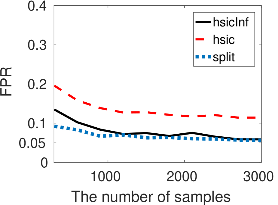
(a)

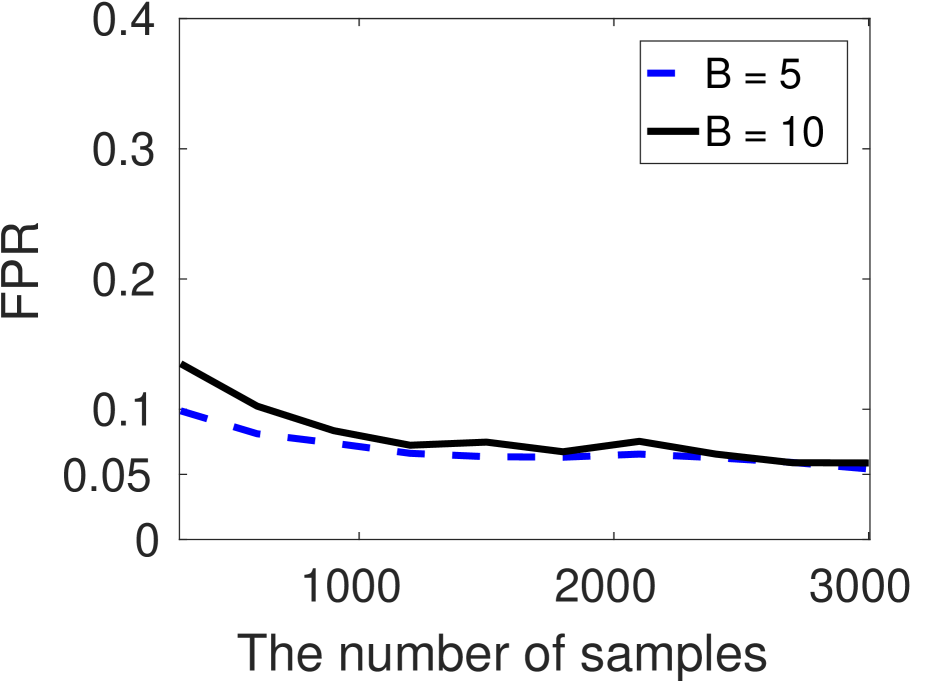
(b)

Figure 1: False positive rates at significant level $\alpha=0.05$ of the proposed methods. (a): Comparison of hsicInf, hsic, split, and larInf. We used $B=10$. (b): FPRs for hsicInf with different block parameter $B$. The hsic computes $p$-values without adjusting the sampling distribution by Theorem 2.

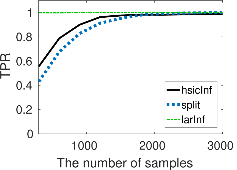
(a) Linear.

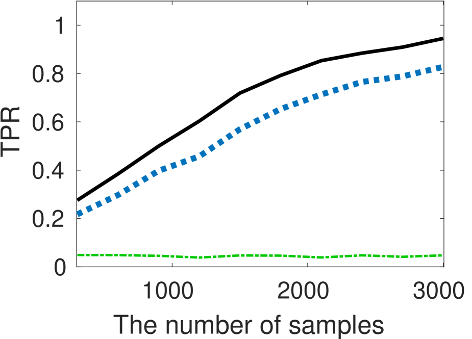
(b) Additive Non-linear.

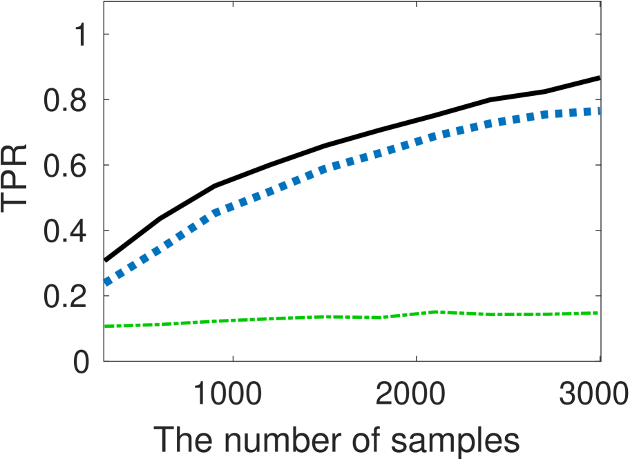
(c) Non-additive Non-linear.

(d) Linear.

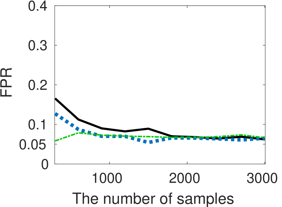
(e) Additive Non-linear.

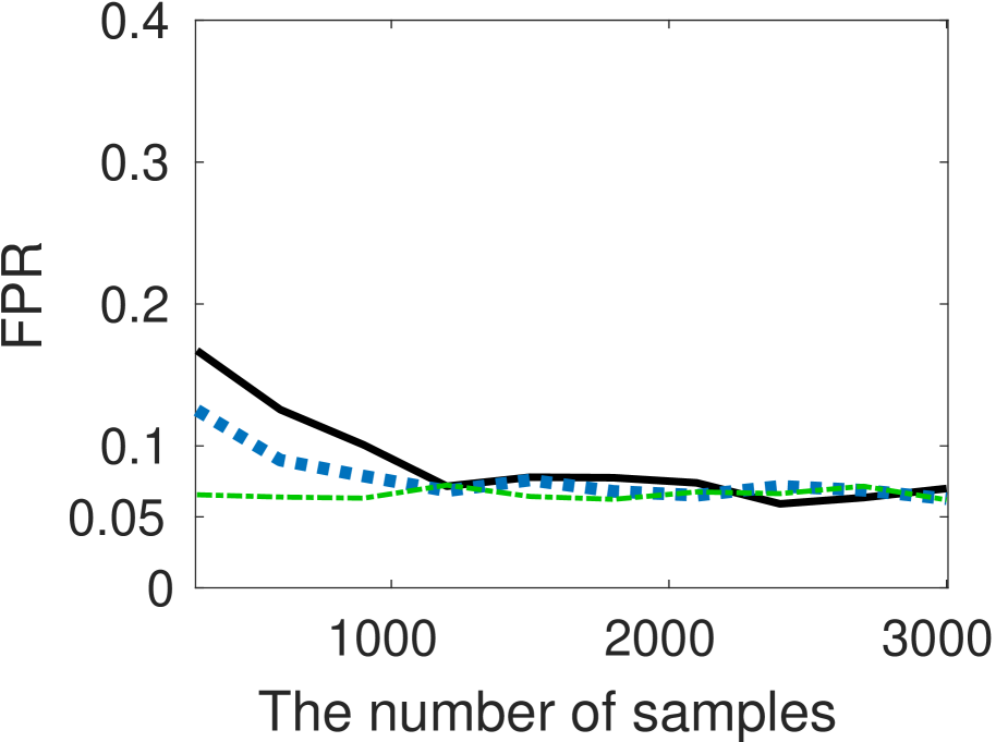
(f) Non-additive Non-linear.

Figure 2: The results for the uni-variate setups. We used $B=10$ for the hsic related methods. (a)-(c): TPRs. (d)-(f): FPRs.

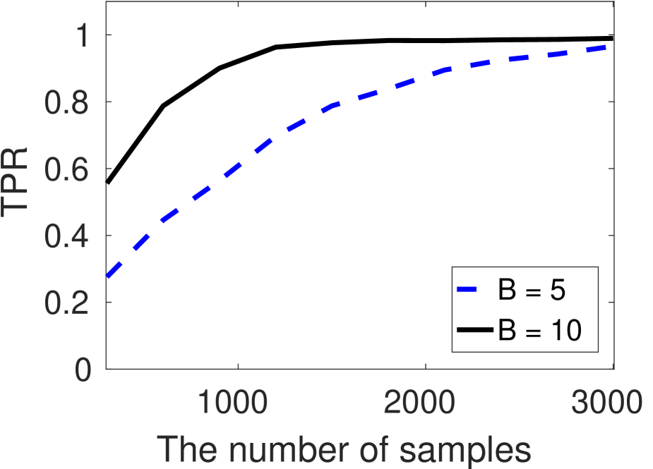
(a) Linear.

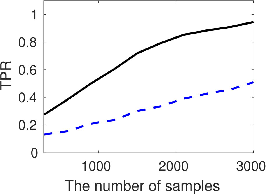
(b) Additive Non-linear.

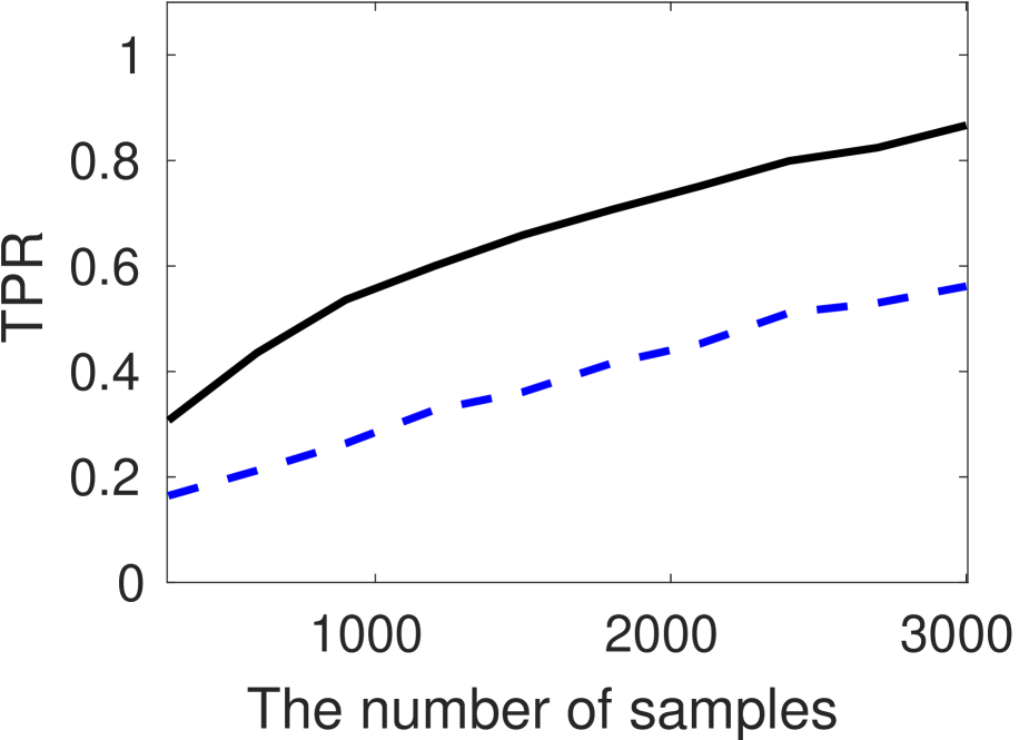
(c) Non-additive Non-linear.

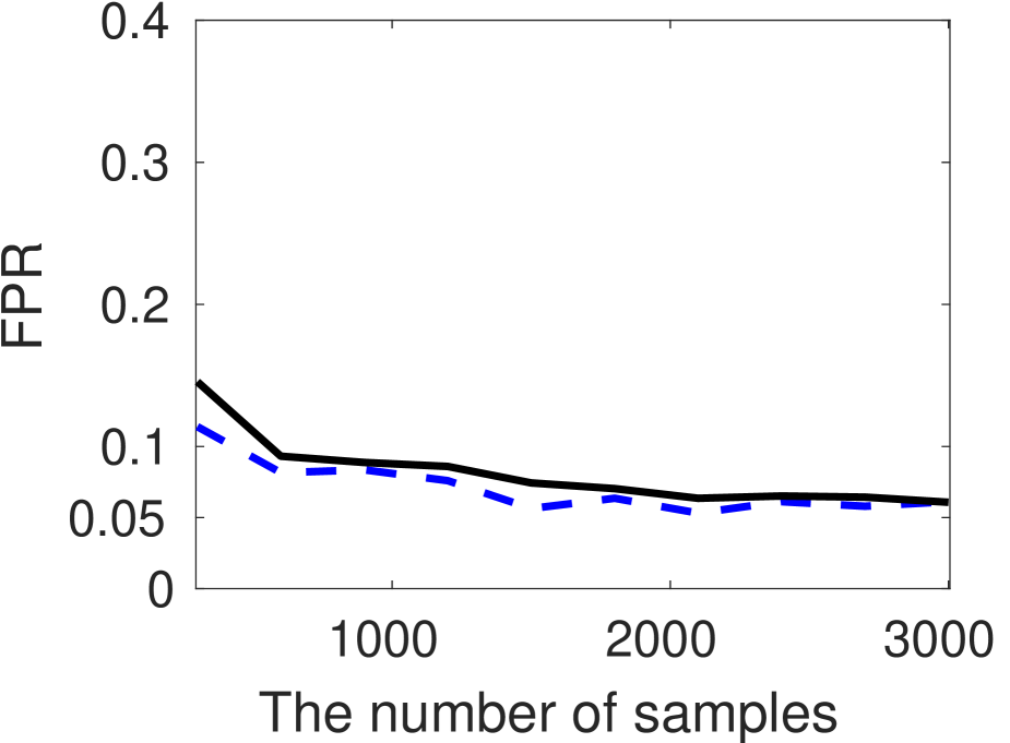
(d) Linear.

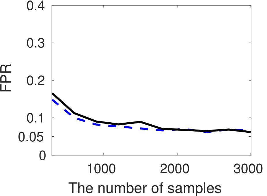
(e) Additive Non-linear.

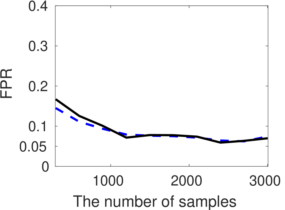
(f) Non-additive Non-linear.

Figure 3: The results for hsicInf in uni-variate setups with different block parameter $B$. (a)-(c): TPR for the three datasets. (d)-(f): FPR for the three datasets.

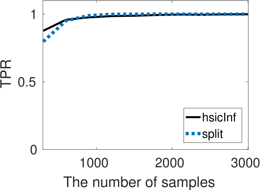
(a) Multi-variate (TPR).

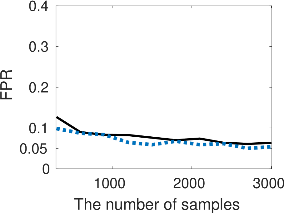
(b) Multi-variate (FPR).

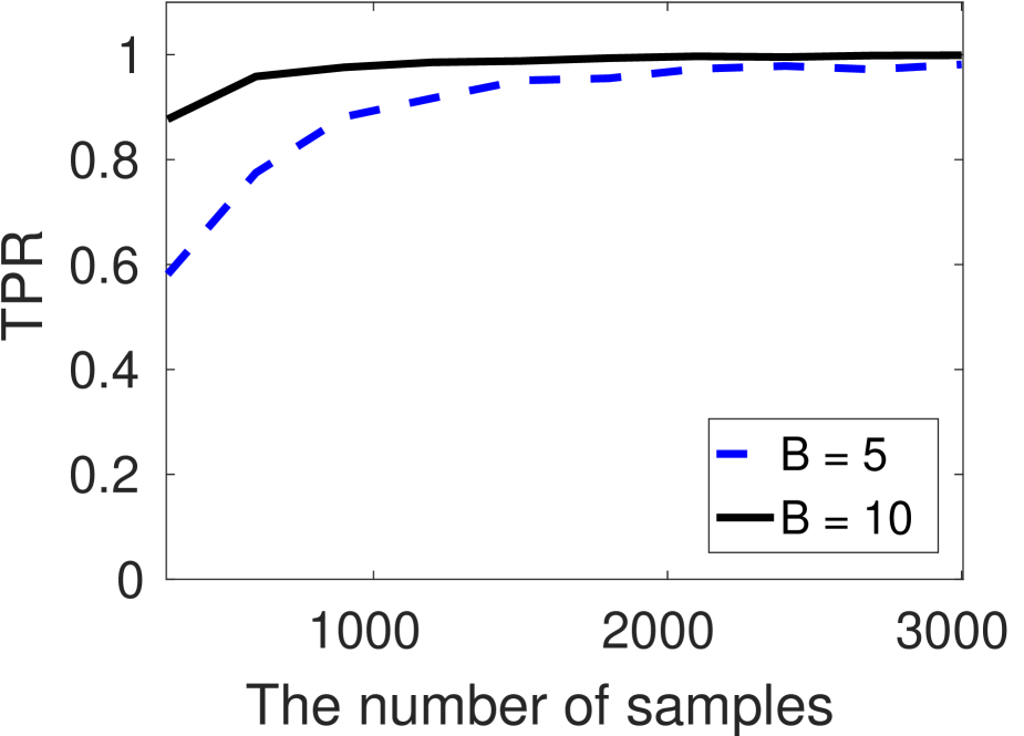
(c) hsicInf (TPR).

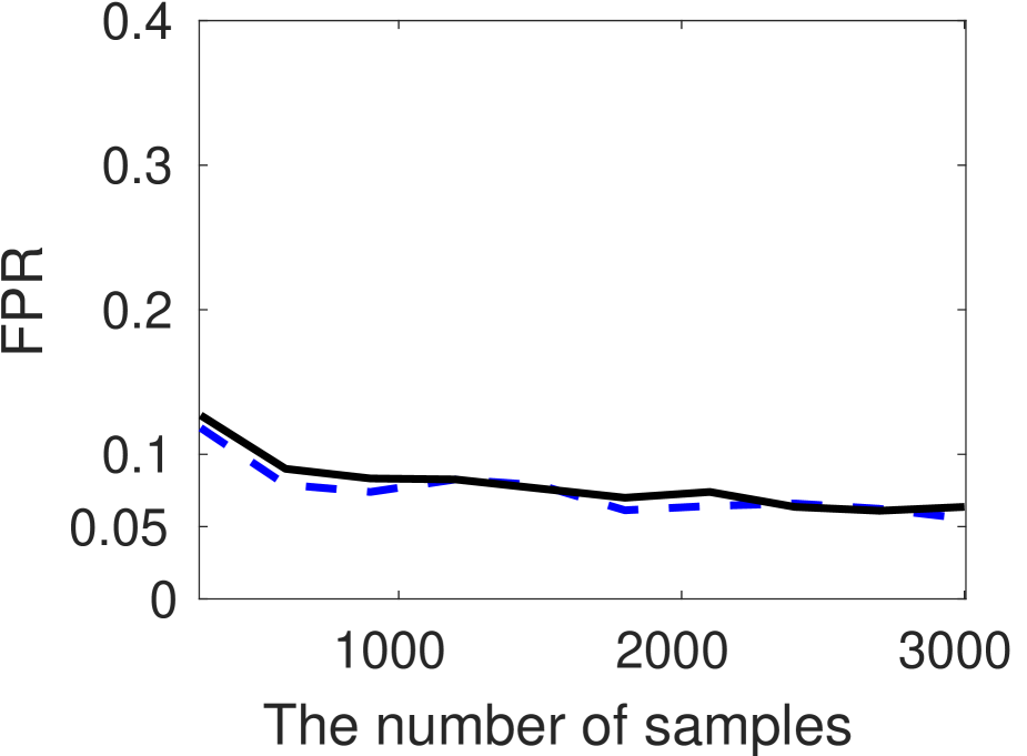
(d) hsicInf (FPR).

Figure 4: The results for the multi-variate regression dataset. (a)(b): TPRs and FPRs of hsicInf ($B=10$). (c)(d): TPRs and FPRs of hsicInf with different block size $B$.

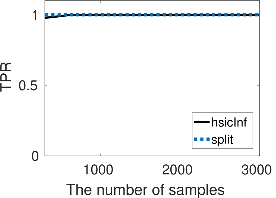
(a) Multi-class (TPR).

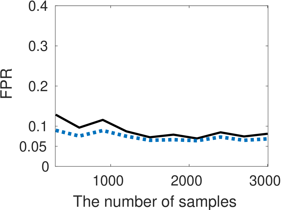
(b) Multi-class (FPR).

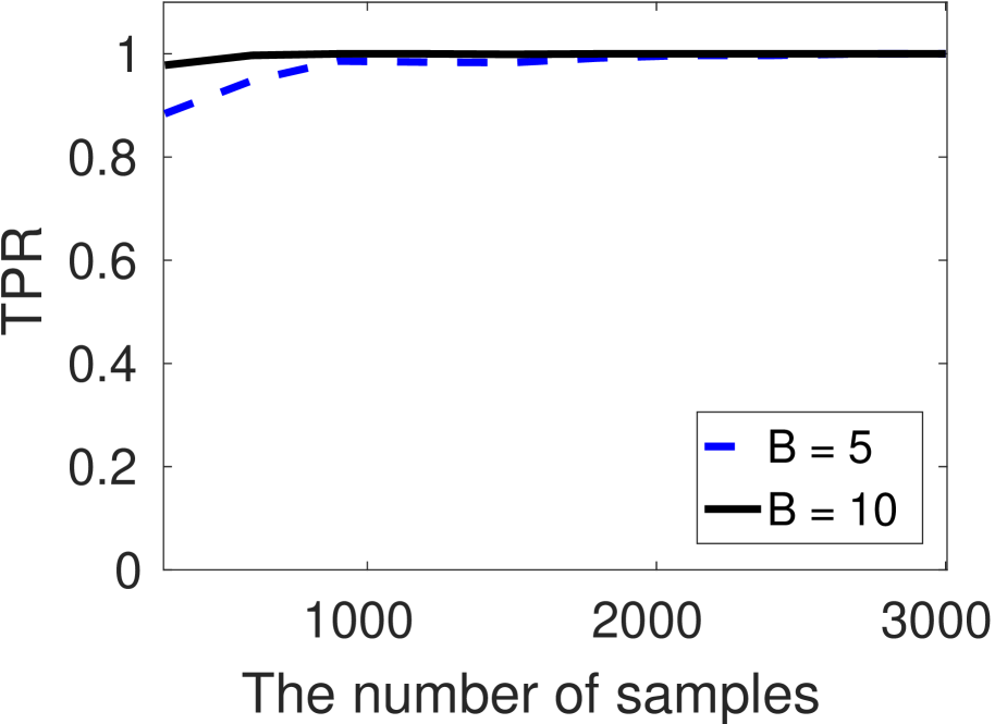
(c) hsicInf (TPR).

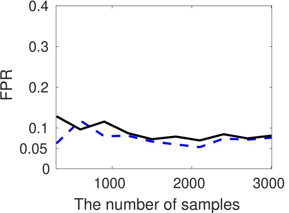
(d) hsicInf (FPR).

Figure 5: The results for the multi-class classification dataset.(a)(b): TPRs and FPRs of hsicInf ($B=10$). (c)(d): TPRs and FPRs of hsicInf with different block size $B$.

4.3 True positive rate comparison

Next, we compared the TPRs of hsicInf, split, and larInf.

4.3.1 Synthetic Data (Regression)

First, we evaluated whether the proposed method can find a set of statistically significant features from uni-variate linear/non-linear regression problems.

For this experiment, we first generated the input matrix ${\bm{X}}=[{\bm{x}}_{1},\ldots,{\bm{x}}_{n}]\in\mathbb{R}^{20\times n}$ where ${\bm{x}}\sim N({\bm{0}},\bar{{\bm{\Sigma}}})$, $[\bar{{\bm{\Sigma}}}]_{ij}=0.95\delta_{ij}+0.05,i,j\in\{1,2,3,4,5\},[\bar{{\bm{\Sigma}}}]_{ii}=\delta_{ij},i,j\in\{6,\ldots,20\}$, $\delta_{ij}=1$ if $i=j$ and 0 otherwise, and $n=\{300,600,\ldots,3000\}$.

Then, we generated the corresponding output variable as

• Linear: $Y=\sum_{i=1}^{5}X_{i}+0.1E$,

• Additive Non-linear: $Y=\sum_{i=1}^{5}X_{i}^{2}+0.1E$,

• Non-additive Non-linear: $Y=X_{1}\exp(X_{2})X_{3}\exp(X_{4})X_{5}+0.1E$,

where $E\sim N(0,1)$ is a random variable.

Figure 2 (a)-(c) show TPRs of all methods. As we expected, the proposed hsicInf has higher TPRs compared to the data-splitting method split, since the proposed method can use larger number of samples than split for selecting features. Figure 2 (d)-(f) show FPRs of all methods. Here, all the HSIC based approaches have larger FPRs than the significance level when the number of samples are small. This is due to the violation of the Gaussian assumption. hsicInf with small number of samples is an important future work.

The linear method larInf can select features for only linear setups, and it fails for non-linear counterparts. In contrast, the proposed algorithm can successfully detect statistically significant features for all setups.

Figures 3 shows that TPRs and FPRs of hsicInf with different block size $B$, respectively. These results indicate that the larger $B$ is usually preferable for having high detection power.

Table 1: The $p$-values computed by hsicInf from the Turkiye Student Evaluation dataset.

Feature description	$p$-value
The Instructor treated all students in a right and objective manner.	$>0.001$
The Instructor arrived on time for classes.	0.033
The Instructor’s knowledge was relevant and up to date.	0.018
The Instructor was open and respectful of the views of students about the course.	0.042
The Instructor demonstrated a positive approach to students.	0.033
The Instructor has a smooth and easy to follow delivery/speech.	0.186
The Instructor encouraged participation in the course.	0.037
The Instructor’s evaluation system effectively measured the course objectives.	0.176
The course aims and objectives were clearly stated at the beginning of the period.	0.452
The Instructor explained the course and was eager to be helpful to students.	0.463

4.3.2 Synthetic Data (Multi-variate regression)

We evaluated the proposed algorithm for multi-variate non-linear regression problems. Since existing PSI methods cannot be used for multi-variate regression problems, we only reported the HSIC based approaches.

We used the zero-mean multi-variate Gaussinan input matrix with $[\bar{{\bm{\Sigma}}}]_{ij}=0.95\delta_{ij}+0.05,i,j\in\{1,2,3,4\},[\bar{{\bm{\Sigma}}}]_{ii}=\delta_{ij},i,j\in\{5,\ldots,20\}$. For the output variable, we generated the three dimensional output variables as

$$Y_{1} =X_{1}+2X_{2}+0.1E,$$

$$Y_{2} =2X_{1}+X_{2}^{2}+0.1E,$$

$$Y_{3} =X_{3}\exp(2X_{4})+0.1E.$$

In this experiment, we have the training set $\{({\bm{x}}_{i},{\bm{y}}_{i})\}_{i=1}^{n}$ where ${\bm{x}}\in\mathbb{R}^{20}$ and ${\bm{y}}\in\mathbb{R}^{3}$.

Figure 4 shows TPRs and FPRs for the multi-variate regression case. As can be seen, both proposed methods can select statistically significant features.

4.3.3 Synthetic Data (Multi-class Classification)

We applied our proposed algorithm to a non-linear three-class classification problem. Again, there is no existing multi-class PSI algorithm, and thus, we here simply reported the performance of the HSIC based algorithms.

In this experiment, we generated a three-class classification dataset as

$$p({\bm{x}}^{(1,2)}|y=1) =N\left(\left[\begin{array}[]{c}-3\\ 0\\ \end{array}\right],\left[\begin{array}[]{cc}1&0\\ 0&1\\ \end{array}\right]\right)$$

$$p({\bm{x}}^{(1,2)}|y=2) =N\left(\left[\begin{array}[]{c}3\\ 0\\ \end{array}\right],\left[\begin{array}[]{cc}1&0\\ 0&1\\ \end{array}\right]\right)$$

$$p({\bm{x}}^{(1,2)}|y=3) =0.5N\left(\left[\begin{array}[]{c}0\\ 3\\ \end{array}\right],\left[\begin{array}[]{cc}1&0\\ 0&2.25\\ \end{array}\right]\right)$$

$$\phantom{=}+0.5N\left(\left[\begin{array}[]{c}0\\ -3\\ \end{array}\right],\left[\begin{array}[]{cc}1&0\\ 0&2.25\\ \end{array}\right]\right).$$

Then, we generated the final feature ${\bm{x}}=[({\bm{x}}^{(1,2)})^{\top}~{}\widetilde{{\bm{x}}}^{\top}]^{\top}$ where $\widetilde{{\bm{x}}}\in\mathbb{R}^{18}$ and $\widetilde{{\bm{x}}}\sim N({\bm{0}},{\bm{I}})$.

Figure 5 shows the TPR and FPR for the three-class classification problem, and the hsicInf algorithm can perfectly detect the important features.

4.4 Real-world data

Finally, we evaluated our proposed method on the Turkiye Student Evaluation Data Set (Gunduz and Fokoue, 2013).

This dataset consists of 5820 samples with 28 features. We used the ”Level of difficulty of the course as perceived by the student ($\{1,2,\ldots,5\}$)” as the output variable, and selected features that are significantly affected to the difficulty of the course. In this experiment, we set the number of selected features $k=10$, the block size $B=10$, and used the Gaussian kernel for output. Note that, since the output variable takes integers and are non-Gaussian, larInf cannot be used for this data.

Table 1 shows the selected features by hsicInf. As can be seen, the difficulties of class are highly related to the attitude of teachers and teacher’s support to students, and this result is reasonable.

5 Conclusion

In this paper, we proposed a novel post selection inference (PSI) algorithm hsicInf. The key advantage of the proposed method is that it can select a statistically significant features from non-linear and/or multi-variate data and have high detection power. To the best of our knowledge, this is the first work to address the PSI algorithm for both nonlinear and multi-variate regression problems. Through several experiments, we showed that the proposed method outperformed a state-of-the-art linear PSI algorithm.

References

- Balasubramanian et al. (2013) K. Balasubramanian, B. Sriperumbudur, and G. Lebanon. Ultrahigh dimensional feature screening via RKHS embeddings. In AISTATS, 2013.
- Berk et al. (2013) R. Berk, L. Brown, A. Buja, K. Zhang, and L. Zhao. Valid post-selection inference. The Annals of Statistics, 41(2):802–837, 2013.
- Cover and Thomas (2006) T. M. Cover and J. A. Thomas. Elements of Information Theory. John Wiley & Sons, Inc., Hoboken, NJ, USA, 2nd edition, 2006.
- Efron et al. (2004) B. Efron, T. Hastie, I. Johnstone, and R. Tibshirani. Least angle regression. The Annals of statistics, 32(2):407–499, 2004.
- Fan and Lv (2008) J. Fan and J. Lv. Sure independence screening for ultrahigh dimensional feature space. Journal of the Royal Statistical Society: Series B (Statistical Methodology), 70(5):849–911, 2008.
- Fan et al. (2013) J. Fan, Y. Liao, and M. Mincheva. Large covariance estimation by thresholding principal orthogonal complements. Journal of the Royal Statistical Society: Series B (Statistical Methodology), 75(4):603–680, 2013.
- Forman (2008) G. Forman. BNS feature scaling: An improved representation over TF-IDF for SVM text classification. In CIKM, 2008.
- Fukumizu et al. (2004) K. Fukumizu, F. R. Bach, and M. I. Jordan. Dimensionality reduction for supervised learning with reproducing kernel hilbert spaces. Journal of Machine Learning Research, 5(Jan):73–99, 2004.
- Fukumizu et al. (2008) K. Fukumizu, A. Gretton, X. Sun, and B. Schölkopf. Kernel measures of conditional dependence. In NIPS, 2008.
- Gretton et al. (2005) A. Gretton, O. Bousquet, Alex. Smola, and B. Schölkopf. Measuring statistical dependence with Hilbert-Schmidt norms. In ALT, 2005.
- Gunduz and Fokoue (2013) N. Gunduz and E. Fokoue. UCI machine learning repository, 2013.
- Hastie et al. (2015) T. Hastie, R. Tibshirani, and M. Wainwright. Statistical learning with sparsity: the lasso and generalizations. CRC Press, 2015.
- Lee and Taylor (2014) J. D. Lee and J. E. Taylor. Exact post model selection inference for marginal screening. In NIPS, 2014.
- Lee et al. (2016) J. D. Lee, D. L. Sun, Y. Sun, and J. E. Taylor. Exact post-selection inference, with application to the lasso. The Annals of Statistics, 44(3):907–927, 2016.
- Lockhart et al. (2014) R. Lockhart, J. Taylor, R. J. Tibshirani, and R. Tibshirani. A significance test for the lasso. Annals of statistics, 42(2):413, 2014.
- Ravikumar et al. (2009) P. Ravikumar, J. Lafferty, H. Liu, and L. Wasserman. Sparse additive models. Journal of the Royal Statistical Society: Series B (Statistical Methodology), 71(5):1009–1030, 2009.
- Shenoy et al. (2008) P. Shenoy, K. J. Miller, B. Crawford, and R. N. Rao. Online electromyographic control of a robotic prosthesis. IEEE Transactions on Biomedical Engineering, 55(3):1128–1135, 2008.
- Song et al. (2012) L. Song, A. Smola, A. Gretton, J. Bedo, and K. Borgwardt. Feature selection via dependence maximization. JMLR, 13:1393–1434, 2012.
- Sriperumbudur et al. (2011) B. K. Sriperumbudur, K. Fukumizu, and G. RG. Lanckriet. Universality, characteristic kernels and RKHS embedding of measures. Journal of Machine Learning Research, 12(Jul):2389–2410, 2011.
- Taylor and Tibshirani (2016) J. Taylor and R. Tibshirani. Post-selection inference for l1-penalized likelihood models. arXiv preprint arXiv:1602.07358, 2016.
- Taylor and Tibshirani (2015) Jonathan Taylor and Robert J Tibshirani. Statistical learning and selective inference. Proceedings of the National Academy of Sciences, 112(25):7629–7634, 2015.
- Tibshirani (1996) R. Tibshirani. Regression shrinkage and selection via the Lasso. Journal of the Royal Statistical Society, Series B, 58(1):267–288, 1996.
- Xing et al. (2001) E. P. Xing, M. I. Jordan, R. M. Karp, et al. Feature selection for high-dimensional genomic microarray data. In ICML, 2001.
- Yamada et al. (2014) M. Yamada, W. Jitkrittum, L. Sigal, E. P. Xing, and M. Sugiyama. High-dimensional feature selection by feature-wise kernelized lasso. Neural computation, 26(1):185–207, 2014.
- Zhang et al. (2016) Q. Zhang, S. Filippi, A. Gretton, and D. Sejdinovic. Large-scale kernel methods for independence testing. arXiv preprint arXiv:1606.07892, 2016.