Decision trees unearth return sign correlation in the S&P 500

Abstract

Technical trading rules and linear regressive models are often used by practitioners to find trends in financial data. However, these models are unsuited to find non-linearly separable patterns. We propose a decision tree forecasting model that has the flexibility to capture arbitrary patterns. To illustrate, we construct a binary Markov process with a deterministic component that cannot be predicted with an autoregressive process. A simulation study confirms the robustness of the trees and limitation of the autoregressive model. Finally, adjusting for multiple testing, we show that some tree based strategies achieve trading performance significant at the 99% confidence level on the S&P 500 over the past 20 years. The best strategy breaks even with the buy-and-hold strategy at 21 bps in transaction costs per round trip. A four-factor regression analysis shows significant intercept and correlation with the market. The return anomalies are strongest during the bursts of the dotcom bubble, financial crisis, and European debt crisis. The correlation of the return signs during these periods confirms the theoretical model.

C01, C12, C14, C15, C22, G01, G14, G17

1 Introduction

The efficient market hypothesis (Fama, 1970, 1991) is a cornerstone of theoretical finance that has been widely debated and tested. The hypothesis states that market prices instantaneously and fully reflect all available information. Mathematically speaking, market returns follow a martingale process after adjusting for equilibrium expected returns. As a consequence, in an efficient market it is impossible to develop trading strategies that are consistently profitable in excess of the buy-and-hold strategy. However, real markets do not meet some necessary conditions for the Efficient Market Hypothesis (EMH) such as no transaction costs, and cost-less availability of information to all market participants. In contrast, real markets are better described as being in an equilibrium state of disequilibrium (Grossman and Stiglitz, 1980), in which a perpetual flow of new events needs to be constantly arbitraged to keep markets marginally efficient. In particular, the recurring occurrence of bubbles and crashes (i.e. dotcom bubble, financial crisis, Chinese stock market turbulence) supports the hypothesis that irrational investors can provoke large departures from rational and efficient markets (Johansen et al., 2000; Malkiel, 2003; Sornette, 2003; Harras and Sornette, 2011).

The EMH cannot be proven true in general, but can be proven false by finding a sensible trading strategy significantly profitable in excess of the benchmark. To reject the null hypothesis of efficient markets, White (2000) proposed the reality check method that computes the statistical significance of the best trading strategy in a universe of strategies. The reality check method determines if the best strategy outperforms a given benchmark strategy, while accounting for the exact dependency structure of all tested strategies. This method has since been extended by Romano and Wolf (2005) to reject as many null hypotheses as possible while controlling for the familywise error rate. As well, they advocate the use of studentized test statistics to improve robustness in finite samples. Refinements for Heteroskedasticity and Auto-Correlation (HAC) robust performance metrics have been established by Ledoit and Wolf (2008).

The existing studies assessing the EMH using a multiple-testing framework provide a heterogeneous picture. The study by White (2000) finds no significant technical trading rule during a three year time span on the S&P 500. This result is confirmed by Sullivan et al. (1999) on a 10 year time period on the S&P 500, however they find significant trading rules on the Dow Jones for a 100 year time period ending in 1996. Subsequently, Hsu and Kuan (2005) analyze an extended universe of strategies and find no significantly performing strategy on the Dow Jones and S&P 500 during the period 1990-2000. However, they find significant trading rules for the more recent NASDAQ and Russell 2000 during the same period. Later, Hsu et al. (2010) compare the pre-ETF and post-ETF period for the U.S. and emerging markets. The post-ETF period is found to be fairly efficient, and in both periods emerging markets are found to be less efficient then the more mature U.S. markets. The efficiency check of foreign exchange markets by Hsu et al. (2016) reveals that technical trading has been profitable in the past, but returns have been declining. As for stock markets, the foreign exchanges of emerging countries are less efficient then in developed countries.

The picture is equally mixed when analyzing funds. The analysis by Fama and French (2009) shows that during the period of 1984 to 2006 mutual funds underperform in aggregate the three-factor, and four-factor benchmarks by about the transaction costs. When looking at the individual performance, even the best performers are not statistically significant. The study of Barras et al. (2005) mitigates this picture, finding significantly performing funds prior to 1996, and almost none afterwards. This result supports the stock market studies discussed above that showed increasing efficiency over time. In contrast, the portfolio approach by Yen et al. (2015) to measure fund performance does find significant performance during a 10 year period ending in 2007.

We note that the finding of statistically significant strategies does not necessarily reject the EMH. A statistically significant strategy is a necessary condition to reject the EMH, but it is not sufficient as traders may have been unable to select the best strategy ex-ante. To cover this aspect, the EMH definition of Timmermann and Granger (2004) requires a set of search technologies among which one would have selected the strategy to use. In practical terms, there must exist a sensible search technology that would have selected a profitable strategy. A search technology can as well be a portfolio of strategies that is rebalanced periodically, and generates statistically significant profits.

The existing assessments of the EMH are focused on testing the performance of technical trading strategies and funds. However, the anomalies reported by Niederhoffer and Osborne (1966), Zhang (1999), Leung et al. (2000), Andersen and Sornette (2005), Zunino et al. (2009), Satinover and Sornette (2012a, b) and James et al. (2014) have not undergone a rigorous analysis to the best of our knowledge. These anomalies are particularly interesting because many linearly inseparable patterns, as for example the logical exclusive-OR function (XOR), would remain undetected with linear models such as moving averages. Nonetheless, such patterns can be detected using statistical learning models such as decision trees.

In this paper, we demonstrate the limitation of autoregressive models to capture the predictable XOR pattern, and show how decision tree based models overcome this limitation. We carefully discuss different variants of decision trees and how to avoid the issue of overfitting. Especially, we derive the connection between fixed decision trees and Markov chains. The connection is used to derive a binary Markov process of order $\varrho$, analogous to the autoregressive process of order $\varrho$, but with more intricate non-linear autocorrelation patterns. We then prove that the parameters of an autoregressive process of order $\varrho$ have zero expectation for a binary Markov process satisfying certain conditions.

To confirm the theoretical results, we simulate the statistical significance of the competing models on an autoregressive process of order two and a binary Markov process of order two. The statistical significance is studied based on the studentized Sharpe ratio as a function of the sample size, the calibration window length, and the autocorrelation parameters. The simulation results show that the autoregressive forecast is optimal on the autoregressive process, but has no forecasting power on the binary Markov process. The fixed regression and classification trees are more robust, performing equally well on both processes. The regression and classification trees with dynamically optimized decision boundaries are prone to overfitting and underperform the fixed trees.

Finally, all competing model are tested on daily returns of the S&P 500 from Jan. 1, 1995 to Dec. 31, 2015. The multiple testing adjusted and HAC robust statistical significance of a trading strategy, derived from a forecasting model, is computed by combining the methodologies described in Romano and Wolf (2005) and Ledoit and Wolf (2008). Each model is tested for a range of lags and calibration window length, leading to a universe of 1000 strategies. The null hypothesis of no predictability for the best strategy is rejected at the 99% confidence level. The best performing model breaks even with the buy-and-hold strategy at transaction costs per round trip of 21.4 bps. This profitability threshold exceeds the 5 bps in transaction costs applied nowadays on the future market.

This paper continues as follows, Section 2 presents the competing autoregressive and tree based models. Section 3 provides analytical comparisons for the forecasting power of the autoregressive and tree based models. Section 4 presents the HAC robust multiple testing methodology used to computed p-values adjusted for data snooping. Sections 5 and 6 show the simulation results, respectively the empirical results. The last section concludes and outlines a path for future research.

2 Motivating Tree Based Forecasting

2.1 Linear Filter Models & Technical Trading Rules

Wold’s decomposition theorem (Mills and Markellos, 2008; Hamilton, 1994) states that every weakly stationary, purely non-deterministic stochastic process $\left\{X_{t}\right\}$ can be written as a linear filter with infinite lag. All time series analysis models defined as a finite-order stochastic difference equation derive from this general concept. The simplest stationary models being the autoregressive model $\textrm{AR}(\varrho)$ and moving average model $\textrm{MA}(\varrho)$ of order $\varrho$. Non-stationary models can be built using nested stationary models for the mean and variance.

These models of stochastic processes are foremost characterized by the autocorrelation function of returns and absolute returns. While these characteristics are predominantly used to described financial returns, several stylized facts such as gain/loss asymmetry and heavy tails are well document (Cont, 2001). The gain/loss asymmetry is often described by the skewness of the return distribution and the heavy tails by the kurtosis. However, possible non-linear dependencies are often neglected.

Non-linear stochastic processes arise when their representation is obtained by some non-linear mechanism, for example polynomial dependencies in the innovation, asymmetric innovations, correlated innovations, time varying parameters, or regime switching. Unfortunately, testing for non-linearity is a challenging task and not possible in general when the functional form of the non-linearity is unknown (Mills and Markellos, 2008, chap. 6). Past efforts have been concentrated on modeling the common stylized facts such as skewness, fat tails, volatility clustering, and regime switching, using non-linear combinations of linear filter models (Mills and Markellos, 2009). This continued use of linear models as building blocks for non-linear models leaves the possibility that deterministic non-linearly separable patterns have remained undetected in past studies

To forecast trends in stock markets, traders have developed an extensive taxonomy of technical trading rules expressing their beliefs about the market behavior. Some of these rules rely on a linear filter model such as moving average, which forecasts a trend persistency. While a majority of rules define trading triggers based on support and resistance bands, channels, and oscillators, these rules do not focus on a potential intrinsic structure of market returns, but on prices levels psychologically important to a large number of traders. Assuming that a majority of market participants acts based on these price levels, these rules should have significant profitability.

A common feature of linear filter models and technical trading rules is that they do not test for some potential non-linear dependencies. An example are the return sign correlation, which have been well documented by Christoffersen and Diebold (2003) and Christoffersen et al. (2006). In this section, we argue that return sign correlations can remain undetected in the autocorrelation function, and propose decision trees as a forecasting model to detect return sign correlations.

2.2 From Autoregressive to Tree Based Models

The autoregressive model $\textrm{AR}(\varrho)$ defines the evolution of the time series $\left\{X_{t}\right\}$ with $\varrho$ lags as

$$X_{t}=\phi_{0}+\sum_{i=1}^{\varrho}\phi_{i}X_{t-i}+a_{t},$$ (1)

with parameters $\phi=\left(\phi_{0},\,\phi_{1},\,\ldots,\,\phi_{\varrho}\right)$, and i.i.d. innovations $a_{t}$. The shortcoming of autoregressive models can be illustrated with the two argument exclusive-OR function $XOR(r_{-1},\,r_{-2})$ that returns true ($=1$) when exactly one of the arguments is true and false ($=-1$) otherwise (see Figure 1). An example of XOR like data is

$$\mathbf{X}=\left\{\left(\left(1,\,1\right),\,-1\right),\,\left(\left(1,\,-1\right),\,1\right),\,\left(\left(-1,\,1\right),\,1\right),\,\left(\left(-1,\,-1\right),\,-1\right)\right\},$$ (2)

where the four samples are assumed to be at independent times. The notation of Equation (2) is taken from the statistical learning literature (James et al., 2014), where $\mathbf{X}$ is the training data available, and $\left(\left(X_{t-2},\,X_{t-1}\right),\,X_{t}\right)$ denotes the sample at time $t$ with input $x_{t}=\left(X_{t-2},\,X_{t-1}\right)$ and output (=response) $y_{t}=X_{t}$. Calibrating the autoregressive model of order two to the data of Equation (2) yields the parameters

$$\left(\phi_{0}=0,\,\phi_{1}=0,\,\phi_{2}=0\right),$$ (3)

which fail at capturing the deterministic XOR function. As we will discuss in section 3.2, almost XOR like patterns can arise in time series data.

Non-linearly separable patterns can be modeled using a partition $R=\left\{R_{1},\,\ldots,\,R_{n}\right\}$ of the input (or feature) space into $n$ regions, and assigning the constant values $\left\{c_{1},\,\ldots,\,c_{n}\right\}$ to each region. The resulting evolution of the time series $X_{t}$ can then be written as

$$y_{t}=X_{t}=\sum_{i=1}^{n}c_{i}\cdot I\left\{x_{t}\in R_{i}\right\}+a_{t},$$ (4)

where $I$ is the indicator function, and $a_{t}$ are i.i.d. innovations. This modeling approach allows for an arbitrary flexibility, as any function can be approximated to any precision with a sufficient number of regions. For example, the XOR data from Equation (2) can be modeled exactly by the two regions $R_{1}=\left\{x\in\mathbb{R}^{2}|x_{1}x_{2}\geq 0\right\}$ with $c_{1}=-1$, and $R_{2}=\left\{x\in\mathbb{R}^{2}|x_{1}x_{2}<0\right\}$ with $c_{2}=1$. The downside of this modeling approach is that the number of parameters increases arbitrarily with the number of regions, and a procedure to control for overfitting is required.

What remains unspecified in the stochastic process of Equation (4) is the algorithm to estimate the regions based on a given realization $\left\{X_{t}\right\}_{1}^{T}$ of a process. In general, regions of arbitrary shape and overlaps can be used. However, for the purpose of this study, decision tree models provide sufficient flexibility. Decision trees find rectangular regions, using a recursive splitting algorithm of the input space that minimizes a loss function for the given training data. While several variations of the splitting algorithms exist, we will focus on the most popular Classification And Regression Tree (CART) algorithm described by Hastie et al. (2001, chap. 9).

In the context of financial returns with low signal to noise ratio, finding the best tree is an NP-complete problem (Hyafil and Rivest, 1976) that is not computationally feasible. This stands in stark contrast to autoregressive models were the global optimum can be estimated. However, this is not an issue as the CART algorithm is nonetheless deterministic by using recursive binary splitting, and subsequent pruning. The algorithm always finds the same tree for a given training data, allowing practitioners to independently obtain the same forecast. The definition of the splitting algorithms for regression and classification are given below, as well as a discussion of robustness in the context of highly stochastic data.

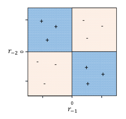
Figure 1: Illustration of the XOR pattern

2.3 Regression Tree Algorithm

The CART algorithm constructs a regression tree using the Mean Squared Error (MSE) as the loss function $Q_{MSE}\left(y,\,\hat{y}\right)=\left(y-\hat{y}\right)^{2}$. For a given training data $\mathbf{X}=\left\{\left(x_{1},\,y_{1}\right),\,\ldots,\,\left(x_{N},\,y_{N}\right)\right\}$ and partitioning of the input space into regions $R=\left\{R_{1},\,\ldots,\,R_{n}\right\}$, the algorithm assigns the response

$$\hat{c}_{i}=\left\langle\left\{y_{i}|x_{i}\in R_{i}\right\}\right\rangle$$ (5)

to region $R_{i}$, which is the mean observed output in that region. The binary splitting algorithm adds one new region at each iteration by splitting an existing region into two. At each iteration an existing region $R$ is split into two halves with a plane defined by variable $j$ and split point $s$ as

$$R^{1}\left(j,\,s\right)=\left\{x|x_{j}\leq s\right\}\>\textrm{and}\>R^{2}\left(j,\,s\right)=\left\{x|x_{j}>s\right\}.$$ (6)

The optimal split is given by

$$\min_{j,\,s}\left[\sum_{x_{i}\in R^{1}}Q\left(y_{i},\,\hat{c}_{1}\right)+\sum_{x_{i}\in R^{2}}Q\left(y_{i},\,\hat{c}_{2}\right)\right],$$ (7)

which can be determined efficiently by running through all the input variables and split points defined by the inputs.

In many scenarios, for example of XOR like training data, a split with not improvement in the loss can be followed by a split with a large reduction of the loss. This prevents the introduction of termination criterion in the splitting procedure. To overcome this issue, the fully grown tree $\mathcal{T}_{0}$ is subsequently pruned. The pruning procedure finds an optimal subtree $\mathcal{T}$ without the internal nodes that do not affect significantly the loss. The loss of a subtree $\mathcal{T}\subset\mathcal{T}_{0}$ is given by

$$Q\left(\mathcal{T},\,\alpha\right)=\sum_{m=1}^{\left|\mathcal{T}\right|}N_{m}Q_{m}\left(t\right)+\alpha\left|\mathcal{T}\right|,$$ (8)

where $Q_{m}\left(\mathcal{T}\right)=\frac{1}{N_{m}}\sum_{x_{i}\in R_{m}}Q\left(y_{i},\,\hat{c}_{m}\right)$ is the loss of the terminal node $m$, $N_{m}=\#\left\{x_{i}\in R_{m}\right\}$ is the number of samples in that node, and $\left|\mathcal{T}\right|$ is the number of terminal nodes in the tree. The regularization coefficient $\alpha$ of the tree size determines to which degree smaller trees are favored with respect to higher loss. The value $\alpha=0$ would yield the fully grown tree $\mathcal{T}_{0}$.

In the context of predicting financial returns, the signal to noise ratio in the samples is intrinsically low, and without appropriate pruning the data would be overfit. However, the Scikit-learn library (Pedregosa et al., 2011) used in this paper does not use a pruning parameter to control for overfitting, but instead allows us to set a lower bound on the number of samples in a terminal node. Fortunately, determining the adequate number of samples in a terminal node is simpler then determining an equivalent pruning parameter. The lower bound on the number of samples in a terminal node of a classification tree is computed in the following Section 2.4. The lower bound for a regression tree is set to the lower bound value of the equivalent classification tree.

We remark that the objective of the MSE loss function, namely minimizing variance within each region, is not necessarily optimal for forecasting financial returns. The suboptimality arises when the returns within a region exhibit low variance and mean close to zero. The insignificant mean implies that no forecast can be made. However, this does not negatively impact performance as return forecasts of small amplitude can be discarded as insignificant.

2.4 Classification Tree

The dominantly stochastic behavior of financial returns translates into particularly low statistical significance of regression model forecasts. However, the statistical significance of a potential signal can eventually be improved by mapping the outputs to categorical outputs. Under the assumption that the mapping removes more noise then signal, the resulting classification problem is more robust. The simplest such mapping is $r\rightarrow\textrm{sign}\left(r\right)$ that results in predicting only an up and down moves. The CART algorithm described in Section 2.3 only needs one modification for classification, namely a different loss function because the MSE loss is not suitable for classification. Typically, the classification of $K$ classes (e.g. $\left\{-,\,+\right\}$ with $K=2$) is performed using the Gini index $Q_{Gini}\left(\vec{p}\right)=\sum_{i\neq j}^{K}p_{i}p_{j}$, which maximizes the probability $p_{i}$ of a single class in a region.

In the context of predicting market up or down moves, the Gini index naturally sets the right objective, as it will maximize the predictability of an up or down move in a given region. However, the Gini index by itself is prone to overfitting, as terminal nodes with a few samples of the same kind are favored despite such nodes being a likely occurrence under the null hypothesis of no predictability. To alleviate this problem, we set a lower bound on the number of samples in a terminal node.

The probability distribution of $k$ up moves ($\uparrow$) and $n-k$ down moves ($\downarrow$), assuming equal class probability, is given by the binomial distribution

$$P\left(\#\uparrow=k,\,\#\downarrow=n-k\right)=\left(\frac{1}{2}\right)^{n}\left(\begin{array}[]{c}n\\ k\end{array}\right).$$ (9)

For sufficiently large $n$, this binomial distribution can be approximated by the normal distribution $\mathcal{N}\left(\frac{n}{2},\,\frac{1}{4n}\right)$. Now we compute $n$ assuming that the prediction is significant at the one standard deviation and the class probabilities satisfy $\left|p_{+}-p_{-}\right|=2\cdot 0.05$. This implies $\frac{1}{4n}=0.05^{2}$, or $n\geq 100$, which would require at least 100 samples per terminal node. This illustrates the difficulty of obtaining statistically significant forecasts and the large amount of calibration data required. In general, the minimum number of samples per terminal node should be picked as large as possible.

2.5 Fixed Tree

Similarly to the classification presented in Section 2.4, the signal to noise ratio in the input variables can be improved by a mapping of the inputs onto the two categories $\left\{-,\,+\right\}$. In case of inputs with $\varrho$ lags, this results in the discrete input space $\left\{-,\,+\right\}^{\varrho}$ with $2^{\varrho}$ elements. For a training set $\mathcal{D}$, the limited number of possible inputs controls the expected number of samples in a leaf $R$ as $E\left[N_{R}\right]=\frac{\left|\mathcal{D}\right|}{2^{p}}$. Therefore, with an appropriate choice of $\varrho$ with respect to the sample size $\left|\mathcal{D}\right|$, the problem of overfitting does not arise. This allows us to remove the lower bound on the number of samples per leaf, resulting in the CART algorithm to generate the fully grown tree with regions $\left\{R_{1},\,\ldots,\,R_{2^{\varrho}}\right\}$ (i.e. one region for each input). In other terms, the tree is fixed by the number of lags $\varrho$, and the CART algorithm reduces to compute the class probabilities in each leaf. A fixed tree can be used for classification, prediction of the majority vote inside each leaf, or regression by predicting the mean return of a leaf.

2.6 Probit Models & Polynomial Features

Probit models could be used as the autoregressive equivalent of classification trees, calibrating the parameters using only binary up and down returns. Nonetheless, just as the autoregressive model, the probit model cannot capture linearly inseparable patterns like the XOR function. To capture non-linear patterns, the autoregressive or probit models have to be extended with non-linear features. For example, the XOR function can be described with the quadratic feature $r_{t-1}\cdot r_{t-2}$.

However, polynomial features are not robust with respect to skewed distributions or multiple patterns offset with respect to the origin (e.g. offset as $\left(r_{t-1}-x_{1}\right)\left(r_{t-2}-x_{2}\right)$). In contrast, decision trees are non-linear predictors robust with respect to both issues. The CART algorithm can find localized non-linear predictability independently of its location in the input space, and use multiple regions to approximate skewness.

3 Comparing Forecasting Power

3.1 Connecting Fixed Trees to Markov Chains

Given a fixed decision tree, the time evolution defined by Equation (4) defines as well the transition probability $p$ from the sample at time $t$ to the sample at time $t+1$ as

$$\left(\left(X_{t-\varrho},\,\ldots,\,X_{t-1}\right),\,X_{t}\right)\overset{p}{\rightarrow}\left(\left(X_{t-\varrho+1},\,\ldots,\,X_{t}\right),\,X_{t+1}\right).$$ (10)

The sample inputs $\left(X_{t-\varrho},\,\ldots,\,X_{t-1}\right)$ define $2^{\varrho}$ possible states $\left\{S_{1},\,\ldots,\,S_{2^{\varrho}}\right\}$, and the time evolution defines the two possible transitions from each state to another state, while the remaining $2^{\varrho}-2$ states are unattainable. In other terms, the fixed decision tree defines a $\varrho$-th order Markov chain with $2^{\varrho}$ states, and two time dependent non-zero outgoing transition probabilities from each state.

We denote by $\boldsymbol{P}\in\left[0,\,1\right]^{2^{\varrho}\times 2^{\varrho}}$ the time independent transition matrix of the Markov chain defined by a fixed tree $\mathcal{T}$, resulting from the mapping of the returns onto the states $\left\{-,\,+\right\}$. The elements $\boldsymbol{P}_{ij}$ of the transition matrix describe the probabilities $P\left(S_{j}\rightarrow S_{i}\right)$ to go from state $S_{j}$ to state $S_{i}$. The probabilities to transition from one state to any of the states must always sum to one, imposing $\sum_{i=1}^{2^{\varrho}}\boldsymbol{P}_{ij}=1,\,\forall j$. Due to the particular structure of the tree, each state has two incoming transitions, and two outgoing transitions. This implies that each row and column in $\boldsymbol{P}$ has two non-zeros entries.

This Markov chain admits a stationary distribution if there exists a vector of probabilities $\pi\in\left[0,\,1\right]^{2^{\varrho}}$, satisfying $\left|\pi\right|=\sum_{i=1}^{2^{\varrho}}\left|\pi_{i}\right|=1$ and

$$\boldsymbol{P}\pi=\pi.$$ (11)

The component $\pi_{i}$ of the vector $\pi$ represents the probability to be in state $S_{i}$ at the stationary regime. The equality in Equation (11) asserts the stationarity condition that the probability of each state is invariant when transitioning to the next state. The stationary distribution $\pi$ is an eigenvector of $\boldsymbol{P}$ with unit eigenvalue. The eigenvalues $\left\{\lambda_{1},\,\ldots,\,\lambda_{2^{\varrho}}\right\}$ of $\boldsymbol{P}$ all satisfy $0\leq\lambda_{i}\leq 1$, and consequently the stationary distribution is always determined by the eigenstates (i.e. eigenvectors) with unit eigenvalues, while the eigenstates associated to eigenvalues $\lambda<1$ decay away. The second largest eigenvalue determines how quickly the stationary distribution is reached. Multiple eigenstates with unit eigenvalue arise in the case of reducible chains composed of several independent Markov chains. This can be shown by the orthogonality property of eigenstates and all their components being strictly positive in the context of Markov chains.

3.2 Binary Markov Based Processes

In the case of binary categories $\left\{-,\,+\right\}$, namely up ($X_{t}\geq 0$) and down ($X_{t}<0$) moves, the Markov chain defined in Section 3.1 has $2^{\varrho}$ possible states. Each state $S_{i}\in\left\{-,\,+\right\}^{\varrho}$ has two outgoing transitions probabilities $p_{i+}$ and $p_{i-}$, the probability of an up move, respectively a down move. These two outgoing probabilities are subject to $p_{i+}+p_{i-}=1$, and we can characterize them by a single variable $\Delta p_{i}=p_{i+}-p_{i-}$, where $p_{i+}=\frac{1}{2}\left(1+\Delta p_{i}\right)$ and $p_{i-}=\frac{1}{2}\left(1-\Delta p_{i}\right)$. Each state $S_{i}$ has as well two incoming transition probabilities, which we denote by $p_{+i}=P\left(S_{+i}\rightarrow S_{i}\right)$ and $p_{-i}=P\left(S_{-i}\rightarrow S_{i}\right)$, where the first index ($+$ or $-$) stands for the first sign of the previous state (e.g. $S_{i}=\left(-,\,+\right)$, $S_{+i}=\left(+,\,-\right)\rightarrow S_{i}$, and $S_{-i}=\left(-,\,-\right)\rightarrow S_{i}$). We remark that the sets of outgoing and incoming probabilities are in one-to-one correspondence. The duplicate definition of the transition probabilities is introduced for subsequent convenience.

The stationary distribution $\pi$ satisfies

$$\pi_{+i}\cdot p_{+i}+\pi_{-i}\cdot p_{-i}=\pi_{i},\,\forall 1\leq i\leq 2^{\varrho},$$ (12)

where $\pi_{+i}$ and $\pi_{-i}$ stand for the probabilities at stationarity of the state $S_{+i}$, respectively $S_{-i}$. We remark that the outgoing probabilities of each state must always sum to one, but the incoming probabilities can be arbitrary $p_{+i},\,p_{-i}\in\left[0,\,1\right]$. In the special case of incoming probabilities $p_{+i}+p_{-i}=1$, the stationary distribution is given by $\pi_{i}=\frac{1}{2^{\varrho}},\,\forall i$. In other terms, the stationary distribution with uniform probability for all states arises when the incoming probabilities of each state (i.e. rows in $\boldsymbol{P}$) sum to one. This result can be derived from Equation (11) by setting $\pi=\frac{1}{2^{\varrho}}\vec{1}$, which leads to $\boldsymbol{P}\frac{1}{2^{\varrho}}\vec{1}=\frac{1}{2^{\varrho}}\vec{1}\Rightarrow\sum_{j=1}^{2^{\varrho}}\boldsymbol{P}_{ij}=p_{+i}+p_{-i}=1,\,\forall i$.

Based on the Markov chain, we define the Data Generating Process (DGP)

$$X_{t+1}=\begin{cases}+\left|\mathcal{N}\left(a_{t+1}|\,0,\,\sigma\right)\right|&\textrm{with probability }p_{t+}\\ -\left|\mathcal{N}\left(a_{t+1}|\,0,\,\sigma\right)\right|&\textrm{with probability }p_{t-}\end{cases},$$ (13)

where $p_{t+}$ and $p_{t-}$ are the outgoing transition probabilities for the state $S_{t}$ at time $t$.

In order for this DGP to generate a continuous normal distribution, without jump at $X_{t}=0$, the number of up and down moves needs to be equal, which is enforced by the condition

$$B\left(\boldsymbol{P}\right)=\sum_{i=1}^{2^{\varrho}}\pi_{i}\Delta p_{i}=0.$$ (14)

As the stationary vector $\pi$ is a function of $\boldsymbol{P}$, the Equation (14) is a non trivial polynomial equation in $\boldsymbol{P}$. However, in the case where all states are equally likely, the balance of up and down moves is achieved when $\sum_{i=1}^{2^{\varrho}}\Delta p_{i}=0$.

We remark that the balancing condition is not the only possibility to obtain a continuous distribution. The balance between up and down moves can be broken locally as long as the balancing Equation (14) has expectation zero: $E\left[B\left(\boldsymbol{P}\right)\right]=0$. Assuming sufficiently low autocorrelation over time for the balancing term $B\left(\boldsymbol{P}\right)$, the discontinuity of the return distribution in finite samples cannot be detected in a statistically significant manner. Another possibility is to remove the discontinuity with an asymmetry of the left and right tail distribution. The later case is regularly observed in equity indices where up moves are more likely but the negative returns have a larger tail (i.e. distribution skewness).

Figure 2.a shows the binary Markov process with lag one ($\varrho=1$). Figure 2.b shows the two degrees of freedom in the binary Markov process with lag two ($\varrho=2$), uniform state probability, and equal number of up and down moves. When picking $\Delta p_{1}=0.5$ and $-0.5<\Delta p_{2}\ll 0$ the binary Markov process with two lags produces almost exactly the XOR pattern. The binary Markov processes with three and four lags have more then two degrees of freedom when fulfilling the uniform state probability and balancing conditions.

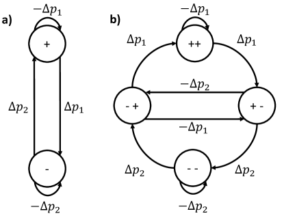
Figure 2: Illustration of binary Markov processes and associated parameters: a) one lag ($\varrho=1$); b) two lags ($\varrho=2$) and stationary regime with equal probabilities for all states.

3.3 Expected Autoregressive Forecast for Binary Markov Processes

The Markov DGP defined in Equation (13) violates the Martingale condition

$$E\left[X_{t+1}|X_{t-\varrho+1},\,\ldots,\,X_{t}\right]=0$$ (15)

when there exists a state $S_{i}$ such that $\Delta p_{i}\neq 0$. We want to determine to which degree the deterministic pattern can be predicted using an $\textrm{AR}(\varrho)$ autoregressive model as defined in Equation (1). Assuming homoskedasticity of the inputs $\boldsymbol{X}$ (not to be confused with the samples $\mathbf{X}$) and outputs $\boldsymbol{Y}$, the unbiased least square regression estimator reads

$$\hat{\phi}=\left(\boldsymbol{X}^{T}\boldsymbol{X}\right)^{-1}\boldsymbol{X}^{T}\boldsymbol{Y}.$$ (16)

To compute the expectation of this estimator for the binary Markov DGP we notice that for every state $S\in\boldsymbol{S}=\left\{-,\,+\right\}^{\varrho}$ there is a reverse state $-S$. Therefore, the set of states can be split into two as $\boldsymbol{S}=\boldsymbol{S}^{+}\boldsymbol{\cup}\boldsymbol{S}^{-}$, where $\left|\boldsymbol{S}^{+}\right|=\left|\boldsymbol{S}^{-}\right|$ and $S_{i}^{+}=-S_{i}^{-},\,\forall 1\leq i\leq 2^{\varrho-1}$. Each state is paired to its reverse. Assuming $n$ observed samples, the inputs $\boldsymbol{X}$ belong to the space $\boldsymbol{S}^{\times n}$, and the distribution of $\boldsymbol{Y}$ is defined by Equation (13). Using these assumptions we compute

$$E\left[\boldsymbol{X}^{T}\boldsymbol{Y}\right] = \sum_{i=1}^{2^{\varrho-1}}\alpha\left(\pi_{i}^{+}S_{i}^{+}p_{i+}^{+}+\pi_{i}^{-}S_{i}^{-}p_{i-}^{-}\right),$$ (17)

where $\alpha$ is a normalization factor stemming from the half-normal distribution of the variables. In the case of uniform probabilities for all states, the expectation simplifies to

$$E\left[\boldsymbol{X}^{T}\boldsymbol{Y}\right]=\frac{\alpha}{2^{\varrho}}\sum_{i=1}^{2^{\varrho-1}}S_{i}^{+}\left(p_{i+}^{+}-p_{i-}^{-}\right).$$ (18)

The condition $\Delta p_{i}^{+}=\Delta p_{i}^{-}$ implies $E\left[\boldsymbol{X}^{T}\boldsymbol{Y}\right]=0$ as $p_{i+}^{+}-p_{i-}^{-}=\frac{1}{2}\left(1+\Delta p_{i}^{+}-1-\Delta p_{i}^{-}\right)=0$, and at the same time fulfills the balancing condition of Equation (14). As a result, the estimated parameters $\hat{\phi}$ are zero, and the autoregressive model is unable to predict the deterministic pattern in the Markov process.

The binary Markov process with lag $\varrho=1$ only has the two states $\left\{-,\,+\right\}$, which can be split into $\boldsymbol{S}^{+}=\left\{+\right\}$ and $\boldsymbol{S}^{-}=\left\{-\right\}$, and is determined by the two parameters $\Delta p_{1}^{+}$ ($=\Delta p_{1}$) and $\Delta p_{1}^{-}$ ($=\Delta p_{2}$). This process has zero expectation for an autoregressive model when $\Delta p_{1}^{+}=\Delta p_{2}^{+}$, which implies the stationary regime $\pi_{+}=\pi_{-}=\frac{1}{2}$. However, the balancing condition of Equation (14) is incompatible as it is satisfied when $\Delta p_{1}^{+}=-\Delta p_{2}^{+}$. Nonetheless, as discussed in Section 3.2, the balancing condition is not necessary as the return distribution can be skewed.

The binary Markov process with two lags can satisfy the balancing condition and have zero expectation for an autoregressive process. The DGP including the degrees of freedom fulfilling these conditions are shown in Figure 2.b.

3.4 Expected Fixed Tree Forecast for Autoregressive Processes

Assuming an autoregressive DGP $\textrm{AR}(\varrho)$, we want to determine how well a fixed regression tree with $\varrho$ lags is able to predict the deterministic component arising when $\left\|\phi\right\|>0$. The fixed regression tree assigns to every of the $2^{\varrho}$ input states $S_{i}=\left(S_{i,\,1},\,\ldots,\,S_{i,\,\varrho}\right)\in\boldsymbol{S}$ the mean

$$\hat{c}_{i}=E\left[X_{t+1}|\textrm{sign}\left(X_{t-\varrho+1}\right)=S_{i,\,1},\,\ldots,\,\textrm{sign}\left(X_{t}\right)=S_{i,\,\varrho}\right].$$ (19)

In an autoregressive process with normally distributed innovations, the lagged variables are distributed as $x_{t}=\left(X_{t-\varrho+1},\,\ldots,\,X_{t}\right)\thicksim\mathcal{N}\left(0,\,\Lambda\left(\phi\right)\right)$, where $\Lambda\left(\phi\right)\in\mathbb{R}^{\varrho}$ is the covariance matrix of the $\varrho$ lags, assuming the independent innovations are distributed as $a_{t}\thicksim\mathcal{N}\left(0,\,\sigma\right)$.

Due to the autocorrelation, there is a directional bias of the return dependent of the previous $\varrho$ returns. This bias can be computed for a region $R_{i}=\left\{x\in\mathbb{R}^{\varrho}|x_{j}S_{i\,j}\geq 0,\,\forall j\right\}$ to be

$$P\left(y_{t}\geq 0|x_{t}\in R_{i}\right)=\int_{R_{i}}\mathcal{N}\left(x|\,0,\,\Lambda\left(\phi\right)\right)\int_{-\phi\cdot x}^{+\infty}\mathcal{N}\left(a|\,0,\,\sigma\right)dxda.$$ (20)

In the general case of an arbitrary autoregressive parameter $\phi$, this integral cannot be evaluated in closed form.

The simplest case $\textrm{AR}(1)$ has the analytically solution

$$P\left(y_{t}\geq 0|x_{t}\in R_{+}\right)=\frac{1}{2}+\frac{1}{\pi}\arctan\left(\frac{\phi}{1-\phi^{2}}\right),$$ (21)

where $R_{+}=\mathbb{R}^{+}$. As expected, the bias is independent of the variance of the innovations. The directional bias for the region $R_{-}=\mathbb{R}^{-}$ is obtained by symmetry as $P\left(y_{t}\geq 0|x_{t}\in R_{-}\right)=1-P\left(y_{t}\geq 0|x_{t}\in R_{+}\right)$. Assuming the calibration data is sufficient for a decision tree to predict the bias correctly every time, the directional accuracy of the tree will be $P\left(y_{t}\geq 0|x_{t}\in R_{+}\right)$. An $\textrm{AR}(1)$ predictor with correct parameter $\phi$ always makes the same prediction as a decision tree in this scenario, and therefore the two predictors have identical directional accuracy. As an example, for $\phi=0.1$ the directional accuracy is $\approx 0.532$.

Determining the directional accuracy for the $\textrm{AR}(2)$ case leads to integrals over multivariate distribution that cannot be solved in closed form. Hence, only numerical solutions are possible and would require a lengthy computation analyzing each region separately. Nonetheless, let us remark what happens in the regions $R_{+-}$ and $R_{-+}$ for the parameter choice $\phi=\left(\phi_{0}=0,\,\phi_{1},\,\phi_{2}=\phi_{1}\right)$. The value of $\phi\cdot x$ for $x=\left(x_{1},\,x_{2}\right)\in R_{+-}$ is anti-symmetric with respect to the axis $x_{2}=-x_{1}$. As a consequence of this anti-symmetry, the integral defined in Equation (20) takes the constant value $P\left(y_{t}\geq 0|x_{t}\in R_{i}\right)=\frac{1}{2}$, and this region has no predictability bias for a fixed tree. However, the regions $R_{++}$ and $R_{--}$ exhibit a predictability bias similar to the $\textrm{AR}(1)$ case, and therefore the fixed tree predictor will have roughly half the directional accuracy of the autoregressive predictor in this specific case. Hence, fixed trees can be a sub-optimal choice to predict autoregressive processes with two lags or more. Nonetheless, they are more robust then autoregressive models, which are entirely unable to predict a binary Markov process. Additionally, the CART algorithm can generate a regression tree approximating arbitrarily well the autoregressive process, assuming sufficient calibration data is available. In reverse, the autoregressive model is always too rigid to capture the binary Markov process.

4 Statistical Test

4.1 Multiple Testing Methodology

In this study, we aim to determine the significance level at which a strategy outperforms a given benchmark. In particular in the context of multiple testing with correlated strategies, as we want to test the predictive power of the decision tree and autoregressive models for different lags and calibration window lengths. This goal can be achieved using the stepwise multiple testing method developed by Romano and Wolf (2005). It acts on the observed data matrix $\left(X_{T,\,\mathcal{S}+1}\right)_{t,\,s}$ (i.e. returns), with $1\leq t\leq T$ time steps of the $1\leq s\leq\mathcal{S}$ different strategies. The last column $\mathcal{S}+1$ is reserved for the benchmark. The distribution of a chosen performance metric is computed using bootstrapped realizations of $X_{T,\,\mathcal{S}+1}$. Then a stepwise procedure rejects as many null hypothesis as possible, at a given significance level $\alpha$, without violating the familywise error rate.

4.2 Test Statistic

To determine the risk adjusted performance of the strategies, we chose the Sharpe ratio as performance metric. In particular, we want to determine if the Sharpe ratio of a strategy is significantly better then the benchmark, and we therefore use as test statistic the Sharpe ratio difference with respect to the benchmark. The following computation of the test statistic is based on our interpretation and implementation of the method developed by Ledoit and Wolf (2008).

4.2.1 Studentized Sharpe Ratio Test Statistic

Assuming two return sequences $\left(X_{1,\,1},\,\ldots,\,X_{T,\,1}\right)$ and $\left(X_{1,\,2},\,\ldots,\,X_{T,\,2}\right)$ of length $T$, with estimated means $\left(\hat{\mu}_{1},\,\hat{\mu}_{2}\right)$ and variances $\left(\hat{\sigma}_{1}^{2},\,\hat{\sigma}_{2}^{2}\right)$, the estimated test statistic reads

$$\hat{\Delta}\left(\hat{\mu}_{1},\,\hat{\mu}_{2},\,\hat{\sigma}_{1},\,\hat{\sigma}_{2}\right)=\hat{\textrm{Sh}}_{1}-\hat{\textrm{Sh}}_{2}=\frac{\hat{\mu}_{1}}{\hat{\sigma}_{1}}-\frac{\hat{\mu}_{2}}{\hat{\sigma}_{2}}.$$ (22)

This estimated test statistic has to be taken cautiously because it can be biased in the case of correlated or heteroskedastic returns, and has a significant variance in finite samples. To mitigate these biases, it is better to use the studentized test statistic

$$\hat{\Delta}_{S}=\frac{\hat{\Delta}}{s\left(\hat{\Delta}\right)},$$ (23)

corrected for the estimation error $s(\hat{\Delta})$. Considering the vector of estimated moments $\hat{\nu}=\left(\hat{\mu}_{1},\,\hat{\mu}_{2},\,\hat{\sigma}_{1},\,\hat{\sigma}_{2}\right)$, with covariance matrix $\Psi$, the estimation error is computed as

$$s\left(\hat{\Delta}\right)=\sqrt{\frac{\nabla_{\nu}\hat{\Delta}\left(\hat{\nu}\right)^{T}\Psi\nabla_{\nu}\hat{\Delta}\left(\hat{\nu}\right)}{T}},$$ (24)

where $\nabla_{\nu}\hat{\Delta}\left(\hat{\nu}\right)$ is the gradient with respect to the moments $\nu$ of the test statistic defined in Equation (22), and the covariance matrix of the moments is given by $\Psi=\lim_{T\rightarrow+\infty}E\left[\hat{\nu}^{T}\hat{\nu}\right]$.

4.2.2 Robust Covariance Estimation

In finite samples, the covariance matrix $\Psi$ needed to estimate the studentized test statistic defined in Equation (23) may be subject to biases as well. A Heteroskedasticity and Auto-Correlation (HAC) robust estimation of $\Psi$ is obtained with a kernel $k$ as

$$\hat{\Psi}=\frac{T}{T-4}\sum_{j=-T+1}^{T-1}k\left(\frac{j}{S_{T}}\right)\hat{\Gamma}_{T}\left(j\right),$$ (25)

where

$$\hat{\Gamma}_{T}\left(j\right)=\begin{cases}\frac{1}{T}\sum_{t=j+1}^{T}\hat{\nu}_{t}^{T}\hat{\nu}_{t-j}&j\geq 0\\ \frac{1}{T}\sum_{t=-j+1}^{T}\hat{\nu}_{t+j}^{T}\hat{\nu}_{t}&j<0\end{cases}.$$ (26)

Within this paper, we use the Quadratic-Spectral (QS) kernel, for which the optimal bandwidth $S_{T}^{*}$ can be computed using automatic methods derived by Andrews (1991) and Newey and West (1994). The optimal bandwidth for the QS-kernel reads

$$S_{T}^{*}\approx 1.32\left(aT\right)^{2/5},$$ (27)

where $a$ is a constant dependent on the DGP (e.g. $\textrm{AR}(\varrho)$, $\textrm{ARMA}(\varrho,\,q)$, $\textrm{MA}(\varrho)$). When using real financial data, we first regress an appropriate model on the data, and then compute the constant $a$ based on simulations with the regressed model.

4.3 Null Bootstrap

The studentized test statistic $\hat{\Delta}_{S}$ is a performance metric fairly robust with respect to the error $s(\hat{\Delta})$ induced by the intrinsic covariance structure of the data and the finite sample size. However, it does not account for the variance across different realizations of the unknown underlying probability distribution generating the observed data. To compute a confidence interval, the unknown probability distribution is typically assumed to be stationary, and new realizations are generated using the circular block bootstrap of Politis and Romano (1992). This bootstrap method samples, with replacement, blocks $\left(X_{T,\,\mathcal{S}+1}\right)_{t_{0}\leq t\leq t_{0}+b,\,s}$ of size $b$ from the observed returns, to generate bootstrapped observations $X_{T,\,S+1}^{*}$.

Bootstrapping the data breaks the correlation structure between the blocks of size $b$, which limits the estimation of the covariance matrix to the blocks of size $b$ and could introduce major biases in the estimated test statistic. Nonetheless, this issue can be overcome by finding the optimal block size for a given DGP. The block size selection is performed by computing the estimated test statistic at confidence level $\alpha$ in a situation where the true test statistic is known. For example, let us consider two independent realizations of length $T$ of an $\textrm{AR}(\varrho)$ with given parameter $\phi$, the first being the strategy and the second the benchmark. The two realizations have identical expected studentized Sharpe ratio. Therefore, at significance level $\alpha$, the test statistic should reject for a fraction $1-\alpha$ of the bootstraps of the realizations the hypothesis that the strategy has superior test statistic then the benchmark. The optimal block size $b\left(\alpha\right)$ is hence a function of the significance level $\alpha$. The pseudo-code for the block size selection can be found in Ledoit and Wolf (2008).

Given $m=1,\,\ldots,\,M$ bootstrap resamples $X_{T,\,S+1}^{*,\,m}$ with the optimal block size, the centered studentized test statistic of strategy $s$ for bootstrap $m$ is

$$\hat{\Delta}_{S,\,s}^{*,\,m}=\frac{\left|\hat{\Delta}_{s}^{*,\,m}-\hat{\Delta}_{s}\right|}{s\left(\hat{\Delta}_{s}^{*,\,m}\right)},$$ (28)

where the test statistic is always computed with respect to the benchmark in column $S+1$. The individual p-values are computed as

$$\rho_{s}^{*,\,m}=\frac{\left\{\hat{\Delta}_{S,\,s}^{*,\,m}\geq\hat{\Delta}_{S,\,s}\right\}}{M+1},$$ (29)

which is the fraction of centered test statistics that exceed the original test statistic.

A drawback of bootstrapping the returns of the strategies and benchmark is the stationarity assumption. For this assumption to hold, the predicted stock market has to be in the same regime during the entire test period, which is an unrealistic requirement for long test periods (>10 years). The fundamental drivers of market regimes, such as monetary policies that a reassessed several times a year, change too frequently for markets to be stationary over long time periods. Bootstraps over the past two decades would include realizations that do not contain the dotcom bubble and financial crisis. As a consequence, the stationarity condition defeats the purpose of computing p-values with respect to realizations similar to the real market.

To avoid the issue of non-stationarity of the returns, we instead bootstrap the signals (long or short) of the strategies and keep the returns of the benchmark unchanged in every bootstrap. For each bootstrap, the returns of the strategies are computed based on the benchmark returns and the bootstrapped signals. In this setting, the bootstrapped test statistic is computed as in Equation (23), and is not centered. The obtained p-values describe the probability that the randomized strategies with same number of long and short positions, and same cross-strategy correlation structure of the signals, achieve the observed performance of the actual strategies.

4.4 Adjusting P-values for Multiple Testing

The individual test statistics computed in Equation (29) do not correct for the multiple testing of several strategies simultaneously. To adjust for multiple testing, we use the stepdown procedure of Romano and Wolf (2016). In a first step, the individual strategies are ordered by increasing p-value. The indices $\left\{r_{1},\,\ldots,\,r_{S}\right\}$ denote the permutation of $\left\{1,\,\ldots,\,S\right\}$ that fulfills $\rho_{r_{1}}\leq\rho_{r_{2}}\leq\ldots\leq\rho_{r_{S}}$. In a second step, the smallest p-value in the $m$th resample of the $S-j$ worst strategies is denoted by

$$\textrm{min}_{\rho,\,j}^{*,\,m}=\min\left\{\rho_{r_{j}}^{*,\,m},\,\ldots,\,\rho_{r_{S}}^{*,\,m}\right\}.$$

Introducing the p-value $\rho_{0}^{adj}=0$, the adjusted p-values can be computed recursively as

$$\rho_{j}^{adj}=\max\left\{\frac{\#\left\{\textrm{min}_{\rho,\,j}^{*,\,m}\leq\rho_{j}\right\}+1}{M+1},\,\rho_{j-1}^{adj}\right\}$$

for $j=1,\,\ldots,\,S$. The precision of the computed p-values depends on the number of null resamples $M$. For practical purposes $M=1000$ is sufficient to estimate the p-values at three decimal places.

5 Simulation Study

5.1 Competing Strategies

Model	Description
$\boldsymbol{AR}$	Auto-Regressive
$\boldsymbol{RT_{MSE}}$	Regression Tree with MSE loss	$\begin{array}[]{c}\varrho\in\left\{1,\,2,\,3,\,4\right\}\\ L\in\left\{10,\,20,\,\ldots,\,500\right\}\end{array}$
$\boldsymbol{CT_{Gini}}$	Classification Tree with Gini index loss
$\boldsymbol{FRT}$	Fixed Regression Tree with mean prediction
$\boldsymbol{FCT}$	Fixed Classification Tree with majority vote

Table 1: Overview of the strategies compared in this study. A strategy is defined by a model, the order parameter $\varrho$, and the calibration window length $L$. A total of $5\,\textrm{models}\times$$4\,\textrm{lags}$$\times 50\,\textrm{lengths}=$$1000\textrm{\,strategies}$ are tested.

Section 2 presented the tree based models, and Section 3 compared their forecasting power to autoregressive models. We now define how these models are used as a trading strategy on a return sequence $\left\{X_{t}\right\}_{1}^{T}$ of length $T$, which can be actual stock market returns or returns generated by an arbitrary DGP. At each time step, a model $\mathcal{M}$ is calibrated on the past $L$ returns to forecast one step ahead as $\tilde{X}_{t+1}=\mathcal{M}\left(\left\{X_{t}\right\}_{t-L+1}^{t}\right)$, where $\tilde{X}_{t+1}$ is the forecast of the model. For the purpose of this study, the forecast $\tilde{X}_{t+1}$ is then mapped to a long or short trading signal defined by $\mathfrak{s}_{t+1}=\textrm{sign}\left(\tilde{X}_{t+1}\right)$. This produces a sequence of binary signals $\left\{\mathfrak{s}_{t}\right\}_{L+1}^{T}\in\left\{-1,\,1\right\}^{T-L-1}$ that define the corresponding trading strategy on the returns $\left\{X_{t}\right\}_{1}^{T}$. Hence, a strategy is defined by a model, the number of lags $\varrho$, and the calibration window length $L$. Table 1 presents an overview of the models and the parameters of the associated strategies.

The first $L$ returns in the sequence $\left\{X_{t}\right\}_{1}^{T}$ are part of the calibration window of size $L$, and only the subsequent returns are forecast one step ahead using a rolling window of size $L$. Nevertheless, for further convenience, we define by $T$ the number of forecast returns, implicitly assuming that $L$ initial returns have been cropped before the first forecast.

5.2 Observed Model Data

Section 4 described how to compute robust p-values for a set of strategies based on their data matrix $X_{T,\,\mathcal{S}+1}$. We now define how to generate this data matrix for a set of strategies trading on a return sequence $\left\{X_{t}\right\}_{1}^{T}$ of length $T$. As established in 5.1, a strategy is generically described by its sequence of signals $\left\{\mathfrak{s}_{t}\right\}_{1}^{T}\in\left\{-1,\,1\right\}^{T}$ determining the long or short positions on the returns $\left\{X_{t}\right\}_{1}^{T}$. The entries of the observed data matrix are obtained as $X_{t,\,s}=\left\{X_{t}\right\}_{1}^{T}\circ\left\{\mathfrak{s}_{t,\,s}\right\}_{1}^{T}$, where $\mathfrak{s}_{t,\,s}$ is the trading signal of strategy $s$ at time $t$, and $\circ$ denotes the Hadamard product. We implicitly assume that $L$ initial data points have been cropped for the first forecast, and denote by $X_{T,\,\mathcal{S}}$ the data matrix of the observed returns from the $\mathcal{S}$ strategies. As benchmark in the column $\mathcal{S}+1$, we use the buy-and-hold strategy of the returns. The p-values for a given data matrix are estimated using $5000$ bootstrap iterations.

5.3 Simulation Setup

As finite sample realizations of a DGP have large variance, the p-value for a strategy on a DGP has to be computed as an average over multiple runs. To obtain a reasonably small confidence interval, a p-value has to be averaged over 5000 runs with 500 bootstrap iterations for the data matrix of each run. The p-value for a given strategy and DGP depends on three parameters, namely the autocorrelation parameters $\phi$ or $\Delta p$ of the DGP (implicitly defining the lag $\varrho$), the number of forecast returns $T$, and the calibration window length $L$. Given the large computational expense of a single p-value, and the large parameter space, a small subset of simulations have been chosen to study the impact of the different parameters.

Following the theoretical analysis of Section 3.1, we use the two competing data generating processes: $DGP_{1}$, an autoregressive process $\textrm{AR}(2)$ with the two degrees of freedom $\phi=\left(\phi_{1},\,\phi_{2}\right)$; and $DGP_{2}$, a binary Markov based process $\textrm{M}(2)$ defined in Equation (3.2), with the two degrees of freedom $\Delta p=\left(\Delta p_{1},\,\Delta p_{2}\right)$ as shown in Figure 2.b. Realizations of both processes are generated with normally distributed innovations $a_{t}\sim\mathcal{N}\left(0,\,\sigma=1\right)$.

First, we study the behavior of the statistical significance as a function of the autocorrelation parameters, expecting significance to increase with autocorrelation. We simulate two years of trading ($T=500$ days) with a calibration length of $L=50$.

Second, we verify that significance increases with the duration $T$ as true skill becomes less likely to be a result of luck. In particular, we want to determine the typical $T$ needed to achieve a given significance level. We pick a moderately explosive process with autocorrelation $\phi=\Delta p=\left(0.2,\,0.2\right)$ and a calibration length of $L=50$.

Third, we explore the impact of the calibration length $L$ on the significance level. In finite samples, the estimation error of small autocorrelations is large, and therefore the calibration window length plays an important role. To illustrate this behavior, we chose a small autocorrelation $\phi=\Delta p=\left(0.1,\,0.1\right)$ and a sufficient number of time steps $T=500$.

5.4 Results

The simulated p-values as a function of the autocorrelation parameters $\phi$ and $\Delta p$ are presented in Figure 3, showing the increase in statistical significance as the autocorrelation becomes stronger. To obtain a 95% confidence level for an individual strategy on a two year time frame, autocorrelations larger then $\left(0.3,\,0.3\right)$ need to be present.

Figure 4 shows the increase in statistical significance with the sample size $T$. Even for autocorrelation parameter $\phi=\left(0.2,\,0.2\right)$, which is much higher then average on financial markets, at least $T=800$ samples are needed before a 95% confidence level is achieved.

Figure 5 shows the decrease in significance with the calibration window length $L$. At least $L=175$ samples for calibration are needed before the autocorrelation parameter $\phi=\left(0.1,\,0.1\right)$ can be estimated robustly.

As computed in Section 3.3, the autoregressive forecasting model does not pick up the deterministic pattern in the binary Markov based process. The p-value converged to 0.5 for all tested parameters. In contrast, the tree based performance is almost identical on the autoregressive and binary Markov process. The regression tree performs slightly better then the classification tree for the autoregressive DGP, and vice versa for the binary Markov DGP. The dynamic trees significantly underperform the fixed trees, especially at small autocorrelations, as they overfit the noise.

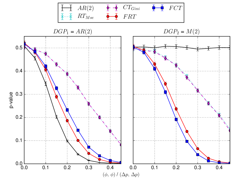
Figure 3: P-values of all models when predicting an autoregressive process $\textrm{AR}(2)$ and a binary Markov process $\textrm{M}(2)$ as function of the parameters $\left(\phi_{1},\,\phi_{2}=\phi_{1}\right)$ and $\left(\Delta p_{1},\,\Delta p_{2}=\Delta p_{1}\right)$. The prediction is made for sample size $T=500$ and calibration window length $L=50$. The regression tree with MSE loss and the classification tree with Gini index loss perform similarly on both DGPs, but have the lowest performance on the autoregressive processes. The fixed regression and classification tree perform almost identically on both DGPs. The autoregressive process is optimal at predicting itself, however fails entirely at predicting the binary Markov process. The fixed trees exhibit a small bias at $\phi=0$ resulting from the effect described in Appendix A.

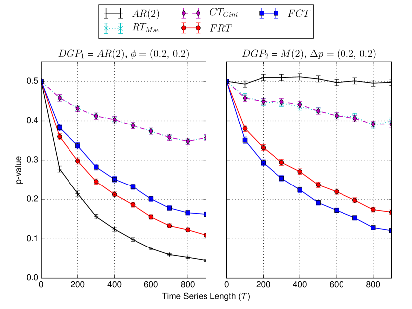
Figure 4: P-values of all models with calibration length $L=50$ when predicting an autoregressive process $\textrm{AR}(2)$ and binary Markov process $\textrm{M}(2)$, with parameters $\left(\phi_{1}=0.2,\,\phi_{2}=0.2\right)$, respectively $\left(\Delta p_{1}=0.2,\,\Delta p_{2}=0.2\right)$. The significance of the performance increases with the sample size $T$. The tree based models performs similarly on both DGPs. The autoregressive predictor only work on the autoregressive DGP.

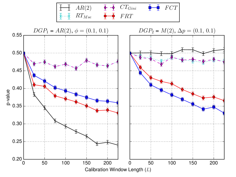
Figure 5: P-values of all models for sample size $T=500$ when predicting an autoregressive process $\textrm{AR}(2)$ and binary Markov process $\textrm{M}(2)$, with parameters $\left(\phi_{1}=0.1,\,\phi_{2}=0.1\right)$, respectively $\left(\Delta p_{1}=0.1,\,\Delta p_{2}=0.1\right)$. The significance of the predictability increases with the calibration window length $L$ as the estimation of the parameters becomes more robust.

6 Empirical Results

6.1 Data & Parameters

To demonstrate how decision tree based models can outperform autoregressive models on real data, we analyze the forecasting performance of all strategies on daily returns of the S&P 500 during the 20 year time period Jan. 1, 1995 to Dec. 31, 2015. The daily returns are obtained from Thomson-Reuters Eikon with dividend adjustment. The studied universe of strategies arises from the models in Table 1, backtested for all calibration window lengths $L\in\left\{10,\,20,\,\ldots,\,500\right\}$ and lags $\varrho\in\left\{1,\,2,\,3,\,4\right\}$.

Two strategies that only differ by their calibration window lengths $L_{1}$ and $L_{2}$ are highly correlated when $\left|L_{2}-L_{1}\right|<10$. A step size of $\Delta L=10$ allows us to find the optimal length with sufficient accuracy, while avoiding to compare almost identical strategies. We remark that the bootstrap algorithm maintains the correlation structure, and therefore the multiple testing adjusted p-values are not impacted by the choice of $\Delta L$. The upper bound of 500 trading days on $L$ results from the fact that the best strategies were found well below this bound.

The limit $\varrho\leq 4$ on the number of lags $\varrho$ arises from the condition $\frac{L}{2^{\varrho}}\geq 20$, which imposes the lower bound of $20$ on the an average samples per leaf in a decision tree, or equivalently a $\approx 5\%$ accuracy on the class probabilities. At lag $\varrho=5$, the class probabilities would be determined with a $6.5\%$ accuracy, which is too high for a meaningful prediction.

To perform the bandwidth selection for the HAC covariance matrix estimation, as well as the bootstrap block size selection, we chose the parametric $\textrm{AR}(\varrho)-\textrm{GARCH}\left(\varrho,\,\varrho\right)$ model. The model parameters are obtained by regression on the daily returns of the S&P 500 on the entire time period. The optimal parameters, determined by simulation, were found to have a kernel bandwidth $S_{5000}^{*}=2.7$ and block size $b=5$, roughly independent of the lag $\varrho$.

6.2 Performance of the Top Strategies

The individual p-values of all 1000 strategies are shown in Figure 6. The individual p-values are shown instead of the multiple testing adjusted p-values because in the later most p-values are simply one, and the relative performance is not visible anymore. The best performing predictor is the fixed classification tree ($FCT$) with lags $\varrho=2$ and calibration length $L=370$, which had a studentized Sharpe ratio performance of $\Delta_{S}^{1st}=2.12$, noticeably higher then the second best predictor at $\Delta_{S}^{2nd}=2.05$. This predictor was found to have a performance above the 99% confidence level when adjusting for multiple testing of all 1000 strategies. The fixed classification and regression trees are the only predictors that reach a performance above the 95% confidence level for a large range of lags and calibration lengths, when adjusted for multiple testing. This thick set of outperforming rules shows the presence of a robust signal, which has low probability of being a spurious phenomenon due to data-snooping. At lag $\varrho=4$, the length $L$ is to small for a robust calibration length and no predictor reaches significant results. This confirms the choice of tested lags. The results are in line with the simulation where the fixed trees were the most robust predictors, and longer calibration length provide a more robust parameter estimation.

The cumulative returns over time for the buy-and-hold strategy and the best fixed classification tree predictors are shown in Figure 7 without and with typical transaction costs. The one-way transaction costs of 0.05% applied at each buy or sell is supported by the discussion of Hsu et al. (2010, sec. 4.2). The strongest predictability arises during the burst of the dotcom bubble, the crash of the financial crisis, and the European debt crisis. Some performance metrics for the best strategy in each model class are shown in Table 2. The best strategy achieves twice the buy-and-hold return, twice the Sharpe ratio, and roughly a third of the maximum draw down. The break even costs of 21.4 bps per round trip are higher then the typical 10 bps of costs on actual markets .

6.3 Further Analysis

The statistical significance of the best performing strategies does not imply that the EMH is violated, as it may have been impossible to select one of these strategies ex-ante. Following the EMH definition of Timmermann and Granger (2004), there needs to be a search technology that would have selected the winning strategy. To test for the EMH, we use the search technology that invests at every point in time into the strategy with the best Sharpe ratio after 10bps of round trip transaction costs. The search technology uses an expanding window over all past returns. As can be seen in the lower plot of Figure 7, the FCT strategy with lag $\varrho=1$ and $L=340$ starts to outperform the two next best strategies early on around 1997. The search technology confirms that no other strategy in our universe of 1000 strategies would have hindered the ex-ante generation of economic profits in excess of the buy-and-hold strategy. Consequently, our result does seem to violate the EMH, or at least raises questions about what limits to arbitrage could have prevented the implementation of such strategies, at least in the last two decades. The test period, which includes two major crashes, is unlikely to hide extreme events that could drastically change the downside risks of the strategy with respect to the market. We believe that our test shows excess economic profits after realistic risk adjustments. However, an accurate simulation of transaction costs and potential market friction would have to be performed to confirm the result.

To determine if this abnormal performance can be explained by known factors, we evaluate the performance with the CAPM, the three-factor model of Fama and French (1993), and the four-factor model of Carhart (1997). The full four-factor model measures performance as a time-series regression of

$$r_{t}-r_{t}^{f}=\alpha+\beta_{MKT}\left(r_{t}^{MKT}-r_{t}^{f}\right)+\beta_{SMB}SMB_{t}+\beta_{HML}HML_{t}+\beta_{MOM}MOM_{t}+e_{t}.$$ (30)

In this regression, $r_{t}$ is the strategy return on month $t$, $r_{t}^{f}$ is the risk-free rate (the 1-month U.S. Treasury bill rate), $r_{t}^{MKT}$ is the market return, $SMB_{t}$ and $HML_{t}$ are the size and value-growth returns of Fama and French (1993), $MOM_{t}$ is the momentum return, $\alpha$ is the average return not explained by the benchmark model, and $e_{t}$ the residual error term. The values for $r_{t}^{f}$, $r_{t}^{MKT}$, $SMB_{t}$, $HML_{t}$ and $MOM_{t}$ are taken from Ken French’s data library (French, 2012), and derive from underlying stock returns data from the Center for Research in Security Prices (CRSP). The three-factor model is obtained by leaving out the momentum term, and the CAPM is obtained by further leaving out the $SMB$ and $HML$ factors. Table 3 shows the intercept and regression slopes (load) for all three models, including their t-statistics. The returns of the three best strategies are partially explained by the market returns (significant $\beta_{MKT}$), but nevertheless all three have significant intercept $\alpha$ that remains unexplained by known factors. The return sign correlation uncovered by the decision tree strategies qualifies as a new anomalous factor.

To obtain a better understanding of the return dynamics that generate the predictability during the burst of the different bubbles, we present in Figure 8 a zoom-in on this periods. During each period, the best performing strategy is significant at the 99.9% level when performing a bootstrap of returns under the stationarity condition (see Section 4.3). The burst of the dotcom bubble is dominated by a predictable return sign pattern at lag two (break-even cost of 45 bps per round trip). The crash of the financial crisis is dominated by a one day return sign dependency (break-even cost of 83 bps per round trip). Finally, the European debt crisis exhibits a more intricate three lag pattern that cannot be captured by lower lag strategies (break-even cost of 32 bps per round trip). The abnormal transition probabilities of these patterns are presented in Table 4. These stationary snapshots over the whole duration of each bubble confirm the significant directional accuracy.

Applying the theoretical model developed in Section 3.2 and 3.3, to the stationary snapshots of the three periods of abnormal returns, confirms the fundamental concept that autoregressive models poorly capture return sign correlations. The expected autoregressive parameters computed with Equation (18) based on the values of Table 4 are

$$E_{\textrm{Dotcom}}\left[\phi\right] =\left(0.006,\,-0.013\right),$$

$$E_{\textrm{Financial Crisis}}\left[\phi\right] =\left(-0.027\right),\,\textrm{and}$$

$$E_{\textrm{European Debt Crisis}}\left[\phi\right] =\left(-0.000,\,0.008,\,0.013\right).$$

The expected parameters $\phi$ have been scaled so as to be comparable with the directional accuracies presented in Table 4. The values show that the autoregressive model captures at most 2.7% of excess directional accuracy, far smaller then the maximal 17% of directional accuracy capture by the fixed classification tree. Hence, the theoretical model explains why the autoregressive underperforms the fixed trees on the S&P 500 as shown by Figure 6.

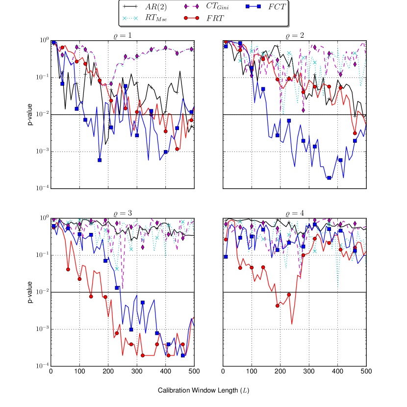
Figure 6: Overview of the individual p-values of all strategies on the S&P 500 during the 20 year time period Jan. 1, 1995 to Dec. 31, 2015. The five forecasting models are: autoregressive ($AR$); regression and classification tree ($RT_{MSE}$, $CT_{Gini}$); and the fixed regression and classification trees ($FRT$, $FCT$). Each forecasting model is run for the lags $\varrho=\left\{1,\,2,\,3,\,4\right\}$ and calibration window lengths $L=\left\{10,\,20,\,\ldots,\,500\right\}$. The p-values are obtained by 5000 bootstrap simulations. The fixed trees perform above the 95% confidence level at lags $\left\{1,\,2,\,3\right\}$ and calibration window length $\varrho\geq 250$. The other models never perform significantly.

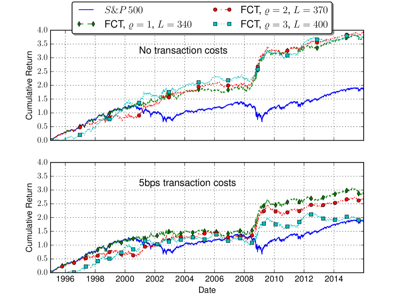
Figure 7: Cumulative returns without (upper plot) and with (lower plot) transaction costs of the top performing model ($FCT$) at three different lags on the S&P 500 during the 20 year time period Jan. 1, 1995 to Dec. 31, 2015. The highest predictability arises during the crash of the financial crisis in 2008 for all lags. Noticeable predictability arises as well during the implosion of the dotcom bubble from 2000 to 2003 at lag $p=2$ and during the European debt crisis in late 2011 at lag $p=3$. The lower plot shows the same strategies with 10bps of round trip transaction costs.

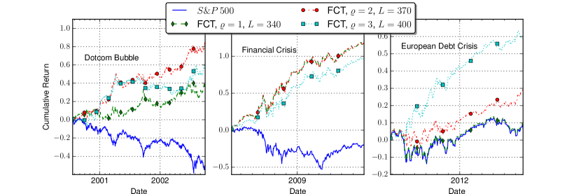
Figure 8: Cumulative returns without transaction costs of the top performing model ($FCT$) at three different lags on the S&P 500 during the anomalous periods. The left plot shows the anomalous performance of the fixed classification tree with lag $\varrho=2$ and calibration length $L=340$ during the burst of the dotcom bubble. The center plot shows the anomalous performance of the fixed classification tree with lag $\varrho=1$ and calibration length $L=370$ during the financial crisis. The right plot shows the anomalous performance of the fixed classification tree with lag $\varrho=3$ and calibration length $L=400$ during the European debt crisis.

Model	$\varrho$	$L$	$r_{y}$(%)	$Sh_{y}$	MD (%)	$\rho$	$\rho^{adj}$	BE (bps)	#RT
B&H			5.15	0.49	-30.5			0	0
FCT	2	370	7.87	0.96	-12.2	$<2.0\cdot 10^{-4}$	$0.004$	16.4	1246
FCT	3	400	7.80	0.94	-10.1	$<2.0\cdot 10^{-4}$	$0.031$	10.6	1870
FCT	1	340	7.65	0.86	-10.6	$\leq 5.9\cdot 10^{-4}$	$0.031$	21.4	860
FRT	3	330	7.86	0.92	-12.6	$<2.0\cdot 10^{-4}$	$0.043$	8.3	2417
AR	1	200	6.15	0.53	-23.4	$0.002$	$0.750$	2.2	2728
$RT_{MSE}$	2	210	5.75	0.55	-13.7	$0.010$	$0.920$	1.3	2653
$CT_{Gini}$	3	250	5.58	0.88	-15.4	$0.012$	$0.953$	0.9	2651

Table 2: Summary of the top performing strategies. The key values in order are: the model family; the number of lags $\varrho$; the calibration window length $L$; the compounded annual return $r_{y}$; the yearly Sharpe ratio $Sh_{y}$; the maximum draw down MD; the individual p-value; the p-value adjusted for multiple-testing in the entire universe of models; the break-even transaction costs (BE) with the buy-and-hold strategy; and the number of round trips #RT.

FCT	$\alpha\,\left(t_{{\scriptscriptstyle\alpha}}\right)$	${\scriptstyle\beta_{MKT}\,\left(t_{MKT}\right)}$	${\scriptstyle\beta_{SMB}\,\left(t_{SMB}\right)}$	${\scriptstyle\beta_{HML}\,\left(t_{HML}\right)}$	${\scriptstyle\beta_{MOM}\,\left(t_{MOM}\right)}$	$R^{2}$
$\varrho=1$	1.06 (3.5)	0.31 (4.7)				0.08
$L=340$	1.03 (3.4)	0.31 (4.5)	0.10 (1.1)	0.10 (1.0)		0.09
	0.90 (2.9)	0.38 (5.2)	0.08 (0.8)	0.16 (1.6)	0.16 (2.7)	0.11
$\varrho=2$	1.22 (4.2)	0.20 (3.1)				0.04
$L=370$	1.20 (4.1)	0.19 (2.9)	0.07 (0.8)	0.04 (0.4)		0.04
	1.21 (4.1)	0.19 (2.6)	0.08 (0.8)	0.03 (0.3)	-0.02 (-0.3)	0.04
$\varrho=3$	1.19 (3.7)	0.20 (2.7)				0.03
$L=400$	1.20 (3.7)	0.16 (2.2)	0.13 (1.2)	-0.07 (-0.7)		0.04
	1.17 (3.5)	0.18 (2.2)	0.12 (1.2)	-0.06 (-0.6)	0.04 (0.5)	0.04

Table 3: Intercepts and slopes in variants of regression for the three top performing FCT strategies on the S&P 500. The table shows the monthly intercepts ($\alpha$) and regression slopes ($\beta_{MKT}$, $\beta_{SMB}$, $\beta_{HML}$ and $\beta_{MOM}$, for $r^{MKT}-r^{f}$, $SMB$, $HML$, and $MOM$, respectively), as well as their t-statistics, for the CAPM, three-factor, and four-factor versions of regression. The factors are estimated for the three top performing FCTs on the S&P 500 between Jan. 1, 1995 and Dec. 31 2015 at zero transaction cost, as shown in Figure 7. The monthly intercepts are significant for all strategies and regression models. As well the market factor is significant in all cases, and particularly strongly at lag $\varrho=1$. The FCT with lag one correlates significantly with momentum.

Dotcom Bubble		Financial Crisis		European Debt Crisis
$P\left(+\right)\approx 0.48$		$P\left(+\right)\approx 0.52$		$P\left(+\right)\approx 0.56$
$P\left(--\rightarrow+\right)$	$\approx 0.54$	$P\left(-\rightarrow+\right)$	$\approx 0.61$	$P\left(---\rightarrow+\right)$	$\approx 0.56$
$P\left(-+\rightarrow-\right)$	$\approx 0.53$	$P\left(+\rightarrow-\right)$	$\approx 0.55$	$P\left(--+\rightarrow+\right)$	$\approx 0.59$
$P\left(+-\rightarrow-\right)$	$\approx 0.54$			$P\left(-+-\rightarrow-\right)$	$\approx 0.50$
$P\left(++\rightarrow-\right)$	$\approx 0.56$			$P\left(+--\rightarrow-\right)$	$\approx 0.56$
				$P\left(-++\rightarrow+\right)$	$\approx 0.67$
				$P\left(+-+\rightarrow+\right)$	$\approx 0.60$
				$P\left(++-\rightarrow+\right)$	$\approx 0.67$
				$P\left(+++\rightarrow-\right)$	$\approx 0.55$

Table 4: Daily return sign correlations of the S&P 500 during the burst of the dotcom bubble, financial crisis, and European debt crisis. The sign correlations are computed based the whole time periods shown in Figure 8, and do not account for potential non-stationarity. The burst of the dotcom bubble had more down moves then up moves, with significant two day directional accuracy. The crash of the financial crisis is impregnated by a daily reversal of the return sign, with up moves being 11% more likely then down moves after a down move. The European debt crisis exhibits a more intricate three day sign correlation, with an up move being 10 to 17% more likely then a down move after two up moves and one down move in arbitrary order.

7 Conclusion

The EMH is an assumption about financial market at the heart of many regulatory decisions. This hypothesis has been verified to hold true for a large range of regressive forecasting models, technical trading rules and asset portfolios. However, recent developments in statistical learning have not yet undergone a rigorous test.

In this paper, we presented a common non linearly separable pattern that can arise, but cannot be forecast using autoregressive models. Decision tree models possess arbitrary flexibility and are well suited to capture these non linearly separable patterns. The issue of overfitting can be addressed with an adequate lower bound on the number of samples per leaf in a decision tree. We provide a connection between fixed decision trees and Markov chains. The presented class of binary Markov processes with a deterministic component are proven to be unpredictable with autoregressive models. In contrast, the fixed classification trees only marginally underperform an autoregressive forecast on an autoregressive DGP for most parameter choices. A simulation study confirmed the theoretical results and the robustness of fixed classification and regression trees.

The models are tested on daily returns of the S&P 500 for different lags and calibration window lengths, giving rise to a universe of 1000 strategies. The multiple testing adjusted p-value of each strategy, benchmarked against the buy-and-hold strategy, is computed using the methodology of Romano and Wolf (2005) and Ledoit and Wolf (2008). The fixed classification tree (FCT) at lags $\varrho\in\left\{1,\,2,\,3\right\}$ and calibration window length $L\in\left[300,\,460\right]$ are the best strategies, significant above the 95% confidence level. This confirms the simulation results where the fixed trees were robust predictors for autoregressive and Markov based processes. The analysis showed that the theoretical model holds true on the S&P 500 to explain the performance difference between decision trees and autoregressive strategies.

Without transaction costs, the best fixed tree strategies more then double the cumulative return and Sharpe ratio of the buy-and-hold strategy. They break even with the buy-and-hold strategy at transaction costs as high as 21 bps per round trip. A simple best Sharpe ratio search technology could have selected ex-ante the best performing strategy. The strategies all have significant intercept for the four-factor regression model. Therefore, the EMH appears to be violated, in particular during the dotcom bubble (2000-2003), the financial crisis (2008-2009) and the European debt crisis (2012). During bull markets, the performance of decision tree based strategies is roughly equal to the buy-and-hold strategy. While no certain explanation can be given, it would not be surprising to find that behavioral heuristics, as exposed by Tversky and Kahneman (1974) even among trained statisticians, have significant impact during a market crash. The strong return sign correlations speak in favor of biases in human heuristics relying more on past return signs then on the amplitude.

The finding of this study stands in contrast with multiple prior market efficiency studies that included the S&P 500. The studies by Sullivan et al. (1999); Hsu and Kuan (2005) found no significantly performing technical trading rule on the S&P 500, while our fixed classification trees perform significantly on a longer test period of 20 years. The study by Hsu et al. (2010), as well testing technical trading rules, further concluded that market efficiency has increased after the introduction of ETFs in the year 2000, and that emerging markets are less efficient then more mature markets. Our study provides a solid counter example of a mature market that exhibits large inefficiencies. As well, the largest inefficiencies appear long after the introduction of ETFs, casting doubt on the impact of ETFs on market efficiency. The discrepancy with prior studies is a result of their focus on technical trading rules. Our work shows that market efficiency cannot be measured only using technical trading rules.

Noticeable research has gone into detecting explosive regimes in stock markets (Phillips et al., 2011; Kaizoji et al., 2015; Sornette and Cauwels, 2015), and studying the growth phase of bubbles. In contrast, the return dynamics during the burst of a bubble seem under researched as shown by the recent findings of an acceleration factor (Ardila et al., 2015) and the novel return sign predictability established in this paper. Future research needs to study more in detail the predictability dynamics during bubbles on other stock indices. As well, it needs to be better understood which stocks in an equity drive the predictability.

Funding

This work was supported by ETH Zürich under Grant [number 0-20029-14].

Appendix A P-value Bias

The p-values arising for certain metrics from simple prediction strategies can exhibit non-intuitive biases. For example, let us consider the strategy with signal

$$s_{t+1}=\textrm{sign}\left(r_{t}\right),$$ (31)

which predicts for each time step the sign of the previous return. We benchmark this strategy against the buy-and-hold strategy $s_{t+1}^{BH}=1$ using the mean return as a performance metric. When predicting two returns $\left(r_{0},\,r_{1},\,r_{2}\right)$, where $r_{0}$ is a dummy return needed for the prediction, the mean return difference between the two strategies is

$$\Delta\bar{r}=\underbrace{\frac{1}{2}\left(\textrm{sign}\left(r_{0}\right)r_{1}+\textrm{sign}\left(r_{1}\right)r_{2}\right)}_{\textrm{strategy}}-\underbrace{\frac{1}{2}\left(r_{1}+r_{2}\right)}_{\textrm{buy-and-hold}}.$$ (32)

While the expected mean return difference is zero, $E\left[\Delta\bar{r}\right]=0$, the probabilities of it being positive or negative are not symmetric. To show that $p\left(\Delta\bar{r}>0\right)\neq p\left(\Delta\bar{r}<0\right),$ we compute the value for all possible scenarios in Table 5, and can determine the probabilities to almost surely be

$$p\left(\Delta\bar{r}>0\right)=\frac{5}{16},\,p\left(\Delta\bar{r}=0\right)=\frac{4}{16}\;\textrm{and}\;p\left(\Delta\bar{r}<0\right)=\frac{7}{16}.$$ (33)

The p-value associated to the strategy outperforming the benchmark would be $p\left(\Delta\bar{r}<0\right)+\frac{1}{2}p\left(\Delta\bar{r}=0\right)=\frac{7}{16}+\frac{1}{2}\cdot\frac{4}{16}=0.5625$. This bias decreases with the number of predicted returns as shown in Figure 9. The bias decays with the sample size $T$, but remains significant for the sample sizes of interest.

$\textrm{sign}\left(r_{0},\,r_{1},\,r_{2}\right)$	$\Delta\bar{r}$
$\left(+,\,+,\,+\right)$	$r_{1}+r_{2}-r_{1}-r_{2}=0$
$\left(+,\,+,\,-\right)$	$r_{1}+r_{2}-r_{1}-r_{2}=0$
$\left(+,\,-,\,+\right)$	$\frac{1}{2}\left(r_{1}-r_{2}-r_{1}-r_{2}\right)=\boldsymbol{-r_{2}\leq 0}$
$\left(+,\,-,\,-\right)$	$\frac{1}{2}\left(r_{1}-r_{2}-r_{1}-r_{2}\right)=-r_{2}\geq 0$
$\left(-,\,-,\,-\right)$	$\frac{1}{2}\left(-r_{1}-r_{2}-r_{1}-r_{2}\right)=-r_{1}-r_{2}\geq 0$
$\left(-,\,-,\,+\right)$	$\frac{1}{2}\left(-r_{1}-r_{2}-r_{1}-r_{2}\right)=-r_{1}-r_{2}\sim 0$
$\left(-,\,+,\,-\right)$	$\frac{1}{2}\left(-r_{1}+r_{2}-r_{1}-r_{2}\right)=\boldsymbol{-r_{1}\leq 0}$
$\left(-,\,+,\,+\right)$	$\frac{1}{2}\left(-r_{1}+r_{2}-r_{1}-r_{2}\right)=\boldsymbol{-r_{1}\leq 0}$

Table 5: Mean return difference between the buy-and-hold and previous sign prediction strategies. The table lists all cases predicting two returns $r_{1}$ and $r_{2}$.

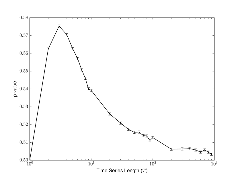
Figure 9: P-value of the mean return metric for the previous sign prediction strategy as a function of the sample size $T$. As computed in Equation 33, the p-value is exactly $\rho=0.5625$ for $T=2$. The bias decays with the sample length, but remains significant above 0.5% at sample length $T$.

References

- Andersen and Sornette (2005) Andersen, J.V. and Sornette, D., A Mechanism for Pockets of Predictability in Complex Adaptive Systems. Europhys. Lett., 2005, 70, 697–703.
- Andrews (1991) Andrews, D., Heteroskedasticity and Autocorrelation Consistent Covariance Matrix Estimation. Econometrica, 1991, 59, 817–858.
- Ardila et al. (2015) Ardila, D.A., Forro, Z. and Sornette, D., The Acceleration Effect and Gamma Factor in Asset Pricing. Swiss Finance Institute Research Paper No. 15-30. Available at SSRN: http://ssrn.com/abstract=2645882, 2015.
- Barras et al. (2005) Barras, L., Scaillet, O. and Wermers, R., False Discoveries in Mutual Fund Performance : Measuring Luck in Estimated Alphas. The Journal of Finance, 2005, 65, 179–216.
- Carhart (1997) Carhart, M.M., On Persistence in Mutual Fund Performance. The Journal of Finance, 1997, 52, 57–82.
- Christoffersen and Diebold (2003) Christoffersen, P.F. and Diebold, F.X., Financial Asset Returns, Direction-of-Change Forecasting, and Volatility Dynamics. Management Science, 2003, 52, 1273–1287.
- Christoffersen et al. (2006) Christoffersen, P.F., Diebold, F.X., Mariano, R.S., Tay, A.S. and Tse, Y.K., Direction-of-Change Forecasts Based on Conditional Variance, Skewness and Kurtosis Dynamics: International Evidence. Journal of Financial Forecasting, 2006, 1, 1–22.
- Cont (2001) Cont, R., Empirical properties of asset returns: stylized facts and statistical issues. Quantitative Finance, 2001, 1, 223–236.
- Fama (1970) Fama, E.F., Efficient Capital Markets: A Review of Theory and Empirical Work. The Journal of Finance, 1970, 25, 383–417.
- Fama (1991) Fama, E.F., Efficient Capital Markets: II. The Journal of Finance, 1991, 46, 1575–1617.
- Fama and French (1993) Fama, E.F. and French, K.R., Common risk factors in the returns on stocks and bonds. Journal of Financial Economics, 1993, 33, 3–56.
- Fama and French (2009) Fama, E.F. and French, K.R., Luck Versus Skill in the Cross Section of Mutual Fund Return. Journal of Finance, 2009, 65, 1915–1947.
- French (2012) French, K., Data Library. , 2012.
- Grossman and Stiglitz (1980) Grossman, S.J. and Stiglitz, J.E., On the impossibility of informationally efficient markets. The American Economic Review, 1980, 70, 293–408.
- Hamilton (1994) Hamilton, J.D., Time Series Analysis, 1 , 1994, Princeton University Press.
- Harras and Sornette (2011) Harras, G. and Sornette, D., How to grow a bubble: A model of myopic adapting agents. Journal of Economic Behavior and Organization, 2011, 80, 137–152.
- Hastie et al. (2001) Hastie, T., Tibshirani, R. and Friedman, J., The Elements of Statistical Learning, Springer Series in Statistics Vol. 1, , 2001 (Springer New York Inc.: New York, NY, USA).
- Hsu et al. (2010) Hsu, P.H., Hsu, Y.C. and Kuan, C.M., Testing the predictive ability of technical analysis using a new stepwise test without data snooping bias. Journal of Empirical Finance, 2010, 17, 471–484.
- Hsu and Kuan (2005) Hsu, P.H. and Kuan, C.M., Reexamining the Profitability of Technical Analysis with Data Snooping Checks. Journal of Financial Econometrics, 2005, 3, 606–628.
- Hsu et al. (2016) Hsu, P.H., Taylor, M.P. and Wang, Z., Technical trading: Is it still beating the foreign exchange market?. Journal of International Economics, 2016, 102, 188–208.
- Hyafil and Rivest (1976) Hyafil, L. and Rivest, R.L., Constructing optimal binary decision trees is NP-complete. Information Processing Letters, 1976, 5, 15–17.
- James et al. (2014) James, G., Witten, D., Hastie, T. and Tibshirani, R., An Introduction to Statistical Learning: With Applications in R, 2014, Springer Publishing Company, Incorporated.
- Johansen et al. (2000) Johansen, A., Ledoit, O. and Sornette, D., Crashes as critical points. International Journal of Theoretical and Applied Finance, 2000, 3, 219–255.
- Kaizoji et al. (2015) Kaizoji, T., Leiss, M., Saichev, A. and Sornette, D., Super-exponential endogenous bubbles in an equilibrium model of rational and noise traders. Journal of Economic Behavior and Organization, 2015, 112, 289–310.
- Ledoit and Wolf (2008) Ledoit, O. and Wolf, M., Robust Performance Hypothesis Testing with the Sharpe Ratio. Journal of Empirical Finance, 2008, 15, 850–859.
- Leung et al. (2000) Leung, M.T., Daouk, H. and Chen, A.S., Forecasting stock indices: a comparison of classification and level estimation models. International Journal of Forecasting, 2000, 16, 173–190.
- Malkiel (2003) Malkiel, B.G., The Efficient Market Hypothesis and Its Critics. Journal of Economic Perspectives, 2003, 17, 59–82.
- Mills and Markellos (2008) Mills, T.C. and Markellos, R.N., The Econometric Modelling of Financial Time Series, 2008, Cambridge University Press.
- Mills and Markellos (2009) Mills, T.C. and Markellos, R.N., Financial Economics, Non-linear Time Series in. In Encyclopedia of Complexity and Systems Science, pp. 3435–3448, 2009.
- Newey and West (1994) Newey, W.K. and West, K., Automatic Lag Selection in Covariance Matrix Estimation. Review of Economic Studies, 1994, 61, 631–653.
- Niederhoffer and Osborne (1966) Niederhoffer, V. and Osborne, M.F.M., Market Making and Reversal on the Stock Exchange. Journal of the American Statistical Association, 1966, 61, 897–916.
- Pedregosa et al. (2011) Pedregosa, F., Varoquaux, G., Gramfort, A., Michel, V., Thirion, B., Grisel, O., Blondel, M., Prettenhofer, P., Weiss, R., Dubourg, V., Vanderplas, J., Passos, A., Cournapeau, D., Brucher, M., Perrot, M. and Duchesnay, E., Scikit-learn: Machine Learning in Python. Journal of Machine Learning Research, 2011, 12, 2825–2830.
- Phillips et al. (2011) Phillips, P.C.B., Wu, Y. and Yu, J., Explosive behavior in the 1990s Nasdaq: When did exuberance escalate asset values?. International Economic Review, 2011, 52, 201–226.
- Politis and Romano (1992) Politis, D.N. and Romano, J.P., A circular block-resampling procedure for stationary data. Exploring the limits of bootstrap, 1992, pp. 263–270.
- Romano and Wolf (2005) Romano, J.P. and Wolf, M., Stepwise multiple testing as formalized data snooping. Econometrica, 2005, 73, 1237–1282.
- Romano and Wolf (2016) Romano, J.P. and Wolf, M., Efficient computation of adjusted p-values for resampling-based stepdown multiple testing. Statistics & Probability Letters, 2016, 113, 38–40.
- Satinover and Sornette (2012a) Satinover, J.B. and Sornette, D., Cycles, determinism and persistence in agent-based games and financial time-series I. Quantitative Finance, 2012a, 12, 1051–1064.
- Satinover and Sornette (2012b) Satinover, J.B. and Sornette, D., Cycles, determinism and persistence in agent-based games and financial time-series II. Quantitative Finance, 2012b, 12, 1064–1078.
- Sornette (2003) Sornette, D., Why Stock Markets Crash: Critical Events in Complex Financial Systems, 2003, Princeton University Press.
- Sornette and Cauwels (2015) Sornette, D. and Cauwels, P., Financial bubbles: mechanisms and diagnostics. Review of Behavioral Economics, 2015, 2, 279–305.
- Sullivan et al. (1999) Sullivan, R., Timmermann, A. and White, H., Data-Snooping, Technical Trading Rule Performance, and the Bootstrap. The Journal of Finance, 1999, 54, 1647–1691.
- Timmermann and Granger (2004) Timmermann, A. and Granger, C.W.J., Efficient market hypothesis and forecasting. International Journal of Forecasting, 2004, 20, 15–27.
- Tversky and Kahneman (1974) Tversky, A. and Kahneman, D., Judgment under Uncertainty: Heuristics and Biases. Science, 1974, 185, 1124–1131.
- White (2000) White, H., A Reality Check for Data Snooping. Econometrica, 2000, 68, 1097–1126.
- Yen et al. (2015) Yen, S.M.F., Hsu, Y.L. and Hsiao, Y.L., Can hedge fund elites consistently beat the benchmark? A study of portfolio optimization. Asia Pacific Management Review, 2015, 20, 275–284.
- Zhang (1999) Zhang, Y.c., Toward a theory of marginally efficient markets. Physica A: Statistical Mechanics and its Applications, 1999, 269, 30–44.
- Zunino et al. (2009) Zunino, L., Zanin, M., Tabak, B.M., Pérez, D.G. and Rosso, O.A., Forbidden patterns, permutation entropy and stock market inefficiency. Physica A: Statistical Mechanics and its Applications, 2009, 388, 2854–2864.