Towards a Theoretical Analysis of PCA for Heteroscedastic Data

Abstract

Principal Component Analysis (PCA) is a method for estimating a subspace given noisy samples. It is useful in a variety of problems ranging from dimensionality reduction to anomaly detection and the visualization of high dimensional data. PCA performs well in the presence of moderate noise and even with missing data, but is also sensitive to outliers. PCA is also known to have a phase transition when noise is independent and identically distributed; recovery of the subspace sharply declines at a threshold noise variance. Effective use of PCA requires a rigorous understanding of these behaviors. This paper provides a step towards an analysis of PCA for samples with heteroscedastic noise, that is, samples that have non-uniform noise variances and so are no longer identically distributed. In particular, we provide a simple asymptotic prediction of the recovery of a one-dimensional subspace from noisy heteroscedastic samples. The prediction enables: a) easy and efficient calculation of the asymptotic performance, and b) qualitative reasoning to understand how PCA is impacted by heteroscedasticity (such as outliers).

I Introduction

Given noisy measurements of points from a subspace, one may estimate the subspace with Principal Component Analysis (PCA). Estimating a $k$-dimensional subspace from noisy samples $y_{1},\dots,y_{n}\in\mathbb{R}^{d}$ by PCA is accomplished by solving the non-convex problem

$$\hat{U}=\operatorname*{argmin}_{U\in\mathbb{R}^{d\times k}:U^{T}U=I}\min_{z_{i}\in\mathbb{R}^{k}}\sum_{i=1}^{n}\|y_{i}-Uz_{i}\|_{2}^{2},$$ (1)

which can be done efficiently via the singular value decomposition. PCA performs well in the presence of low to moderate noise and even performs well with missing data [1, 2]. Furthermore, for mean zero data, representing the samples in the basis produced by PCA gives coordinates that are uncorrelated and provide a convenient representation of the data where the relevant factors have been decoupled.

As a result of such nice properties, PCA has been applied in myriad contexts to accomplish tasks such as dimensionality reduction, anomaly detection and the visualization of high dimensional data. A small sample of these settings include medical imaging [3], anomaly detection on computer networks [4] and dimensionality reduction for classification [5]. It has also been used to model images taken of a scene under various illuminations [6] as well as measurements taken in environmental monitoring [7, 8], to name just a few.

To use PCA effectively in all these settings, it is important to rigorously understand its performance under a variety of conditions. It is known, for example, that PCA is sensitive to outliers (i.e., gross errors) [9]. Thus for problems such as computer vision modeling [10] or foreground-background separation [11] where outliers may be expected (or even of interest), robust variants [1] are used instead. PCA with independent identically distributed noise is also known to exhibit a phase transition; recovery of the subspace sharply declines after the noise variance exceeds a threshold [12].

This paper provides a step towards extending such analysis to the case where noise is heteroscedastic, that is, the case where samples have non-uniform noise variances and so are no longer identically distributed. In particular, we provide a simple asymptotic prediction of the recovery of a one-dimensional subspace from noisy heteroscedastic samples. Forming the prediction involves connecting several results from random matrix theory to obtain an initial complicated asymptotic prediction and then exploiting its structure to find a much simpler algebraic description.

The simple form enables: a) easy and efficient calculation of the asymptotic prediction, and b) reasoning qualitatively about the expressions to understand the asymptotic behavior of PCA with heteroscedastic noise. We demonstrate these benefits through an example calculation and a qualitative analysis that explains a surprising phenomenon: the largest noise variance seems to most heavily influence performance. We also perform numerical experiments to illustrate how the asymptotic prediction applies for particular (finite) choices of ambient dimension and number of samples.

The rest of the paper is organized as follows. Section II describes the model we consider (a one-dimensional signal in heteroscedastic noise) and states the main result: an asymptotic prediction for the recovery of the one-dimensional subspace by PCA. It also includes an example calculation of the asymptotic prediction for a particular set of model parameters, illustrating how the main result enables easy and efficient calculation of the prediction. Section III compares the prediction with experimental results simulated according to the model. The simulations demonstrate good agreement as the ambient dimension and number of samples grow large; when these values are small the prediction and experiment differ but have the same behavior. Section IV provides a proof of the main result. Section V uses the main result to provide a qualitative analysis of the behavior of PCA under heteroscedastic noise, revealing some interesting phenomena about the negative impact of heteroscedasticity. Finally, Section VI discusses the findings and describes avenues for future work.

II Main result

We model $n$ heteroscedastic samples $y_{1},\ldots,y_{n}\in\mathbb{R}^{d}$ from a one dimensional subspace $\tilde{u}\in\mathbb{R}^{d}$ as

$$y_{i}=\theta\tilde{u}z_{i}+\eta_{i}\varepsilon_{i}$$ (2)

where

• $\theta\in\mathbb{R}_{+}$ is the subspace amplitude,

• $\eta_{i}\in\mathbb{R}_{+}$ are the noise standard deviations,

• $\tilde{u}\in\mathbb{R}^{d}$ is the subspace and has entries $\tilde{u}_{j}\overset{\mathrm{iid}}{\sim}\mathcal{F}_{1}(0,1/d)$ with mean zero and variance $1/d$,

• $z_{i}\overset{\mathrm{iid}}{\sim}\mathcal{F}_{2}(0,1)$ are random subspace coefficients and have mean zero and unit variance, and

• $\varepsilon_{i}\in\mathbb{R}^{d}$ are independent noise vectors that have entries $\varepsilon_{ij}\overset{\mathrm{iid}}{\sim}\mathcal{F}_{3}(0,1)$ with mean zero and unit variance,

such that the distributions $\mathcal{F}_{1}$ and $\mathcal{F}_{2}$ satisfy the log-Sobolev inequality [13] and the distribution $\mathcal{F}_{3}$ satisfies condition (1.3) from [14]. Notably, these conditions are satisfied by Gaussian distributions $\mathcal{F}_{1}=\mathcal{F}_{2}=\mathcal{F}_{3}=\mathcal{N}$.

We further suppose that $L$ noise levels $\sigma_{1},\dots,\sigma_{L}$ occur in proportions $p_{1},\dots,p_{L}$. Namely, $p_{1}$ of the samples have noise level $\eta_{i}=\sigma_{1}$, $p_{2}$ have $\eta_{i}=\sigma_{2}$ and so on, where the $p_{\ell}$ values sum to unity.

The following theorem is our main result and describes how well the subspace $\tilde{u}$ is recovered by PCA as the problem dimensions grow.

Theorem 1

For fixed samples-to-dimension ratio $c>\ 1$, the PCA estimate $\hat{u}$ is such that

$$\left|\tilde{u}^{T}\hat{u}\right|^{2}\ \ \underset{{\tiny\begin{array}[]{c}n,d\rightarrow\infty\\ n/d=c\end{array}}}{\overset{a.s.}{\longrightarrow}}\max\left(0,\frac{A\left(\beta\right)}{\beta B^{\prime}\left(\beta\right)}\right)$$ (3)

where

$$A\left(x\right) =1-c\sum_{\ell=1}^{L}\frac{p_{\ell}\sigma_{\ell}^{4}}{\left(x-\sigma_{\ell}^{2}\right)^{2}}$$

$$B\left(x\right) =1-c\theta^{2}\sum_{\ell=1}^{L}\frac{p_{\ell}}{x-\sigma_{\ell}^{2}}$$

and $\beta$ is the largest real root of $B$.

Section IV presents the proof of this theorem. We illustrate Theorem 1 with the following example calculation.

Example calculation: Here we calculate the asymptotic prediction in (3) for the case:

$$c =5 p =\left(0.2,0.8\right)$$

$$\theta =2 \sigma =\left(1,2\right)$$

Namely, we determine the limit of $\left|\tilde{u}^{T}\hat{u}\right|^{2}$ when $d,n\rightarrow\infty$ for the case where there are $5$ times as many samples as the ambient dimension, the signal amplitude is $2$, and $20\%$ of the samples have low noise with variance $1$ (signal-to-noise ratio $\theta^{2}/\sigma_{1}^{2}=4$) and $80\%$ of the samples have high noise with variance $4$ (signal-to-noise ratio $\theta^{2}/\sigma_{2}^{2}=1$). The steps are as follows.

1. Substitute the values of $c,\theta,p$ and $\sigma$ into the formulas for $A$ and $B$, obtaining

   $$A\left(x\right) =1-5\cdot\left(\frac{0.2\ \cdot 1^{4}}{\left(x-1^{2}\right)^{2}}+\frac{0.8\ \cdot 2^{4}}{\left(x-2^{2}\right)^{2}}\right)$$

   $$=1-\frac{1}{\left(x-1\right)^{2}}-\frac{64}{\left(x-4\right)^{2}}$$

   $$B\left(x\right) =1-5\cdot 2^{2}\cdot\left(\frac{0.2}{x-1^{2}}+\frac{0.8}{x-2^{2}}\right)$$

   $$=1-\frac{4}{x-1}-\frac{16}{x-4}.$$

2. Find the largest root of $B$, obtaining

   $$\beta=23.466.$$

3. Evaluate $\frac{A\left(\beta\right)}{\beta B^{\prime}\left(\beta\right)},$ obtaining

   $$\frac{A\left(\beta\right)}{\beta B^{\prime}\left(\beta\right)}=0.705.$$

4. Take the maximum with zero, and conclude that

   $$\left|\tilde{u}^{T}\hat{u}\right|^{2}\ \ \underset{{\tiny\begin{array}[]{c}n,d\rightarrow\infty\\ n/d=c\end{array}}}{\overset{a.s.}{\longrightarrow}}\ \ 0.705.$$

Note that the second step can be easily done by clearing the denominator of $B$ and finding the real roots of the resulting degree $L$ polynomial (using off-the-shelf tools). Hence the asymptotic prediction can be efficiently computed.

III Experimental verification

To illustrate the main result (Theorem 1) we performed a numerical experiment for the two noise level case ($L=2$):

$$c =10 \theta =1 \sigma =(1.8,0.2)$$

where $p_{2}$ is swept from $0$ to $1$ with $p_{1}=1-p_{2}$. This allows us to investigate the accuracy of the asymptotic prediction for a variety of settings: at the extremes ($p_{2}=0,1$) the setup matches the homoscedastic setting and in the middle ($p_{2}=1/2$) the samples are split evenly between the two noise levels.

   

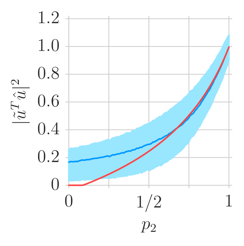
(a) Results for $d=10^{2}$ and $n=10^{3}$ ($10000$ trials).

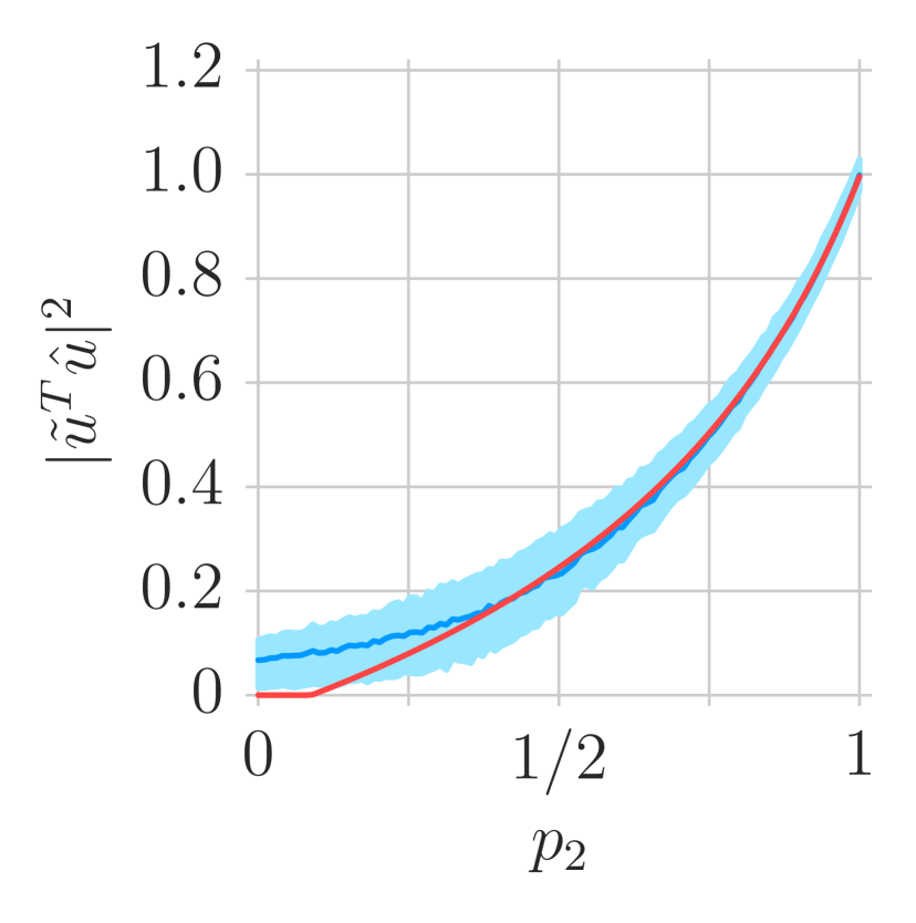
(b) Results for $d=10^{3}$ and $n=10^{4}$ ($1000$ trials).

Figure 1: Simulation results for $c=10$, $\theta=1$, $\sigma=(1.8,0.2)$ where $p_{2}$ is swept from $0$ to $1$ with $p_{1}=1-p_{2}$. Simulation mean (blue curve) and interquartile interval (light blue ribbon) shown with asymptotic prediction (red curve).

We first suppose $d=10^{2}$ and $n=10^{3}$. We performed $10000$ trials with data generated by the Gaussian distribution. Namely, $\mathcal{F}_{1}=\mathcal{F}_{2}=\mathcal{F}_{3}=\mathcal{N}$. Figure 1(a) shows the simulation results with the mean (blue curve) and interquartile interval (light blue ribbon) shown with the asymptotic prediction (red curve).

There is generally good agreement between the mean and the asymptotic prediction for $p_{2}>0.6$ (they deviate from each other by no more than $0.025$). However, the smaller the value of $p_{2}$, the greater the deviation of the prediction from the mean, with the asymptotic prediction underestimating the (non-asymptotic) simulation by at most $0.182$.

Figure 1 illustrates a general phenomenon we observed: small asymptotic predictions typically underestimate the simulation results, with smaller predictions underestimating more. Intuitively, a small prediction of this inner product corresponds to a subspace estimate that is becoming increasingly like an isotropically random vector and so it has vanishing square inner product with the true subspace as the dimension grows. Asymptotically, below the phase transition, theory predicts the subspace estimate to be practically isotropically random. However, in finite dimension there is a better chance of alignment, resulting in a positive square inner product.

We illustrate this phenomenon with a second experiment with a higher dimension of $d=10^{3}$ and a higher number of samples $n=10^{4}$ (chosen to have the same sample-to-dimension ratio $c=10$). The data were again generated using the Gaussian distribution and we performed $1000$ trials. Figure 1(b) shows the simulation results for this case. Again, the mean and interquartile interval are in blue and light blue, and the asymptotic prediction is in red. This experiment demonstrates better agreement between the mean behavior and the asymptotic prediction. In particular, for $p_{2}>0.4$ they deviate from each other by no more than $0.017$. For $p_{2}<0.4$ their largest deviation is $0.084$; notably, this is less than half of the largest deviation for the smaller experiment. Furthermore, the interquartile interval is narrower, indicating that the square inner product is concentrating.

We stress here that, while we have not proved this relationship, experimental evidence suggests that the asymptotic prediction in Theorem 1 underestimates the mean square inner product obtained in finite size experiments, and is therefore a conservative or pessimistic estimate of the performance of PCA. When determining how much to trust the subspace estimated by PCA, this conservatism might be preferable to overestimating the reliability of PCA.

Finally, note that the square inner product from the simulation is sometimes above one. This is because the true $\tilde{u}$ is a random vector and may not have unit norm. However, as the dimension grows, the norm of $\tilde{u}$ will concentrate around one (see [15] for a treatment of the concentration of the norm).

IV Proof of main result

This section proves the main result (Theorem 1). The proof has eight main parts. In IV-A, we first apply previous results in the literature to obtain an initial expression for the asymptotic prediction. This expression is difficult to evaluate and analyze because it involves an integral transform of the (nontrivial) limiting singular value distribution for a random (noise) matrix as well as the corresponding limiting largest singular value. In the remaining seven parts (IV-B-IV-H), we find a simple equivalent expression by exploiting the structure of the prediction.

IV-A Obtain an initial expression

Rewriting the model in (2) in matrix form yields

$$\mathbf{Y}:=\theta\tilde{u}z^{T}+\mathbf{E}\mathbf{H}\in\mathbb{R}^{d\times n}$$

where $\mathbf{E}\in\mathbb{R}^{d\times n}$ is a matrix with columns $\varepsilon_{1},\ldots,\varepsilon_{n}\in\mathbb{R}^{d}$ and $\mathbf{H}\in\mathbb{R}^{n\times n}$ is a diagonal matrix with diagonal entries $\eta_{1},\ldots,\eta_{n}\in\mathbb{R}$.

Recall that the subspace basis $\hat{u}$ estimated by PCA for $\mathbf{Y}$ is the first left singular vector of $\mathbf{Y}$. PCA is invariant to scaling, so $\hat{u}$ is also the first left singular vector of

$$\mathbf{\tilde{Y}}:=\frac{1}{\sqrt{n}}\mathbf{Y}.$$

The matrix $\mathbf{\tilde{Y}}$ matches the low rank (here rank one) perturbation of a random matrix model considered in [12] because

$$\mathbf{\tilde{Y}}=\mathbf{P}+\mathbf{X}$$

where

$$\mathbf{P}:=\theta\tilde{u}\left(\frac{1}{\sqrt{n}}z\right)^{T}\mathbf{X}:=\left(\frac{1}{\sqrt{n}}\mathbf{E}\right)\mathbf{H},$$

and $\mathbf{P}$ is generated according to the “i.i.d model” and satisfies Assumption 2.4 of [12], and $\mathbf{X}$ satisfies Assumptions 2.1-2.3 of [12] ($\mathbf{X}$ here matches the random matrix in [14], which [12] refers to as an example of a random matrix that satisfies the assumptions).

Thus under the condition $\varphi^{\prime}\left(b^{+}\right)=-\infty$ (we will show in subsection IV-C that it is indeed satisfied), Theorems 2.10 and 2.11 from [12] yield

$$\left|\tilde{u}^{T}\hat{u}\right|^{2}\ \ \underset{{\tiny\begin{array}[]{c}n,d\rightarrow\infty\\ n/d=c\end{array}}}{\overset{a.s.}{\longrightarrow}}\left\{\begin{array}[]{ll}\frac{-2\varphi\left(\rho\right)}{\theta^{2}D^{\prime}\left(\rho\right)}&\theta^{2}>\bar{\theta}^{2}\\ 0&\text{otherwise}\end{array}\right.$$ (4)

where

• $\rho:=D^{-1}\left(1/\theta^{2}\right)$

• $\bar{\theta}^{2}:=1/D\left(b^{+}\right)$

• $D\left(z\right):=\varphi\left(z\right)\left(c^{-1}\varphi\left(z\right)+\frac{1-c^{-1}}{z}\right)\qquad z>b$

• $\varphi\left(z\right):=\int_{a}^{b}\frac{z}{z^{2}-t^{2}}d\mu_{\mathbf{X}}\left(t\right)\qquad z>b$

• $a$ and $b$ are, respectively, the infimum and the supremum of the support of $\mu_{\mathbf{X}}$ (so $b>a\geq 0$), and

• $\mu_{\mathbf{X}}$ is the limiting singular value distribution of $\mathbf{X}$ (compactly supported by Assumption 2.1 of [12]).

We use the notation $f\left(b^{+}\right):=\lim_{z\rightarrow b^{+}}f\left(z\right)$ as a convenient shorthand for the limit of a function $f\left(z\right)$.

Evaluating this asymptotic prediction would then consist of evaluating the above intermediates from bottom to top. These steps are challenging because because they involve an integral transform of the limiting singular value distribution for the random (noise) matrix as well as the corresponding limiting largest singular value. The following sections eventually lead to the simpler expression in (3) that is easier to both evaluate and analyze.

IV-B Carry out a change of variables

We begin by introducing the function

$$\psi\left(z\right):=\frac{cz}{\varphi\left(z\right)}=\left[\frac{1}{c}\int_{a}^{b}\frac{1}{z^{2}-t^{2}}d\mu_{\mathbf{X}}\left(t\right)\right]^{-1},\ z>b$$ (5)

because it turns out to have several nice properties that simplify all of the following analysis.

Rewriting (4) using $\psi\left(z\right)$ instead of $\varphi\left(z\right)$ yields

$$\left|\tilde{u}^{T}\hat{u}\right|^{2}\ \ \underset{{\tiny\begin{array}[]{c}n,d\rightarrow\infty\\ n/d=c\end{array}}}{\overset{a.s.}{\longrightarrow}}\left\{\begin{array}[]{ll}\frac{-2c}{\theta^{2}\psi\left(\rho\right)D^{\prime}\left(\rho\right)/\rho}&\theta^{2}>\bar{\theta}^{2}\\ 0&\text{otherwise}\end{array}\right.$$

where now

$$D\left(z\right)=\frac{cz^{2}}{\left(\psi\left(z\right)\right)^{2}}+\frac{c-1}{\psi\left(z\right)},\quad z>b.$$

IV-C Find useful properties of $\psi\left(z\right)$

Establishing some properties of $\psi\left(z\right)$ aids simplification significantly. Furthermore, these properties help us show that $\varphi^{\prime}\left(b^{+}\right)$ is indeed $-\infty$, as stated above in subsection IV-A.

Property 1. We show that $\psi\left(z\right)$ satisfies a certain rational equation for all $z>b$. For this, observe that the square singular values of the noise matrix $\mathbf{X}$ are exactly the eigenvalues of $c\mathbf{X}\mathbf{X}^{T}$ divided by $c$ (since $\mathbf{X}$ has more columns than rows, namely, $c=n/d>1$). Thus we first consider the limiting eigenvalue distribution $\mu_{c\mathbf{X}\mathbf{X}^{T}}$ of $c\mathbf{X}\mathbf{X}^{T}$, and then relate its Stieltjes transform $m\left(\zeta\right)$ to $\psi\left(z\right)$.

Theorem 1 in [14] establishes that the random matrix

$$c\mathbf{X}\mathbf{X}^{T}=\left(\frac{1}{\sqrt{d}}\mathbf{E}\right)\mathbf{H}^{2}\left(\frac{1}{\sqrt{d}}\mathbf{E}\right)^{T}$$

has a limiting eigenvalue distribution $\mu_{c\mathbf{X}\mathbf{X}^{T}}$ whose Stieltjes transform

$$m\left(\zeta\right):=\int\frac{1}{t-\zeta}d\mu_{c\mathbf{X}\mathbf{X}^{T}}\left(t\right),\quad\zeta\in\mathbb{C}^{+}$$ (6)

satisfies the condition

$$\forall\zeta\in\mathbb{C}^{+}\quad m\left(\zeta\right)=-\left(\zeta-c\sum_{\ell=1}^{L}\frac{p_{\ell}\sigma_{\ell}^{2}}{1+\sigma_{\ell}^{2}m\left(\zeta\right)}\right)^{-1}$$ (7)

where $\mathbb{C}^{+}$ is the set of all complex numbers with positive imaginary part.

Since the square singular values of $\mathbf{X}$ are exactly the eigenvalues of $c\mathbf{X}\mathbf{X}^{T}$ divided by $c$, we have for all $z>b$

$$\psi\left(z\right) =\left[\frac{1}{c}\int_{a}^{b}\frac{1}{z^{2}-t^{2}}d\mu_{\mathbf{X}}\left(t\right)\right]^{-1}$$

$$=\left[\frac{1}{c}\int_{a^{2}c}^{b^{2}c}\frac{1}{z^{2}-t/c}d\mu_{c\mathbf{X}\mathbf{X}^{T}}\left(t\right)\right]^{-1}$$

$$=-\left[\int_{a^{2}c}^{b^{2}c}\frac{1}{t-z^{2}c}d\mu_{c\mathbf{X}\mathbf{X}^{T}}\left(t\right)\right]^{-1}.$$ (8)

For all $z$ and $\xi>0$, $z^{2}c+i\xi\in\mathbb{C}^{+}$ and so combining (6)-(8) yields that for all $z>b$

$$\psi\left(z\right) =-\left[\lim_{\xi\rightarrow 0^{+}}m\left(z^{2}c+i\xi\right)\right]^{-1}$$

$$=\lim_{\xi\rightarrow 0^{+}}z^{2}c+i\xi-c\sum_{\ell=1}^{L}\frac{p_{\ell}\sigma_{\ell}^{2}}{1+\sigma_{\ell}^{2}m\left(z^{2}c+i\xi\right)}$$

$$=z^{2}c-c\sum_{\ell=1}^{L}\frac{p_{\ell}\sigma_{\ell}^{2}}{1+\sigma_{\ell}^{2}\lim_{\xi\rightarrow 0^{+}}m\left(z^{2}c+i\xi\right)}$$

$$=z^{2}c-c\sum_{\ell=1}^{L}\frac{p_{\ell}\sigma_{\ell}^{2}}{1-\sigma_{\ell}^{2}/\psi\left(z\right)}.$$

Rearranging yields

$$\forall z>b,\ 0=\frac{cz^{2}}{\left(\psi\left(z\right)\right)^{2}}-\frac{1}{\psi\left(z\right)}-\frac{c}{\psi\left(z\right)}\sum_{\ell=1}^{L}\frac{p_{\ell}\sigma_{\ell}^{2}}{\psi\left(z\right)-\sigma_{\ell}^{2}}.$$ (9)

where the last term is

$$-\frac{c}{\psi\left(z\right)}\sum_{\ell=1}^{L}\frac{p_{\ell}\sigma_{\ell}^{2}}{\psi\left(z\right)-\sigma_{\ell}^{2}} =\frac{c}{\psi\left(z\right)}\sum_{\ell=1}^{L}p_{\ell}\left[1-\frac{\psi\left(z\right)}{\psi\left(z\right)-\sigma_{\ell}^{2}}\right]$$

$$=\frac{c}{\psi\left(z\right)}-c\sum_{\ell=1}^{L}\frac{p_{\ell}}{\psi\left(z\right)-\sigma_{\ell}^{2}}$$

because $p_{1}+\cdots+p_{L}=1$. Substituting back into (9) finally yields $0=Q\left(\psi\left(z\right),z\right)$ for all $z>b$, where

$$Q\left(s,z\right):=\frac{cz^{2}}{s^{2}}+\frac{c-1}{s}-c\sum_{\ell=1}^{L}\frac{p_{\ell}}{s-\sigma_{\ell}^{2}}.$$ (10)

Thus $\psi$ is an algebraic function with associated rational function $Q$ (a polynomial can be formed by clearing the denominator).

Property 2. We show that $\psi\left(b^{+}\right)$ is finite and $\psi^{\prime}\left(b^{+}\right)=\infty$. For this, note first that $\psi\left(b^{+}\right)$ is a multiple root of $Q\left(\cdot,b\right)$ and hence is finite. This follows from the observation in [16] that non-pole boundary points of compactly supported distributions like $\mu_{c\mathbf{X}\mathbf{X}^{T}}$ occur where the polynomial defining the Stieltjes transform has multiple roots.

Differentiating $0=Q\left(\psi\left(z\right),z\right)$ with respect to $z$ and rearranging yields

$$\psi^{\prime}\left(z\right)=-\frac{\frac{\partial Q}{\partial z}\left(\psi\left(z\right),z\right)}{\frac{\partial Q}{\partial s}\left(\psi\left(z\right),z\right)}.$$

Since $\psi\left(b^{+}\right)$ is a multiple root of $Q\left(\cdot,b\right)$,

$$\frac{\partial Q}{\partial s}\left(\psi\left(b^{+}\right),b\right)=0$$

while on the other hand

$$\frac{\partial Q}{\partial z}\left(\psi\left(b^{+}\right),b\right)=\frac{2cb}{\left(\psi\left(b^{+}\right)\right)^{2}}>0.$$

Thus $\psi^{\prime}\left(b^{+}\right)=\infty$, where the sign is necessarily positive because $\psi\left(z\right)$ is an increasing function.

Summarizing, we have shown that

1. $\psi$ satisfies the equation $0=Q\left(\psi\left(z\right),z\right)$ for all $z>b$

2. $\psi\left(b^{+}\right)$ is finite and $\psi^{\prime}\left(b^{+}\right)=\infty$

As an immediate consequence of these properties, we also have that indeed

$$\varphi^{\prime}\left(b^{+}\right)=\frac{c}{\psi\left(b^{+}\right)}\left[1-z\frac{\psi^{\prime}\left(b^{+}\right)}{\psi\left(b^{+}\right)}\right]=-\infty.$$

IV-D Express $D\left(z\right)$ in terms of only $\psi\left(z\right)$

This subsection uses the properties of $\psi\left(z\right)$ to find a simple expression for $D\left(z\right)$ in terms of $\psi\left(z\right)$. Observe that

$$D\left(z\right)=Q\left(\psi\left(z\right),z\right)+c\sum_{\ell=1}^{L}\frac{p_{\ell}}{\psi\left(z\right)-\sigma_{\ell}^{2}}.$$

Recalling that $0=Q\left(\psi\left(z\right),z\right)$ for $z>b$, we have

$$D\left(z\right)=c\sum_{\ell=1}^{L}\frac{p_{\ell}}{\psi\left(z\right)-\sigma_{\ell}^{2}}.$$ (11)

IV-E Express $D^{\prime}\left(z\right)/z$ in terms of only $\psi\left(z\right)$

This subsection uses the properties of $\psi\left(z\right)$ to find a simple expression for $D^{\prime}\left(z\right)/z$ in terms of $\psi\left(z\right)$. Differentiating (11) with respect to $z$ yields

$$D^{\prime}\left(z\right)=-c\psi^{\prime}\left(z\right)\sum_{\ell=1}^{L}\frac{p_{\ell}}{\left(\psi\left(z\right)-\sigma_{\ell}^{2}\right)^{2}}$$

and so we need to express $\psi^{\prime}\left(z\right)$ in terms of $\psi\left(z\right)$.

To do this, differentiate both sides of $0=Q\left(\psi\left(z\right),z\right)$ with respect to $z$ and solve for $\psi^{\prime}\left(z\right)$, obtaining

$$\psi^{\prime}\left(z\right)=\frac{2cz}{\gamma\left(z\right)}$$

where the denominator is

$$\gamma\left(z\right):=c-1+\frac{2cz^{2}}{\psi\left(z\right)}-c\sum_{\ell=1}^{L}\frac{p_{\ell}\left(\psi\left(z\right)\right)^{2}}{\left(\psi\left(z\right)-\sigma_{\ell}^{2}\right)^{2}}.$$

Note that

$$\frac{2cz^{2}}{\psi\left(z\right)}=-2\left(c-1\right)+c\sum_{\ell=1}^{L}\frac{2p_{\ell}\psi\left(z\right)}{\psi\left(z\right)-\sigma_{\ell}^{2}}$$

because $0=Q\left(\psi\left(z\right),z\right)$ for $z>b$. Substituting into $\gamma(z)$ and forming a common denominator yields

$$\gamma\left(z\right) =1-c+c\sum_{\ell=1}^{L}\frac{2p_{\ell}\psi\left(z\right)}{\psi\left(z\right)-\sigma_{\ell}^{2}}-c\sum_{\ell=1}^{L}\frac{p_{\ell}\left(\psi\left(z\right)\right)^{2}}{\left(\psi\left(z\right)-\sigma_{\ell}^{2}\right)^{2}}$$

$$=1-c+c\sum_{\ell=1}^{L}p_{\ell}\frac{\left(\psi\left(z\right)\right)^{2}-2\psi\left(z\right)\sigma_{\ell}^{2}}{\left(\psi\left(z\right)-\sigma_{\ell}^{2}\right)^{2}}$$

Dividing the summand with respect to $\psi(z)$ and recalling that $p_{1}+\cdots+p_{L}=1$ yields

$$\gamma(z) =1-c+c\sum_{\ell=1}^{L}\left(p_{\ell}-\frac{p_{\ell}\sigma_{\ell}^{4}}{\left(\psi\left(z\right)-\sigma_{\ell}^{2}\right)^{2}}\right)$$

$$=1-c\sum_{\ell=1}^{L}\frac{p_{\ell}\sigma_{\ell}^{4}}{\left(\psi\left(z\right)-\sigma_{\ell}^{2}\right)^{2}}=A\left(\psi\left(z\right)\right)$$

where

$$A\left(x\right):=1-c\sum_{\ell=1}^{L}\frac{p_{\ell}\sigma_{\ell}^{4}}{\left(x-\sigma_{\ell}^{2}\right)^{2}}.$$

Thus

$$\psi^{\prime}\left(z\right)=\frac{2cz}{A\left(\psi\left(z\right)\right)}$$ (12)

and so

$$\frac{D^{\prime}\left(z\right)}{z}=-\frac{2c^{2}}{A\left(\psi\left(z\right)\right)}\sum_{\ell=1}^{L}\frac{p_{\ell}}{\left(\psi\left(z\right)-\sigma_{\ell}^{2}\right)^{2}}.$$ (13)

IV-F Express the prediction in terms of only $\psi\left(b^{+}\right)$ and $\psi\left(\rho\right)$

This subsection uses (11) and (13) to express the asymptotic prediction in terms of $\psi\left(b^{+}\right)$ and $\psi\left(\rho\right)$. Using (11) yields

$$\frac{1}{\bar{\theta}^{2}}=D\left(b^{+}\right)=c\sum_{\ell=1}^{L}\frac{p_{\ell}}{\psi\left(b^{+}\right)-\sigma_{\ell}^{2}}.$$

Thus the condition $\theta^{2}>\bar{\theta}^{2}$ is equivalent to

$$0>1-\frac{\theta^{2}}{\bar{\theta}^{2}}=1-c\theta^{2}\sum_{\ell=1}^{L}\frac{p_{\ell}}{\psi\left(b^{+}\right)-\sigma_{\ell}^{2}}=B\left(\psi\left(b^{+}\right)\right)$$

where

$$B\left(x\right):=1-c\theta^{2}\sum_{\ell=1}^{L}\frac{p_{\ell}}{x-\sigma_{\ell}^{2}}.$$

Using (13) yields

$$r :=\frac{-2c}{\theta^{2}\psi\left(\rho\right)D^{\prime}\left(\rho\right)/\rho}=\frac{A\left(\psi\left(\rho\right)\right)}{\psi\left(\rho\right)c\theta^{2}\sum_{\ell=1}^{L}\frac{p_{\ell}}{\left(\psi\left(\rho\right)-\sigma_{\ell}^{2}\right)^{2}}}$$

$$=\frac{A\left(\psi\left(\rho\right)\right)}{\psi\left(\rho\right)B^{\prime}\left(\psi\left(\rho\right)\right)}$$

where we note that

$$B^{\prime}\left(x\right)=c\theta^{2}\sum_{\ell=1}^{L}\frac{p_{\ell}}{\left(x-\sigma_{\ell}^{2}\right)^{2}}.$$

Summarizing, the asymptotic prediction is now expressed as

$$\left|\tilde{u}^{T}\hat{u}\right|^{2}\ \ \underset{{\tiny\begin{array}[]{c}n,d\rightarrow\infty\\ n/d=c\end{array}}}{\overset{a.s.}{\longrightarrow}}\left\{\begin{array}[]{ll}\frac{A\left(\psi\left(\rho\right)\right)}{\psi\left(\rho\right)B^{\prime}\left(\psi\left(\rho\right)\right)}&B\left(\psi\left(b^{+}\right)\right)<0\\ 0&\text{otherwise.}\end{array}\right.$$

IV-G Express the prediction algebraically

This subsection finds an algebraic description of the asymptotic prediction. We first use the properties of $\psi\left(z\right)$ to show that $\psi\left(b^{+}\right)$ and $\psi\left(\rho\right)$ are, respectively, the largest real roots of $A$ and $B$.

Using (12) yields

$$A\left(\psi\left(b^{+}\right)\right)=\frac{2cz}{\psi^{\prime}\left(b^{+}\right)}=0$$

because $\psi^{\prime}\left(b^{+}\right)=\infty$. Thus $\psi\left(b^{+}\right)$ is a real root of $A$.

For $\theta>\bar{\theta}$, we have $\rho:=D^{-1}\left(1/\theta^{2}\right)$ and so

$$0=1-\theta^{2}D\left(\rho\right)=1-c\theta^{2}\sum_{\ell=1}^{L}\frac{p_{\ell}}{\psi\left(\rho\right)-\sigma_{\ell}^{2}}=B\left(\psi\left(\rho\right)\right).$$

Thus $\psi\left(\rho\right)$ is a real root of $B$.

The functions $A$ and $B$ both have several real roots. To show that $\psi\left(b^{+}\right)$ and $\psi\left(\rho\right)$ are the largest ones, consider

$$\psi\left(\rho\right)=\psi\left(D^{-1}\left(1/\theta^{2}\right)\right)$$

as a function of $\theta$ as $\theta$ increases from $\bar{\theta}$ to infinity. Note that

$$\psi\left(z\right)=\left[\frac{1}{c}\int_{a}^{b}\frac{1}{z^{2}-t^{2}}d\mu_{\mathbf{X}}\left(t\right)\right]^{-1},\quad z>b$$

continuously and monotonically increases from $\psi\left(b^{+}\right)$ to infinity as $z$ increases from $b$ to infinity. Thus

$$D\left(z\right)=c\sum_{\ell=1}^{L}\frac{p_{\ell}}{\psi\left(z\right)-\sigma_{\ell}^{2}},\quad z>b$$

continuously and monotonically decreases from $1/\bar{\theta}^{2}$ to zero as $z$ increases from $b$ to infinity, and so $D^{-1}\left(1/\theta^{2}\right)$ continuously and monotonically increases from $b$ to infinity as $\theta$ increases from $\bar{\theta}$ to infinity.

As a result, $\psi\left(\rho\right)$ continuously and monotonically increases from $\psi\left(b^{+}\right)$ towards infinity as $\theta$ increases from $\bar{\theta}$ towards infinity. This is possible only if both $\psi\left(b^{+}\right)$ and $\psi\left(\rho\right)$ are larger than all the noise levels $\sigma_{\ell}^{2}$. To see this, recall that $\psi\left(\rho\right)$ is a real root of $B$ and note that the real roots of $B$ satisfy the following equation (illustrated in Figure 2):

$$\frac{1}{c\theta^{2}}=\sum_{\ell=1}^{L}\frac{p_{\ell}}{x-\sigma_{\ell}^{2}}.$$

If either $\psi\left(b^{+}\right)$ or $\psi\left(\rho\right)$ were less than any of the noise levels $\sigma_{\ell}^{2}$, then $\psi(\rho)$ would change discontinuously as $\theta$ varies. Thus $\psi\left(b^{+}\right)$ and $\psi\left(\rho\right)$ are indeed both larger than all the noise levels.

 

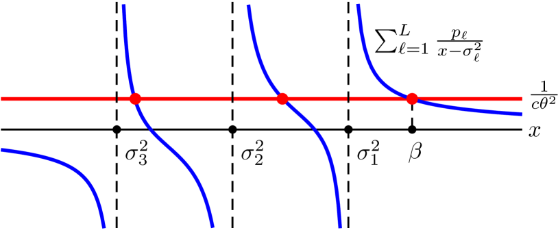
Figure 2: Illustration of the real roots of $B(x)$ for $L=3$ levels. They occur where the sum (blue curve) intersects $1/(c\theta^{2})$ (red line). The largest is $\beta$.

 

To the right of all the noise levels (i.e., for $x$ larger than all the noise levels $\sigma_{\ell}^{2}$), both $A$ and $B$ continuously and monotonically increase from negative infinity to one, and so each has exactly one real root larger than all the noise levels (namely, the largest real root). Thus $\psi\left(b^{+}\right)$ is the largest real root of $A$ and when $\theta>\bar{\theta}$, $\psi\left(\rho\right)$ is the largest real root of $B$.

Using this yields the algebraic form of the prediction:

$$\left|\tilde{u}^{T}\hat{u}\right|^{2}\ \ \underset{{\tiny\begin{array}[]{c}n,d\rightarrow\infty\\ n/d=c\end{array}}}{\overset{a.s.}{\longrightarrow}}\left\{\begin{array}[]{ll}\frac{A\left(\beta\right)}{\beta B^{\prime}\left(\beta\right)}&B\left(\alpha\right)<0\\ 0&\text{otherwise}\end{array}\right.$$

where $\alpha$ and $\beta$ are, respectively, the largest real roots of $A$ and $B$.

IV-H Further simplify the asymptotic prediction

We further simplify the asymptotic prediction by showing that $B\left(\alpha\right)<0$ is equivalent to $A\left(\beta\right)/\left(\beta B^{\prime}\left(\beta\right)\right)>0$.

To do this, observe that both $\alpha$ and $\beta$ are larger than all the noise levels $\sigma_{\ell}^{2}$, and note that $A\left(x\right)$ and $B\left(x\right)$ are both monotonically increasing in this regime. Thus it follows that

$$B\left(\alpha\right)<0\iff\alpha<\beta\iff 0<A\left(\beta\right)$$

because $B\left(\beta\right)=0$ and $A\left(\alpha\right)=0$.

Furthermore $B^{\prime}\left(\beta\right)>0$ (since $B$ is increasing in this regime) and $\beta>0$. Thus

$$A\left(\beta\right)>0\iff\frac{A\left(\beta\right)}{\beta B^{\prime}\left(\beta\right)}>0$$

Using this equivalence finally leads to the main result in (3).

V Qualitative analysis

This section applies the main result (Theorem 1) in several settings to gain some insights into the performance of PCA.

V-A Dependence on balance of noise variances

Here we would like to understand how the balance of the noise variances affects the performance. We consider a case with two noise levels where we sweep the noise variances $\sigma_{1}^{2}$ and $\sigma_{2}^{2}$ while holding fixed the average noise variance

$$\bar{\sigma}^{2}=p_{1}\sigma_{1}^{2}+p_{2}\sigma_{2}^{2}.$$

In particular, consider

$$c =10 p =\left(0.7,0.3\right)$$

$$\theta =1 \bar{\sigma} =1.3$$

where we sweep over $\lambda\in[0,1]$ and set

$$\sigma_{1}^{2} =\frac{\lambda}{p_{1}\lambda+p_{2}(1-\lambda)}\bar{\sigma}^{2}$$

$$\sigma_{2}^{2} =\frac{(1-\lambda)}{p_{1}\lambda+p_{2}(1-\lambda)}\bar{\sigma}^{2}.$$

As intended, this fixes the average noise variance at

$$\frac{1}{n}\sum_{i=1}^{n}\eta_{i}^{2}=p_{1}\sigma_{1}^{2}+p_{2}\sigma_{2}^{2}=\bar{\sigma}^{2}.$$

Sweeping over $\lambda$ adjusts the breakdown of the average noise variance $\bar{\sigma}^{2}$ across the two noise levels. It is not initially obvious whether better performance will occur halfway when $\lambda=1/2$ or at the extremes when $\lambda=0$ or $\lambda=1$. When $\lambda=1/2$ both noise levels are the same and so all the samples have noise variance $\bar{\sigma}^{2}$ and this reduces to the previously considered homoscedastic case analyzed as an example in [12]. When $\lambda=0$ or $\lambda=1$, some of the points have no noise (and so PCA may do better), but the rest have noise larger than $\bar{\sigma}^{2}$ (and so PCA may do worse).

Figure 3(a) shows that the asymptotic prediction has a peak at $\lambda=1/2$; recovery is best when the two noise levels are the same. In other words, having samples with more noise hurts more than having samples with corresponding less noise helps, regardless of which set is larger. This seems to be a general phenomenon; the same has occurred for other choices of parameters we tried.

To further investigate, we use the same parameters $c,p,\theta$ as before but sweep over both $\sigma_{1}^{2}$ and $\sigma_{2}^{2}$ (independently) and produce a heatmap of the asymptotic prediction, shown in Figure 3(b). On this figure, adjusting $\lambda$ corresponds to moving along the line (shown as light blue dashes):

$$\sigma_{2}^{2}=\frac{1}{p_{2}}\bar{\sigma}^{2}-\frac{p_{1}}{p_{2}}\sigma_{1}^{2},$$

which has slope $-p_{1}/p_{2}=-7/3$. Along this line, the prediction does indeed decrease away from the diagonal $\sigma_{1}^{2}=\sigma_{2}^{2}$.

Figure 3(b) illustrates that the prediction seems to depend primarily on the larger of the two noise variances. This is initially surprising but might be understood by considering the root $\beta$ of $B$. Recall that it is the largest value $x$ satisfying

$$\frac{1}{c\theta^{2}}=\sum_{\ell=1}^{L}\frac{p_{\ell}}{x-\sigma_{\ell}^{2}}$$

as illustrated in Figure 4. This figure suggests that the largest root is heavily influenced by the largest noise variance (it is the nearest pole). As a result, changing the other noise variances has much less impact on $\beta$ and on the prediction. The precise relative impact does depend on the proportions, as seen in Figure 3(b), where the shape of the level curves are not symmetric around $\sigma_{1}^{2}=\sigma_{2}^{2}$ (if the performance depended exclusively on the max of $\sigma_{1}^{2}$ and $\sigma_{2}^{2}$, it would necessarily be symmetric). Nevertheless, for any proportion, large noise variances can drown out the influence of small noise variances.

This insight gives a rough explanation of why it may be generally preferable to have equal noise variances ($\lambda=1/2$) for some fixed average noise variance. Imbalance ($\lambda\neq 1/2$) means that one of the noise variances will be larger and cause the performance to decline even though the other noise variance is smaller.

   

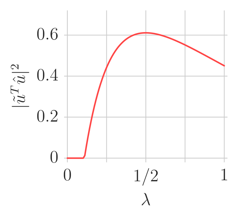
(a) Sweeping over noise levels while keeping the average noise variance fixed at $\bar{\sigma}^{2}=1.69$. When $\lambda=1$, $\sigma_{1}^{2}$ is large and $\sigma_{2}^{2}=0$. When $\lambda=0$, $\sigma_{1}^{2}=0$ and $\sigma_{2}^{2}$ is even larger.

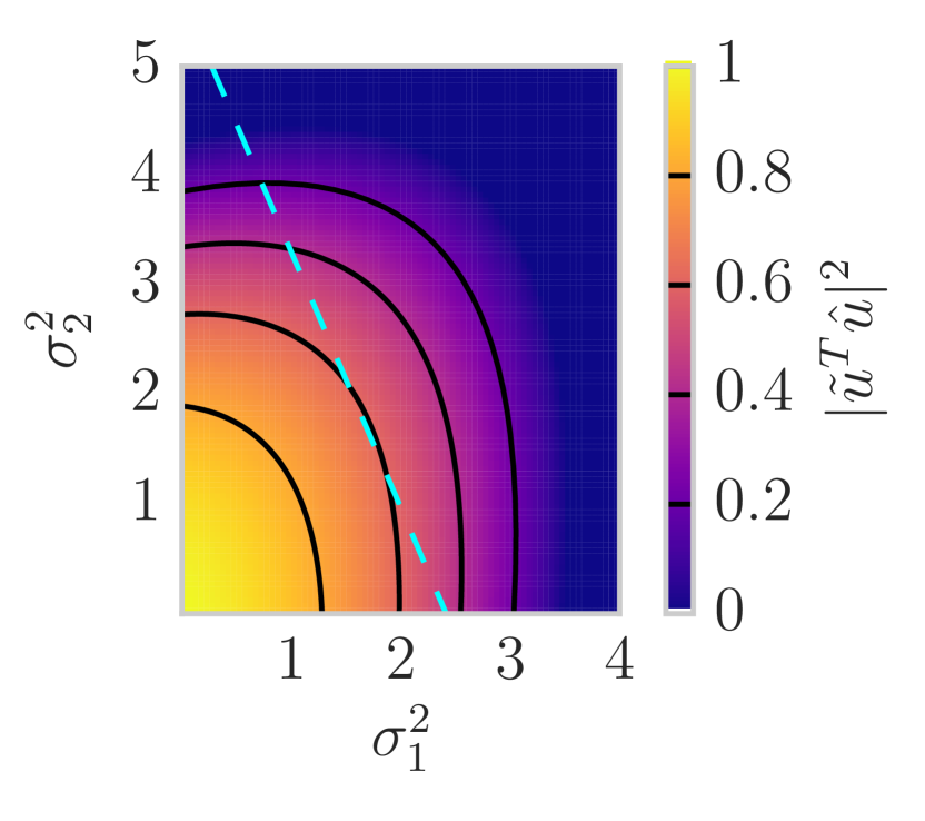
(b) Sweeping over both noise levels independently. The solid black curves are contours. On the dotted cyan line, the average noise variance is $\bar{\sigma}^{2}=1.69$.

Figure 3: Asymptotic prediction under various noise levels for $c=10$, $p=\left(0.7,0.3\right)$, $\theta=1$. Namely, $70\%$ of samples have noise variance $\sigma_{1}^{2}$ and $30\%$ have noise variance $\sigma_{2}^{2}$.

 

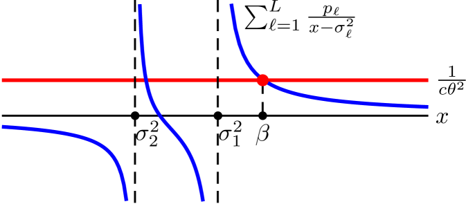
Figure 4: Location of the largest root $\beta$ of $B(x)$ for $\lambda=0.7$ (i.e., $\sigma_{1}^{2}=2.04$ and $\sigma_{2}^{2}=0.874$), $c=10$, $p=(0.7,0.3)$ and $\theta=1$.

 

V-B Dependence on sample-to-dimension ratio and average noise variance

Now consider holding everything constant except for the sample-to-dimension ratio and average noise variance. We first suppose that there is only one noise level (alternatively, two noise levels that are equal). In particular we consider

$$\theta =1 p_{1} =1 \ \sigma_{1}^{2} =\bar{\sigma}^{2}$$

and we sweep over $c>1$ and $\bar{\sigma}^{2}>0$, as shown in Figure 5(a). Note that this is the homoscedastic case analyzed as an example in [12] and Figure 5(a) illustrates the predicted phase transition at $c=\bar{\sigma}^{4}$. In fact, the asymptotic prediction in (3) specializes to the prediction in [12] for the case where there is only one noise level and hence the noise is homoscedastic.

   

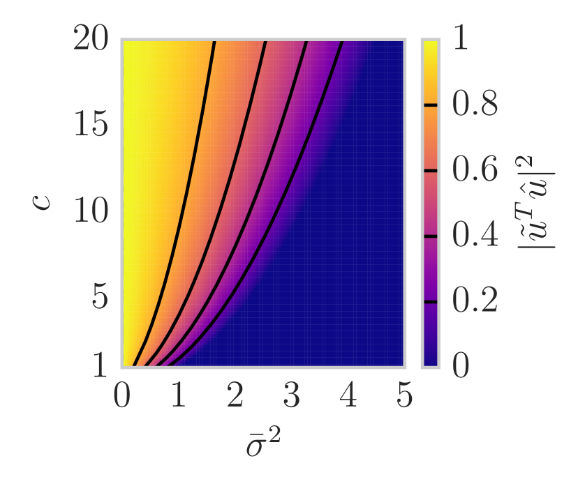
(a) Homoscedastic (i.e., identically distributed) noise.

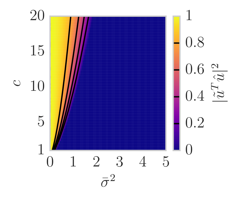
(b) Heteroscedastic (i.e., imbalanced) noise.

Figure 5: Asymptotic prediction as a function of average noise variance $\bar{\sigma}^{2}$ and sample-to-dimension ratio $c$. Contours are overlaid in black. Note that the phase transition in (b) is further left than in (a); more samples are needed to tolerate the same amount of noise.

We now consider an analogous setting where the noise is imbalanced (i.e., heteroscedastic) with

$$p_{1} =0.9 \sigma_{1}^{2}=\frac{1}{2p_{1}}\bar{\sigma}^{2}$$

$$p_{2} =0.1 \sigma_{2}^{2}=\frac{1}{2p_{2}}\bar{\sigma}^{2}$$

so that

$$p_{1}\sigma_{1}^{2}+p_{2}\sigma_{2}^{2}=\frac{1}{2}\bar{\sigma}^{2}+\frac{1}{2}\bar{\sigma}^{2}=\bar{\sigma}^{2}.$$

Figure 5(b) illustrates a similar behavior with a phase transition further left. Namely, more samples are needed than in the homoscedastic setting for the same average noise variance. This agrees with the previous observation that performance for a given average noise variance is best when all the points have the same noise variance (i.e., are homoscedastic).

V-C Dependence on sample proportions

Finally we revisit the sweep carried out in the numerical experiments of Section III. Recall that everything but the proportions were fixed. In particular,

$$c =10 \theta =1 \sigma =(1.8,0.2)$$

and $p_{2}$ varied from $0$ to $1$ with $p_{1}=1-p_{2}$. Figure 1 shows the prediction as a red curve (identical in both sub-figures).

As expected, the performance is best when $p_{2}=1$ and all the samples have the lower noise variance; it is preferable to have a larger proportion of low noise samples. Interestingly, the benefit of having more low noise samples is not uniform through the range. The slope for small $p_{2}$ (close to zero) is less steep than that for high $p_{2}$ (close to one). Hence, having a larger proportion of low noise samples is not as helpful when there are only a few low noise samples otherwise. A careful investigation of this phenomenon would be an interesting area of further study.

VI Discussion and extensions

This paper considered PCA when noise is heteroscedastic and provided a step towards the analysis of the recovery of the subspace. In particular, we provided a simple asymptotic prediction for the recovery of a one-dimensional subspace by PCA from noisy heteroscedastic samples. We provided an example, illustrating how the simple form enables easy and efficient calculation of the asymptotic prediction, as well as an experimental verification of the prediction in simulation. Next, we used the simple form to reason qualitatively about the asymptotic prediction and gain new insights about the performance of PCA. Namely, we found that the performance seems to often be most heavily influenced by the largest noise variance present in the data. Hence, heteroscedasticity tends to have a negative impact on the performance of PCA.

There are many avenues for potential extensions and further work. A natural direction is to extend this work to multi-dimensional subspaces. Another avenue of future work will be to consider a weighted version of PCA, where the samples are first weighted in the objective function (1) to reduce the impact of very noisy points. Unfortunately, applying these weights violates the construction of the subspace coefficients as being identically distributed and so this is a challenging extension. Other avenues include further investigation of the phenomena discussed in the qualitative studies above as well as further study of the algebraic structure of the expressions in the prediction.

References

- [1] J. Wright, A. Ganesh, S. Rao, Y. Peng, and Y. Ma, “Robust principal component analysis: Exact recovery of corrupted low-rank matrices via convex optimization,” in Advances in Neural Information Processing Systems 22, 2009, pp. 2080–2088.
- [2] S. Chatterjee, “Matrix estimation by universal singular value thresholding,” The Annals of Statistics, vol. 43, no. 1, pp. 177–214, 02 2015.
- [3] B. A. Ardekani, J. Kershaw, K. Kashikura, and I. Kanno, “Activation detection in functional MRI using subspace modeling and maximum likelihood estimation,” IEEE Transactions on Medical Imaging, vol. 18, no. 2, pp. 101–114, 1999.
- [4] A. Lakhina, M. Crovella, and C. Diot, “Diagnosing network-wide traffic anomalies,” in Proceedings of the 2004 Conference on Applications, Technologies, Architectures, and Protocols for Computer Communications, ser. SIGCOMM ’04, 2004, pp. 219–230.
- [5] N. Sharma and K. Saroha, “A novel dimensionality reduction method for cancer dataset using PCA and feature ranking,” in Advances in Computing, Communications and Informatics (ICACCI), 2015 International Conference on, 2015, pp. 2261–2264.
- [6] R. Basri and D. W. Jacobs, “Lambertian reflectance and linear subspaces,” IEEE Transactions on Pattern Analysis and Machine Intelligence, vol. 25, no. 2, pp. 218–233, 2003.
- [7] S. Papadimitriou, J. Sun, and C. Faloutsos, “Streaming pattern discovery in multiple time-series,” in Proceedings of the 31st International Conference on Very Large Data Bases, ser. VLDB ’05, 2005, pp. 697–708.
- [8] G. S. Wagner and T. J. Owens, “Signal detection using multi-channel seismic data,” Bulletin of the Seismological Society of America, vol. 86, pp. 221–231, 1996.
- [9] I. Jolliffe, Principal Component Analysis. Springer-Verlag, 1986.
- [10] F. D. la Torre and M. J. Black, “Robust principal component analysis for computer vision,” in Computer Vision, 2001. ICCV 2001. Proceedings. Eighth IEEE International Conference on, vol. 1, 2001, pp. 362–369 vol.1.
- [11] J. He, L. Balzano, and A. Szlam, “Incremental gradient on the grassmannian for online foreground and background separation in subsampled video,” in Computer Vision and Pattern Recognition (CVPR), 2012 IEEE Conference on, 2012, pp. 1568–1575.
- [12] F. Benaych-Georges and R. R. Nadakuditi, “The singular values and vectors of low rank perturbations of large rectangular random matrices,” Journal of Multivariate Analysis, vol. 111, pp. 120 – 135, 2012.
- [13] G. Anderson, A. Guionnet, and O. Zeitouni, An introduction to random matrices. Cambridge university press, 2009, vol. 118.
- [14] G. Pan, “Strong convergence of the empirical distribution of eigenvalues of sample covariance matrices with a perturbation matrix,” Journal of Multivariate Analysis, vol. 101, no. 6, pp. 1330 – 1338, 2010.
- [15] T. Vincent, L. Tenorio, and M. Wakin, “Concentration of measure: fundamentals and tools,” Lecture Notes. [Online]. Available: http://www.stat.rice.edu/ jrojo/PASI/lectures/TyronCMarticle.pdf
- [16] R. R. Nadakuditi and A. Edelman, “The polynomial method for random matrices,” Foundations of Computational Mathematics, vol. 8, no. 6, pp. 649–702, 2008.