Perfectly-matched-layer boundary integral equation method for wave scattering in a layered medium
Abstract
For scattering problems of time-harmonic waves, the boundary integral equation (BIE) methods are highly competitive, since they are formulated on lower-dimension boundaries or interfaces, and can automatically satisfy outgoing radiation conditions. For scattering problems in a layered medium, standard BIE methods based on the Green’s function of the background medium must evaluate the expensive Sommefeld integrals. Alternative BIE methods based on the free-space Green’s function give rise to integral equations on unbounded interfaces which are not easy to truncate, since the wave fields on these interfaces decay very slowly. We develop a BIE method based on the perfectly matched layer (PML) technique. The PMLs are widely used to suppress outgoing waves in numerical methods that directly discretize the physical space. Our PML-based BIE method uses the Green’s function of the PML-transformed free space to define the boundary integral operators. The method is efficient, since the Green’s function of the PML-transformed free space is easy to evaluate and the PMLs are very effective in truncating the unbounded interfaces. Numerical examples are presented to validate our method and demonstrate its accuracy.
1 Introduction
Scattering problems for sound, electromagnetic and elastic waves in layered media are highly relevant for practical applications [10]. Numerical methods that directly discretize the physical domain, such as the finite element method (FEM) [20], are very versatile and widely used, but they become too expensive when the scatterer is large compared with the wavelength. The boundary integral equation (BIE) methods [11] are applicable to structures with piecewise constant material parameters. These methods take care of the outgoing radiation condition automatically and reduce the dimension by one, since the integral equations are formulated on material interfaces or boundaries of obstacles. For many problems, BIE methods can outperform FEM and other domain-discretization methods, and deliver highly accurate solutions with relatively small computing efforts.
For scattering problems in a layered medium, the common BIE methods are based on the Green’s function of the layered background medium [26, 28, 33], so that the intergral equations are formulated on strictly local interfaces or boundaries. However, it is well known that this approach is bottlenecked by the evaluation of Sommefeld integrals arising from the layered-medium Green’s function and its derivatives. Over the past decades, many methods such as high-frequency asymptotics, rational approximations, contour deformations [7, 8, 23, 24, 25], complex images [22, 30, 31], and the steepest descent method [12, 13], have been developed to speed up the computation of Sommefeld integrals. Unfortunately, the computational cost for evaluating the Sommerfeld integrals remains high [6].
An alternative approach is to use the free-space Green’s function, but then the integral equations must also be formulated on the unbounded interfaces separating the different layers of the background medium. Various types of compactly supported functions can be used to truncate the unbounded interfaces and to suppress the artifical reflections from the edges of the truncated sections. Existing methods in this category include the approximate truncation method [18, 27], the taper function method [34, 29, 19], and the windowing function method [4, 21, 5, 14]. In particular, the windowing function method of Bruno et al. [5] can largely eliminate the artificial reflections, since the errors decrease superalgebraically as the window size is increased. Similar good performance can be observed in the hybrid method of Lai et al. [14] that combines windowed layer potentials (in physical space) with a Sommerfeld-type correction (in Fourier space) for scattering problems where the obstacles are close to or even cut through the interfaces of the background layered media.
In this paper, we develop a BIE method based on perfectly matched layers (PMLs) for two-dimensional (2D) scattering problems in layered media. The PML technique is widely used for domain truncations in wave propagation problems [2, 3, 9, 15]. It can be regarded as a complex coordinate stretching that replaces the real independent variables in the original governing equation by complex independent variables, so that the outgoing waves are damped as they propagate into the PML region. Similar to those BIE methods based on the free-space Green’s function, our BIE method avoids evaluating the expensive Sommefeld integrals, but requires integral equations along the interfaces of the background layered medium. But instead of the free-space Green’s function, we use the Green’s function for the PML-transformed free space, so that the truncation of the interfaces follows automatically from the truncation of PMLs. Notice that the Green’s function of the PML-transformed free space can be simply obtained by extending the argument of the usualy Green’s function to complex space following the definition of the complex square root function.
We implement our PML-based BIE method for 2D scattering problems involving two homogeneous media separated by a single interface. The interface is flat except in a finite session which is referred to as the local perturbation. Additional obstacles are also allowed in the homogeneous media. Two common types of incident waves are considered: a plane incident wave and a cylindrical wave due to a point source. The integral equations are established for the scattered wave satisfying Sommefeld radiation condition at infinity. The scattered wave is defined as the difference between the total wave field and a reference wave field obtained from the same indicent wave for the layered background medium (without the local perturbation of the interface and the obstacles).
BIE methods for scattering problem use many different formulations. Some of these formulations are more appropriate for large (i.e. high-frequency) problems, since they give rise to linear systems with better condition numbers, and are thus more efficient when iterative methods are used. Since our purpose is to demonstrate the effectiveness of PML-based BIEs for truncating unbounded interfaces, we adopt a simple formulation that comes from Green’s representation theorem directly. In addition, we calculate the so-called Neumann-to-Dirichlet (NtD) map (mapping Neumann data to Dirichlet data on the boundary) for each subdomain with constant material parameters, so that the final linear system on interfaces or boundaries of the obstacles can be written down in a very simple form.
To approximate the integral equations, we utilize a graded mesh technique [11], a high-order quadrature rule by Alpert [1], and a newly proposed stabilizing technique. Numerical results indicate that our method is highly accurate and the truncation of the unbounded interfaces by PML is very effective. Typically, for a PML with a thickness of one wavelength and discretized with about the same number of points as a typical segment of one wavelength, about seven significant digits can be obtained. Numerical results show that numerical error decays exponentially for (a PML parameter representing the strength of the PML) in whatever range.
The rest of this paper is organized as follows. In sections 2 and 3, we present our PML-based BIE formulation for solving scattering problems in layered media. The numerical schemes for discretizing the integral equations are given in sections 4 and 5. Numerical examples are presented in section 6 to illustrate the performance of our method, and we conclude the paper in section 7.
2 Problem Formulation
In this paper, we mainly focus on two-dimensional TE and TM polarized scattering problems in a planar layered medium with local perturbations and/or obstacles. To clarify our methodology in a simpler setting, we assume that only local perturbations exist in the medium in the following. In general, obstacles make no noticeable difficulties for the scattering problem.
As illustrated in Figure 1,
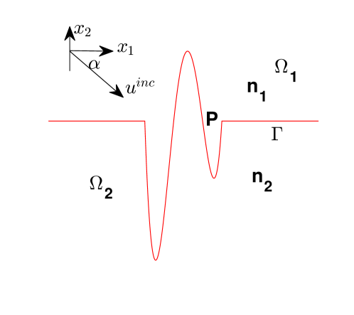
the layered medium is -invariant and consists of two homogeneous layers with constant refractive index for . The interface separating the two layers is flat on but contains a local perturbation curve , smooth or piecewise smooth. Here, denotes the standard Cartesian coordinate system.
The total field , representing the -component of electric field in TE polarization or the -component of magnetic field in TM polarization, solves
| (1) | ||||
| (2) |
where is the freespace wavenumber, is the wavelength, denotes the unit normal vector along pointing toward , denotes the jump of the quantity across , in TE polarization and in TM polarization. Let be an incident wave from the upper medium , and then one usually rewrites
| (3) |
where represents the reflective wave in and represents the transmitted wave in .
In the following, we focus on two common types of incident waves, a plane incident wave and a cylindrical wave due to a source . In the latter case, equation (1) should be replaced by
| (4) |
so that the total field represents a layered-medium Green’s function at the source .
We first discuss the case for plane incident waves. Suppose the incident wave is given by , where denotes the angle between the wave direction and the positive -axis. Neither nor satisfies the Sommerfeld radiation condition since neither of them is outgoing in all directions. To extract an outgoing wave field, we need a reference solution, denoted by , to the scattering problem with perfectly flat interface and with the same incident wave . One easily gets that
| (5) |
where
and . Then,
| (6) |
defines an outgoing wave that satisfies
| (7) | ||||
| (8) |
The transmission condition (2) then becomes
| (9) | ||||
| (10) |
We note that away from the local perturbation curve , and on .
On the other hand, if the incident wave is a cylindrical wave due to a source point . In this case, one easily obtains that, by defining
| (11) |
the difference wave field defines an outgoing wave.
In a typical BIE formulation, the computation of in the whole plane can be reduced to computing and on , governed by the transmission conditions (9) and (10). To solve (9) and (10), we require a relation between and for . In this paper, we make use of Neumann-to-Dirichlet maps that satisfies on the boundary for each outgoing wave . Then, (9) and (10) become
| (12) |
where denotes the identity operator. On solving (12), we immediately obtain that .
In practice, since is unbounded and since decays slowly at infinity, it is impossible to find a finite-dimensional matrix to accurately approximate by directly discretizing the whole boundary of without truncating it. To resolve this issue, we use a PML to enclose the local perturbation curve so that any outgoing wave can be absorbed. Therefore, local transmission condition can be imposed on a finite session of including . In doing so, we first need to construct NtD maps for domains in a PML environment, and this relies on boundary integral equations.
3 Boundary integral equation in a half space
Without loss of generality, we consider the outgoing solution in , that satisfies
| (13) | ||||
| (14) |
for . To simplify the presentation in this section, we assume that the piecewise smooth curve is bounded by a box for . Unless otherwise specified, we will suppress the subscript indexing the domain so that we use , , and to denote , , and , respectively.
3.1 BIE in physical domain
As shown in Figure 2,
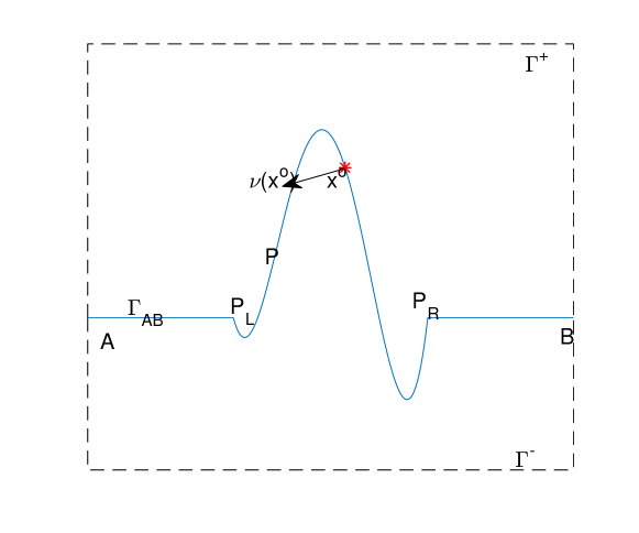
to truncate the unbounded interface , we place a box bounded by to enclose the local perturbation curve so that truncated by the box becomes a bounded curve , which is composed of , , and . Clearly, is truncated into a domain bounded by , where is the dashed line above .
According to [11], one easily obtains the following representation theorem
| (17) |
for . As approaches , one gets the following boundary integral equation (see [11, 16])
| (18) |
for . Here, we have defined the following boundary integral operators
| (19) | ||||
| (20) | ||||
| (21) |
where is the Green’s function of Laplacian equation , and denotes the Cauchy principal integral. Therefore, one obtains the NtD operator that maps to on the bounded curve .
Now, a significant question arises: what boundary conditions should we impose on ? One may directly specify that and on to truncate the NtD operator onto . Unfortunately, the outgoing wave can decay slowly as approaches infinity in . Of course, we may place sufficiently far away from the perturbation curve . However, the computational domain can become extremely large whereas the boundary condition still maintains a low-order accuracy. To address this issue, we propose to introduce a PML to surround the local perturbation , as will be presented below.
3.2 Green’s representation theorem in PML-transformed domain
Specifically, we introduce the complex coordinate stretching function by defining
| (22) |
for , where we take
| (23) |
Domains with nonzero are called the perfectly matched layer. Since is in , the PML does not overlap the local perturbation ; the setup of will be discussed later.
Based on (17), we can analytically continue onto the domain by defining
| (24) |
According to [9], one sees that satisfies
| (25) |
where . Defining the complexified function on , we see that equation (25) can be rewritten by the chain rule as
| (26) |
where , , , and .
As shown in [15], the fundamental solution to (26) is
| (27) |
where the complexified distance function is defined to be
| (28) |
and the half-power operator is chosen to be the branch of with nonnegative real part for ; in other words, satisfies
| (29) |
for .
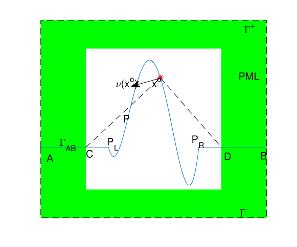
A typical profile of a two-layer medium enclosed by a PML is shown in Figure 3.
We now derive the Green’s representation theorem for in the bounded domain enclosed by the same curve .
For ,
| (30) |
where the last equality follows from the second Green’s identity [17], and we defined the conormal direction and so the conormal derivative .
Similarly, in the limit case when , one obtains the representation formula
| (31) |
for the complexified Laplacian equation
| (32) |
Correspondingly, the related fundamental solution becomes,
| (33) |
3.3 PML-NtD operator
Based on the two representation formulae (3.2) and (31), we are ready to develop the Neumann-to-Dirichlet (NtD) operator on .
Therefore, when approaches an observation point , one easily reproduces for the bounded domain , and satisfies on
| (36) |
where we have defined the following boundary integral operators in a PML environment,
| (37) | ||||
| (38) | ||||
| (39) |
Consequently, we get the PML-NtD operator on , which maps to on .
3.4 Truncating PML-NtD operator onto
Unlike the slowly decaying wave , and decay exponentially at infinity so that it is reasonable to impose and on ; see [2, 3] and section 4.1 below. Therefore, operators and in (36) can be truncated and defined onto curve only, that is, for ,
| (40) |
where the definition of is the same as in (38) but with the integral domain replaced with , etc.
However, the integral cannot be truncated onto since the density function is nonzero on . Nevertheless, it turns out that
| (41) |
where is the interior angle of on even when is in the PML; the proof will be shown in the Appendix. Unfortunately, such a formula cannot be directly used near corners of since numerical discrepancies would appear there [16]. We now discuss how to remove the integral domain for operator .
We distinguish two cases:
-
(1).
Suppose . As shown in Figure 3, for the closed curve
using (41), we see that
(42) where we note that denotes the interior angle. On the other hand, one easily sees that
(43) so that
(44) where the integral in fact becomes a Riemann integral. This implies that
(45) where the subscript indicates that the integral domain is , and the second equality holds since the integral domain is outside the PML. Furthermore, since the integrated domain is outside the PML, one easily gets [16]
(46) We remark that is more stable than ((1).) since is sufficiently far away from and .
-
(2).
Suppose . Since now corresponds to a smooth point of and since it is sufficiently far away from potential corners of , we can directly use the exact formula (41) that
After the truncation, the BIE (40) only depends on the bounded curve . Therefore, by properly discretizing , , and , we are able to approximate the PML-NtD operator on now.
4 Numerical implementation
Suppose the piecewise smooth and open curve is parameterized by , where is the arclength. Since possibly contains corners, to smoothen the non-differentiable , we construct a scaling function following [11], whose derivatives vanish at corners up to order . For example, for a smooth segement of correpsonding to and such that for correspond to two corners, we may take
| (47) |
where
Assume that is uniformly sampled by an even number, denoted by , of grid points with grid size , and that the grid points contain those corner points. The scaling function creates a graded mesh on in the sense that it makes part of grid points cluster around corners while keeping the other part almost uniformly spaced [11].
We shall discuss numerically discretizing the integral operators , , and on in this section. To simplify the notations, we use to denote , and use to denote .
4.1 Setup of the PML
Once reparameterized by parameter , now becomes at least a -class function and we can expect that integrands in (40) are sufficiently smoothened near corners. However, as overlaps with the PML, if in (23) is not properly chosen, those integrands could have weaker regularities at the entrance points and , as shown in Figure 3, since may not be smooth there. We remark here that we do not need to specify since is far away from the horizontal PML regions parallel to .
To ensure that is at least a -class function like at and , we require that derivatives of vanishes at the entrances up to order ; to be on the safe side, we choose . This motivates us to use a function similar to the scaling function in (47) to construct . Suppose the PML on is defined by where denotes the thickness of the PML. Then, for , we take
| (48) |
where
It is not hard to show that bijectively maps to , and satisfies the desired property at . When , one defines .
Now we show how the PML absorbs an outgoing wave. Consider on , a simple outgoing wave for a given as . In the PML, we obtain
| (49) |
where
Clearly, a larger produces a larger so that the imaginary part of becomes larger, and therefore decays more quickly and is absorbed more completely at the boundary of the PML. We will refer to as the absorbing magnitude of the PML in the following.
On the other hand, effectiveness of the PML is also closely related to the magnitude of ; the greater is, the more effective the PML becomes. In general, our unknown outgoing wave restricted on contains many such simple outgoing functions but with different values of . One way to increase the smallest value of among those simple outgoing functions, is to place the PML sufficiently far away from the local perturbation curve . Empirically, for a plane incident wave, the distance between the PML and curve can be around one wavelength; for a cylindrical wave due to a source , it is safer to place the PML at lease one wavelength away from curve as well as the point source .
4.2 Discretizing
According to its definition, acting on at , can be parameterized by
| (50) |
where
| (51) | ||||
| (52) | ||||
| (53) |
Clearly, is not continuous on since is discontinuous at corners. However, since vanishes at corners, the scaled co-normal derivative is smoothened.
One way to discretize the integral in (50) is using the kernel splitting technique developed in [11]. Specifically, the logarithmic singularity of at can be splitted out in terms of
where for , we have
| (54) |
However, such a technique loses high accuracy when the argument of in (54) becomes complex. Specifically, if or is in the PML, may have large imaginary part, giving rise to a blow up function and hence inducing numerical instabilities.
Fortunately, to treat integrands with logarithmic singularities, Alpert [1] developed an efficient quadature rule which does not require a kernel splitting process. Following such an approach, we may discretize the integral in (50) as
| (55) |
where values of , , , and depend on the order of Alpert’s quadrature rule and can be precomputed. For example, in a -th order quadrature formula, we have and ; the associated are given in Table 1.
| 1 | 4.00488 41949 26570 E-03 | 1.67187 96911 47102 E-02 |
|---|---|---|
| 2 | 7.74565 53733 36686 E-02 | 1.63695 83714 47360 E-01 |
| 3 | 3.97284 99935 23248 E-01 | 4.98185 65697 70637 E-01 |
| 4 | 1.07567 33529 15104 E00 | 8.37226 62455 78912 E-01 |
| 5 | 2.00379 69271 11872 E00 | 9.84173 08440 88381 E-01 |
On the other hand, for sufficiently large , it is reasonable to regard as a smooth periodic function so that we may approximate by its trigonometric interpolation [32]
| (56) |
where is the Sinc function, satisfying for and . Utilizing (56), we may rewrite equation (4.2) in terms of for so that we obtain an matrix that satisfies
| (57) |
where the left-hand side represents a column vector produced by evaluating at each element of the column vector for .
4.3 Discretizing
According to its definition, acting on at can be parameterized as
| (58) |
where
| (59) | ||||
| (60) | ||||
| (61) |
Thus, similar to operator , by appling Alpert’s quadrature rule, we discretize the integral in (58) as
| (62) |
By choosing sufficiently large, we may approximate by its trigonometric interpolation like (56) but with replaced by . Consequently, we may rewrite equation (4.3) in terms of for so that we obtain an matrix that satisfies
| (63) |
The discretization of in (46) can be derived similarly.
After the discretization of , , and , one obtains from (40) that
| (64) |
where is a diagonal matrix with entries for ,
Consequently, one gets
| (65) |
where the matrix in fact approximates a scaled PML-NtD operator which maps to on .
4.4 A stabilizing technique
Clearly, to make the approximations of and accurate enough, a high order quadrature rule and a large scaling parameter are always preferable; otherwise, one needs a sufficiently large . Suppose we desire a -th order of accuracy so that nodes and weights of Alpert’s quadrature rule are chosen based on Table 1. To be consistent, we choose in the scaling function . Under such a circumstance, when computing the kernel functions and , we observe that can be as small as . When is close to a corner point, the physical distance can be further shrunk to by the scaling function. Unfortunately, even for a coarse mesh, this can be less than or close to the round-off error in the computation of . In such a situation, is simply regarded as in a double-precision computation. Consequently, division by zero occurs in the computation of and when is close to and when is close to a corner.
To resolve this instability issue, one approach is to reduce the accuracy order to or less. However, this can make the total computational process extremely inefficient in practice. In this section, we develop numerical techiques which can accurately compute and when is close to and is close to a corner.
Observing their expressions (51) and (60), the instability issue comes from the two terms and since they involve subtractions of two extremely close quantities. We discuss first.
Without loss of generality, we assume , so that becomes a piecewise smooth function; note that here may meet some corner. At first, we assume that on is smooth.
To preserve enough significant digits, we require accurately computing
| (66) |
for . There are two approaches to realize this. The first approach is to use the Taylor series of at , that is,
| (67) |
Unfortunately, this approach is ineffective since it is not easy to control the truncation error and since we require the computation of many high order derivatives. The second and more effective approach utilizes the Newton-Lebnitz formula, rewriting (66) in the form,
| (68) |
for . Such an representation gives rise to siginficant advantages. Specifically, the integrand in the primary integral is an quantity so that using numerical integrations (e.g., Gaussian quadrature rules), to compute the integral can highly reduce round-off errors; moreover, we only require the first-order derivative of to obtain accurate result. To ensure stability, the upper limit is also rewritten as an integral form. Consequently, can be evaluated via
| (69) |
We remark that the aim of using arclength but not the grading parameter as the integral variable is to further stabilize the involved computations since integrands roughly become quantities.
Next, we discuss the computation of
| (70) |
Using Newton-Lebnitz formula, we may rewrite as
| (71) |
Using numerical integrations to compute the above double integrals can yield accurate results.
Now, suppose that contains a corner at . Since consists of two smooth segments corresponding to and , respectively, the following splitting
| (72) |
indicates that Newton-Lebnitz formula is applicable for either term on the right-hand side so that numerical integrations can still offer an accurate result for .
As for , we have
| (73) |
where and indicate limits are taken from right side and left side, respectively. Clearly, all the four terms on the right-hand side can be accurately evaluated through numerical integrations.
5 Wave field evaluations
Suppose now in each domain , we have obtained an matrices to approximate the scaled NtD operator , mapping to on , for . Then
| (74) |
where
According to the transmission conditions (9) and (10), the complexified outgoing wave , at the grid points on , satisfies
| (75) | ||||
| (76) |
where we have defined
Thus, by (74), we obtain
| (83) |
which can be solved by
| (84) |
or equivalently,
| (85) | ||||
| (86) |
Consequently, we obtain on .
As for any point , we may directly use (3.2) to compute , that is
| (87) |
where we keep curve only since both and approximately are on . After parameterized by the scaling function in (47), the integrand in (87) becomes periodic and smooth so that by trapezoidal rule, we may approximate
| (88) |
Therefore, in the domain outside the PML, we obtain so that the total wave field .
6 Numerical examples
In this section, we will carry out several numerical experiments to illustrate the proposed methodology. In all examples, the physical region is defined as , while the PML region is defined as with thickness . Therefore, the truncated interface is just restricted on , while the physical region on , denoted by below, is just restricted on . To achieve a high-order accuracy, we take in the scaling function associated with the -th order Alpert’s quadrature rule, using nodes and weights defined in Table 1. We will mainly consider TM-polarization problems.
6.1 Example 1: Perfectly flat surface
To validate our method, the first example is a perfectly flat surface , where , , and the freespace wavelength so that . When represents a plane incident wave, in (5) is the exact solution, making in both and . To avoid such trivial solutions, we here test the case when is a cylindrical wave due to a point source , so that represents a layered Green’s function at .
In the implementation, although is smooth, we still set as an artificial corner since it is close to the source . As shown in [25], an explicit expression of the layered Green’s function is available so that we can obtain the exact solution for reference.
Taking , and , we compute , and compare it with the exact solution on , as shown in Figure 4.
(a)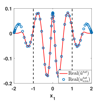 (b)
(b)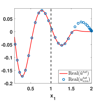
Clearly, on , and coincide very well; in the PML region corresponding to , decay quickly to and still oscillates with a slowly decaying amplitude, as what we are expecting. Figure 5
(a)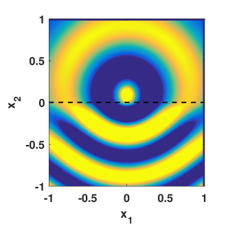 (b)
(b)
show numerical and exact solutions of the real part of in a box , where Figure 5(a) is based on a numerical solution using grid points on . Obviously, they coincide with each other quite well.
To illustrate the order of accuracy, we study numerical error of on against the number of grid points in discretizing when . Since grid points vary for different values of , we choose to evaluate at grid points on when , referred to as a reference set of points, to realize the comparison; for , we just interpolate the numerical solution onto the reference set of points by (56). Using the exact solution as a reference solution, we compute numerical errors for different values of , as depicted in Figure 6(a),
(a)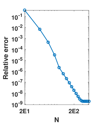 (b)
(b)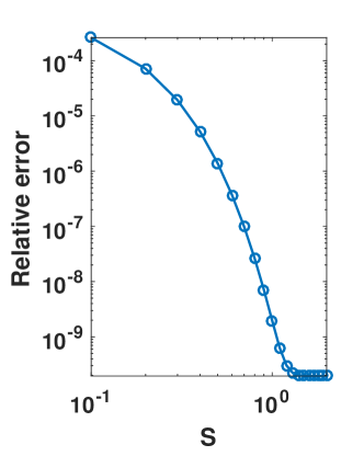
where the vertical axis represents the relative error, the horizontal axis represents , and both axes are logarithmically scaled. Clearly, slope of the decaying part of the curve reveals that our method exhibits at least a seventh-order accuracy.
To illustrate that our PML effectively terminates the outgoing wave, we now fix and compute at grid points on for different values of , ranging from to ; the grid points now are independent of . Using the exact solution as a reference solution, we compute relative errors for different values of , as shown in Figure 6(b), where both axes are logarithmically scaled. We observe that the relative error decays exponentially at the beginning for in a range of small values, and however it terminates for larger . We remark that to maintain an exponentially decaying error for larger , one has to choose larger to increase the number of points in the PML and to decrease the discretization error. From Figure 6, we easily see that the numerical solution for and attains eight significant digits.
To conclude this example, we observe that numerical accuracy in fact can be improved by two approaches: increasing and increasing . When exact solution is not available, it is reasonble that one combines the convergence curve of relative error against for a fixed , and the convergence curve of relative error against for a fixed to truly discover how accurate the solution has obtained, as will be shown below.
6.2 Example 2: Two semicircles
In the second example, we consider a local perturbation that consists of two connected semicircles of radius ; the interface is shown as dotted line in Figure 7. Suppose again , and with wavelength . We consider two incident waves:
-
(i)
a plane incident wave with incident angle ;
-
(ii)
a cylindrical wave due to point source .
In the implementation, we take and so that becomes while the PML region is . The total wave field for the two incident waves in is computed and plotted in Figure 7 (a) and (b), respectively, based on a numerical solution using grid points on .
(a)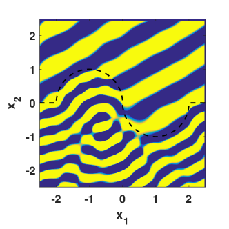 (b)
(b)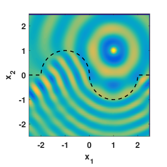
To illustrate the order of accuracy for either incident wave, we compute numerical error of on against the number of grid points when . As in example 1, a reference set of points is chosen as the grid points on when . The reference solution is obtained by computing at the reference set of points when grid points are used. Numerical results for both incident waves are shown in Figure 8,
(a)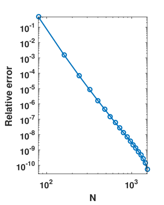 (b)
(b)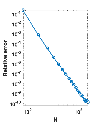
which shows that our results exhibit a seventh-order accuracy for both incident waves.
To illustrate that our PML effectively terminates the outgoing wave for each incident wave, we now fix and compute at grid points on for different values of , ranging from to ; the grid points now are independent of . Considering the numerical solution for as a reference solution, we compute relative errors for different values of . Numerical results are shown in Figure 9.
(a)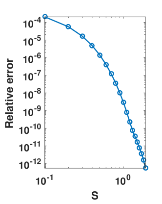 (b)
(b)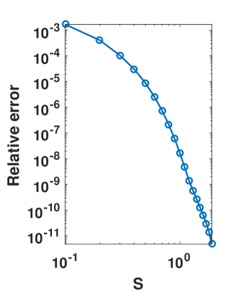
Clearly, we observe that numerical error for each incident wave decays exponentially at the beginning when is not very large, and then decays algebraically for larger as is fixed.
At last, combining Figures 8(a) and 9(a), we see that our numerical solution for the plane incident wave attains eight significant digits when and . Similarly, combining Figures 8(b) and 9(b), we see that our numerical solution for the cylindrical incident wave attains eight significant digits when and .
6.3 Example 3: An obstacle above the interface
In this example, we study a more complicated structure, where an obstacle is placed above the interface. With the obstacle invovled, our PML-based BIE formulation only requires an extra NtD operator defined on the boundary of the obstacle, which can be obtained by a regular BIE in physical domain as described in [16]. Then, according to transmission conditions on the obstacle and the interface, the final linear system can be obtained with ease.
Suppose refractive index of the obstacle is , , , and with . The basic structure is shown in Figure 10, where a drop shape is placed one unit above the interface which contains five uniformly spaced indentations. We consider two incident waves:
-
(i)
a plane incident wave with incident angle ;
-
(ii)
a cylindrical wave due to point source .
In the implementation, we take and so that becomes , while the PML domain becomes . The total wave field for the two incident waves in is computed and plotted in Figure 10 (a) and (b), respectively, based on a numerical solution on and the obstacle boundary , using grid points on ( points per segment) and grid points on , the boundary of the obstacle.
(a)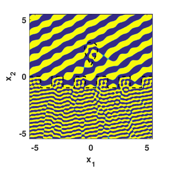 (b)
(b)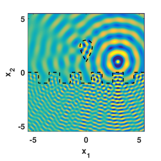
To illustrate the order of accuracy for either incident wave, we study numerical error of on against the number of grid points in discretizing when , where we fix the number of grid points on to be . As in example 1, a reference set of points is chosen as the grid points on when . The reference solution is obtained by computing at the reference set of points when grid points are used. Numerical results for both incident waves are shown in Figure 11,
(a)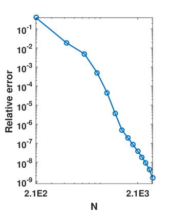 (b)
(b)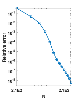
which shows that our results roughly exhibit a seventh-order accuracy for both incident waves.
To illustrate that our PML effectively terminates the outgoing wave for each incident wave, we now fix and compute at grid points on for different values of , ranging from to ; the grid points now are independent of . Considering the numerical solution for as a reference solution, we compute relative errors for different values of . Numerical results are shown in Figure 12.
(a)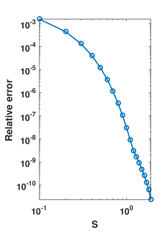 (b)
(b)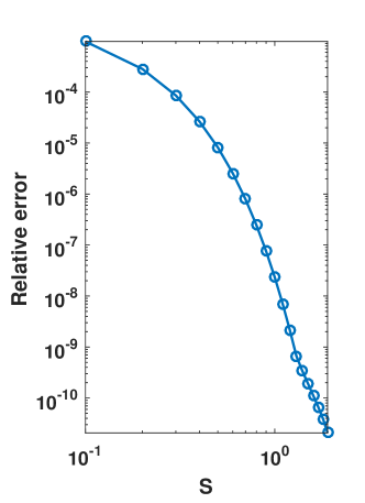
Clearly, we observe that numerical error for each incident wave decays exponentially at the beginning when is not very large, and then decays algebraically for larger as is fixed.
At last, combining Figures 11(a) and 12(a), we see that our numerical solution for the plane incident wave attains seven significant digits when and . Similarly, combining Figures 11(b) and 12(b), we see that our numerical solution for the cylindrical incident wave attains seven significant digits when and .
6.4 Example 4: Interface with different elevations at infinity
In previous examples, flat part of the interface away from the local perturbation have the same elevations at infinity. However, if the flat part has different elevations toward infinity, then all existing methods based on layered Green’s function break down since now for the background layered medium, an explicit form of the layered medium Green’s function in terms of Sommefeld integrals is hard to develop. To conclude this section, we study such a challenging example.
For a plane incident wave, using a flat part on one side (left or right) to define can only suppress the reflective and transmittive waves in on the same side but not on the other side, since the reflection and transmission coefficients are different on each side. Consequently, it is possible that the difference field is not outgoing in all directions, e.g., if a normal incident wave. The current PML-based BIE formulation fails in this case. We expect to address this issue in an ongoing project.
Fortunately, when is a cylindrical wave due to a point source, we may still use defined in (11) to construct an outgoing wave such that our PML-based BIE formulation still works. To justify the methodology, we test a very simple structure where two half-lines with different elevations are connected just by a line segment of unit, as shown in Figure 13, where we suppose , and with wavelength . We consider a cylindrical incident wave due to point source .
In the implementation, we take and so that becomes , while the PML domain becomes . The total wave field for the incident wave in is computed and plotted in Figure 13,
(a)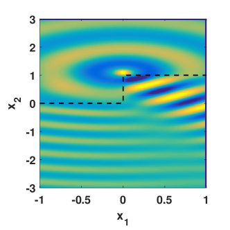
based on a numerical solution using grid points on ( points per smooth segment).
To illustrate the order of accuracy, we study numerical error of on against the number of grid points in discretizing when . As in example 1, a reference set of points is chosen as the grid points on when . The reference solution is obtained by computing at the reference set of points when grid points are used. Numerical results are shown in Figure 14(a),
(a)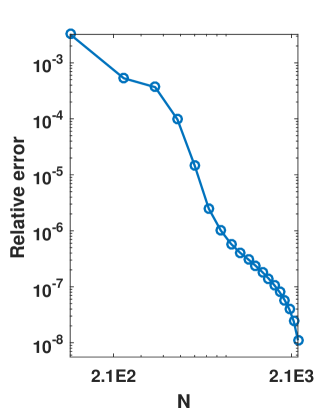 (b)
(b)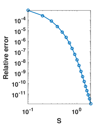
which shows that our results roughly exhibit a fourth-order accuracy.
To illustrate that our PML effectively terminates the outgoing wave, we now fix and compute at grid points on for different values of , ranging from to ; the grid points now are independent of . Considering the numerical solution for as a reference solution, we compute relative errors for different values of . Numerical results are shown in Figure 14 (b). Clearly, we observe that numerical error decays exponentially at the beginning when is not very large, and then decays algebraically for larger as is fixed.
7 Conclusion
For 2D scattering problems in layered media with unbounded interfaces, we developed a PML-based BIE method that relies on the Green’s function of PML-transformed free space. The method avoid the difficulty of evaluating the expensive Sommerfeld integrals in common BIE methods based on Green’s functions of layered media. Similar to other BIE methods based on the free space Green’s function, integral equations are formulated on unbounded interfaces of the background media and these interfaces must be truncated. Although existing methods such as the windowing function method [4, 21, 5, 14], are also effective in truncating interfaces, our method is particularly simple, since the truncation simply follows the well-established PML technique. Notice that the Green’s function of PML-transformed free space is simply obtained from the usual Green’s function by extending the argument to complex space, and it is very easy to evaluate.
Since our main purpose is to develop a PML-based method and demonstarte its effectiveness for truncating the unbounded interfaces, we have used a simple BIE formulation involving the single- and double-layer boundary integral operators only. In addition, we used the DtN maps to simplify the final linear system. Numerical examples are presented for scattering problems involving two homogeneous media separated by an interface with local perturbations, and possibly with additional obstacles. The integral equations are discretized using a graded mesh technique, Alpert’s sixth order hybrid Gauss-trapezoidal rule for logarithmic singularities, and a stabilizing technique. Numerical results indicate that the truncation of interfaces by PML is highly effective, and accurate solutions can be obtained using PMLs with a thickness of one wavelength.
Although our current implementation is somewhat limited, the PML-based BIE method can be extended in a number of directions. Obviously, the method can be used to study scattering problems in multi-layered media with local perturbations, embedded obstacles and penetrable structures. Besides scattering problems, the method can also be used to study eigenvalue problems, such as the problem for guided modes in open waveguide structures. We are planning to address some of these problems in our future works.
Acknowledgement
Y. Y. Lu is partially supported by the Research Grants Council of Hong Kong Special Administrative Region, China (Grant No. CityU 11301914). J. Qian is partially supported by NSF grants 1522249 and 1614566.
Appendix
In this appendix, we will show that equation (41) holds for any on .
At first, using the Green’s representation theorem, we easily see that
| (89) |
where is the boundary of circle of radius centered at , and the unit normal vector now points toward .
Thus for sufficiently small , one can parameterize by for where the inner angle .
Clearly, according to its definition (39), we can discretize as
| (90) |
By definitions of complex stretched coordinates transformation (22), on the boundary , we have
| (91) |
and similarly,
| (92) |
Thus,
| (93) |
Clearly, if is outside the PML so that , then
If is inside the PML so that is just a smooth point away from the perturbation curve , then we easily see that , , and the inner angle . In this case,
| (94) |
References
- [1] B. K. Alpert. Hybrid gauss-trapezoidal quadrature rules. SIAM Journal on Scientific Computing, 20(5):1551–1584, 1999.
- [2] J.-P. Berenger. A perfectly matched layer for the absorption of electromagnetic waves. Journal of Computational Physics, 114(2):185 – 200, 1994.
- [3] J.-P. Berenger. Three-dimensional perfectly matched layer for the absorption of electromagnetic waves. Journal of Computational Physics, 127(2):363 – 379, 1996.
- [4] O. P. Bruno and B. Delourme. Rapidly convergent two-dimensional quasi-periodic Green function throughout the spectrum including wood anomalies. Journal of Computational Physics, 262:262 – 290, 2014.
- [5] O. P. Bruno, M. Lyon, C. Pérez-Arancibia, and C. Turc. Windowed green function method for layered-media scattering. SIAM Journal on Applied Mathematics, 76(5):1871–1898, 2016.
- [6] W. Cai. Algorithmic issues for electromagnetic scattering in layered media: Green’s functions, current basis, and fast solver. Advances in Computational Mathematics, 16(2):157–174, 2002.
- [7] W. Cai. Computational Methods for Electromagnetic Phenomena. Cambridge University Press, New York, NY, 2013.
- [8] W. Cai and T. J. Yu. Fast calculations of dyadic Green’s functions for Electromagnetic scattering in a multiplayered medium. J. Comput. Phys., 5(5):247–251, 2000.
- [9] Z. Chen and X. Xiang. A source transfer domain decomposition method for Helmholtz equations in unbounded domain. SIAM Journal on Numerical Analysis, 51(4):2331–2356, 2013.
- [10] W. C. Chew. Waves and fields in inhomogeneous media. IEEE PRESS, New York, 1995.
- [11] D. Colton and R. Kress. Inverse Acoustic and Electromagnetic Scattering Theory (3rd Edition). Springer, 2013.
- [12] T.J. Cui and W.C. Chew. Efficient evaluation of Sommerfeld integrals for tm wave scattering by buried objects. Journal of Electromagnetic Waves and Applications, 12(5):607–657, 1998.
- [13] T.J. Cui and W.C. Chew. Fast evaluation of Sommerfeld integrals for em scattering and radiation by three-dimensional buried objects. IEEE Transactions on Geoscience and Remote Sensing, 37(2):887–900, Mar 1999.
- [14] J. Lai, L. Greengard, and M. OŃeil. A new hybrid integral representation for frequency domain scattering in layered media. submitted, arXiv:1507.04445v2, 2015.
- [15] Matti Lassas and Erkki Somersalo. Analysis of the PML equations in general convex geometry. Proceedings of the Royal Society of Edinburgh: Section A Mathematics, 131(5):1183–1207, 2001.
- [16] W. Lu and Y. Y. Lu. Efficient high order waveguide mode solvers based on boundary integral equations. Journal of Computational Physics, 272:507 – 525, 2014.
- [17] W. McLean. Strongly Elliptic Systems and Boundary Integral Equations. Cambridge University Press, 2000.
- [18] A. Meier and S. N. Chandler-Wilde. On the stability and convergence of the finite section method for integral equation formulations of rough surface scattering. Mathematical Methods in the Applied Sciences, 24(4):209–232, 2001.
- [19] D. Miret, G. Soriano, and M. Saillard. Rigorous simulations of microwave scattering from finite conductivity two-dimensional sea surfaces at low grazing angles. IEEE Transactions on Geoscience and Remote Sensing, 52(6):3150–3158, June 2014.
- [20] P. Monk. Finite Element Methods for Maxwell’s Equations. Oxford University Press, 2003.
- [21] J. A. Monro. A super-algebraically convergent, windowing-based approach to the evaluation of scattering from periodic rough surfaces. Dissertation (Ph.D.), California Institute of Technology., 2008.
- [22] M. Ochmann. The complex equivalent source method for sound propagation over an impedance plane. The Journal of the Acoustical Society of America, 116(6), 2004.
- [23] V. I. Okhmatovski and A. C. Cangellaris. Evaluation of layered media Green’s functions via rational function fitting. IEEE Microwave and Wireless Components Letters, 14(1):22–24, Jan 2004.
- [24] M. Paulus, P. Gay-Balmaz, and O. J. F. Martin. Accurate and efficient computation of the Green’s tensor for stratified media. Phys. Rev. E, 62:5797–5807, Oct 2000.
- [25] C. Pérez-Arancibia and O. P. Bruno. High-order integral equation methods for problems of scattering by bumps and cavities on half-planes. J. Opt. Soc. Am. A, 31(8):1738–1746, Aug 2014.
- [26] Balth Van Der Pol. Theory of the reflection of the light from a point source by a finitely conducting flat mirror, with an application to radiotelegraphy. Physica, 2(1):843 – 853, 1935.
- [27] M. Saillard and G. Soriano. Rough surface scattering at low-grazing incidence: A dedicated model. Radio Science, 46(5):n/a–n/a, 2011. RS0E13.
- [28] A. Sommerfeld. Über die ausbreitung der wellen in der drahtlosen telegraphie. Annalen der Physik, 333(4):665–736, 1909.
- [29] P. Spiga, G. Soriano, and M. Saillard. Scattering of electromagnetic waves from rough surfaces: A boundary integral method for low-grazing angles. IEEE Transactions on Antennas and Propagation, 56(7):2043–2050, July 2008.
- [30] G. Taraldsen. The complex image method. Wave Motion, 43(1):91 – 97, 2005.
- [31] D. J. Thomson and J. T. Weaver. The complex image approximation for induction in a multilayered earth. Journal of Geophysical Research, 80(1):123–129, 1975.
- [32] L. N. Trefethen. Spectral Methods in MATLAB. SIAM, 2000.
- [33] H. Weyl. Ausbreitung elektromagnetischer wellen über einem ebenen leiter. Annalen der Physik, 365(21):481–500, 1919.
- [34] Z. Zhao, L. Li, J. Smith, and L. Carin. Analysis of scattering from very large three-dimensional rough surfaces using mlfmm and ray-based analyses. IEEE Antennas and Propagation Magazine, 47(3):20–30, June 2005.