How Many Components should be Retained from a Multivariate Time Series PCA?

Abstract

We report on the results of two new approaches to considering how many principal components to retain from an analysis of a multivariate time series. The first is by using a “heat map” based approach. A heat map in this context refers to a series of principal component coefficients created by applying a sliding window to a multivariate time series. Furthermore the heat maps can provide detailed insights into the evolution of the structure of each principal component over time. The second is by examining the change of the angle of the principal component over time within the high-dimensional data space. We provide evidence that both are useful in studying structure and evolution of a multivariate time series.

Keywords:

Principal component analysis, heat map, FTSE 250, meteorological time series

JEL Codes: C18

1 Introduction

Principal Components Analysis (Jolliffe, 1986) (PCA) is a multivariate statistical technique used for dimension reduction and to further an understanding of the underlying groups of variables in the data (i.e. variables which may measure the same or similar underlying effect) by extracting an ordered set of uncorrelated sources of variation in a multivariate system.

Often the objective in running a PCA is to reduce the dimensionality of a data set while minimising the loss of information. For example, if a dataset $\bf{x}$ has $p$ variables we would like to replace the $p$ variables with $m$ principal components (PCs) where, ideally, $m\ll p$. A critical question is then – how small can we make $m$ without an unacceptable loss of information?

Several standard methods exist. None of them are based on a statistical test but instead they are “rules of thumb” for deciding on a suitable cutoff. One of the rules is based on the cumulative percentage explained, i.e. retain the components which capture, say, 70% or 90% of the variation. Similarly, Kaiser’s rule (Kaiser, 1960) is based on the principal of retaining components which have greater than or equal power to explain the data than a single variable. Two other methods, the scree plot (Cattell, 1966) and log scree plot (Farmer, 1971), are based on looking for a change in behaviour in the plot of the variance explained (or its log).

Often, after the number of PCs to retain has been determined, they are examined by a subject matter specialist to determine if the PCs have an identifiable meaning. In the context of multivariate time series analysis a second question arises after having made the selection, that is – do the PCs have the same meaning through out the entire sample period? In this paper we propose a two new methods aimed at simultaneously selecting the number PCs to retain and determining if their meaning has changed over time.

In recent years PCA has been widely applied to the study of financial markets and we have chosen to highlight this method with the first example from this field. Given that financial markets are typically characterised by a high degree of multicollinearity, implying that there are only a few independent sources of information in a market, the uncorrelated nature of the eigenvectors extracted by PCA make it an attractive method to apply.

With regards to financial time series, using the spectral decomposition theorem (Jolliffe, 1986, p13), many authorities have divided the eigenvectors into three distinct groups based on their eigenvalues. For example, Kim and Jeong (2005) decomposed a correlation matrix of 135 stocks which traded on the New York Stock Exchange (NYSE) into three parts:

1. The first principal component (PC1) with the largest eigenvalue which they asserted represented a market wide effect that influences all stocks.

2. A variable number of principal components (PCs) following the market component which represented synchronised fluctuations affecting groups of stocks.

3. The remaining PCs indicated randomness in the price fluctuations.

Therefore the questions are: how many components reflect the market and group components and, further, particularly for the groups of stocks, do the PCs have the same meaning through out the entire sample period?

Our second example looks daily maximum temperatures from 105 meteorlogical stations in Australia from 1 March 1975 to 31 December 2015. The stations were chosen based on the completeness of the records.

Similar to financial markets we expect the first principal component to represent overall weather conditions noting that we expect the maximum daily temperatures to have a strong seasonal component. From there we are interested in how many principal component present meaningful components.

This paper adds to the literature by presenting, in addition to some of the most commonly used methods for selecting the number of components to retain for further analysis, two additional methods, one using heatmaps and the other a change in eigenvector angle, to understand the structure of the data and assist in determining how many components to retain.

The remainder of the paper is structured as follows; Section (2) describes the data used, Section (3) describes our proposed new methods, Section (4) presents our results and Section (5) contains our discussion and conclusions.

2 Data

In this paper we present analysis based on two data sets, one financial and one meteorological.

The London Stock Exchange FTSE 250 Index is a capitalisation-weighted index. It consists of the 101st to the 350th largest listed companies. Our data set covers the stocks in the FTSE 250 index as at 30 July 2015, and prices were sourced for the period 28 July 2000 and 30 July 2015 inclusive, a fifteen year period with 3914 trading days. We downloaded the data from Datastream and converted these data to a return series for each stock. We identified which stocks had a complete history for the fifteen year period, and retained a total of 147 stocks. The remaining stocks were listed after 28 July 2000. No allowance was made for the payment of dividends.

Our second example looks at daily maximum temperatures across the Australian continent. Over time there have been 1877 stations maintained by the Australian Buerau of Meteorology. A complete list of meteorlogical sites was be obtained from the Bureau’s web site and 27 Sept, 2016. The oldest station is the Melbourne Regional Office with records dating from May, 1855. The completeness of their records range from 1% to 100%.

Our data is the daily maximum temperatures from 105 stations in Australia from 1 March 1975 to 31 December 2015. The stations were chosen based on the completeness of the records over the period of investigation. The furthest East is Cape Moreton Lighthouse, Queensland, the furthest West is Carnarvon Airport, Western Australia, while the furtherest North is Darwin Airport, Northern Territory and the furtherest South is Cape Bruny Lighthouse, Tasmania.

3 Methods

In multivariate time series analysis a PCA can be used to generate insights into the key components of the variable set. One of the key considerations in applying such a tool is how many principal components should be retained for further analysis. Below we describe three key steps in using heat maps to analyse how many components should be retained. We also briefly describe the standard methods used for this type of analysis.

3.1 Construction of the Heat Maps

In this paper we use a heat map to profile the change in the principal component coefficients over time. The visual nature of the output allows an examination of the heatmap for consistency and patterns.

The three key steps in constructing the heat map are:

1. Determine an appropriate window size;

2. Calculate the coefficients using a sliding window; and

3. Present the heat map.

Each of these steps is discussed below.

3.1.1 Deciding on an Appropriate Window Size

In this study the window size is the minimum number of days (for the meteorological application) or trading days (for the financial application) for which the Kaiser-Meyer-Olkin (Kaiser, 1970; Kaiser and Rice, 1974) measure of sampling adequacy (KMO) does not fall below 0.5. The KMO value is calculated as

$$\text{KMO}=\frac{\sum\sum_{j\neq k}r_{jk}^{2}}{\sum\sum_{j\neq k}r_{jk}^{2}+\sum\sum_{j\neq k}q_{jk}^{2}}$$

where the $r_{jk}$ are the original off-diagonal correlations and the $q_{jk}$ are the off-diagonal elements of the partial-correlation matrix. Thus the KMO statistic is a measure of how small the partial correlations are, relative to the original correlations, the smaller $\sum\sum_{j\neq k}q_{jk}^{2}$ are, the closer the KMO statistic will be to one.

A KMO value of $0.5$ is the smallest KMO value that is considered acceptable for a PCA. The KMO test was performed using functions in the R package psych (Revelle, 2014).

We have applied the KMO measure to both of our examples.

3.1.2 Calculating the Coefficients

PCA can be applied to either a correlation matrix or a covariance matrix. All PCAs reported in this paper were carried out on correlation matrices. PCAs were carried out using standard functions in R (R Core Team, 2014). For a correlation matrix the total variation is equal to the number of variables in the matrix. Correlation matrices were generated from the return series with the cor function in the stat package in base R.

The individual coefficients of the stocks or stations within each component are subject to two mathematical constraints by the PCA. The first is if $\alpha_{i}$ is the coefficient of the stock or temperature station $i$ then $-1\leq\alpha_{i}\leq 1$ and the second that

$$\sum_{i=1}^{N}\alpha_{i}^{2}=1$$

where $N$ is the number of stocks or stations in the sample.

Correlation matrices were calculated for the first $k$ observations where $k$ was determined by the window size. Then a sliding window approach is used to calculate the coefficients for each set of observations. With stock data this means that the first set of coefficients is based on the first $k$ trading days and the next set is base on the second trading day to $k$ + 1 days and so on until the end of the period of investigation. With our daily maximum temperatures the first $k$ observations are the first $k$ days since 1 March 1975. The resulting matrix has the number of rows equal to the number of stocks or stations and the number of columns is the number of trading days or days less the window size. The matrix contains the coefficients. It is these matrices that are visualised using a heat map.

3.1.3 Displaying the Heat Map

To examine the time evolution of the PCs we made heat maps of the $\alpha_{i}$’s using plotting functions in the graphics package in base R. The order of stocks produced by the PCA matches the order in the input correlation matrix. This is unlikely to be the most useful ordering so the stocks were sorted and their order was fixed within each heatmap. In the heatmaps of the $\alpha_{i}$’s for stocks this was done by sorting on the coefficients at the mid-point of the study period, but this choice of sorting point is completely arbitrary. For the weather stations the ordering was based on the station number.

3.2 Variation of Eigenvector Direction

The loadings of each Principal Component are the coefficients of the eigenvectors in the high dimensional data space and so represent a direction within that space. For example, for PC1, this is the direction of largest variation within the space. Thus as an addition or alternative to the heatmaps, a second method of examining the stability of the component meaning over time is to calculate the change in direction of the eigenvector in each subperiod. If this method is being performed instead of, rather than in addition to, generating a heatmap, one must first decide on the window size and calculate the coefficients as described in Sections (3.1.1) and (3.1.2).

We calculate the angle between the eigenvector in the first subperiod and in each of the subsequent sub-periods as the data window is slid across the data. The angle between two eigenvectors can be found from

$$\theta=\arccos{({\bf a}\cdot{\bf b})}$$ (1)

The scalar product ${\bf a}\cdot{\bf b}$ would normally need to be standardised by dividing by $|{\bf a}||{\bf b}|$ but the eigenvectors returned by the software we used were unit vectors rendering the standardisation unnecessary. This generates a time series of angles between the initial and subsequent eigenvectors which are plotted for visual examination.

3.3 Standard methods

There are several standard methods used to evaluate how many principal components should be retained for further analysis. Practitioners typically use more than one method and the methods often report a wide range of possible number of components to retain.

This section briefly describes four methods; cumulative variance, Kaiser’s rule, scree plots, and log eigenvalue diagrams following Jolliffe (1986) Ch. 6.

The cumulative percentage of total variance is the percentage of variance explained by the first $m$ components. If $l_{k}$ is the variance of the $k^{\text{th}}$ PC then $m$ is chosen to be the smallest $m$ such that

$$t_{m}=100\sum_{k=1}^{m}l_{k}\Bigg{/}\sum_{k=1}^{N}l_{k}$$

is greater than a preselected cut-off $t^{*}$. Typically $t^{*}$ is between 70% and 90%. If the PCA is performed on a correlation matrix this simplifies to

$$t_{m}=\frac{100}{N}\sum_{k=1}^{m}l_{k}.$$

The cutoff is a preset value rather than one determined via a statistical test.

The number of components this approach retains varies with the application but the authors’ experience with financial time series data is that this method typically retains many components.

If the PCA is performed on a correlation matrix, then Kaiser’s rule (Kaiser, 1960) can be applied. Kaisers rule selects all PCs for which $l_{k}>1$. This is based on the fact that each PC for which $l_{k}\leq 1$ explains the same or less variation than a single variable on its own. Variations of Kaiser’s rule do exist for covariance matrices, common ones are to select all PCs for which $l_{k}>\bar{l}$ or sometimes more conservatively $l_{k}>0.7\bar{l}$, where $\bar{l}$ is the mean value of the $l_{k}$.

Cattell (1966) discussed using a scree graph which has the component number of the x-axis and the variance associated with each component on the y-axis, plotted as a line graph. That is, it is a plot of $l_{k}$ against $k$. The practitioner then looks at the graph to determine where the “elbow” in the graph is such that it is “steep” to the left and “shallow” to the right. For some applications this decision may be subjective.

A simple variation on this, discussed by Farmer (1971), is to plot $\log l_{k}$, instead of $l_{k}$. That is the log-eigenvalue diagram which plots the component number of the x-axis and the log of the variance associated with each component on the y-axis, plotted as a line graph. As with the scree plot, the practitioner then looks at the graph to determine where cut off should be, this time looking for the point at which the decay becomes linear.

4 Results

This section presents the results of the heat maps and angle change analysis and the outcome of deciding on the number of components using scree plots, log value diagrams, cumulative percentage, Kaiser’s rule. All PCAs reported in this paper were carried out on correlation matrices.

4.1 Heat Maps

As discussed in Section (3) the three key steps in constructing the heat map are: determine an appropriately sized window using the KMO statistic; calculate the coefficients; and present the heat map.

For the stock market application if the window size was 200 trading days then KMO value could not be estimated for some windows. If the window size was 250 then minimum the KMO value was 0.69. Therefore for this application we used a window size of 250 trading days.

For the maximum temperature application if the window size was eight years (2920 days) then the minimum the KMO value was 0.99. With fewer years of data the KMO statistic could not be estimated for some windows. Therefore for this application we used a window size of 8 years or 2920 days.

The coefficients correlation matrices were calculated from the return series on a rolling window of 250 trading days for the stock application (giving 3664 sets of coefficients, with each set having 147 individual coefficients) and the rolling window of 2920 days for the temperature application (giving 11996 sets of coefficients with 105 individual coefficients).

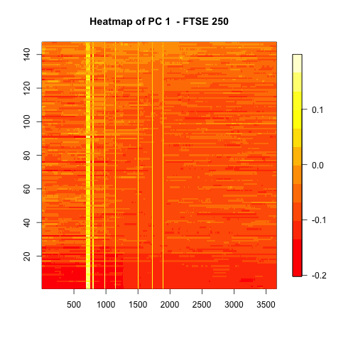
Figure 1: Heatmap of coefficients of PC 1 for the financial application. The horizontal axis is in trading days. The vertical axis is the 147 stocks in the sample sorted by the value of their coefficients in the PCA at the mid-point of the sample.

Figure 2: Angles of eigenvectors of PC 1 between the first and subsequent periods. The points are colour coded black indicates a loading of less than or equal to zero on stock 147 in the heatmap in Figure (1) while green indicates a loading of greater than zero.

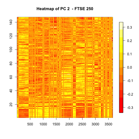
Figure 3: Heatmap of coefficients of PC 2.

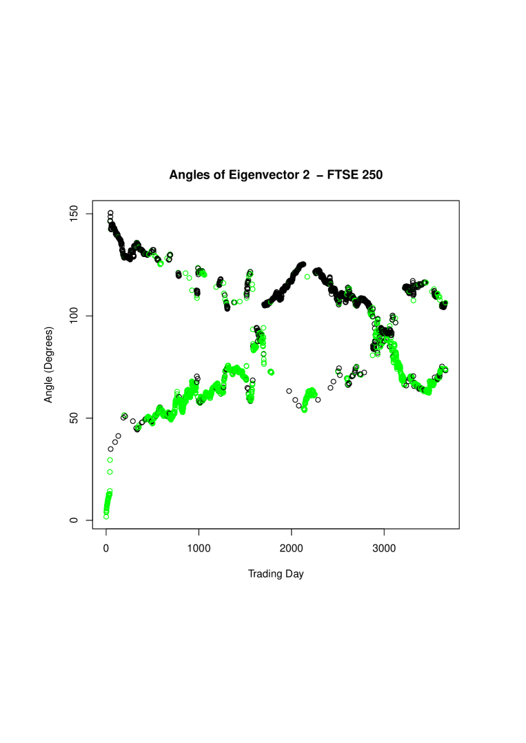
Figure 4: Angles of eigenvectors of PC 2 between the first and subsequent periods. The points are colour coded black indicates a loading of less than or equal to zero on stock 147 in the heatmap in Figure (3) while green indicates a loading of greater than zero.

To examine the time evolution of the principal components we present heat maps of the $\alpha_{i}$’s. Each heat map has time on the x-axis because each set of coefficients was obtained from the PCA applied to the rolling window. The y-axis has the 147 stocks for the stock application or the 105 weather stations for the temperature application. For the stock application these were sorted by the coefficients at the mid-point of the study period for heatmaps of the $\alpha_{i}$’s and for temperature it was sorted by station ID. Note that we call the coefficients structure with lower coefficients at the top “structure A” and the higher coefficients at the top the “structure B”.

The key focus of this subsection is on using heat maps to determine the number of components to retain for further analysis. Below we focus in detail on each of the applications.

For the stock market application clearly the first component (Figure 1) has a structure and offers useful insights into the underlying data. Above we noted that in financial applications the first principal component is considered by other authorities to be the market wide effect. An examination of principal component one showed the majority of the heat map represents structure B as the reds (negative coefficients) are at the bottom. This heat map is consistent with the hypothesis that the first component captures a single market-wide effect.

For the stock market application beyond the first component the heat maps show the coefficients switch between structure A and structure B and this switching happens increasingly rapidly for the higher numbered components. For reasons of space we only present the heat map for PC2 in Figure (3), the remainder are available on request from the authors. The heat map for PC2 is a mixture of structure A with blocks of structure B. The heat map for principal component three had some small sections which are dominated by structure A however some blocks are dominated by rapid change between structure A and structure B. The heat map for principal component four is similar to that of principal component three. The heat map for principal component five is dominated by rapid change with a few other blocks of consistent behaviour, as is component six. The components beyond component six were dominated by rapid change between structure A and B.

Therefore, based on this analysis the maximum number of components to retain for the stock market application would be at most six. However, it would also be reasonable to keep just PC1 noting that only the first component could reasonably be considered to have a nearly constant fundamental structure over the sample period.

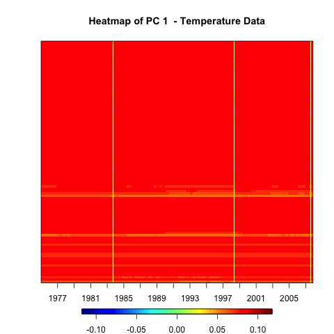
Figure 5: Heatmap of coefficients of PC 1.

Figure 6: Angles of eigenvectors of PC 1.

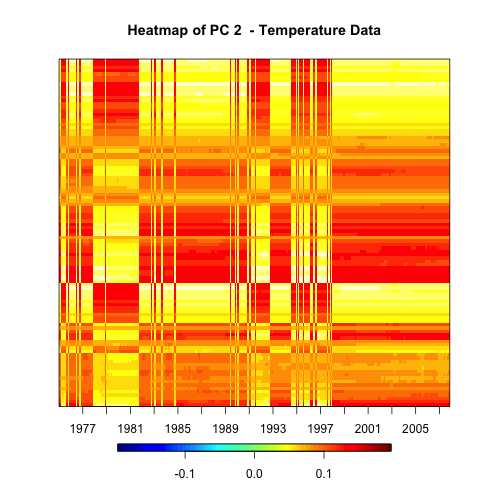
Figure 7: Heatmap of coefficients of PC 2.

Figure 8: Angles eigenvectors of PC 2.

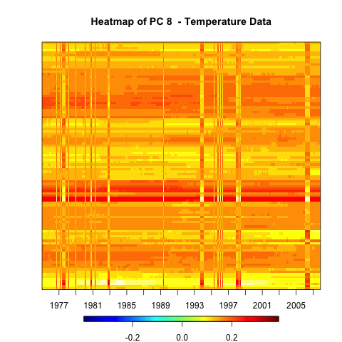
Figure 9: Heatmap of coefficients of PC 2.

Figure 10: Angles eigenvectors of PC 8.

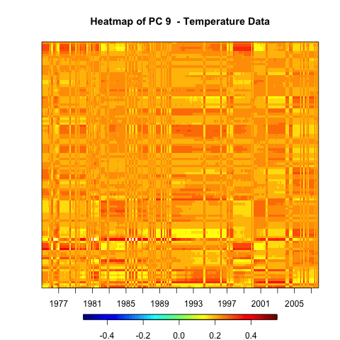
Figure 11: Heatmap of coefficients of PC 9.

Figure 12: Angles eigenvectors of PC 9.

For the temperature application we see a similar behaviour in the first component in that the majority of the heatmap is red. This is likely to represent the similarity in the daily maximum temperature despite the variation across the continent.

For the daily maximum temperature application beyond the first component the heat maps show the coefficients switch between structure A and structure B. The heat map for principal component two is dominated by structure A until the sliding window starting in about 1995 and then is dominated by blocks of structure B. It is worthwhile noting that there is a set of weather stations with the exact opposite pattern to this majority (which are mainly red until 1995 and mainly yellow thereafter).

The heat map for principal component three has a section from the sliding window beginning in 1990 to about 1996 which is different from the majority of the rest of the component. In this section there is rapid change between structure A and structure B.

The heat map for principal component four is dominated by structure B especially from the sliding window beginning in 1989, although the stations with higher numbers do have the lower coefficients.

The heat map for principal component 5 is dominated by structure A with a noticeable section of different behaviour in the sliding windows beginning in 1993 to 2001. Interestingly this component also contains some time invariant behaviour with clear blocks of stations.

The heat map for principal component 6 has some sections of rapid change with a consistent period for the sliding windows beginning in the 1980’s. From here the components begin to have increasingly rapid changes.

4.2 Change in Eigenvector Angle

The details of the selection of the window size and calculation of coefficients for the calculation of the eigenvector angles is identical to that described in Section (4.1) above.

The results for the FTSE 250 index example are presented in Figures (2) and (4). The results for the temperature data are presented in Figures (6), (8), (10) and (12). For reasons of space we have not included the results for PCs three through seven for the temperature data but these are available on request.

For the FTSE 250 data, the angle change for PC1 presents a picture that is consistent with the heat map in Figure (1) in that after an initial change in the angle of the eigenvector in the earliest period in the data it remained stable over the remainder confirming the observation that PC1 is likely to have a single meaning over the whole of the sample period. The angle change for PC2 (Figure 4) presents a picture which supplements the heat map in Figure (3) showing that after the initial rapid change in angle at the beginning of the sample period the angle continues to change over the remainder of the period. The two structures seen in Figure (3) seem to reflect two directions within the data space, but even within that structure the direction was changing over time. Given the change in angle only PC1 can be considered to have retained its meaning over the entire sample period.

For the temperature data, the plots of the angles of the eigenvectors show that the direction of the variation with the data space changes slowly for PCs one through eight. With PC9 there is a substantial change in the behaviour with large changes in angle over time. From this we can consider PCs one through eight to have the same meaning over the sample period.

4.3 Standard methods

We now turn to comparing these results to traditional methods.

We applied cumulative variance with four thresholds present the outcomes for the number of principal components to retain for further analysis in Table 1.

Table 1: Results of applying cumulative variance with four different thresholds

Threshold (%)	Number of components	Number of components
	Stock Market	Daily maximum temperature
60	22	0
70	34	1
80	50	3
90	73	10

Applying Kaisers rule to the stock market application with cutoff of 1 suggested that 38 components be retained for further analysis while with 0.7 it suggested 56. For the maximum daily temperature application the number of components to retain is 8 with a cutoff of 1 and 11 with a cutoff of 0.7.

Figure 13: Scree plots for FTSE 250 data.

Figure 14: Scree plots for temperature data.

The interpretation of the scree plots depends on the practitioner determining where the elbow is in the graph presented in the left panel of Figures (13) and (14). For the stock market application (Figure 13) one could suggest that there are breaks at either five, seven or 10. Retaining more than 10 components would not be reasonable based on the scree plot. For the daily maximum temperatures application (Figure 14) one could suggest that there are breaks at either two, four or six components.

The interpretation of the log value diagrams depends on the practitioner determining where the decay becomes linear in the graphs presented in the right panel of Figures (13) and (14). For the stock market application as with the scree plot, in this example one could suggest that there are breaks at either five, seven or 10. For the daily maximum temperature application the break could be at either one, two, four, six or eight components.

5 Discussion

As noted above, when considering a PCA on time series data it is important to question whether the PCs have the same meaning throughout the entire sample period. Subsequently we have presented two visualisation techniques; one of creating a heat map from a set of eigenvalue coefficients created by applying a sliding window to the time series and a second by checking the change of the angle of the eigenvector with respect to the first. The heat map can then be examined for evidence of structure and the angle for change in direction along which the variation lies within the high-dimensional space.

Our first example data set was from financial time series and comprised of 3914 trading days of the FTSE 250 starting from 28 July 2000. Standard methods of deciding the number of components varied highly from up to 73 for cumulative variance and 109 for Kaisers rule to down to 10 for scree plot and log plot. Our second example data set was from daily maximum temperature series from 105 weather stations in Australia. For this analysis we used data from 1 March 1975 to 31 December 2015. Standard methods of deciding the number of components gave varying results but not more than 10 components (this is primarily because the first component explains more than 60% of the variation). Particularly for the stock market application these rules lead to very diverse recommendations and offer no insights into the behaviour of each component.

Our suggestion is to compliment the standard methods with heat maps and angle variation. The two methods we proposed each have three parts, the first two in common: determine the appropriate window size, then calculate the coefficients using a sliding window. The heat map can be generated from the coefficients. We have found that sorting variables order can improve the interpretability of the heat map. The heat map offers valuable insights into the structure of each principal component and when there is no longer a structure such principal components should not be retained for further analysis.

As indicated in the introduction, a key question when performing a PCA on a multivariate time series is – do the PCs have the same meaning through out the entire sample period? This question is important both for deciding how many components to retain from a PCA and understanding their meaning.

In the context of financial time series analysis this is important because other authorities, such as Kim and Jeong (2005), do assign financial meaning to a number of components. The heat maps presented in Figures (1) and (3) can be usefully applied to answer both questions. These figures show that the first principal component is dominated by structure A (lower coefficients) which is consistent with the hypothesis that the first component is a market-wide component. Components two to six show some evidence of structure, though components beyond PC2 have increasing proportions of time where there is rapid change.

While the results of the scree plot and log eigenvalue plot suggests retaining as many as 10 PCs, the heatmaps indicate that it is not really possible to assign a financial meaning to any PCs beyond PC2. The angle variation analysis suggests only PC1 cold have financial meaning. So while in a statistical sense PCs one through 10 may be retained to explain variation in the data set, a financial subject matter specialist would be unlikely to be able to find useful information beyond one, or at most two, of these PCs.

Our second example applied the same methodology to daily maximum temperatures from 105 weather stations across Asutralia. These heat map for principal component one was dominated by structure A (higher coefficients) and components two through eight some evidence of structure, a conclusion supported by the angle change analysis . These results were consistent with the standard methods, but once again the diagrams offered a greater level of detail.

Thus the heat maps of the PCs offers significantly more insights into the processes that generated the data over time than the other methods commonly used to determine how many PCs to retain from a PCA. Further, the angle change analysis also yielded useful insights.

Appendix A Additional Heatmaps and Angles – FTSE 250

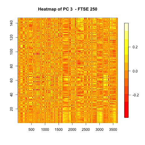
Figure 15: Heatmap of coeffients of PC 3.

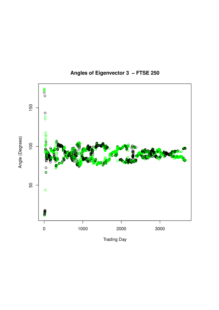
Figure 16: Angles of eigenvectors of PC 3.

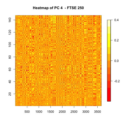
Figure 17: Heatmap of coeffients of PC 4.

Figure 18: Angles of eigenvectors of PC 4.

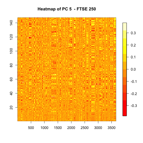
Figure 19: Heatmap of coeffients of PC 5.

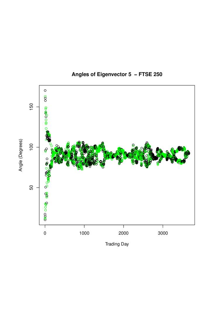
Figure 20: Angles of eigenvectors of PC 5.

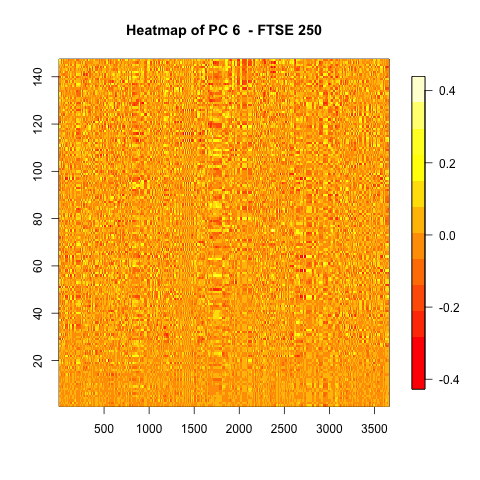
Figure 21: Heatmap of coeffients of PC 6.

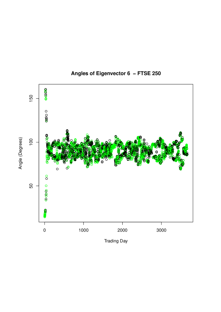
Figure 22: Angles of eigenvectors of PC 6.

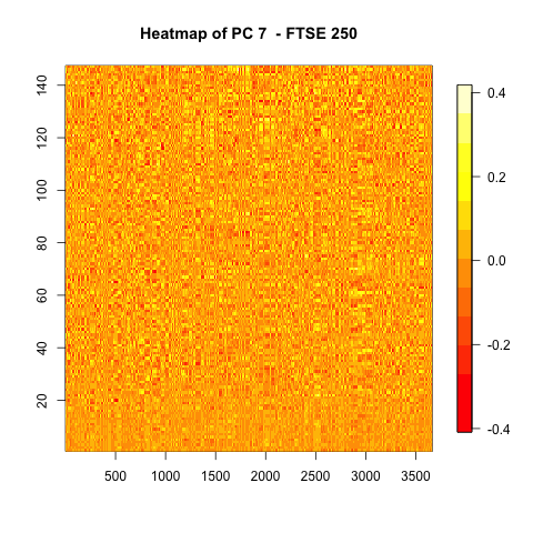
Figure 23: Heatmap of coeffients of PC 7.

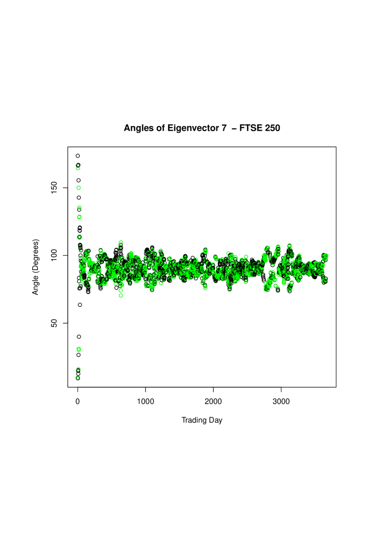
Figure 24: Angles of eigenvectors of PC 7.

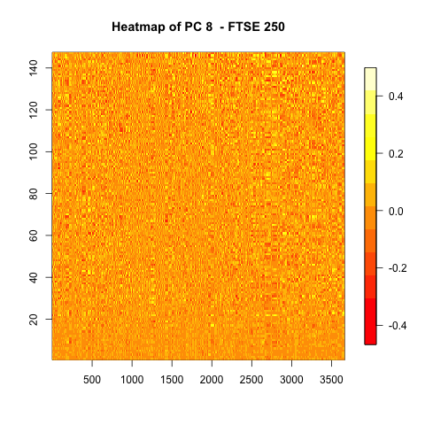
Figure 25: Heatmap of coeffients of PC 8.

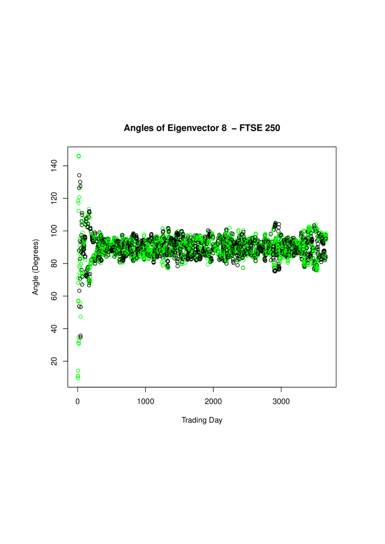
Figure 26: Angles of eigenvectors of PC 8.

Figure 27: Heatmap of coeffients of PC 9.

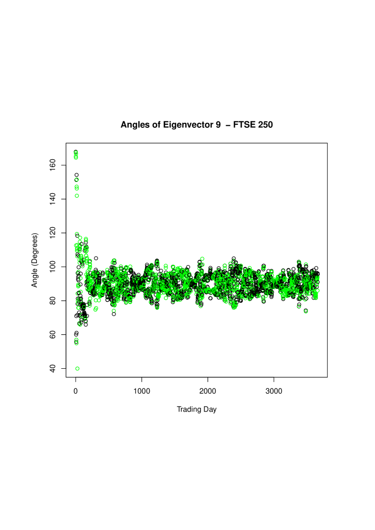
Figure 28: Angles of eigenvectors of PC 9.

Figure 29: Heatmap of coeffients of PC 10.

Figure 30: Angles of eigenvectors of PC 10.

Appendix B Additional Heatmaps and Angles – Meteorology Data

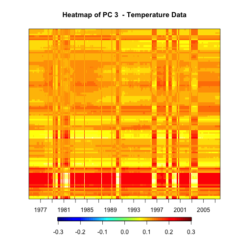
Figure 31: Heatmap of coeffients of PC 3.

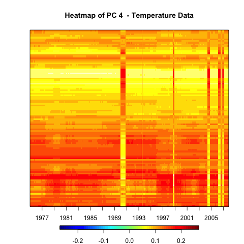
Figure 32: Heatmap of coeffients of PC 4.

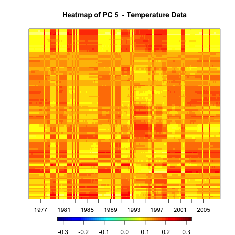
Figure 33: Heatmap of coeffients of PC 5.

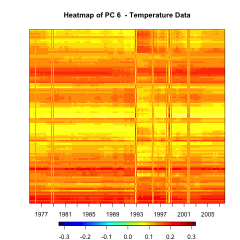
Figure 34: Heatmap of coeffients of PC 6.

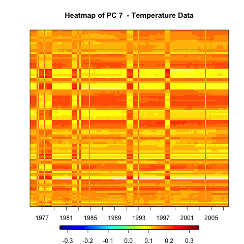
Figure 35: Heatmap of coeffients of PC 7.

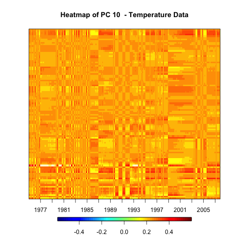
Figure 36: Heatmap of coeffients of PC 10.

References

- Cattell (1966) Cattell, R. B. (1966). The scree test for the number of factors. Multivariate Behavioural Research 1, 245–276.
- Farmer (1971) Farmer, S. A. (1971). An investigation into the results of principal component analysis of data derived from random numbers . Statistician 20, 63–72.
- Jolliffe (1986) Jolliffe, I. T. (1986). Principal Component Analysis. New York: Springer.
- Kaiser (1960) Kaiser, H. F. (1960). The Application of Electronic Computers to Factor Analysis. Educational and Psychological Measurement 20, 141–151.
- Kaiser (1970) Kaiser, H. F. (1970). A second generation little jiffy. Psychometrika 35(4), 401–415.
- Kaiser and Rice (1974) Kaiser, H. F. and J. Rice (1974). Little jiffy. Educational and Psychological Measurement 34(1), 111–117.
- Kim and Jeong (2005) Kim, D.-H. and H. Jeong (2005). Systematic analysis of group identification in stock markets. Physical Review E 72, 046133.
- R Core Team (2014) R Core Team (2014). R: A Language and Environment for Statistical Computing. Vienna, Austria: R Foundation for Statistical Computing.
- Revelle (2014) Revelle, W. (2014). psych: Procedures for Psychological, Psychometric, and Personality Research. Evanston, Illinois: Northwestern University. R package version 1.4.5.