Galaxy-galaxy and galaxy-cluster lensing with the SDSS and FIRST surveys

Abstract

We perform a galaxy-galaxy lensing study by correlating the shapes of $\sim\!\!2.7\times 10^{5}$ galaxies selected from the VLA FIRST radio survey with the positions of $\sim$38.5 million SDSS galaxies, $\sim$132000 BCGs and $\sim$78000 SDSS galaxies that are also detected in the VLA FIRST survey. The measurements are conducted on angular scales $\theta\lesssim 1200$ arcsec. On scales $\theta\lesssim 200$ arcsec we find that the measurements are corrupted by residual systematic effects associated with the instrumental beam of the VLA data. Using simulations we show that we can successfully apply a correction for these effects. Using the three lens samples (the SDSS DR10 sample, the BCG sample and the SDSS-FIRST matched object sample) we measure a tangential shear signal that is inconsistent with zero at the 10$\sigma$, 3.8$\sigma$ and 9$\sigma$ level respectively. Fitting an NFW model to the detected signals we find that the ensemble mass profile of the BCG sample agrees with the values in the literature. However, the mass profiles of the SDSS DR10 and the SDSS-FIRST matched object samples are found to be shallower and steeper than results in the literature respectively. The best-fitting Virial masses for the SDSS DR10, BCG and SDSS-FIRST matched samples, derived using an NFW model and allowing for a varying concentration factor, are ${\rm M}_{200}^{\rm SDSS-DR10}=(1.2\pm 0.4)\times 10^{12}{\rm M}_{\odot}$, ${\rm M}_{200}^{\rm BCG}=(1.4\pm 1.3)\times 10^{13}{\rm M}_{\odot}$ and ${\rm M}_{200}^{\rm SDSS-FIRST}=8.0\pm 4.2\times 10^{13}{\rm M}_{\odot}$ respectively. These results are in good agreement (within $\sim 2\sigma$) with values in the literature. Our findings suggest that for galaxies to be both bright in the radio and in the optical they must be embedded in very dense environment on scales $R\lesssim 1$ Mpc.

1 Introduction

Galaxies can be categorised into two main types; the spiral star forming late type and the elliptical passively evolving early type ones. Furthermore, the spiral galaxies form a sequence defined by their bulge size. Spirals with extremely large bulges are often grouped with elliptical galaxies and are also referred to as early types. Early type galaxies tend to be redder than late type galaxies (Wong et al., 2012; Tojeiro et al., 2013). Observational and theoretical evidence points to the importance of environment conditions on the properties of galaxies. Early type galaxies for example are usually found in less dense areas compared to late type galaxies (e.g. Dressler, 1980). Blanton et al. (2005) found that galaxy colours and luminosities correlate with the galaxy densities. Further, star-formation is strongly associated with the density on small ($\sim$1Mpc) scales (Balogh et al., 2004; Blanton et al., 2006). Finally, measuring dark matter profiles of galaxies can provide us with information related to the galaxies’ merging history (Mandelbaum et al., 2006).

Clusters of galaxies, on the other hand, are among the most promising probes of cosmology and the physics of structure formation. Theoretical predictions (Gunn & Gott, 1972; Press & Schechter, 1974) followed by numerical simulations (Navarro et al., 1997; Evrard et al., 2002) have shown that rich clusters are associated with the most massive collapsed haloes. N-body simulations have predicted that dark matter halos should follow a Universal density profile (Navarro et al., 1996, 1997; Moore et al., 1999; Fukushige & Makino, 2001). The simulations have shown that cluster-size halos should have a relatively shallow and low-concentration mass profile with a density that decreases with increasing radius. Moreover, studies have shown that the evolution of cluster abundance with redshift is a function of a number of cosmological parameters, in particular the normalisztion of the matter power spectrum, $\sigma_{8}$, and the dark energy equation of state, $w$ (White et al., 1993; Viana & Liddle, 1999; Newman & Davis, 2002; Bahcall et al., 2003).

An important parameter that needs to be studied in order to better understand galaxies and galaxy clusters is the tidal gravitational field that they reside in. This gravitational potential is generated from the luminous and dark matter in the vicinity of the galaxy. The visible component of the field may be extracted observationally using galaxy properties such as luminosities or stellar mass. The dark matter on the other hand can not be directly observed, but can be probed indirectly by its gravitational influence on its surroundings. One such probe is the technique of gravitational lensing which provides powerful measurements of the dark matter distribution in the Universe across a wide range of scales (see e.g. Massey et al. 2010 for a review).

Recent years have seen tremendous progress in the detection of weak lensing by galaxies (hereafter galaxy-galaxy lensing) and by galaxy clusters (e.g. Brainerd et al., 1996; McKay et al., 2001; Hoekstra et al., 2003; Sheldon et al., 2004; Heymans et al., 2008; Sheldon et al., 2009; Velander et al., 2014). All of these experiments were conducted in the optical and/or near infra-red (NIR) wavebands. The main reason for this (and in particular for why radio surveys have not traditionally been used) is that at current telescope sensitivity levels, significantly more galaxies are visible in the optical/NIR sky compared to the radio sky. The deep, wide field optical surveys typically used for weak lensing studies routinely deliver $\sim 10$ galaxies arcmin^-2. In contrast, the deepest pencil-beam surveys performed in the radio band to date only reach number densities of $\sim 1-2$ arcmin^-2, and even then, this is typically achieved over only a very small sky area (e.g. Muxlow et al., 2005).

Nevertheless, using radio information in weak lensing studies can in principle be very advantageous, and radio-based analyses are expected to become competitive with the optical when future radio instruments, such as the Square Kilometre Array, come online (Brown et al., 2015; Harrison et al., 2016; Bonaldi et al., 2016). Radio interferometers have a well known and deterministic beam pattern. The instrumental effects can therefore be modelled and removed very accurately. In contrast, in optical weak lensing studies the telescope point spread function (PSF) is known precisely only at discrete locations on the sky, where a point source has been detected, limiting its accurate decomposition.

Additional benefits arise when radio and optical data are combined. Radio surveys are expected to be more sensitive to populations of galaxies that are at higher redshifts compared to what is typically probed in the optical. Combined studies can therefore probe the Universe at earlier times. Additionally galaxy-galaxy lensing depends on the lens-background object configuration, with the signal strength weakened when such pairs are close in redshift. Another advantage of combining optical and radio data for weak lensing studies by galaxies, or by galaxy clusters, lies in the fact that the two surveys trace source populations that are, in general, well separated in redshift. This configuration therefore helps to boost the signal and allows for a clearer identification of the lens and source populations. Moreover as demonstrated in Demetroullas & Brown (2016), an optical-radio combined analysis can be used to suppress position-correlated shape systematics in the data, which, if uncorrected, can generate spurious signals that are orders of magnitude stronger than the sought-after signal. This attribute is particularly relevant for cosmic shear analyses which aim to measure the minute weak lensing signal in background galaxies caused by the intervening large-scale structure of the Universe (c.f. Harrison et al., 2016; Camera et al., 2016).

Finally, combining the data from radio and optical surveys allows one to define novel galaxy lens samples, e.g. jointly in terms of their optical brightness, galaxy morphology, radio luminosity, AGN activity, or gas abundance. We demonstrate this latter feature in this study by defining one of our lens samples to be those galaxies that are bright at both optical and radio wavelengths.

In this study, we use radio data from the Very Large Array (VLA) Faint Images of the Radio Sky at Twenty centimetres (FIRST) survey (Becker et al., 1995) in combination with optical data from the 10th Data Release (DR10) of the Sloan Digital Sky Survey (York et al., 2000; Ahn et al., 2014) to demonstrate the benefits of combining optical and radio surveys for galaxy-galaxy and galaxy-cluster lensing analyses. By cross-correlating the galaxy position and shape information from the optical and radio data respectively, we study the ensemble mass profiles of (i) a sample of optically-selected galaxies, (ii) a sample of galaxy clusters and (iii) a sample of galaxies that have been found to be bright in both wavelengths.

The paper is organised as follows. In Section 2 we present the background weak lensing formalism and in Section 3 we describe the dark matter halo models that we use later to interpret our measurements. In Section 4 we describe the data-sets that were used. Section 5 describes the shape systematics that were identified in FIRST, and that are relevant for this study, and the approach that was adopted to remove them. In Section 6 we describe the simulations that we performed to validate our systematics removal technique and to estimate the uncertainties in our measurements from the real data. In Section 7 we present the results of the analysis of the real data where we measure both galaxy-galaxy and galaxy-cluster lensing signals. We discuss the results and conclude in Section 8.

2 Weak Lensing Background

In the absence of intrinsic galaxy alignments, the weak lensing shear field can be estimated by averaging over galaxy ellipticities:

$$\gamma_{i}=\langle\epsilon_{i}\rangle,$$ (1)

where $\gamma_{1}=\gamma\cos(2\phi)$ and $\gamma_{2}=\gamma\sin(2\phi)$ are the two components of the spin-2 shear field, $\mn@boldsymbol{\gamma}=\gamma_{1}+i\gamma_{2}$, with equivalent expressions for the spin-2 ellipticity field. Here, $\phi$ is the angle that the shear forms relative to an arbitrary reference axis, and the brackets in equation (1) denote an ensemble average.

Expanding $\mn@boldsymbol{\gamma}$ and its complex conjugate in terms of the spin-weighted spherical harmonics, $\,{}_{s}Y_{\ell m}$ (Newman & Penrose, 1966) as

$$\mn@boldsymbol{\gamma}(\Omega) = \gamma_{1}(\Omega)+i\gamma_{2}(\Omega)$$ (2)

$$= \sum_{\ell m}(\kappa_{\ell m}+i\beta_{\ell m})\,_{2}\!Y_{\ell m}(\Omega),$$

$$\mn@boldsymbol{\gamma}^{*}(\Omega) = \gamma_{1}(\Omega)-i\gamma_{2}(\Omega)$$ (3)

$$= \sum_{\ell m}(\kappa_{\ell m}-i\beta_{\ell m})\,_{-2}\!Y_{\ell m}(\Omega),$$

where $s$ denotes the spin and the summation in $m$ is over $-\ell\leq m\leq\ell$, one identifies the so-called $E$- and $B$-mode components of the shear field with the lensing convergence field (denoted $\kappa$) and the odd-parity divergence field (denoted $\beta$). We note that the $\beta$ field is expected to be zero in standard cosmological models and is therefore often used as a tracer of systematic effects. The power spectrum of the convergence field,

$$C_{\ell}^{\kappa\kappa}=\frac{1}{2\ell+1}\sum_{m}\kappa_{\ell m}\,\kappa^{*}_{\ell m},\\$$ (4)

can be related to the 3-D matter power spectrum $P_{\delta}(k,r)$ through (e.g. Bartelmann & Schneider 2001)

$$C_{\ell}^{\kappa\kappa}=\frac{9}{4}\left(\frac{H_{0}}{c}\right)^{4}\Omega^{2}_{m}\int^{r_{H}}_{0}dr\,P_{\delta}\left(\frac{\ell}{r},r\right)\left(\frac{\overline{W}(r)}{a(r)}\right)^{2},$$ (5)

where $H_{0}$ is the Hubble constant, $a$ is the scale factor of the Universe, $r$ is comoving distance, $r_{H}$ is the comoving distance to the horizon and $\Omega_{m}$ is the matter density. The weighting, $\overline{W}(r)$, is given in terms of the normalised comoving distance (or redshift) distribution of the source galaxies, $G(r)dr=p(z)dz$:

$$\overline{W}(r)\equiv\int^{r_{H}}_{r}dr^{\prime}\,G(r^{\prime})\frac{r^{\prime}-r}{r^{\prime}}.$$ (6)

In a similar fashion, one can expand the galaxy over-density field $G$, at an angular position $\bm{\Omega}$, in terms of the (spin-0) spherical harmonics $Y_{\ell m}$ as

$$G(\bm{\Omega})=\sum_{\ell m}G_{\ell m}Y_{\ell m}(\bm{\Omega}).$$ (7)

The power spectrum of such an overdensity map ($C_{\ell}=1/(2\ell+1)\sum_{m}G_{\ell m}G^{*}_{\ell m}$) can be related to the matter power spectrum as

$$C_{\ell}^{GG}=\int^{r_{H}}_{0}\mathrm{d}rP_{\delta}\left(\frac{\ell}{r},r\right)\frac{G(r)}{r}b^{2}_{g}\left(\frac{\ell}{r},r\right)~{},$$ (8)

where $G(r)$ is the normalized comoving distance distribution of the galaxies in the over-density map and $b_{g}(k,r)$ is a scale- and redshift-dependent bias describing the deviation of the galaxy clustering from the dark matter clustering.

By correlating the values in an over-density map with the $\kappa$ and $\beta$ fields of an overlapping shear map, one can construct the two cross-power spectra,

$$C_{\ell}^{G\kappa}=\frac{1}{2\ell+1}\sum_{m}G_{\ell m}\kappa^{*}_{\ell m}~{},$$ (9)

$$C_{\ell}^{G\beta}=\frac{1}{2\ell+1}\sum_{m}G_{\ell m}\beta^{*}_{\ell m}~{}.$$ (10)

As mentioned above, the shear divergence field, $\beta$ is expected to be zero and so we expect $C_{\ell}^{G\beta}=0$. The galaxy over-density convergence cross-spectrum can be related to the 3-D matter power spectrum through (e.g. Joachimi & Bridle, 2010)

$$C_{\ell}^{G\kappa}=\frac{3}{2}\left(\frac{H_{0}}{\mathrm{c}}\right)^{2}\Omega_{\mathrm{m}}\int^{r_{H}}_{0}\mathrm{d}rP_{\delta}\left(\frac{\ell}{r},r\right)\left(\frac{\overline{W}(r)G(r)}{a(r)r}\right)b_{g}\left(\frac{\ell}{r},r\right)r_{g}\left(\frac{\ell}{r},r\right)~{},$$ (11)

where once again $G(r)$ is the normalized comoving distance distribution of the galaxies in the over-density map and $\overline{W}(r)$ is the lensing weighting function appropriate for the sources in the shear map (equation 6). $r_{g}(k,r)$ is a scale- and redshift-dependent cross-correlation coefficient describing the stochasticity of the relationship between the dark matter and galaxy clustering.

2.1 Galaxy-galaxy lensing

The shear components of equation (1) are defined with respect to an arbitrarily defined reference axis. However, in the case where one is interested in the weak lensing distortion in a population of background sources due to the presence of a known foreground object (or “lens”), it is more natural to consider the tangential and rotated shear (or ellipticity), defined by

$$\gamma_{t} = \gamma_{1}\cos(2\omega)+\gamma_{2}\sin(2\omega),$$ (12)

$$\gamma_{r} = -\gamma_{1}\sin(2\omega)+\gamma_{2}\cos(2\omega),$$ (13)

where $\omega$ is the position angle formed by moving counter clockwise from the reference axis to the great circle connecting each source-lens pair. The tangential shear, $\gamma_{t}$, describes distortions in a tangential and/or radial direction with respect to the lens position. The rotated shear, $\gamma_{r}$, describes distortions in the orthogonal direction, at an angle $\pm\pi/4$ to the vector pointing to the lens position.

The galaxy over-density convergence angular cross power spectrum (equation 11) can be related to the tangential shear $\gamma_{t}(\theta)$ (where $\theta$ is the angular separation between lens and source) through (e.g. Hu & Jain, 2004)

$$\gamma_{t}(\theta)=\frac{1}{2\pi}\int\mathrm{d}\ell\,\ell C_{\ell}^{G\kappa}J_{2}({\ell\theta})~{},$$ (14)

where $J_{2}(x)$ is a Bessel function. Since, in the absence of systematics, one expects $C_{l}^{G\beta}=0$, one therefore also expects that the “rotated shear”

$$\gamma_{r}(\theta)=\frac{1}{2\pi}\int\mathrm{d}\ell\,\ell C_{\ell}^{G\beta}J_{2}({\ell\theta})~{},$$ (15)

should be consistent with zero and hence can be used to trace systematics in the data.

In this study we estimate $\gamma_{t}(\theta)$ and $\gamma_{r}(\theta)$ by stacking the measured shapes of VLA FIRST galaxies around the positions of samples of lens galaxies selected from the SDSS catalogue (see Section 4). To estimate the tangential and rotated shear from the data we use the simple estimators:

$$\widehat{\gamma_{t}}(\theta) = \frac{1}{N}\sum_{ls}\epsilon_{t}^{(ls)}(\theta),$$ (16)

$$\widehat{\gamma_{r}}(\theta) = \frac{1}{N}\sum_{ls}\epsilon_{r}^{(ls)}(\theta),$$ (17)

where the tangential and rotated ellipticity ($\epsilon_{t}$ and $\epsilon_{r}$) are defined analogously to the shear quantities (equations 12 & 13) and the summation is over all lens-source ($ls$) pairs (total number $N$) separated by an angle $\theta$. In practice, we further average the $\widehat{\gamma_{t}}(\theta)$ and $\widehat{\gamma_{r}}(\theta)$ estimates within linear bins in angular separation.

3 Dark Matter Halo Models

The theoretical description presented in Section 2 is an accurate model for the linear, and mildly non-linear, evolution of the density perturbations in the Universe. However, on galaxy and galaxy cluster scales the evolution of matter perturbations becomes highly non-linear and the above description breaks down. On these scales, and under the assumption that the lenses have a surface mass density that is independent of the position angle with respect to the lens centre, their density profiles can be predicted using axially symmetric density profile models.

3.1 SIS Model

One of the most widely used axially symmetric dark matter halo models is the singular isothermal sphere (hereafter SIS). The model can be derived assuming that the matter content is an ideal gas in equilibrium confined in a spherically symmetric gravitational potential.

For an isothermal equation of state the gravitational potential ($\Phi$) is given by

$$\Phi=-\sigma_{u}^{2}\ln\left(\frac{\rho}{\rho_{o}}\right)=-\sigma_{u}^{2}\ln\left(\rho^{\prime}\right),$$ (18)

where $\sigma_{u}$ is the velocity dispersion of the gas, $\rho$ is the density of the source, $\rho_{o}$ is the mean density of the Universe and $\rho^{\prime}$ is the fractional density given by $\rho^{\prime}=\rho/\rho_{o}$.

For a given velocity dispersion $\sigma_{u}$, by applying the Virial theorem one can calculate the radius $R_{200}$ and mass $M_{200}$ of the dark matter halo at which its density is equal to 200 times the critical density of the Universe, $\rho_{c}=3H^{2}/8\pi G$ (where $H$ is the Hubble parameter and $G$ is Newton’s gravitational constant).

Rearranging equation (18) with respect to the matter density $\rho^{\prime}$ we get

$$\rho^{\prime}=\exp\left({\frac{-\Phi}{\sigma_{u}^{2}}}\right).$$ (19)

Inserting this in the Poisson equation $\nabla^{2}\Phi=-4\pi G\rho$ we find

$$-\sigma_{u}^{2}\frac{1}{r^{2}}\frac{\mathrm{d}}{\mathrm{d}r}r^{2}\frac{\mathrm{d}}{\mathrm{d}r}\left(\ln\rho^{\prime}\right)=4\pi G\rho^{\prime},$$ (20)

where $r$ is the radial component of the spherical coordinate system. Integrating equation (20) we find

$$\rho^{\prime}(r)=\frac{\rho}{\rho_{o}}=\frac{\sigma_{u}^{2}}{2\pi Gr^{2}}.$$ (21)

Using equation (21), and by projecting the three-dimensional density along the line of sight we obtain the corresponding surface mass density, $\Sigma$:

$$\Sigma(b)=2\frac{\sigma_{u}^{2}}{2\pi G}\int_{0}^{\infty}\frac{\mathrm{d}z}{b^{2}+z^{2}}=\frac{\sigma_{u}^{2}}{2Gb},$$ (22)

where $b$ is the transverse impact parameter (perpendicular to the line of sight) and $z$ is the direction along the line of sight. The model has two pathological properties: it predicts a total source mass that is infinite and a surface mass density that goes to infinity as we move close to the centre of the object ($b=0$). Nevertheless it has been used in many studies as it has been shown to be a good fit to data for angular scales $\theta<3$ arcmin (van Uitert et al., 2011).

The corresponding dimensionless surface mass density is

$$\kappa(\bm{\theta})=\frac{\theta_{E}}{2\bm{\theta}},$$ (23)

where $\bm{\theta}$ is the projected 2-D angular position, and where the Einstein radius $\theta_{E}$ is equal to

$$\theta_{E}=4\pi\left(\frac{\sigma_{u}}{c}\right)^{2}\frac{D_{LS}}{D_{S}}.$$ (24)

Here $D_{LS}$ and $D_{S}$ are the lens-source distance and the distance to the source respectively. In the SIS model the shear $\bm{\gamma}$ relates to the Einstein radius as

$$\mn@boldsymbol{\gamma}(\bm{\theta})=-\frac{\theta_{E}}{2|\bm{\theta}|}e^{2i\alpha},$$ (25)

where $\alpha$ is the polar angle of the galaxy position relative to the lens centre. Equation (25) shows that for an axially-symmetric mass distribution, the shear is always tangentially aligned relative to the mass centre. Expressing $\bm{\gamma}$ in terms of its tangential ($E$-mode) and rotated ($B$-mode) components, for this circularly symmetric lens model, we find (setting $\theta\equiv|\bm{\theta}|$)

$$\gamma_{t}(\theta)=\frac{\theta_{E}}{2\theta}~{}~{}~{}~{}~{}\mathrm{and}~{}~{}~{}~{}~{}~{}\gamma_{r}(\theta)=0.$$ (26)

That is, the shear field should only include a tangential $E$-mode component and, as noted already, the rotated $B$-mode component can be used to test for systematics in the data.

3.2 NFW Model

Navarro et al. (1996) (hereafter NFW) found, using simulations in the framework of CDM cosmology, that the density profile of dark matter halos for objects with masses in the range $10^{12}\lesssim M/h^{-1}\mathrm{M}_{\odot}\lesssim 10^{15}$ can be accurately represented by the radial function

$$\rho(r)=\frac{\rho_{c}\delta_{c}}{(r/r_{s})(1+r/r_{s})^{2}},$$ (27)

where the “scale radius” $r_{s}=r_{200}/c$ is the characteristic radius of the object. $r_{200}$ is the radius of the object where its density is equal to 200 times the critical density of the Universe $\rho_{c}$, $c$ is a dimensionless number known as the concentration parameter and

$$\delta_{c}=\frac{200}{3}\frac{c^{3}}{\ln(1+c)-c/(1+c)}.$$ (28)

The mass of a NFW halo contained within a radius $r_{200}$ is therefore

$$M_{200}\equiv M(r_{200})=\frac{800\pi}{3}\rho_{c}r^{3}_{200}=\frac{800\pi}{3}\frac{\bar{\rho}(z)}{\Omega(z)}r^{3}_{200}~{},$$ (29)

where $\bar{\rho}(z)$ and $\Omega(z)$ are the mean density and the density parameter of the Universe at redshift $z$.

Several algorithms have been developed to estimate the concentration of dark matter halos. All are based on the assumption that the density of the halos reflects the mean cosmic density at the time the halo had formed. This is justified with simulations of structure formation which showed that halos were more concentrated the earlier they were formed. As expected, all models predict that the concentration factor depends on cosmology. Additionally, all models predict that the concentration increases towards lower masses, a direct result of less massive systems collapsing at higher redshifts. For more details on the various algorithms for calculating the concentration factors see Meneghetti (1997) and references therein.

The logarithmic slope of the NFW density profile changes from $-1$ at the centre of the object to $-3$ at large radii. The model therefore predicts a mass density that is flatter than the SIS for the inner part of the halo and steeper in the outskirts. Additionally, in contrast to the SIS, the NFW model has no points where the mass density $\rho$ becomes infinite, making it more realistic.

The NFW surface mass density is obtained by integrating the NFW mass density profile (equation 27) along the line of sight (Wright & Brainerd, 2000). Since the NFW is a spherically symmetric profile, the radial dependence of the shear can be written as

$$\gamma_{t}^{\mathrm{NFW}}(x)=\frac{{\overline{\Sigma}^{\mathrm{NFW}}(x)}-\Sigma^{\mathrm{NFW}}(x)}{\Sigma_{c}}~{},$$ (30)

where we adopt the dimensionless radial distance $x=r/r_{s}$ and the mean surface mass density ${\overline{\Sigma}^{\mathrm{NFW}}(x)}$ is equal to

$${\overline{\Sigma}^{\mathrm{NFW}}(x)}=\frac{2}{x^{2}}\int^{x}_{0}x^{\prime}\Sigma^{\mathrm{NFW}}(x^{\prime}){\mathrm{d}}x^{\prime}.$$ (31)

The radial dependence of the shear is therefore (Wright & Brainerd, 2000)

$$\gamma_{t}^{\mathrm{NFW}}(x)=\left\{\begin{array}[]{l l}\frac{r_{s}\delta_{c}\rho_{c}}{\Sigma_{c}}g_{<}(x),&x<1\\ \frac{r_{s}\delta_{c}\rho_{c}}{\Sigma_{c}}\left[\frac{10}{3}+4\ln\left(\frac{1}{2}\right)\right]~{},&x=1\\ \frac{r_{s}\delta_{c}\rho_{c}}{\Sigma_{c}}g_{>}(x),&x>1~{},\end{array}\right.$$ (32)

where the functions $g_{<}(x)$ and $g_{>}(x)$ are given by

$$g_{<}(x) = \frac{8\,\mathrm{arctanh}\sqrt{(1-x)/(1+x)}}{x^{2}\sqrt{x^{2}-1}}+\frac{4}{x^{2}}{\mathrm{\ln}}\left(\frac{x}{2}\right)-\frac{2}{(x^{2}-1)}$$ (33)

$$+ \frac{4\,\mathrm{arctanh}\sqrt{(1-x)/(1+x)}}{(x^{2}-1)\sqrt{1-x^{2}}}~{},$$

$$g_{>}(x) = \frac{8\,\mathrm{arctan}\sqrt{(x-1)/(1+x)}}{x^{2}\sqrt{1-x^{2}}}+\frac{4}{x^{2}}{\mathrm{\ln}}\left(\frac{x}{2}\right)-\frac{2}{(x^{2}-1)}$$ (34)

$$+ \frac{4\,\mathrm{arctan}\sqrt{(x-1)/(1+x)}}{(x^{2}-1)^{3/2}}~{}.$$

In this study, in addition to directly fitting for the concentration factor $c$ using our measurements from FIRST and SDSS, we also investigate fixing the concentration parameter according to Bullock et al. (2001) who derived best-fitting mass- and redshift-dependent halo concentration parameters from high-resolution $N$-body simulations of a $\Lambda$CDM cosmology.

4 The Data

The background objects used in this study are extracted from the VLA FIRST catalogue. The sample contains information about $\sim$1 million sources out of which $\sim$270,000 are resolved and can be used for galaxy-galaxy lensing studies. Based on the simulations of Wilman et al. (2008) we have estimated the median redshift of the survey to be $z^{\rm{FIRST}}_{\rm{median}}$$\simeq$1.2. We perform our galaxy-galaxy lensing analysis using three different lens samples. The first is drawn from the SDSS DR10 sample. The catalogue contains $\sim$38.5 million entries and has a median redshift of $z^{\rm{SDSS}}_{\rm{median}}$$\simeq$0.53 (Sypniewski, 2014). For more information about these two galaxy samples see Section 3 of Demetroullas & Brown (2016). The other two lens samples are described in the following sub-sections.

4.1 Brightest Cluster Galaxy Sample

Gravitational lensing directly traces the matter distribution of the deflecting object. It is therefore expected that the phenomenon will be more apparent around massive objects like galaxy clusters. Brightest Cluster Galaxies (BCGs) are luminous elliptical galaxies located at the potential centres of clusters. By using such objects as the lens sample, one can therefore statistically examine the weak lensing signal around galaxy clusters. We draw the positions for a number of these objects from the BCG-based galaxy cluster catalogue of Wen et al. (2012). That work used the SDSS Data Release 8 (DR8) to identify 132,684 BCGs in the redshift range $0.05<z<0.8$. To identify a cluster, they used the following criteria:

• The richness $R_{L\star}=L_{\mathrm{total}}/L_{\star}\geq 12$.

• The number of galaxy candidates within a photometric redshift bin of $z\pm 0.04(1+z)$ and a radius $r_{200}$ should be $N_{200}\geq 8$.

Here, $L_{\mathrm{total}}$ is the total luminosity of the member galaxies in the r band and the characteristic luminosity of galaxies in that band, $L_{\star}(z)=L_{\star}(z=0)10^{0.648z}$ (Blanton et al., 2003). The brightest member within a radius of 0.5 Mpc from where the number density peaks is considered as the BCG.

The catalogue contains information about the cluster position, the assigned photometric redshift $z_{\mathrm{ph}}$ and the r band magnitude $r_{\mathrm{mag}}$. It also contains the radius and richness of the cluster within the area in which its density is $\rho\geq 200\,\rho_{\mathrm{crit}}$. The median redshift for the sources in the catalogue was calculated to be $z_{\mathrm{\rm{median}}}^{\rm{BCG}}=0.37$.

4.2 SDSS-FIRST Matched Object Sample

The third lens sample is defined to be those galaxies that are visible in both the radio and optical bands. We create a catalogue with SDSS objects whose position matches the position of a FIRST source within a 5^′′ radius, which is the full-width at half maximum (FWHM) of the VLA FIRST beam. The catalogue contains the combined information from the FIRST and SDSS surveys for $\sim 78,000$ galaxies. This population has a median redshift similar to the complete SDSS DR10 sample of $z_{\rm{median}}^{\rm{SDSS-FIRST}}$=0.57.

5 FIRST shape corrections

A detailed analysis of the shape systematics present in the FIRST data was conducted by Chang et al. (2004). To minimize systematics that study carefully selected those sources in the catalogue that were least likely to be corrupted by telescope systematics. Following Demetroullas & Brown (2016), we apply as many of the Chang et al. (2004) selection criteria as possible, given the information that is available in the FIRST catalogue. We therefore select only those sources that are resolved and that have a deconvolved major axis size in the range $2^{\prime\prime}\leq\theta_{\rm maj}\leq 7^{\prime\prime}$. We also discard any sources that have an integrated flux density $S_{1.4{\rm GHz}}<1$ mJy. Finally we remove all sources that are found to have a possibility of being a sidelobe of a nearby brighter source that is $P(S)\geq 0.05$. After applying these selection criteria to the data we are left with $\sim 2.7\times 10^{5}$ sources.

We then performed a quality assesment of the remaining FIRST sources, the results of which showed that the data contain spurious contributions to the source ellipticities originating from an imperfect deconvolution and/or CLEANing of the data. To assess the quality of the FIRST shape estimates, we stacked the shapes of the $\sim 2.7\times 10^{5}$ selected FIRST sources around the positions of all FIRST sources in the catalogue (both resolved and unresolved). That is, we applied the estimators of equations (16) & (17) using all of the FIRST radio sources as the lens sample. While these constructions will contain some lens-source pairs which would be expected to give rise to a genuine lensing signal, the vast majority of the “lenses” in this sample are high-redshift ($z\sim 1$) objects and so we expect the contribution from lensing to the overall measured signal to be small.

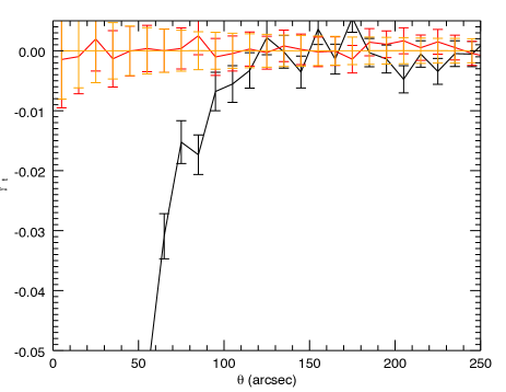
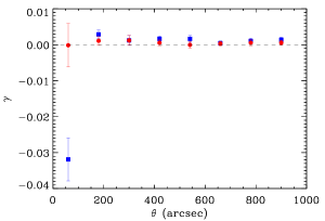
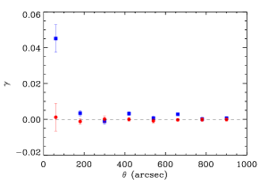
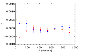
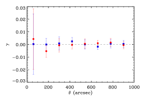
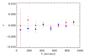
The measurements of the tangential and rotated distortion resulting from these tests are shown in the left panel of Fig. 1 and reveal a strong negative tangential (i.e. radial) distortion signal $\widehat{\gamma}_{t}(\theta)$, on scales $\theta\lesssim 200^{\prime\prime}$.

Figure 1: Tests for spurious distortions in the measured ellipticities of the FIRST background sources. The tangential shear, estimated using equation (16), for a “lens” sample consisting of radio sources in the FIRST catalogue, is shown as the cyan crosses. A large radial systematic signal is apparent. From left to right, the three panels show the results when all the FIRST radio sources are used as the “lens” sample (left), and randomly selecting 25 % (centre) or 10 % (right) of the FIRST sources respectively. The residual tangential and rotated shear after applying the correction described in Section 5 are shown as the blue squares and red circles respectively.

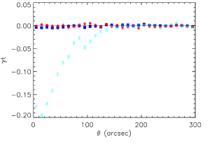
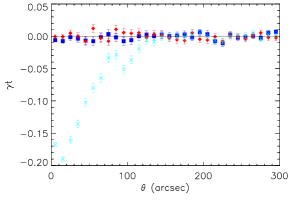
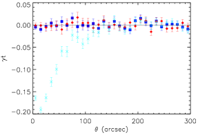
The measured rotated signal $\widehat{\gamma}_{r}(\theta)$, is consistent with zero. Though noisier, the radial distortion signal persists if we randomly select a subset of the FIRST objects as the “lens” sample (middle and right panels of Fig. 1). Furthermore we have confirmed that the measured signal shows no dependancy on the flux or size of the objects used to construct either the lens or source samples.

To investigate further, Fig. 2 shows the tangential and rotated distortion measured from the same sample as used in Fig. 1 but now plotted as $\gamma_{t}(\mn@boldsymbol{\theta})$ and $\gamma_{r}(\mn@boldsymbol{\theta})$ where $\mn@boldsymbol{\theta}=(\Delta RA,\Delta\delta)$ is the 2-D displacement vector from the central lens positions.

Figure 2: Maps of the spurious tangential shear ($\gamma_{t}(\mn@boldsymbol{\theta})$, left panel) and rotated shear ($\gamma_{r}(\mn@boldsymbol{\theta})$, right panel) as a function of the 2-D displacement of the FIRST selected sources from central lens positions for the case where the “lens” sample is composed of all sources in the FIRST catalogue. The upper (lower) panels show the measured distortion before (after) application of the correction described in Section 5 respectively.

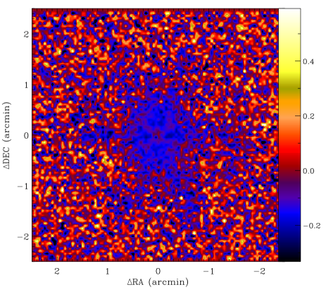
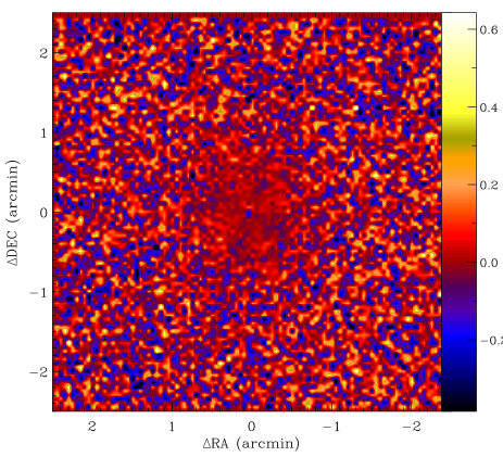
This figure shows that the measured radial distortion signal resembles the 6-arm shape of the synthesised beam (or PSF) of the VLA telescope in “snap-shot mode” which was the observation mode that was employed for the collection of the FIRST data. Once again the rotated shear signal is found to be consistent with zero. The results clearly show that the signal is of artificial origin and therefore the shapes need further correction. The results also suggest that the measured systematic is associated with an imperfect deconvolution and/or CLEANing of the sources during the imaging stage of the FIRST data reduction.

These detected ellipticity distortions would most likely bias a galaxy-galaxy or galaxy-cluster lensing analysis. We therefore apply a correction to the shapes of the FIRST galaxies based on the spurious negative tangential shear signal detected in Fig. 1. To apply the correction, we assume that the detected $\gamma_{t}(\theta)$ signal in the shape of each galaxy is due to an additive instrumental systematic effect caused by the presence of all of the other sources in the FIRST data (this would be the case if the origin of the systematic were an imperfect deconvolution of the FIRST synthesised beam). In that case, for the $i^{th}$ galaxy in the sample of FIRST background objects, we can estimate the total contribution to its measured ellipticity from instrumental systematic effects as

$$\epsilon_{1,i}^{\mathrm{sys}} \approx \sum_{j}\gamma_{t}^{\mathrm{sys}}(\theta_{ij})\cos(2\omega_{ij}),$$ (35)

$$\epsilon_{2,i}^{\mathrm{sys}} \approx \sum_{j}\gamma_{t}^{\mathrm{sys}}(\theta_{ij})\sin(2\omega_{ij}),$$ (36)

where the sum is over all sources in the FIRST catalogue. $\omega_{ij}$ is the angle between the reference axis of the $\epsilon_{1/2}$ coordinate system and the line joining the $i^{th}$ galaxy in the FIRST background sample with the $j^{th}$ galaxy in the FIRST catalogue. $\gamma_{t}^{\rm sys}(\theta_{ij})$ is the systematic tangential shear (plotted as the cyan points in the left-hand panel of Fig. 1) and $\theta_{ij}$ is the angular separation between the $i^{th}$ galaxy in the FIRST background sample and the $j^{th}$ galaxy in the FIRST catalogue. The FIRST shapes are then corrected simply by subtracting the systematic signals, estimated using equations (35) & (36), from the uncorrected galaxy ellipticities as listed in the FIRST catalogue.

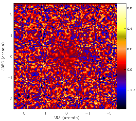
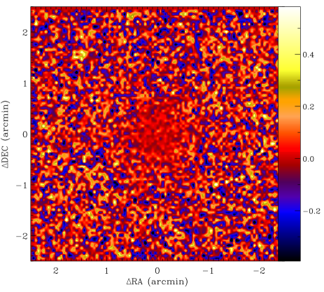
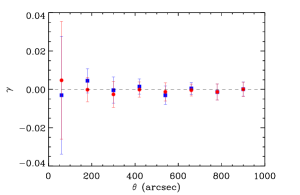
The success of the correction algorithm was assessed by repeating the diagnostic tests described above but now using the corrected ellipticities. The results, shown in Fig. 1 and Fig. 2, indicate that the correction has successfully removed the systematic radial distortions that were previously present in the FIRST shapes.

The approach that we have used to estimate the instrumental systematics will be sensitive, to a small extent, to any real galaxy-galaxy lensing signal present in the data. This is because the FIRST source population is extended in redshift space and therefore some of the sources will be lensed by others in the sample. We note that if this effect is present at a significant level, then it is likely to dilute the radial distortion caused by the instrumental systematics, thus leading to an under-correction of the systematic effects.

6 Simulations

As mentioned above, our procedure for correcting the FIRST galaxy shapes for residual instrumental distortions will be sensitive, to a small extent, to any real galaxy-galaxy lensing signal present in the data. In this section, we use simulations to assess the extent of the resulting bias in a subsequent galaxy-galaxy lensing study based on the corrected shapes. The simulations are also used to further examine the contamination removal method that was applied to the FIRST data and to estimate the uncertainties in the measurement due to random shape noise in the FIRST galaxies.

In order to generate the signal component of our simulations, we follow the general procedure described in Section 5 of Demetroullas & Brown (2016) and model both the overdensity and shear signals as correlated Gaussian random fields. Denoting overdensity fields as traced by the FIRST and SDSS galaxy positions as $G_{f}$ and $G_{s}$ respectively, and the convergence field extracted from the FIRST shear measurements as $\kappa_{f}$, we can model the 2-point statistics of these fields using the following power spectrum matrix:

$$\mathbf{C}_{\ell}=\left(\begin{array}[]{ccc}C^{G_{f}G_{f}}_{\ell}&C^{G_{f}\kappa_{f}}_{\ell}&C^{G_{f}G_{s}}_{\ell}\\ C^{\kappa_{f}G_{f}}_{\ell}&C^{\kappa_{f}\kappa_{f}}_{\ell}&C^{\kappa_{f}G_{s}}_{\ell}\\ C^{G_{s}G_{f}}_{\ell}&C^{G_{s}\kappa_{f}}_{\ell}&C^{G_{s}G_{s}}_{\ell}\end{array}\right).$$ (37)

Note that we do not need to include correlations involving the convergence field extracted from SDSS shear measurements ($\kappa_{S}$) in equation (37) as in this study we are not making use of SDSS galaxy shapes. We then make the further simplifying assumption that the overdensity field as traced by the FIRST galaxy positions is not correlated with either of the other fields, in which case the power spectrum matrix becomes:

$$\mathbf{C}_{\ell}=\left(\begin{array}[]{ccc}C^{G_{f}G_{f}}_{\ell}&0&0\\ 0&C^{\kappa_{f}\kappa_{f}}_{\ell}&C^{\kappa_{f}G_{s}}_{\ell}\\ 0&C^{G_{s}\kappa_{f}}_{\ell}&C^{G_{s}G_{s}}_{\ell}\end{array}\right).$$ (38)

In reality there will be some correlation between the FIRST and SDSS galaxy positions ($C^{G_{f}G_{s}}_{\ell}\equiv C_{\ell}^{G_{s}G_{f}}\neq 0$) since the redshift distributions of these two samples do overlap (and indeed there are $\sim 78000$ galaxies common to both catalogues). Similarly, there could also be a small correlation between the FIRST galaxy positions and the convergence field as extracted from the FIRST shear measurements ($C^{G_{f}\kappa_{f}}_{\ell}\equiv C_{\ell}^{\kappa_{f}G_{f}}\neq 0$) due to lensing of background FIRST sources by foreground FIRST sources. However, we expect both of these terms to be small and, in any case, we are including the most important cross-correlation for the purposes of the current study — that between the convergence field as extracted from the FIRST shear measurements and the SDSS galaxy positions ($C_{\ell}^{G_{s}\kappa_{f}}\equiv C_{\ell}^{\kappa_{f}G_{s}}$). It is this latter correlation that gives rise to a galaxy-galaxy (or cluster-galaxy) tangential lensing signal that is measurable by stacking the shapes of background FIRST galaxies around the positions of SDSS foreground objects.

We generate the entries of the power spectrum matrix (equation 38) based on a $\Lambda$CDM cosmology using equations (5), (8) and (11). For these calculations, we adopt the same cosmological parameters as listed in Section 5 of Demetroullas & Brown (2016) and we assume median redshifts of $z^{\rm{SDSS}}_{\rm{m}}=0.53$ and $z^{\rm{FIRST}}_{\rm{m}}=1.2$ for the SDSS and FIRST samples respectively. (See Fig. 8 in Demetroullas & Brown 2016 for the adopted redshift distributions). For all of our simulations we assume that the galaxy distribution traces the dark matter distribution perfectly ($r_{g}$=$b_{g}$=1). Once generated the power spectrum matrix is then used to produce correlated realisations of the shear and over-density fields within the healpix framework (Górski et al., 2005) for the two surveys following the procedure outlined in Section 5.1 of Demetroullas & Brown (2016).

In order to probe the angular scales on which the residual distortions in the FIRST data have been detected (see Fig. 1), the simulated maps are generated at a healpix resolution of nside = 8192, corresponding to a sky pixel side length $\simeq\,25$ arcsec. The simulated over-density fields for the two surveys are used to assign mock positions to 38.5 million SDSS and $2.7\times 10^{5}$ FIRST sources. Note that this analysis, contrary to Demetroullas & Brown (2016), makes use of only the positions of the SDSS sources and not their shapes. Therefore all 38.5 million sources are included in the simulation.

For the FIRST survey we also generate a mock galaxy shape catalogue as follows. Each FIRST simulated source is assigned ellipticity components based on the values, at the appropriate sky location, in the corresponding simulated shear map. Intrinsic shape noise is included by adding a real FIRST galaxy ellipticity measurement, randomly selected from the FIRST catalogue. The systematic errors in FIRST induced by the VLA beam residuals are modelled as described in Section 5.3 of Demetroullas & Brown (2016). Briefly, we first generate a template of the spurious negative tangential shear signal that was measured in the FIRST data (Fig. 9 in Demetroullas & Brown 2016). The template is normalised such that the amplitude of its azimuthicaly averaged tangential shear signal matches the amplitude of the signal shown in the left panel of Fig. 1. The normalized template is then used to generate additional spurious ellipticity contributions which we add to the entries in our simulated mock shape catalogue. For any one galaxy, these additional contributions model the contamination due to the sidelobes of all of the other sources in the data and are constructed from the normalized template according to equations (35)–(36).

We create 100 simulated data-sets according to the above prescription, each one containing a known galaxy-galaxy lensing signal and random ellipticity noise due to the intrinsic shapes of the FIRST sources. In each case we choose to store the information on the FIRST shapes prior to and after the addition of our model for the instrumental contamination. This allows us to assess the probable impact of the residual beam effects on the measured galaxy-galaxy lensing signal.

6.1 Simulated Source Shape Corrections

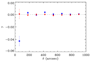
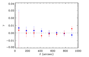
Having created mock galaxy position and shear catalogues which include a known galaxy-galaxy lensing signal, we then process the simulated data in exactly the same way as used for the analysis of the real data. The first step is to correct the mock FIRST galaxy shapes for the effects of the spurious radial distortion signal that was included in our simulations. We perform this correction as described in Section 5, constructing an estimate of the systematic signal by stacking the shapes of the FIRST sources around the positions of the FIRST sources. The resulting template is then used to correct the entries in the mock shape catalogues for the systematic effect. A demonstration of this correction at work on one of our simulations is presented in Fig. 3, which shows a radial systematic signal similar to that found in the real data (Fig. 1) being successfully removed by our correction algorithm.

Figure 3: The measured contamination from a random simulation. The black, orange and red solid lines represent the measured tangential signal before (black points) and after (orange points) the simulated FIRST sources shapes were corrected and the measured rotated shear after the shape correction (red points).

6.2 Galaxy-Galaxy Lensing Signal from Simulations

We proceed to measure the galaxy-galaxy lensing signal by correlating the positions of the SDSS objects with the shapes of the FIRST sources in the mock catalogues. Before doing so however, we point out a number of modifications that need to be applied to the theoretical prediction for a self-consistent analysis.

Firstly, we note that by imprinting a known theoretical $C_{\ell}^{G\kappa}$ signal onto a pixelised map, its shape is altered. To account for the effect of the pixelisation, we must include its smoothing effect on the input power spectrum; that is, we consider the effective input power to be $F_{\ell}^{2}C_{\ell}^{G\kappa}$, where $F_{\ell}$ is a known function describing the smoothing effects of the pixelisation used in the healpix maps.

Secondly, we note the limitations of our simulations in approximating both the shear and galaxy overdensity fields as Gaussian random fields (GRFs) and that this is not a very good model, in particular for the overdensity field. Defining the galaxy overdensity field as

$$\delta=\frac{N-\bar{N}}{\bar{N}}~{},$$ (39)

where $N$ is the number of galaxies in a map pixel and $\bar{N}$ is the mean galaxy occupation number in a pixel, averaged across all map pixels, we note that $\delta$ values constructed from a galaxy position catalogue according to equation (39) must lie in the range $-1\leq\delta\leq\delta^{\prime}_{\rm max}$, where $\delta^{\prime}_{\rm max}$ is some arbitrary maximum value. (The lower limit is $-1$ since the minimum number of galaxies that can be contained within a single pixel is $N=0$). However, for a given set of theory model power spectra ($C_{\ell}^{G_{f}G_{f}},C_{\ell}^{G_{s}G_{s}},C_{\ell}^{G_{s}\kappa_{f}}$, ), our GRF simulations produce overdensity values in some other (symmetric) range $-\delta_{\rm max}\mathrel{\hbox to0.0pt{\lower 4.0pt\hbox{\hskip 1.0pt$\sim$}\hss}\raise 1.0pt\hbox{$<$}}\delta\mathrel{\hbox to0.0pt{\lower 4.0pt\hbox{\hskip 1.0pt$\sim$}\hss}\raise 1.0pt\hbox{$<$}}\delta_{\rm max}$, where $\delta_{\rm max}$ is a non-unity number which is determined by the amplitude of the model power spectra.

To account for this discrpeancy and to properly connect our input theoretical models with the galaxy-galaxy lensing statistics which we measure from the simulated catalogues, we re-calibrate the simulated overdensity fields by a factor $1/\delta_{\rm max}$ so that they lie in the range $-1\mathrel{\hbox to0.0pt{\lower 4.0pt\hbox{\hskip 1.0pt$\sim$}\hss}\raise 1.0pt\hbox{$<$}}\delta\mathrel{\hbox to0.0pt{\lower 4.0pt\hbox{\hskip 1.0pt$\sim$}\hss}\raise 1.0pt\hbox{$<$}}1$. This allows us to populate the map pixels in a self-consistent way so that the galaxy population of every map pixel is strictly $\geq 0$ as required, subject to the constraint that the total number of lens galaxies in the simulation is kept fixed at the true value of $N^{\rm SDSS}_{\rm gal}=38.5$ million. Our final theoretical prediction for the galaxy-galaxy lensing signal as measured from the scaled simulation, and also taking into account the pixelisation smoothing is then simply (c.f. equation 14)

$$\gamma_{t}(\theta)=\frac{1}{2\pi\delta_{\rm max}}\int_{0}^{\ell_{\rm max}}\ell\mathrm{d}\ell F_{\ell}^{2}C_{\ell}^{G\kappa}J_{2}({\ell\theta})~{},$$ (40)

where $\ell_{\rm max}$ is the maximum multipole that was included in the simulation.

Figure 4: From left to right are the mean recovered tangential shear signal measured from 100 simulations in the absence (left panel) and presence (centre panel) of systematic effects, and after the FIRST simulated shapes were corrected (right panel). Over-plotted as the red line in each case is the predicted tangential signal (equation 40).

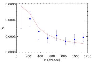
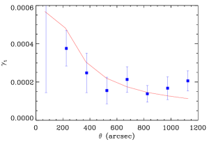
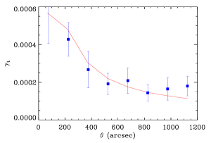
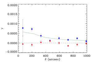
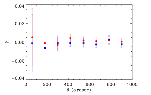
Fig. 4 shows the tangential weak lensing shear signal recovered in the absence (left panel) and in the the presence (centre panel) of the simulated FIRST systematics, and after shape corrections were applied (right panel), averaged over the 100 Monte-Carlo (MC) simulations that we have performed. The three panels show a very similar picture, although the points in the measurement that was made using the uncorrected FIRST shapes seem to have a slightly larger scatter around the predicted theory curve. However, in all three cases, the measured tangential shear is consistent with the input signal, while the rotated shear (not shown) was found to be consistent with zero.

We note that the unbiased recovery that we observe in our simulations is, in part, due to the fact that we do not include any position correlations between our two simulated galaxy samples. This means that the spurious position-shape correlations that were included in the mock FIRST data will not propagate to the cross correlation measurement between the simulated SDSS galaxy positions and the simulated FIRST galaxy shapes. The cross-correlation tangential shear signal in the presence of these small scale systematics in FIRST is consequently unbiased and therefore the correction step does not improve the outcome.

Finally, we note that the uncertanties (which are calculated from the run-to-run scatter amongst the 100 MC simulations) in all three cases are also very similar. This is because at this point the results are dominated by statistical errors due to the random intrinsic dispersion in the FIRST galaxy shapes. Further investigation of this matter has shown that by increasing the number of FIRST or SDSS sources (and therefore decreasing the statistical uncertainties), the additional scatter induced by the modelled contamination in the data is no longer negligible (the error bars increase by a few percent).

7 Real Data Measurements

In the previous section we have used simulations (which include a model of the VLA beam systematics) to demonstrate that our analysis pipeline is able to successfully recover a known galaxy-galaxy lensing signal that was injected into the simulated FIRST galaxy shapes. We now apply the same analysis pipeline to the real data. To estimate the uncertainties in our measurements we once again use the scatter in the MC simulations.

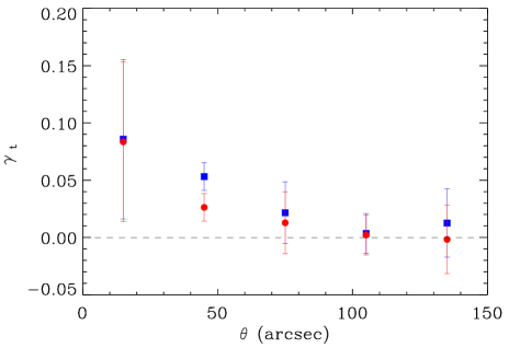
The galaxy-galaxy lensing signal measured from the real data (by stacking the shapes of the FIRST galaxies around the positions of the SDSS galaxies) is shown in the left hand panels of Fig. 5. When comparing the signals before and after correcting the FIRST shapes (top and bottom panels respectively) one can see that the FIRST beam systematic effect has corrupted the tangential shear signal on scales $\theta\lesssim 200$ arcsec, while the rest of the data points (both for $\gamma_{t}$ and $\gamma_{r}$) are almost unchanged. A similar picture emerges for the cases where we consider the other two lens samples (i.e. the BCG and SDSS-FIRST matched samples – these are shown in the centre and right hand panels of Fig. 5 respectively). We note that on application of our correction algorithm for the FIRST shape systematics, the detected signal on scales $\theta<200$ arcsec changes from a strong radial distortion signal (which is consistent with being caused by the spurious systematics already identified in the FIRST data) to a tangential distortion signal after correction that is broadly consistent with theoretical expectations.

We find the tangential shear measurement made using the FIRST corrected shapes for scales of $0\leq\theta\leq 1200$ arcsec, to be inconsistent with zero at the $\sim 10\sigma$ level. To assess the degree with which the measured signal is in agreement with the cosmological model we calculate the $\chi^{2}$ misfit statistic as

$$\chi^{2}=\sum_{b}(\hat{\gamma}_{b}^{t}-\gamma_{b}^{t,\rm th})^{2}/\sigma^{2}_{\hat{\gamma}_{b}^{t}},$$ (41)

where $\gamma^{t,\rm th}_{b}$ is the expected value of the tangential shear in a given angular separation bin $b$ and $\sigma_{\hat{\gamma}_{b}^{t}}$ is the errorbar calculated using the scatter in the measurements of the equivalent angular separation bin amongst the MC simulations. For scales $\theta\mathrel{\hbox to0.0pt{\lower 4.0pt\hbox{\hskip 1.0pt$\sim$}\hss}\raise 1.0pt\hbox{$>$}}200$ arcsec we convert the misfit statistics to likelihood values for a model with two degrees of freedom, the median redshift of the FIRST and SDSS surveys. We find that the measured signal is in agreement with the theoretical predictions for a Planck cosmology and two galaxy populations with median redshifts, $z^{\rm{SDSS}}_{\rm{m}}=0.53$ and $z^{\rm{FIRST}}_{\rm{m}}=1.2$ at the 2$\sigma$ level. We omit the measurements in the two lowest $\theta$-bins from the analysis as the adopted Gaussian model for the galaxy-galaxy lensing signal is unlikely to be valid on these small scales. Finally for the main SDSS lens sample, we find that the rotated shear signal is consistent with zero.

Figure 5: The measured tangential (blue squares) and rotated (red circles) shear using as lenses the SDSS complete catalogue (left panels), the BCG sample (centre panels) and the sample composed of the SDSS-FIRST matched objects (right panels). The upper panels show measurements using the uncorrected FIRST galaxy shapes while the lower panels show the results after the shape corrections were applied. Over-plotted in the left panels is the theoretical tangential shear signal for a set of foreground and background sources lying at redshifts of $z^{1}_{\mathrm{median}}$=0.53 and $z^{2}_{\mathrm{median}}$=1.2 respectively.

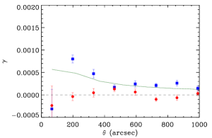
For the other two lens samples, we also measure a tangential shear signal that is inconsistent with zero: at $3.8\sigma$ for the BCG sample and at 9$\sigma$ for the FIRST-SDSS matched galaxy lens sample (shown in the upper centre and upper right panels of Fig. 5 respectively). The rotated shear signal for the SDSS-FIRST matched galaxy lens sample is consistent with zero. The measured rotated shear for the BCG lens sample, although lower than the measured tangential shear, is inconsistent with zero. As expected, the tangential shear measured around the BCG lens sample is $\sim$1 order of magnitude larger than that measured using the main SDSS DR10 catalogue. Perhaps unexpectedly though, the shear signal detected around the SDSS-FIRST matched objects is even higher than that measured around the BCGs. It also appears to have the steepest slope out of the three cases as it becomes consistent with zero for scales $\theta\gtrsim 150$ arcsec. This scale, assuming a median redshift for the lens sample of $z^{\rm matched}_{\rm m}$=0.57, corresponds to a radius of $R\simeq 1$ Mpc.

7.1 Residual Systematics Test Measurements

To further assess the validity of the results we perform a set of measurements on the real data which are designed to reveal residual systematics that may remain in the data after application of our correction algorithm. For all of these measurements we assign errorbars by processing the simulated datasets in exactly the same way as the real data and then calculating the scatter in the measurements from the MC simulations.

We have performed the following null tests for each of the three lens samples that we have considered:

1. North-South: we split the lens sample and the FIRST data into roughly equal North and South samples. We then measure the galaxy-galaxy lensing signal from each sample separately. Finally, we subtract the signal between the two measurements.

2. East-West: Same as test (i) but splitting the data into a West and an East component.

3. Random lens: Randomly splitting the lens samples into two equal subsets. For each subset the galaxy-galaxy lensing signal is measured. Finally we subtract the two measurements.

4. Random lens position: We randomly select positions on the sky to match the number of lenses in each lens group. We then use those positions as central stacking points and measure the mean stacked galaxy-galaxy lensing signal around those points.

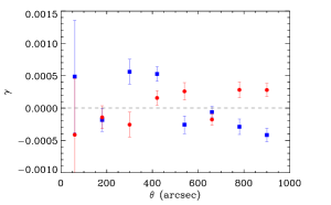
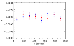
The results of these tests are shown in Fig. 6. In all cases the results, both in the tangential and the rotated direction, are consistent with zero. The scatter of the points both for the tangential and the rotated shear signal for the North-South test conducted on the SDSS full sample seems to be larger than for the rest of the tests, but still no obvious coherent signal could be detected. The tests therefore reveal no major issues with the analysis that was followed.

Figure 6: Form left to right are the null tests conducted using the full SDSS sample (left panels), the BCG lens sample (centre panels) and the lens sample composed of the SDSS-FIRST matched objects (right panels). From top to bottom the panels show the North-South, West-East, Random lens and Random lens position tests respectively. Blue squares and red circles show the measured tangential and rotated shear respectively.

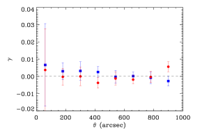
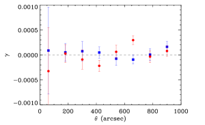
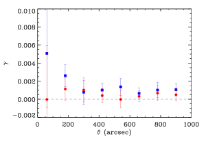
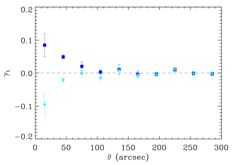
In addition to these null tests we have also looked into the redshift dependence of the signal that was measured using the SDSS-FIRST matched objects and the FIRST shapes. In this test we look on angular scales where there is a significant non-zero tangential shear signal ($\theta<150$ arcsec). We compare the measured tangential shear signal around the SDSS-FIRST sources that have redshifts $z_{low}<1$ and $z_{high}>1$. The results (see Fig. 7) although noisy, suggest that the signal decreases when one changes lens samples from the low-redshift sub-sample to the high-redshift sub-sample. This is consistent with the expected behaviour for a real shear signal for which the strength of the signal is expected to decrease as a function of the lens redshifts.

Figure 7: The tangential shear signal measured using the FIRST selected sources as background objects and the SDSS-FIRST matched objects with $z_{low}<1$ (blue squares) and $z_{high}>1$ (red circles) as lenses.

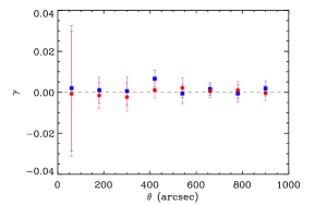
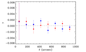
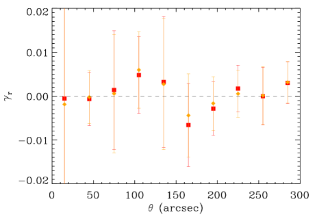
Finally, we look at the signal dependence as a function of angular scale $\theta$ before and after shape corrections for when the SDSS-FIRST matched objects are used as lenses. We primarily focus on this sample because a galaxy-galaxy lensing measurement, made by stacking the FIRST shapes around the positions of this group, will more likely be biased if the shape correction algorithm was not successful (since all of the lenses in this sample are bright in the radio). The results of this invesitgation are shown in Fig. 8. As expected, the tangential shear signal for this lens group prior to correcting the shapes of the FIRST sources is negative for $\theta\leq 200$ arcsec. This signal, although negative in absolute value, is smaller in amplitude than the spurious signal detected when the complete FIRST catalogue was used as central objects (see left panel of Fig. 1). This suggests that a strong positive cosmological tangential shear is also present competing with the spurious negative one. The measured tangential component of the shear after shape corrections are applied is positive but has a steep slope as it becomes consistent with zero for $\theta\mathrel{\hbox to0.0pt{\lower 4.0pt\hbox{\hskip 1.0pt$\sim$}\hss}\raise 1.0pt\hbox{$>$}}150$ arcsec. The measured rotated shear signals for the two cases are consistent with each other and they are also consistent with zero (see right panel of Fig. 8). All of these tests show no obvious evidence of residual systematics in the data after the shape correction step was performed.

Figure 8: Galaxy-galaxy lensing measurements using the SDSS-FIRST matched objects as lenses and the selected FIRST sources as background objects. The tangential shear prior to (cyan circles) and after shape corrections (blue squares) is shown in the left panel and the rotated shear prior to (orange circles) and after shape corrections (red squares) is shown in the right panel.

7.2 Constraints on the Properties of the Lensing Sources

Having demonstrated the credibility of our results we now fit the two dark matter halo models described in Section 3 to the measured tangential shear to constrain the ensemble mass $M_{200}$, the radius $R_{200}$, the velocity dispersion $\sigma_{u}$ and the Einstein radius $\theta_{\mathrm{E}}$ for each of the lens samples that we have investigated. To fit the data both models should be provided with the median redshifts of the lens and background source populations. Additionally, for the NFW model, the lens concentration factor can either be supplied or left to be constrained by the data. Initially we choose to adopt the value for this parameter drawn from Bullock et al. (2001). Subsequently we allow the concentration factor to vary and we compare the returned $\chi^{2}$ and parameter values. The values for the sources’ redshifts and concentration factors that were extracted from the literature to fit the three detected shear signals are summarised in Table 1.

Table 1: The lens and background objects redshifts and concentration factor values used to fit the data.

	SDSS	BCGs	SDSS-FIRST
$z_{\rm{lens}}$	0.53	0.37	0.57
$z_{\rm{BGsources}}$	1.2	1.2	1.2
$c_{f}$	10	7	7

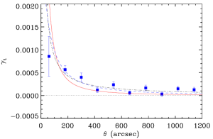
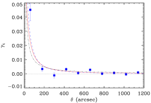
The tangential shear signal measured using the FIRST sources as background objects and the three lensing samples are shown in Fig. 9. Over-plotted are the best-fitting SIS and NFW models in which the parameters that were used are drawn from the literature. Also over-plotted is the best-fitting NFW model where the concentration factor is fitted from the data. The best-fitting parameters as determined by the data are listed in Table 2.

For the SDSS DR10 sample (left panel of Fig. 9) it is clear that the SIS model is more consistent with the data than the NFW model in which archival values for the concentration factor were used. Instead, when the concentration parameter is allowed to vary, the $\chi^{2}$ value for the fit decreases by $\sim$25. The results suggest that the NFW model can be used to constrain the halo mass of galaxies, but it will predict a mass profile for these sources that is much shallower than theoretically expected for $\sim$10¹² $\mathrm{M}_{\odot}$ objects. However, both models appear to predict broadly the same values for the enclosed mass of the sample $M_{200}$. The extracted values for the SDSS DR10 sample are consistent (within 1$\sigma$) with results from the Canada France Hawaii Lensing Survey (CFHTLenS). Velander et al. (2014) measured an Einstein radius and a velocity dispersion for the complete CFHTLenS lens sample of $\theta_{E}=0.136\pm 0.03$ and $\sigma_{u}=97.9\pm 1.0$ km s^-1 respectively. Also Parker et al. (2007) using a sub-set of that CFHTLenS sample measured an $M_{200}$ value of $M_{200}=1.1\pm 0.2\mathrm{M}_{\odot}$.

Figure 9: The measured tangential (blue squares) shear for the SDSS complete catalogue (left panel), the BCG sample (centre panel) and the SDSS-FIRST matched objects (right panel). Over-plotted are the best fitting NFW model with a fixed c_f (red continuous line), the best-fitting NFW model with a variable c_f (blue dashed line) and the best fitting SIS model (black dot-dashed line).

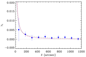
Both the SIS and the NFW profile, in which the concentration factor was drawn from the literature, are in good agreement with the shear signal measured from the BCGs (central panel of Fig. 9). Additionally, the best fit value for the concentration factor is roughly the same as the one drawn from Bullock et al. (2001). This is expected as the NFW profile is primarily used to predict the matter halos of galaxy clusters in which the dark matter is the predominant component. The extracted values for the BCG population are in good agreement with the Hubble Space Telescope (HST) STAGES study of the Abell 901/902 supercluster where cluster masses in the range $\left(3.5<M<6.5\right)\times 10^{13}$ M_⊙ h^-1 were measured (Heymans et al., 2008).

Using parameter values from the literature neither the SIS nor the NFW best fit models can accurately predict the tangential lensing signal that we have measured around the SDSS-FIRST matched object lens sample. When allowing the concentration factor to vary, the NFW model fits to a better degree the data ($\Delta\chi^{2}=2$) for the maximum allowed value for the parameter $c_{f}=12$. The predicted mass for these galaxies $M_{200}$ is of the order $10^{13}\mathrm{M}_{\odot}$. No similar work has been conducted on the SDSS-FIRST sample. Our findings suggest that galaxies, that are bright in both the optical and the radio, are embedded in very dense environments on scales $R\mathrel{\hbox to0.0pt{\lower 4.0pt\hbox{\hskip 1.0pt$\sim$}\hss}\raise 1.0pt\hbox{$<$}}1$ Mpc ($\theta\mathrel{\hbox to0.0pt{\lower 4.0pt\hbox{\hskip 1.0pt$\sim$}\hss}\raise 1.0pt\hbox{$<$}}150$ arcsec), a result that is in good agreement with a number of works in the literature (Balogh et al., 2004; Blanton et al., 2005, 2006).

Finally, it is illustrative to comment on the types of galaxies that make up the FIRST-SDSS matched catalogue sample. Masters et al. (2010) have shown that the SDSS catalogue parameter FRACDEV (which illustrates the fraction of light that is fitted by a de Vaucouleurs profile) can be used to separate early and late type galaxies. This is possible since early type elliptical and spirals with big bulges are traditionally better characterised by a de Vaucouleur profile and therefore have FRACDEV $>0.5$. Using the FRACDEV information in the SDSS data we find that the SDSS DR10 sample contains $\sim 60$% early type galaxies and $\sim 40$% late type galaxies. Contrary to this, in the SDSS-FIRST matched objects sample $\sim$85% of the galaxies are early type with only $\sim$15% late type. Courteau et al. (2014) showed by combining the results of a weak lensing, a strong lensing and a dynamic analysis study that early type SLACS galaxies in the redshift range $0.1<z<0.8$ have an average mass of $M\simeq 2\times 10^{13}M_{\odot}$. Our results for the masses of the FIRST-SDSS lens sample (which are predominantly early-type galaxies) are in good agreement with the findings of this study (within 2$\sigma$).

Table 2: Best-fitting parameters for the NFW and SIS dark matter halo models, as constrained by the tangential shear measurements around the thress lens samples.

		SDSS DR10		BCGs		SDSS-FIRST
NFW	$c_{f}$ fixed/fitted by the data	10	1	7	6	7	12
	$\chi^{2}$	40	15	5.2	5.0	27	25
	$r_{200}[Mpc]$	0.31$\pm$0.04	0.22$\pm$0.03	0.51$\pm$0.19	0.50$\pm$0.18	0.90$\pm$0.16	0.90$\pm$0.16
	$M_{200}$ [$\times 10^{12}$$M_{\odot}$]	3.2$\pm$1.3	1.2$\pm$0.4	15$\pm$14	14$\pm$13	79$\pm$43	80$\pm$42
SIS	$\chi^{2}$	15.5		4.5		31
	$\theta_{E}$ [arcsec]	0.17$\pm$0.02		0.92$\pm$0.25		1.89$\pm$0.32
	$\sigma_{u}$ [KM/h]	102$\pm$33		294$\pm$154		339$\pm$140
	$M_{200}$ [$\times 10^{12}$$M_{\odot}$]	1.3$\pm$0.2		32$\pm$13		48$\pm$15

8 Conclusions

In this study we have performed galaxy-galaxy and galaxy-cluster lensing analyses, combining information from the ovelapping optical SDSS and radio VLA-FIRST surveys.

The motivation for this work was to illustrate the advantages of using radio data in shear studies but also to show the additional benefits of cross correlating them with information in the optical. The VLA FIRST shapes were found to contain systematics that, unless accounted for, will most likely bias a radio-only shear study on angular scales $\theta\lesssim 200$ arcsec. By cross-correlating the shapes of selected FIRST sources with the positions of all FIRST sources we have detected a negative tangential shear which is a function of the angular separation between the FIRST galaxies and which is inconsistent with zero at the $>10\sigma$ level. The rotated shear signal was found to be consistent with zero. Further investigation revealed that the negative tangential shear resembles the shape of the VLA beam (or PSF) for observations conducted in snap shot mode, indicating that the signal is of artificial origins. From the azimuthally averaged negative tangential shear signal, we constructed a template of the systematic effect, which we then used to correct the original FIRST shapes.

Using simulations we showed that the cross correlation SDSS-FIRST galaxy-galaxy lensing signal is mostly unaffected by this type of systematic. However, we note that our simulations are not fully representative of the data as they did not include any correlations between the postions of the FIRST and SDSS galaxies. Such correlations exist to some degree in the real data and further analysis has shown that in the presence of these correlations, the shape systematis do impact the cross-correlation galaxy-galaxy lensing measurement, thus motivating the shape correction step that we have applied.

By cross correlating the positions of the SDSS DR10, BCG and SDSS-FIRST matched objects with the shapes of the FIRST selected sources, we measure a tangential shear signal that is inconsistent with zero at the $\sim 10\sigma$, $\sim 3.8\sigma$ and $\sim 9\sigma$ level respectively. At the same time in all three cases the detection significance of the rotated shear is much lower. The results are further assessed using a set of measurements designed to reveal any residual systematics in the data. These tests do not show any obvious leftover contamination in the data.

The shape of the measured tangential shear using the SDSS DR10 and FIRST sources on scales $\theta\gtrsim 200$ arcsec is compared to the signal predicted in a concordance cosmological model, assuming median redshifts for the SDSS DR10 and FIRST populations of $z^{\mathrm{SDSS}}_{m}$=0.53 and $z^{\mathrm{FIRST}}_{m}$=1.2 respectively. Our measurements agree within 2$\sigma$ with the theoretical predictions.

We also fitted our galaxy-galaxy lensing measurements using both NFW and SIS halo models. In doing so we found that both the SIS and the NFW profiles fit equally well the BCG-FIRST tangential shear signal. The concentration factor parameter in the NFW model that was extracted from the literature and the one fitted using our measurements are in good agreement. The tangential shear from the SDSS DR10 sample can be fitted relatively well using an SIS profile. The NFW profile can also fit the data at the same level but only if one allows the concentration factor to vary. However, the best fitting NFW profile is much shallower than the values quoted in the literature. The lensing signal measured around the SDSS-FIRST matched objects is best fitted with an NFW profile in which the concentration factor is much greater than what is typically quoted in the literature.

The best-fitting Virial mass $M_{200}$, Einstein radius $\theta_{\mathrm{E}}$ and velocity dispersion $\sigma_{u}$ for the SDSS DR10 and BCG samples agree within 1$\sigma$ with the values quoted in the literature. However, we find that the measured ensemble mass of the SDSS-FIRST matched galaxies is $\sim$2 orders of magnitude greater than the one found for the SDSS DR10 sample. Using the FRACDEV parameter in the SDSS catalogue we find that $\sim$85% of the SDSS-FIRST objects are early type galaxies while only $\sim$60% of the objects in SDSS DR10 belong to the same category. Courteau et al. (2014) has also showed that early type SLACS galaxies in the redshift range $0.1<z<0.8$ have an average mass of $M\simeq 2\times 10^{13}M_{\odot}$, a result that agrees with our findings at the 2$\sigma$ level. Our study has therefore shown that galaxies which are bright in both the optical and radio wavebands are typically embedded in very dense environments on angular scales of $R\mathrel{\hbox to0.0pt{\lower 4.0pt\hbox{\hskip 1.0pt$\sim$}\hss}\raise 1.0pt\hbox{$<$}}1$ Mpc.

References

- Ahn et al. (2014) Ahn, C. P., Alexandroff, R., Allende Prieto, C., et al., 2014, ApJS, 211, 17, arXiv:1307.7735
- Bahcall et al. (2003) Bahcall, N. A., Dong, F., Bode, P., et al., 2003, ApJ, 585, 182, astro-ph/0205490
- Balogh et al. (2004) Balogh, M., Eke, V., Miller, C., et al., 2004, MNRAS, 348, 1355, astro-ph/0311379
- Bartelmann & Schneider (2001) Bartelmann, M., Schneider, P., 2001, Phys. Rep., 340, 291, arXiv:astro-ph/9912508
- Becker et al. (1995) Becker, R. H., White, R. L., Helfand, D. J., 1995, ApJ, 450, 559
- Blanton et al. (2005) Blanton, M. R., Eisenstein, D., Hogg, D. W., Schlegel, D. J., Brinkmann, J., 2005, ApJ, 629, 143, astro-ph/0310453
- Blanton et al. (2006) Blanton, M. R., Eisenstein, D., Hogg, D. W., Zehavi, I., 2006, ApJ, 645, 977, astro-ph/0411037
- Blanton et al. (2003) Blanton, M. R., Hogg, D. W., Bahcall, N. A., et al., 2003, ApJ, 592, 819, astro-ph/0210215
- Bonaldi et al. (2016) Bonaldi, A., Harrison, I., Camera, S., Brown, M. L., 2016, ArXiv e-prints, arXiv:1601.03948
- Brainerd et al. (1996) Brainerd, T. G., Blandford, R. D., Smail, I., 1996, ApJ, 466, 623, astro-ph/9503073
- Brown et al. (2015) Brown, M., Bacon, D., Camera, S., et al., 2015, Advancing Astrophysics with the Square Kilometre Array (AASKA14), 23, arXiv:1501.03828
- Bullock et al. (2001) Bullock, J. S., Kolatt, T. S., Sigad, Y., et al., 2001, MNRAS, 321, 559, astro-ph/9908159
- Camera et al. (2016) Camera, S., Harrison, I., Bonaldi, A., Brown, M. L., 2016, ArXiv e-prints, arXiv:1606.03451
- Chang et al. (2004) Chang, T.-C., Refregier, A., Helfand, D. J., 2004, ApJ, 617, 794, arXiv:astro-ph/0408548
- Courteau et al. (2014) Courteau, S., Cappellari, M., de Jong, R. S., et al., 2014, Reviews of Modern Physics, 86, 47, arXiv:1309.3276
- Demetroullas & Brown (2016) Demetroullas, C., Brown, M. L., 2016, MNRAS, 456, 3100, arXiv:1507.05977
- Dressler (1980) Dressler, A., 1980, ApJ, 236, 351
- Evrard et al. (2002) Evrard, A. E., MacFarland, T. J., Couchman, H. M. P., et al., 2002, ApJ, 573, 7, astro-ph/0110246
- Fukushige & Makino (2001) Fukushige, T., Makino, J., 2001, ApJ, 557, 533, astro-ph/0008104
- Górski et al. (2005) Górski, K. M., Hivon, E., Banday, A. J., et al., 2005, ApJ, 622, 759, astro-ph/0409513
- Gunn & Gott (1972) Gunn, J. E., Gott, J. R., III, 1972, ApJ, 176, 1
- Harrison et al. (2016) Harrison, I., Camera, S., Zuntz, J., Brown, M. L., 2016, ArXiv e-prints, arXiv:1601.03947
- Heymans et al. (2008) Heymans, C., Gray, M. E., Peng, C. Y., et al., 2008, MNRAS, 385, 1431, arXiv:0801.1156
- Hoekstra et al. (2003) Hoekstra, H., Franx, M., Kuijken, K., Carlberg, R. G., Yee, H. K. C., 2003, MNRAS, 340, 609, astro-ph/0211633
- Högbom (1974) Högbom, J. A., 1974, A&AS, 15, 417
- Hu & Jain (2004) Hu, W., Jain, B., 2004, Phys. Rev. D, 70, 4, 043009, astro-ph/0312395
- Joachimi & Bridle (2010) Joachimi, B., Bridle, S. L., 2010, A&A, 523, A1, arXiv:0911.2454
- Mandelbaum et al. (2006) Mandelbaum, R., Seljak, U., Cool, R. J., Blanton, M., Hirata, C. M., Brinkmann, J., 2006, MNRAS, 372, 758, astro-ph/0605476
- Massey et al. (2010) Massey, R., Kitching, T., Richard, J., 2010, Reports on Progress in Physics, 73, 8, 086901, arXiv:1001.1739
- Masters et al. (2010) Masters, K. L., Nichol, R., Bamford, S., et al., 2010, MNRAS, 404, 792, arXiv:1001.1744
- McKay et al. (2001) McKay, T. A., Sheldon, E. S., Racusin, J., et al., 2001, ArXiv Astrophysics e-prints, astro-ph/0108013
- Meneghetti (1997) Meneghetti, M., 1997, Introduction to Gravitational Lensing, Lecture scripts
- Moore et al. (1999) Moore, B., Ghigna, S., Governato, F., et al., 1999, ApJL, 524, L19, astro-ph/9907411
- Muxlow et al. (2005) Muxlow, T. W. B., Richards, A. M. S., Garrington, S. T., et al., 2005, MNRAS, 358, 1159, astro-ph/0501679
- Navarro et al. (1996) Navarro, J. F., Frenk, C. S., White, S. D. M., 1996, ApJ, 462, 563, arXiv:astro-ph/9508025
- Navarro et al. (1997) Navarro, J. F., Frenk, C. S., White, S. D. M., 1997, ApJ, 490, 493, astro-ph/9611107
- Newman & Penrose (1966) Newman, E. T., Penrose, R., 1966, Journal of Mathematical Physics, 7, 863
- Newman & Davis (2002) Newman, J. A., Davis, M., 2002, ApJ, 564, 567, astro-ph/0109130
- Parker et al. (2007) Parker, L. C., Hoekstra, H., Hudson, M. J., van Waerbeke, L., Mellier, Y., 2007, ApJ, 669, 21, arXiv:0707.1698
- Press & Schechter (1974) Press, W. H., Schechter, P., 1974, ApJ, 187, 425
- Sheldon et al. (2004) Sheldon, E. S., Johnston, D. E., Frieman, J. A., et al., 2004, AJ, 127, 2544, astro-ph/0312036
- Sheldon et al. (2009) Sheldon, E. S., Johnston, D. E., Scranton, R., et al., 2009, ApJ, 703, 2217, arXiv:0709.1153
- Sypniewski (2014) Sypniewski, A. J., 2014, Optimizing Photometric Redshift Estimation for Large Astronomical Surveys Using Boosted Decision Trees
- Tojeiro et al. (2013) Tojeiro, R., Masters, K. L., Richards, J., et al., 2013, MNRAS, 432, 359, arXiv:1303.3551
- Tunbridge et al. (2016) Tunbridge, B., Harrison, I., Brown, M. L., 2016, ArXiv e-prints, arXiv:1607.02875
- van Uitert et al. (2011) van Uitert, E., Hoekstra, H., Velander, M., Gilbank, D. G., Gladders, M. D., Yee, H. K. C., 2011, A&A, 534, A14, arXiv:1107.4093
- Velander et al. (2014) Velander, M., van Uitert, E., Hoekstra, H., et al., 2014, MNRAS, 437, 2111, arXiv:1304.4265
- Viana & Liddle (1999) Viana, P. T. P., Liddle, A. R., 1999, ArXiv Astrophysics e-prints, astro-ph/9902245
- Wen et al. (2012) Wen, Z. L., Han, J. L., Liu, F. S., 2012, ApJS, 199, 34, arXiv:1202.6424
- White et al. (1993) White, S. D. M., Efstathiou, G., Frenk, C. S., 1993, MNRAS, 262, 1023
- Wilman et al. (2008) Wilman, R. J., Miller, L., Jarvis, M. J., et al., 2008, MNRAS, 388, 1335, arXiv:0805.3413
- Wong et al. (2012) Wong, O. I., Schawinski, K., Kaviraj, S., et al., 2012, MNRAS, 420, 1684, arXiv:1111.1785
- Wright & Brainerd (2000) Wright, C. O., Brainerd, T. G., 2000, ApJ, 534, 34
- York et al. (2000) York, D. G., Adelman, J., Anderson, J. E., Jr., et al., 2000, AJ, 120, 1579, astro-ph/0006396