Damping of hard excitations in strongly coupled $\mathcal{N}\,{=}\,4$ plasma

Abstract

The damping of high momentum excitations in strongly coupled maximally supersymmetric Yang-Mills plasma is studied. Previous calculations of the asymptotic behavior of the quasinormal mode spectrum are extended and clarified. We confirm that subleading corrections to the lightlike dispersion relation $\omega({\bf q})=|{\bf q}|$ have a universal $|{\bf q}|^{-1/3}$ form. Sufficiently narrow, weak planar shocks may be viewed as coherent superpositions of short wavelength quasinormal modes. The attenuation and evolution in profile of narrow planar shocks are examined as an application of our results.

I Introduction

In a strongly coupled Yang-Mills plasma, such as that of maximally supersymmetric Yang-Mills ($\mathcal{N}\,{=}\,4$ SYM) theory, the typical time scale for relaxation of non-hydrodynamic perturbations is set by the inverse temperature $T^{-1}$. In a dual holographic description, this scale may be interpreted as the characteristic gravitational infall time for perturbations falling through the horizon of black brane geometries which describe near-equilibrium states Chesler and Yaffe (2009); Bhattacharyya and Minwalla (2009).

However, even in the strong coupling limit, sufficiently high momentum excitations are only weakly damped. This may, for example, be seen in the large wavenumber asymptotics of the quasinormal mode (QNM) spectrum. At zero temperature in $\mathcal{N}\,{=}\,4$ SYM, Fourier transformed two-point correlation functions, viewed as functions of frequency $\omega$ at fixed wavenumber ${\bf q}$, have branch cuts starting at the lightcone, $\omega=\pm|{\bf q}|$. At non-zero temperature, and in the $N\to\infty$ limit, this branch cut breaks up into a closely spaced series of poles at locations $\omega=\{\omega_{n}^{\pm}({\bf q})\}$ known as quasinormal mode frequencies Starinets (2002); Nunez and Starinets (2003); Kovtun and Starinets (2005). Festuccia and Liu Festuccia and Liu (2009) studied the large-${\bf q}$ asymptotics of the quasinormal mode spectrum for scalar perturbations (or helicity $\pm 2$ stress-energy perturbations) and found that as $|{\bf q}|\to\infty$,

$$\omega_{n}^{\pm}({\bf q})/|{\bf q}|\sim\pm\left[1+c_{n}\,e^{\mp i\pi/3}\,(\pi T/|{\bf q}|)^{4/3}\right],$$ (1)

with real “spectral deviation” coefficients $\{c_{n}\}$ which are discussed below. The small imaginary part (relative to the real part), $\mathop{\rm Im}\omega_{n}^{\pm}({\bf q})/\mathop{\rm Re}\omega_{n}^{\pm}({\bf q})={\mathcal{O}}(T/|{\bf q}|)^{4/3}$, demonstrates the weak damping for $|{\bf q}|\gg T$, and shows that these high energy, short wavelength excitations may, in some respects, be regarded as quasiparticles, i.e., excitations whose mean free path is much longer than their de Broglie wavelength. However, because $|{\bf q}|\gg T$, these are highly athermal excitations which are exponentially rare in equilibrium. Moreover, because the spacing in energy between successive quasinormal modes is comparable to their width, $|\omega_{n+1}^{\pm}({\bf q})-\omega_{n}^{\pm}({\bf q})|\sim|\mathop{\rm Im}\omega_{n}^{\pm}({\bf q})|$, the spectral densities of correlation functions, at large ${\bf q}$, do not have distinct narrow peaks in frequency associated with each quasinormal mode; instead the contributions of multiple QNMs merge to produce a slowly varying spectral density Steineder et al. (2013a).

The weak damping of high ${\bf q}$ excitations may also be seen in the behavior of planar shocks. At zero temperature, planar shocks propagate at the speed of light without dispersion or attenuation. At non-zero but low temperatures (small compared to the inverse width of the shock), the shock experiences weak thermal drag Chesler and Yaffe (2011). This slowly attenuates the amplitude of the shock and introduces dispersion, but this weak damping vanishes as $T\to 0$.

In this paper, we study the damping of high ${\bf q}$ excitations in $\mathcal{N}\,{=}\,4$ SYM theory in greater detail. In section II we perform our own WKB analysis of the large-${\bf q}$ asymptotics of helicity $\pm 2$ quasinormal mode frequencies. We confirm the relative $|{\bf q}|^{-4/3}$ form (1) of the leading corrections to a lightlike dispersion relation, with a universal $\mp\pi/3$ phase. However, we find values for the coefficients $\{c_{n}\}$ of these corrections which disagree in two respects with the result given in ref. Festuccia and Liu (2009), which was

$$c_{n}=K_{\rm FL}\,(2n+1)^{4/3}\,,\qquad n=1,2,\cdots,\qquad\mbox{[Festuccia \& Liu]}\,,$$ (2)

with $K_{\rm FL}=[\sqrt{\pi}\,\Gamma\big{(}\tfrac{7}{4}\big{)}/\Gamma\big{(}\tfrac{1}{4}\big{)}]^{4/3}=0.344127\cdots$. The $(2n+1)^{4/3}$ dependence on mode number is asymptotically correct for high-lying modes, but is not accurate for low order modes. Moreover, the coefficient $K_{\rm FL}$ differs by a factor of $2^{5/3}$ from the correct value in the large order asymptotic form,

$$c_{n} \sim K\,(2n+1)^{4/3}\,,\qquad n\gg 1\,,$$ (3a)

with

$$K =\tfrac{1}{2}[\sqrt{\pi}\,\Gamma\big{(}\tfrac{7}{4}\big{)}/\Gamma\big{(}\tfrac{5}{4}\big{)}]^{4/3}=1.092535\cdots\,.$$ (3b)

The need for a $2^{5/3}$ correction factor in the value of the coefficient $K_{\rm FL}$ for AdS₅ black holes was noted earlier in ref. Morgan et al. (2009), but the inaccuracy of the estimate (3) for low order modes seems not to have been previously appreciated.

Complementary numerical results confirming the WKB analysis, examining the approach to the asymptotic regime, and studying helicity 0 and $\pm 1$ modes in addition to helicity $\pm 2$, are presented in section III. We calculate accurate results for the lowest fifteen quasinormal modes in each helicity channel for wavevectors up to $|{\bf q}|/(\pi T)=160$. This extends previous results given in ref. Kovtun and Starinets (2005). For helicity $\pm 2$ perturbations, comparison of the numerical results with the WKB asymptotics clearly confirms the validity of the asymptotic analysis and shows that for low order modes the large-${\bf q}$ asymptotic form (1) becomes a good approximation starting at modest wavenumbers of a few times $\pi T$. For helicity $\pm 1$ and 0 perturbations (which satisfy significantly more complicated equations) we have not performed a full WKB asymptotic analysis. However, our numerical results for these helicities very clearly support the assertion that the asymptotic form (1) is equally valid for these perturbations. Moreover, our extrapolated numerical values for the first fifteen spectral deviation coefficients $c_{n}$ strongly suggest that in these helicity channels the large order asymptotic form is

$$c_{n}\sim\begin{cases}K\,(2n)^{4/3}\,,&\mbox{helicity }{\pm}1;\\ K\,(2n-1)^{4/3}\,,&\mbox{helicity }0,\end{cases}$$ (4)

with exactly the same prefactor $K=\tfrac{1}{2}[\sqrt{\pi}\,\Gamma\big{(}\tfrac{7}{4}\big{)}/\Gamma\big{(}\tfrac{5}{4}\big{)}]^{4/3}$ as for helicity $\pm 2$.

As an application of our results, we discuss the propagation of narrow planar shocks in section IV. A sufficiently weak shock may be viewed as a coherent superposition of quasinormal modes. As noted above, as the shock moves through the dispersive $\mathcal{N}\,{=}\,4$ SYM plasma at temperature $T$ it experiences friction; the maximum amplitude will decrease and the longitudinal energy density profile will evolve. We specifically study narrow planar shocks whose quasinormal mode spectrum is dominated by wavevectors large compared to $T$ and discuss characteristic features of the resulting evolution. The final section V contains a few concluding remarks. Appendix A presents tabular data for QNM frequencies. Three subsequent appendices provide details on the numerical analysis, transformation to infalling coordinates, and the large wavevector, large order asymptotic analysis.

II Quasinormal mode frequencies: large-${\bf q}$ asymptotics

We wish to study the dynamics of linearized perturbations on the background geometry of an AdS₅ black brane, which is dual to the thermal equilibrium state (at vanishing chemical potentials) of $\mathcal{N}\,{=}\,4$ SYM theory. We find it convenient to use infalling coordinates $(t,{\bf x},u)$ with ${\bf x}\equiv(x_{1},x_{2},x_{3})$ denoting ordinary spatial coordinates and $u$ an (inverted) bulk radial coordinate. Choosing to set the AdS curvature scale $L$ equal to unity, the metric reads

$$g=u^{-2}\left[-dt\otimes du-du\otimes dt-\left(1-m\,u^{4}\right)dt^{2}+d{\bf x}^{2}\,\right].$$ (5)

The conformal boundary is at $u=0$ and the horizon lies at $u_{\rm h}\equiv(\pi T)^{-1}$, with

$$m\equiv u_{\rm h}^{-4}=(\pi T)^{4}\,.$$ (6)

The metric is translationally invariant in the Minkowski directions $(t,{\bf x})$. Hence, it is natural to Fourier decompose the dependence of perturbations on these directions and, for non-zero wavevectors, to classify according to the helicity of the perturbation under the SO(2) little group Policastro et al. (2002). In this section we focus, for simplicity, on helicity $\pm 2$ perturbations. Choosing the wavevector ${\bf q}$ to lie along the $x_{3}$-direction (with magnitude $q$), we consider a metric perturbation of the form

$$\delta g=u^{2}\,h(u)\,e^{i(qx_{3}-\omega t)}\left(dx_{1}\otimes dx_{2}+dx_{2}\otimes dx_{1}\right),$$ (7)

with $h$ an undetermined function of $u$. Factoring out two powers of $u$, as shown, is convenient as the appropriate boundary condition for $h$ at $u=0$ then becomes just regularity. Similarly, because our infalling coordinates are non-singular across the future horizon, ingoing boundary conditions at the horizon correspond to $h$ also remaining regular at $u=u_{\rm h}$.

With this choice of perturbation, the only non-trivial part of the linearized Einstein’s equations is the $xy$ component, and the resulting equation reads

$$h^{\prime\prime}+\frac{5-9\,mu^{4}+2iu\omega}{u\,(1-mu^{4})}\,h^{\prime}-\frac{q^{2}u+16\,mu^{3}-5i\omega}{u\,(1-mu^{4})}\,h=0\,.$$ (8)

Henceforth, it is convenient to choose units such that $m=1$ (or equivalently, to measure $\omega$ and $q$ in units of $\pi T$), so that the helicity $\pm 2$ perturbation equation becomes

$$h^{\prime\prime}+\frac{5-9u^{4}+2iu\omega}{u\,(1-u^{4})}\,h^{\prime}-\frac{q^{2}u+16u^{3}-5i\omega}{u\,(1-u^{4})}\,h=0\,.$$ (9)

It will also prove convenient to denote the frequency to wavevector ratio by

$$s\equiv\omega/q\,.$$ (10)

This ratio will be complex and wavenumber dependent [i.e., $s=s(q)$], although this dependence will not always be indicated explicitly. From the quasinormal mode equation (9) it is apparent that if $h(u)$ is a solution with frequency $\omega$ then $h(u)^{*}$ is also a solution with frequency $-\omega^{*}$, showing that quasinormal mode frequencies (which are not pure imaginary) come in pairs with opposite real parts. Hence, it is sufficient to focus on solutions with $\mathop{\rm Re}s\geq 0$.

One may eliminate first derivative terms in the helicity $\pm 2$ equation (9) by suitably redefining the radial function. Let

$$h(u)=e^{-i\omega f(z)}\,z^{-3/2}\,(1{-}z^{2})^{-1/2}\,\hat{h}(z)\,,$$ (11)

with

$$f(z)\equiv\tfrac{1}{2}\left[\tan^{-1}(\sqrt{z})+\tanh^{-1}(\sqrt{z})\right]$$ (12)

and $z\equiv u^{2}$. Then $\hat{h}(z)$ satisfies a zero-energy Schrödinger equation,

$$-\hat{h}^{\prime\prime}+V(z)\,\hat{h}=0\,,$$ (13)

with

$$V(z)\equiv q^{2}\,\frac{1-s^{2}-z^{2}}{4z\left(1{-}z^{2}\right)^{2}}+\frac{3-6z^{2}-z^{4}}{4z^{2}\left(1{-}z^{2}\right)^{2}}\,.$$ (14)

Boundary conditions on $\hat{h}$ (corresponding to regularity of $h$ at horizon and boundary) are

$$\hat{h}(z) ={\mathcal{O}}\big{(}z^{3/2}\big{)}\,, \mbox{as $z\to 0$}\,;$$ (15a)

$$\hat{h}(z) ={\mathcal{O}}\big{(}(1{-}z)^{1/2-i\omega/4}\big{)}\,, \mbox{as $z\to 1^{-}$}\,.$$ (15b)

The six singular points of eq. (9) (at $u=0$, $u=\infty$, and $u^{4}=1$) are reduced to four in eq. (13): $z=0$, $z=\infty$, and $z=\pm 1$. The resulting equation (13) is thus of the Heun type.

II.1 Leading behavior

As mentioned earlier, in the large $q$ (or low temperature) limit, where the spatial wavevector is arbitrarily large compared to $\pi T$, quasinormal mode frequencies should approach the zero-temperature branch points at $\omega^{2}=q^{2}$. To demonstrate that this is indeed the case, we insert an ansatz for the asymptotic behavior of the ratio $s=\omega/q$,

$$s(q)=s_{0}+s_{\alpha}(q)\,q^{-\alpha}\,,$$ (16)

with exponent $\alpha>0$ and the “dispersive correction” $s_{\alpha}(q)$ a smooth function of $q$ which approaches a finite non-zero limit,

$$s_{\alpha}^{\infty}\equiv\lim_{q\to\infty}s_{\alpha}(q)\,,$$ (17)

with corrections vanishing as an inverse power of $q$.

First, to show that $s_{0}$ must equal $\pm 1$, we make a proof by contradiction: assume that $s_{0}^{2}\neq 1$ and demonstrate that there are no solutions. Eq. (13) becomes

$$q^{-2}\,\hat{h}^{\prime\prime}=\left(Q_{0}+q^{-\alpha}\,Q_{\alpha}+q^{-2}\,Q_{2}+q^{-2\alpha}\,Q_{2\alpha}\right)\hat{h}\,,$$ (18)

where

$$Q_{0}(z) \equiv\frac{1-s_{0}^{2}-z^{2}}{4z\left(1{-}z^{2}\right)^{2}}\,, Q_{\alpha}(z) \equiv\frac{-s_{0}\,s_{\alpha}(q)}{2z\left(1{-}z^{2}\right)^{2}}\,, Q_{2}(z) \equiv\frac{3-6z^{2}-z^{4}}{4z^{2}\left(1{-}z^{2}\right)^{2}}\,, Q_{2\alpha}(z) \equiv\frac{-s_{\alpha}(q)^{2}}{4z\left(1{-}z^{2}\right)^{2}}\,.$$ (19)

An appropriate ansatz for a WKB approximation to the solution is

$$\hat{h}_{\mathrm{WKB}}(z) =\exp\left\{{q\left[T_{0}(z)+q^{-1}\,T_{1}(z)+q^{-\alpha}\,T_{\alpha}(z)+\cdots\right]}\right\}.$$ (20)

Subsequent terms in the exponent involve higher integer powers of $q^{-1}$ and $q^{-\alpha}$. The ordering of the terms will be explained a-posteriori, when we find that $\alpha$ is non-integer and $1<\alpha<2$. Inserting the expansion (20) into the radial equation (18) and collecting like powers of $q$ produces the conditions:

$$(T_{0}^{\prime})^{2} =Q_{0}\,, T_{0}^{\prime\prime}+2T_{0}^{\prime}\,T_{1}^{\prime} =0\,, 2T_{0}^{\prime}\,T_{\alpha}^{\prime} =Q_{\alpha}\,.$$ (21)

Solving for $T_{0}$, $T_{1}$, and $T_{\alpha}$ yields two solutions (due to the sign ambiguity in $\sqrt{Q_{0}}$). One choice gives

$$T_{0} =\int dz\>\sqrt{Q_{0}}\,, T_{1} =-\tfrac{1}{4}\log Q_{0}\,, T_{\alpha} =\int dz\>\frac{Q_{\alpha}}{2\sqrt{Q_{0}}}\,,$$ (22)

where we define $\sqrt{Q_{0}(z)}$ as the branch which approaches $+is_{0}/[2\sqrt{z}\,(1{-}z^{2})]$ as $s_{0}\to\infty$ (with $\sqrt{z}\geq 0$ for $z\in[0,1]$). The other choice is obtained by replacing $\sqrt{Q_{0}}$ with $-\sqrt{Q_{0}}$. The resulting WKB approximations for two linearly independent solutions, which we denote by $\hat{h}_{\rm WKB}^{\pm}$, have the form

$$\hat{h}_{\rm WKB}^{\pm}(z)=Q_{0}(z)^{-1/4}\,e^{\pm q\int^{z}dz^{\prime}\>\left[Q_{0}^{1/2}+\frac{1}{2}q^{-\alpha}Q_{\alpha}Q_{0}^{-1/2}+\cdots\,\right]}\,.$$ (23)

The most general solution is an arbitrary linear combination of $\hat{h}_{\rm WKB}^{\pm}$. Subleading terms in these WKB approximations are negligible provided that $|1-s_{0}^{2}-z^{2}|\,\gg q^{-\alpha}$ and $|1-s_{0}^{2}-z^{2}|\,z\gg q^{-2}$. The first condition ensures that the $Q_{0}(z)$ term in eq. (18) is large compared to $Q_{\alpha}(z)$, while the second condition ensures that $Q_{0}(z)$ also dominates the $Q_{2}(z)$ term.

Near the horizon, $1{-}z\ll 1$, we have $\sqrt{Q_{0}}\sim\frac{i}{4}s_{0}/(1{-}z)$ and $e^{q\int^{z}dz^{\prime}\>Q_{0}^{1/2}}\sim(1{-}z)^{-\frac{1}{4}iqs_{0}}$. Hence

$$\hat{h}_{\rm WKB}^{+}(z)\sim(1{-}z)^{\frac{1}{2}-\frac{1}{4}iqs_{0}}\,,\qquad\hat{h}_{\rm WKB}^{-}(z)\sim(1{-}z)^{\frac{1}{2}+\frac{1}{4}iqs_{0}}\,.$$ (24)

Only the behavior of $\hat{h}_{\rm WKB}^{+}$ matches the required near-horizon condition (15b), so this is the solution of interest.

Near the boundary, $z\ll 1$, we have $\sqrt{Q_{0}}\sim-\frac{1}{2}\sqrt{(1{-}s_{0}^{2})/z}$, with $\sqrt{1{-}s_{0}^{2}}$ defined to be positive just above the branch cut running from $-1$ to 1. Hence ${\int^{z}dz^{\prime}\>Q_{0}^{1/2}}\sim{-\sqrt{(1{-}s_{0}^{2})z}}$ and

$$\hat{h}_{\rm WKB}^{+}(z)\sim[z/(1{-}s_{0}^{2})]^{1/4}\,e^{-q\sqrt{(1{-}s_{0}^{2})z}}\,.$$ (25)

The form (25) cannot, however, be directly compared with the required boundary condition (15a), as the WKB approximation (23) is not valid all the way to $z=0$; as noted above, the WKB approximation is limited to $z\gg q^{-2}/|1{-}s_{0}^{2}|$. Therefore, we must match the WKB solution to a suitable near-boundary approximation.

Provided $s^{2}\neq 1$, the Schrödinger equation (13) for $\hat{h}$ simplifies near the boundary, $z\ll 1$, to

$$\hat{h}^{\prime\prime}=\left[\tfrac{1}{4}\,q^{2}\,(1{-}s^{2})\,z^{-1}+\tfrac{3}{4}z^{-2}\right]\hat{h}\,,$$ (26)

with solutions given by regular or irregular modified Bessel functions,

$$\hat{h}^{\rm reg}(z) =\sqrt{z}\,I_{2}\big{(}q\sqrt{\left(1{-}s^{2}\right)z}\big{)}\,, \hat{h}^{\rm irr}(z) =\sqrt{z}\,K_{2}\big{(}q\sqrt{\left(1{-}s^{2}\right)z}\big{)}\,.$$ (27)

These forms are valid for $z\ll 1$, regardless of the size of $q^{2}z$, up to relative corrections of order $z^{2}$. In the overlap region $1\gg z\gg q^{-2}/|1{-}s_{0}^{2}|$, both WKB and near-boundary approximations are valid. Within this region, the arguments of the Bessel functions in the near-boundary approximations (27) are large and these solutions behave as

$$\hat{h}^{\rm reg}(z) \sim(2\pi q)^{-1/2}\,(z/(1{-}s^{2}))^{1/4}\,e^{q\sqrt{(1{-}s^{2})z}}\,,$$ (28a)

$$\hat{h}^{\rm irr}(z) \sim(2q/\pi)^{-1/2}\,(z/(1{-}s^{2}))^{1/4}\,e^{-q\sqrt{(1{-}s^{2})z}}\,.$$ (28b)

Comparing these forms to the WKB behavior (25), one sees that $\hat{h}_{\rm WKB}^{+}$ is proportional to the near-boundary solution $\hat{h}^{\rm irr}$, not to $\hat{h}^{\rm reg}$. However, only the regular near-boundary solution $\hat{h}^{\rm reg}$ satisfies the boundary condition (15a) requiring ${\mathcal{O}}(z^{3/2})$ behavior as $z\to 0$. The irregular solution $\hat{h}^{\rm irr}$ diverges as ${\mathcal{O}}(z^{-1/2})$ as $z\to 0$, violating the required regularity condition. Consequently, the assumption that $s_{0}^{2}\neq 1$ is inconsistent with the boundary conditions (15); solutions which satisfy the boundary condition at one end of our interval in $z$ fail to satisfy the required boundary condition at the other end. Therefore, the only solutions which satisfy both boundary conditions must have $s_{0}^{2}=1$, implying that quasinormal mode frequencies approach $\pm q$ as $q\to\infty$.

II.2 Subleading behavior

Specializing (without loss of generality) to the case of $s_{0}=+1$, the integrals appearing in the WKB functions (22) may be explicitly evaluated and give:

$$T_{0}(z) =-\tfrac{i}{2}\left[\tan^{-1}(\sqrt{z})-\tanh^{-1}(\sqrt{z})\right], T_{\alpha}(z) =s_{\alpha}\big{[}T_{0}(z)-iz^{-1/2}\,\big{]}.$$ (29)

Hence, the relevant WKB solution has the form

$$\hat{h}_{\rm WKB}^{+}(z) =e^{-i\pi/4}\,z^{-1/4}\sqrt{2(1{-}z^{2})}\,\exp\Big{\{}q\left[(1+s_{\alpha}\,q^{-\alpha})\,T_{0}(z)-is_{\alpha}\,q^{-\alpha}\,z^{-1/2}+\cdots\right]\Big{\}}\,.$$ (30)

As discussed above, neglected higher order terms are negligible provided $z^{2}q^{\alpha}\gg 1$ and $z\,q^{2}\gg 1$. Once again, this solution will need to be matched, within a suitable overlap region, to an appropriate near-boundary solution. For $z\ll 1$, $T_{0}(z)\sim\tfrac{i}{3}\,z^{3/2}$ and (with no assumption on the size of $z$ compared to inverse powers of $q$), the WKB solution (30) behaves as

$$\hat{h}_{\rm WKB}^{+}(z)\sim\sqrt{2}\,e^{-i\pi/4}\,z^{-1/4}\,\exp\left[\tfrac{i}{3}\,q\,z^{3/2}-is_{\alpha}\,q^{1-\alpha}\,z^{-1/2}\right].$$ (31)

We now turn to the near-boundary region. Non-uniformity between the small $z$ and $s_{0}^{2}\to 1$ limits cause the near-boundary behavior for $s_{0}^{2}=1$ to be qualitatively different from the previously discussed $s_{0}^{2}\neq 1$ case. So we must redo the analysis starting from eq. (13) and specializing to $s_{0}=1$. Assuming $z\ll 1$ and $q\gg 1$ (but making no assumptions about products of the form $z^{a}q$), the Schrödinger equation (13) simplifies to

$$\hat{h}^{\prime\prime} =\left[-\tfrac{1}{4}\,q^{2}\,z-\tfrac{1}{2}\,s_{\alpha}\,q^{2-\alpha}\,z^{-1}+\tfrac{3}{4}\,z^{-2}\right]\hat{h}\,.$$ (32)

It is helpful to introduce a rescaled coordinate,

$$y\equiv z\,q^{2/3}\,,$$ (33)

so that $\tilde{h}(y)\equiv\hat{h}(z(y))$ satisfies

$$\tilde{h}^{\prime\prime} =\left[-\tfrac{1}{4}\,y-\tfrac{1}{2}\,s_{\alpha}\,q^{4/3-\alpha}\,y^{-1}+\tfrac{3}{4}\,y^{-2}\right]\,\tilde{h}\,.$$ (34)

In terms of this rescaled coordinate, the small-$z$ form (31) of the WKB solution becomes

$$\hat{h}_{\rm WKB}(z(y))\sim y^{-1/4}\exp\left[\tfrac{i}{3}\,y^{3/2}-is_{\alpha}\,q^{4/3-\alpha}\,y^{-1/2}\right],$$ (35)

and is valid for $y^{2}\gg q^{4/3-\alpha}$. Clearly, if 

$$\alpha=\tfrac{4}{3}\,,$$ (36)

then we have a consistent description for asymptotically large $q$: the WKB solution has a universal small-$z$ form, $\hat{h}_{\rm WKB}(z(y))\sim y^{-1/4}\exp\left[\tfrac{i}{3}\,y^{3/2}-is_{\alpha}^{\infty}\,\,y^{-1/2}\right]$, valid for $y\gg 1$, which can smoothly match onto a solution $\tilde{h}(y)$ of the $q$-independent near-boundary equation,

$$\tilde{h}^{\prime\prime} =\left[-\tfrac{1}{4}\,y-\tfrac{1}{2}\,s_{\alpha}^{\infty}\,y^{-1}+\tfrac{3}{4}\,y^{-2}\right]\,\tilde{h}\,.$$ (37)

To determine allowed values for the constant $s_{\alpha}^{\infty}$, one must find solutions to eq. (37) which are ${\mathcal{O}}(y^{3/2})$ as $y\to 0$ and, up to an irrelevant overall constant, approach $y^{-1/4}\exp\left[\tfrac{i}{3}\,y^{3/2}-is_{\alpha}^{\infty}\,\,y^{-1/2}\right]$ when $y\gg 1$.

Although it may seem most natural to work on the ray with $\arg y=0$ (corresponding to the original physical domain of $z\in[0,1]$) when performing this matching, this is not required. For reasons which will momentarily become apparent, it is more convenient to work along the rotated ray $\arg y=\pi/3$. So we define

$$y\equiv e^{i\pi/3}\,w\,,$$ (38)

with $w$ real and positive. Then $\mathfrak{h}(w)\equiv\tilde{h}(y(w))$ satisfies

$$\mathfrak{h}^{\prime\prime}=\left[\tfrac{1}{4}\,w-\lambda\,w^{-1}+\tfrac{3}{4}\,w^{-2}\right]\,\mathfrak{h}\,,$$ (39)

where $\lambda\equiv\tfrac{1}{2}s_{\alpha}^{\infty}\,e^{i\pi/3}$. Boundary conditions become $\mathfrak{h}(w)\sim w^{-1/4}\exp\big{[}{-}\tfrac{1}{3}\,w^{3/2}-2\lambda\,w^{-1/2}\big{]}$ for $w\gg 1$, and $\mathfrak{h}(w)={\mathcal{O}}(w^{3/2})$ as $w\to 0$. In other words, by rotating the contour, our desired solution now vanishes exponentially for large argument. Moreover, with these boundary conditions eq. (39) is a self-adjoint eigenvalue problem. Specifically, $\lambda$ is an eigenvalue of the self-adjoint positive operator $\sqrt{w}\left(-\partial_{w}^{2}+\tfrac{1}{4}w+\tfrac{3}{4}w^{-2}\right)\sqrt{w}$. From the form of the effective potential appearing in this operator, it is clear that it has a pure point spectrum. So the eigenvalues $\{\lambda_{n}\}$ must form a discrete set of real, positive values. Consequently, the subleading asymptotic coefficient $s_{\alpha}^{\infty}$ must have the form

$$s_{\alpha}^{\infty}=c_{n}\,e^{-i\pi/3}\,,$$ (40)

with a real, positive sequence of values $\{c_{1},c_{2},\cdots\}$ equal to twice the eigenvalues $\{\lambda_{n}\}$.

helicity $\pm 2$ modes
$n$	$c_{n}$	$n$	$c_{n}$	$n$	$c_{n}$	$n$	$c_{n}$	$n$	$c_{n}$
1	4.464041100	6	33.29797173	11	71.39462943	16	115.5907121	21	164.5420243
2	9.155136716	7	40.32733993	12	79.80148278	17	125.0308016	22	174.8285514
3	14.48139869	8	47.67478411	13	88.43518883	18	134.6522859	23	185.2685346
4	20.32785188	9	55.31510291	14	97.28444537	19	144.4485811	24	195.8575945
5	26.61804258	10	63.22753437	15	106.3392576	20	154.4136692	25	206.5916511

Table 1: Values of the asymptotic spectral deviation coefficients $\{c_{n}\}$ for the first 25 helicity $\pm 2$ quasinormal frequencies, where $\omega_{n}/q=1+c_{n}\,e^{-i\pi/3}\,q^{-4/3}+{\mathcal{O}}(q^{-2})$. All digits shown are accurate.

The Schrödinger equation (39) has an irregular singular point at $w=\infty$ along with a regular singular point at $w=0$. An analytic solution does not appear to be possible, but solving this equation numerically is relatively straightforward. We describe our numerical techniques in appendix B and present the resulting values for the first 25 spectral deviation coefficients $\{c_{n}\}$ in table 1.

The values of $c_{n}$ rapidly increase with increasing mode number $n$. For $n\gg 1$, one may use a further WKB approximation to find the large $n$ asymptotics of these coefficients. When the eigenvalue $\lambda$ is large, a simple WKB approximation for high order eigenfunctions is valid in regions where the potential $\tfrac{1}{4}\,w-\lambda w^{-1}+\tfrac{3}{4}\,w^{-2}$ is sufficiently slowly varying. One must appropriately match to a near-boundary approximation (given by a Bessel function) for small $w$, and also match across the linear turning point at $w\approx 2\sqrt{\lambda}$. Details of this exercise are presented in appendix D. One finds that solutions satisfying the required boundary conditions exist when $c_{n}=c_{n}^{\infty}\,(1+{\mathcal{O}}(1/n^{2}))$, where

$$c_{n}^{\infty}\equiv K\,(2n+1)^{4/3}\,,\qquad$$ (41)

with

$$K\equiv\tfrac{1}{2}\left[\sqrt{\pi}\>{\Gamma\left(\tfrac{7}{4}\right)}\big{/}{\Gamma\left(\tfrac{5}{4}\right)}\right]^{4/3}\approx 1.092535\,.$$ (42)

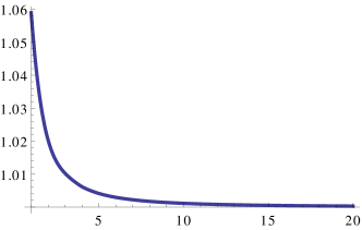
Figure 1: A plot of the ratio $c_{n}^{\infty}/c_{n}$ of the asymptotic form (41) to the numerical results in table 1 for the helicity $\pm 2$ spectral deviation coefficients $c_{n}$.

Figure 1 shows a comparison of this asymptotic form with the numerical results in table 1. For the lowest $n=1$ mode, the deviation from the asymptotic scaling (41) is approximately $6\%$ (far larger than the precision of the results in table 1). But by $n=5$ the asymptotic form is accurate to about half a percent. The rapid approach to the asymptotic form (41) could have been anticipated from the fact that already for modest values of $n$ the coefficients $c_{n}$ become quite large compared to unity. Examination of the rate of convergence confirms the expected $1/n^{2}$ scaling of the deviation.

To summarize, we have shown that helicity $\pm 2$ quasinormal mode frequencies, for large wavenumbers, have the form (16) with $\alpha=4/3$ and $s_{\alpha}^{\infty}$ having phase $-\pi/3$. Continuing the WKB analysis, it is straightforward to show that the next term in the large-$q$ expansion is ${\mathcal{O}}(q^{-1})$. Therefore, for large wavenumbers, helicity $\pm 2$ quasinormal mode frequencies are given by

$$\omega_{n}(q)=q+c_{n}\,e^{-i\pi/3}\,q^{-1/3}+{\mathcal{O}}(q^{-1})\,,$$ (43)

plus reflected frequencies $-\omega_{n}(q)^{*}$, with the real coefficients $\{c_{n}\}$ shown in table 1. These coefficients have the large order asymptotic form (41). Restoring factors of $\pi T$ gives the result (1) quoted in the introduction.

III Quasinormal mode frequencies: numerics

To validate the large-$q$ asymptotics (43) and examine the accuracy of this approximation for intermediate ranges of wavenumber, we use pseudo-spectral methods Boyd (2001) to solve numerically the quasinormal mode equations for a wide range of wavenumbers. This extends previous work in ref. Kovtun and Starinets (2005). We consider first the helicity $\pm 2$ case, and then examine helicity $\pm 1$ and 0.

III.1 Helicity $\pm 2$

As previously noted, frequencies for which the helicity $\pm 2$ quasinormal mode equation (9) has solutions satisfying the required regularity conditions at horizon and boundary come in pairs with opposite real parts (and identical imaginary parts): $\{\omega_{n}\}$ and $\{-\omega_{n}^{*}\}$. So it is sufficient to consider only the positive frequency spectrum, i.e., $\mathop{\rm Re}\omega\geq 0$.

To apply spectral methods, it is convenient to return to the original form (9) of the helicity $\pm 2$ QNM equation. Representing $h$ as a (truncated) series of Chebyshev polynomials,

$$h(u)=\sum_{k=0}^{M}\>f_{k}\>T_{k}(2u{-}1)\,,$$ (44)

automatically satisfies the required regularity conditions at $u=0$ and 1. Demanding that equation (9) [multiplied by $u(1{-}u^{2})$] be satisfied at each point $u=u_{k}$ on the collocation grid,

$$u_{k}\equiv\tfrac{1}{2}\left[1-\cos(k\pi/M)\right],$$ (45)

for $k=0,{\cdots},M$, yields a finite set of linear equations of the form

$$(A-\omega B)\,\vec{f}=0\,,$$ (46)

where, given an explicit choice of the wavevector ${\bf q}$, $A$ and $B$ are numerical $(M{+}1)\times(M{+}1)$ matrices. The generalized eigenvalue problem (46) may be efficiently solved in ${\mathcal{O}}(M^{3})$ time using standard methods. Results for the first fifteen helicity $\pm 2$ quasinormal mode frequencies $\omega_{n}(q)$ [or rather, the deviation ($\omega_{n}(q){-}q$)], for wavevectors $q=10$, 20, 40, 80 and 160, are shown in table 4 of appendix A.

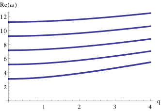
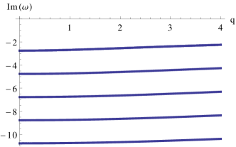
Figure 2: Real (left) and imaginary (right) parts of the first five helicity $\pm 2$ quasinormal frequencies, in units of $\pi T$, for small and intermediate wavevectors, $q\leq 4\pi T$.

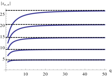
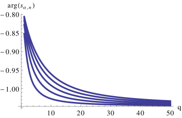
Figure 3: Modulus (left) and phase (right) of the dispersive correction function $s_{\alpha,n}(q)$ for the first five helicity $\pm 2$ quasinormal modes, as a function of wavenumber $q$ (in units of $\pi T$). The complete quasinormal mode frequency is related to $s_{\alpha,n}(q)$ by eq. (47). The horizontal dashed lines show the asymptotic values $c_{n}$ given in table 1. For each mode, one sees that the magnitude of $s_{\alpha,n}(q)$ approaches the asymptotic value $c_{n}$ while the phase approaches $-\pi/3$. Convergence is fastest for the lowest modes.

The real and imaginary parts of the first five helicity $\pm 2$ quasinormal modes are plotted in figure 2 for modest wavenumbers up to $4\pi T$. We have verified that our quasinormal frequencies for $q{=}2$ agree with those given in app. B of ref. Kovtun and Starinets (2005). To present results for larger wavenumbers in a manner which allows easy comparison with the asymptotic form (43), we use the definition (16) of the dispersive correction function (with $\alpha=4/3$), repeated here,

$$\omega_{n}(q)\equiv q+s_{\alpha,n}(q)\,q^{-1/3}\,.$$ (47)

The magnitude and phase of the dispersive correction $s_{\alpha,n}(q)$ for the first 5 modes are shown in figure 3 for wavenumbers up to $q/(\pi T)=50$. One sees, as expected, that $s_{\alpha,n}(q)$ approaches the asymptotic value $c_{n}\,e^{-i\pi/3}$ extracted from the WKB analysis. Lower modes converge faster than higher modes. The rapid rise of the magnitude $|s_{\alpha,n}(q)|$ as $q$ increases from zero is an artifact of definition (47) (since $\omega_{n}(q)$ has a finite $q\to 0$ limit). But the leveling off of the magnitude after this rise provides a clear visual indicator of the onset of the asymptotic regime. From the figure it might appear that the convergence of the magnitude of $s_{\alpha,n}(q)$ toward its asymptotic value $c_{n}$ is considerably faster than the convergence of the phase to $-\pi/3$. This, however, is an illusion produced by the rather compressed range of the ordinate in the right hand plot (which was chosen to make the different phase curves visually distinct).

One may parameterize the raw data in table 4 of appendix A using the functional form

$$\omega_{n}(q)-q=A_{n}^{(1)}\,q^{-1/3}+A_{n}^{(2)}\,q^{-1}+A_{n}^{(3)}\,q^{-5/3}+A_{n}^{(4)}\,q^{-7/3}+A_{n}^{(5)}\,q^{-3},$$ (48)

and demanding that the result reproduce the values in table 4. This form is a truncation of the series which is generated by higher order asymptotic analysis. The resulting values for the first coefficient $A_{n}^{(1)}$, when multiplied by $e^{i\pi/3}$, provide independent estimates of the asymptotic coefficients $\{c_{n}\}$. These estimates, based on what is effectively an extrapolation to $q=\infty$, are less accurate than the values listed in table 1, but the agreement is quite good. The deviation is less than a part in $10^{4}$ for the first few modes, but grows to about half a percent for $n=15$. (This reflects the slower approach to the large-$q$ asymptotic form of progressively higher modes.) Moreover, we have explicitly tested that using the parameterization (48) of the data in table 4, the resulting functions reproduce the directly calculated values of the quasinormal mode frequencies used to produce figure 3 (showing the range $10\leq q\leq 50$) to within a precision of two parts in $10^{4}$.

III.2 Helicity $\pm 1$ and 0

To analyze perturbations with helicity $\pm 1$ and 0, it is convenient to use the gauge invariant linear combinations of metric perturbations introduced by Kovtun and Starinets Kovtun and Starinets (2005). With a Fefferman-Graham form for the metric of the black brane geometry,

$$ds^{2}=\frac{1}{z}\left[-(1{-}z^{2})\,d\tau^{2}+d{\bf x}^{2}\,\right]+\frac{dz^{2}}{4z^{2}(1{-}z^{2})}\,,$$ (49)

helicity $\pm 1$ and 0 linear combinations are, respectively,

$$Z_{1} \equiv z\left(q\,\delta g_{\tau x_{1}}+\omega\,\delta g_{ux_{1}}\right),$$ (50a)

$$Z_{2} \equiv z\left\{\omega^{2}\,\delta g_{x_{3}x_{3}}+2\omega q\,\delta g_{\tau x_{3}}+q^{2}\,\delta g_{\tau\tau}+q^{2}\left[(1{-}z^{2})+2u^{2}-\omega^{2}/q^{2}\right]\left(\delta g_{x_{1}x_{1}}+\delta g_{x_{2}x_{2}}\right)\right\}.$$ (50b)

Decoupled second order linear equations satisfied by these fluctuations were derived in ref. Kovtun and Starinets (2005). Converting to our preferred infalling coordinates leads to the following equations for these perturbations,

$$0 =\widetilde{Z}_{1}^{\prime\prime}+\left[\frac{5}{u}+\frac{2i\omega}{f}-\frac{4u^{3}\omega^{2}}{f\,(\omega^{2}-q^{2}f)}\right]\widetilde{Z}_{1}^{\prime}+\left[\frac{i\omega-uq^{2}}{uf}-4\omega\frac{4u^{3}\omega+i(q^{2}-\omega^{2})}{uf\,(\omega^{2}-q^{2}f)}\right]\widetilde{Z}_{1}\,,$$ (51)

$$0 =\widetilde{Z}_{2}^{\prime\prime}+\left[\frac{1}{u}+\frac{2i\omega}{f}+\frac{4u^{4}(2q^{2}-3\omega^{2})-12(q^{2}{-}\omega^{2})f}{uf\,(3\omega^{2}-(f{+}2)\,q^{2})}\right]\widetilde{Z}_{2}^{\prime}$$

$$\;\;\qquad{}+\left[-\frac{q^{2}}{f}+\frac{16(q^{2}-3\omega^{2})-15i\omega\,(q^{2}{-}\omega^{2})-3iq^{2}\omega u^{4}}{uf\,(3\omega^{2}-(f{+}2)\,q^{2})}\right]\widetilde{Z}_{2}\,,$$ (52)

with $f(u)\equiv 1-u^{4}$. Details of the transformation yielding these equations are given in appendix C. The required boundary conditions for the functions $\widetilde{Z}_{1}(u)$ and $\widetilde{Z}_{2}(u)$ are just regularity at both horizon ($u{=}1$) and boundary ($u{=}0$). Frequencies for which solutions satisfying these boundary conditions exist are either pure imaginary, or else come in pairs with opposite real parts, $\omega$ and $-\omega^{*}$. Therefore, without loss of generality, in the following discussion we consider $\mathop{\rm Re}\omega\geq 0$.

After multiplying the helicity $\pm 1$ equation (51) by its frequency-dependent denominator $\omega^{2}-q^{2}f$, and likewise multiplying the helicity 0 equation (52) by $3\omega^{2}-(f{+}2)\,q^{2}$, both equations become cubic generalized eigenvalue problems of the form

$$\left(\omega^{3}\,O_{3}+\omega^{2}\,O_{2}+\omega\,O_{1}+O_{0}\right)\widetilde{Z}=0\,,$$ (53)

where each $O_{i}$ is a linear operator. By replicating the function space on which one works, this may be converted into a conventional generalized eigenvalue problem, $A\,X=\omega\,B\,X$, where $X\equiv(\omega^{2}\widetilde{Z},\omega\widetilde{Z},\widetilde{Z})$ and

$$A\equiv\begin{pmatrix}O_{2}&O_{1}&O_{0}\\ -\mathds{1}&0&0\\ 0&-\mathds{1}&0\end{pmatrix}\,,\qquad B\equiv\begin{pmatrix}-O_{3}&~{}0~{}&~{}0~{}\\ 0&\mathds{1}&0\\ 0&0&\mathds{1}\end{pmatrix}\,.$$ (54)

Applying pseudo-spectral methods to convert the linear radial differential operators $O_{i}$ into matrices and solving the resulting finite dimensional generalized eigenvalue problem proceeds in the same manner described previously. Results for the first fifteen helicity $\pm 1$ and 0 quasinormal mode frequencies $\omega_{n}(q)$ [or rather, the deviation ($\omega_{n}(q){-}q$)], for wavevectors $q=10$, 20, 40, 80 and 160, are given in tables 5 and 6 of appendix A.

We first discuss helicity $\pm 1$ perturbations. The real and imaginary parts of the first five quasinormal frequencies are plotted in fig. 4 for $q\leq 4\pi T$. For modest wavenumbers, $q\lesssim 2.6\,\pi T$, the most weakly damped mode is a hydrodynamic shear mode whose frequency is pure imaginary and vanishes as $q\to 0$. This frequency, which is shown by dashed lines in fig. 4, moves down the imaginary axis as $q$ increases. As seen in the figure and noted in ref. Amado et al. (2008), the frequency of this mode crosses the imaginary parts of other mode frequencies (having non-zero real parts) at various intermediate values of $q$. For $q\gg T$, this mode becomes highly damped and is not among the minimally damped modes discussed below.

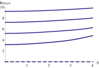
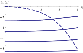
Figure 4: Real (left) and imaginary (right) parts of the first five helicity $\pm 1$ quasinormal mode frequencies in units of $\pi T$, for small and intermediate wavevectors, $q\leq 4\pi T$. There is one diffusive mode with pure imaginary frequency which approaches zero as $q\to 0$. The frequency of this hydrodynamic shear mode is shown with a dashed curve in both plots.

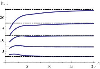
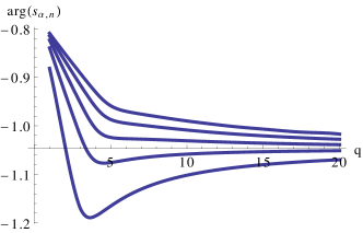
Figure 5: Modulus (left) and phase (right) of the dispersive correction $s_{\alpha,n}(q)$ for the first five (non-hydrodynamic) helicity $\pm 1$ quasinormal modes, as a function of wavenumber $q$ (in units of $\pi T$). The complete quasinormal mode frequency is related to $s_{\alpha,n}(q)$ by eq. (47). For each mode, one sees that the magnitude $|s_{\alpha,n}(q)|$ becomes approximately constant as $q$ increases, and the corresponding phase approaches a value close to $-\pi/3$. Horizontal dashed lines show the asymptotic values extracted using the parameterization (48) applied to the data in table 5, and listed in table 2. Near-asymptotic behavior sets in for moderate values of wavevector, $q/(\pi T)\approx 5$.

To examine larger values of $q$ and the approach to the asymptotic regime, we plot in fig. 5 the magnitude and phase of the dispersive correction $s_{\alpha,n}(q)$, defined via eq. (47), of the lowest five helicity $\pm 1$ modes (excluding the hydrodynamic shear mode) for $q/(\pi T)$ up to 20. Unlike the helicity $\pm 2$ case, one sees non-monotonic behavior in the lowest modes as $q$ increases. Although we have not done an independent WKB calculation for helicity $\pm 1$ to determine asymptotic values directly, from the plots it certainly appears that the magnitudes $|s_{\alpha,n}(q)|$ are approaching constant values while all phases are converging to a value near $-\pi/3$. Near-asymptotic behavior begins to be apparent for quite modest values of wavenumber, $q/(\pi T)\approx 5$.

helicity $\pm 1$ modes
$n$	$|c_{n}|$	$\arg(c_{n})$	$n$	$|c_{n}|$	$\arg(c_{n})$	$n$	$|c_{n}|$	$\arg(c_{n})$
1	$2.69717$	$0.000001$	6	$30.0107$	$0.00051$	11	$67.2833$	$0.00283$
2	$6.90578$	$0.000003$	7	$36.8644$	$0.00087$	12	$75.5084$	$0.00325$
3	$11.8887$	$0.000022$	8	$44.0488$	$0.00133$	13	$83.9421$	$0.00354$
4	$17.4637$	$0.000093$	9	$51.5313$	$0.00183$	14	$92.5695$	$0.00369$
5	$23.5271$	$0.000248$	10	$59.2841$	$0.00235$	15	$101.379$	$0.00366$

Table 2: Estimates for the magnitude and phase of the asymptotic spectral deviation coefficients $\{c_{n}\}$ for the first fifteen helicity $\pm 1$ quasinormal mode frequencies, extracted from the parameterization (48) of the helicity $\pm 1$ data in table 5 of appendix A. Within the accuracy of the parameterization, the phases of $c_{n}$ are all compatible with zero.

One may parameterize the helicity $\pm 1$ data in table 5 of appendix A using the same functional form (48) suggested by the helicity $\pm 2$ WKB analysis. The resulting parameterizations reproduce the directly calculated values of quasinormal mode frequencies used to produce figure 5 (showing the range $10\leq q\leq 20$) to within a precision of five parts in $10^{4}$. Although not a formal proof, the consistency and accuracy of the parameterization (48), when applied to our helicity $\pm 1$ data, strongly suggests that helicity $\pm 1$ quasinormal mode frequencies have the same large-$q$ asymptotic form (43) as do helicity $\pm 2$ modes. The first coefficients $\{A_{n}^{(1)}\}$ of the parameterization, when multiplied by $e^{i\pi/3}$, directly give estimates of the asymptotic spectral deviation coefficients $\{c_{n}\}$ for helicity $\pm 1$ modes. Table 2 lists these estimates for the first fifteen modes. Within the accuracy of the parameterization (as determined by our tests with $10<q<20$), the phases of the asymptotic coefficients $c_{n}$ are all compatible with zero.

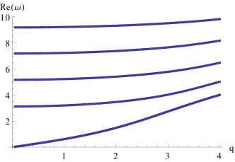
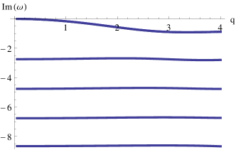
Figure 6: Real (left) and imaginary (right) parts of the first five helicity 0 quasinormal frequencies in units of $\pi T$, for small and intermediate wavevectors, $q\leq 4\pi T$. There is one hydrodynamic (sound) mode whose frequency vanishes as $q\to 0$.

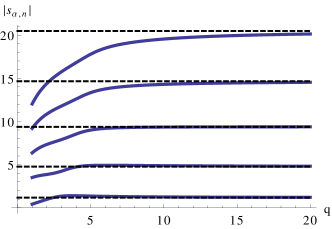
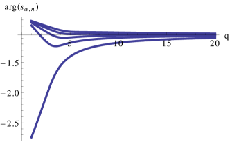
Figure 7: Modulus (left) and phase (right) of the dispersive correction $s_{\alpha,n}(q)$ for the first five helicity 0 quasinormal modes, as a function of wavevector $q$ (in units of $\pi T$). The complete quasinormal mode frequency is related to $s_{\alpha,n}(q)$ by eq. (47). Once again, for each mode one sees that the magnitude $|s_{\alpha,n}(q)|$ becomes approximately constant as $q$ increases, and the corresponding phase approaches a value close to $-\pi/3$. Horizontal dashed lines show the asymptotic values extracted using the parameterization (48) applied to the data in table 6, and listed in table 3. Near-asymptotic behavior sets in for $q/(\pi T)\approx 5$.

We now turn to helicity 0 modes, whose behavior largely parallels that of the helicity $\pm 1$ modes just discussed. Fig. 6 plots the real and imaginary parts of the first five helicity 0 quasinormal modes for $q/(\pi T)\leq 4$. There is one hydrodynamic helicity 0 (sound) mode, whose frequency vanishes as $q\to 0$ (with $\mathop{\rm Re}\omega={\mathcal{O}}(q)$ and $\mathop{\rm Im}\omega={\mathcal{O}}(q^{2})$). As noted in ref. Chesler et al. (2012), the helicity 0 hydrodynamic sound mode smoothly evolves from small to large values of $q$ and always remains the most weakly damped mode. Its damping, as measured by $\mathop{\rm Im}\omega/\mathop{\rm Re}\omega$, rises linearly from $q=0$, reaches a maximum at $q/(\pi T)\approx 2.120$, and then decreases as ${\mathcal{O}}(q^{-4/3})$ as $q$ continues to grow. Fig. 7 plots the modulus and phase of the spectral deviation function $s_{\alpha,n}(q)$ for these modes out to $q/(\pi T)=20$. From the figure one sees, once again, that the magnitudes $|s_{\alpha,n}(q)|$ are nearly constant for $q/(\pi T)\gtrsim 5$ and all phases approach a value close to $-\pi/3$.

As before, one may parameterize the helicity 0 data in table 6 of appendix A with the functional form (48) used earlier. The resulting parameterizations reproduce directly calculated values of helicity 0 quasinormal mode frequencies for wavevectors throughout the range $10\leq q\leq 20$ to within a precision of a part in $10^{4}$. This consistency strongly suggests that helicity 0 quasinormal mode frequencies also have the same asymptotic form (43). Table 3 shows our resulting estimates, extracted from this simple parameterization, for the spectral deviation coefficients $\{c_{n}\}$ for the first fifteen helicity 0 modes. Within the accuracy of the parameterization, the phases of the asymptotic coefficients $c_{n}$ are, once again, all compatible with zero.

helicity $0$ modes
$n$	$|c_{n}|$	$\arg(c_{n})$	$n$	$|c_{n}|$	$\arg(c_{n})$	$n$	$|c_{n}|$	$\arg(c_{n})$
1	$1.17236$	$0.000003$	6	$26.7489$	$0.000363$	11	$63.2685$	$0.002594$
2	$4.76469$	$0.000003$	7	$33.4190$	$0.000675$	12	$71.3809$	$0.003046$
3	$9.36737$	$0.000010$	8	$40.4393$	$0.001086$	13	$79.7103$	$0.003402$
4	$14.6512$	$0.000050$	9	$47.7737$	$0.001570$	14	$88.2406$	$0.003624$
5	$20.4734$	$0.000158$	10	$55.3920$	$0.002087$	15	$96.9584$	$0.003684$

Table 3: Estimates for the magnitude and phase of the asymptotic spectral deviation coefficients $\{c_{n}\}$ for the first fifteen helicity $0$ quasinormal mode frequencies, extracted from the parameterization (48) of the helicity $0$ data in table 6 of appendix A. Within the accuracy of the parameterization, the phases of $c_{n}$ are all compatible with zero.

In summary, we have compelling evidence that, for all helicities of metric perturbations, quasinormal mode frequencies have the large $q$ asymptotic form $\omega_{n}(q)=q+c_{n}\,e^{-i\pi/3}\,q^{-1/3}+{\mathcal{O}}(q^{-1})$, with ${\mathcal{O}}(q^{-4/3})$ relative corrections to a massless $\omega=\pm q$ dispersion relation, and with real positive coefficients $\{c_{n}\}$ characterizing the dispersive correction. This large-$q$ asymptotic form is reasonably accurate, at least for low order modes, down to $q/(\pi T)\approx 5$.

III.3 Large order asymptotics

Comparing the helicity $\pm 2$ spectral deviation coefficients listed in table 1 with our corresponding helicity $\pm 1$ or 0 values shown in tables 2 and 3, it is clear by inspection that the helicity $\pm 1$ and 0 spectral deviation coefficients grow about as fast with increasing mode number as do the helicity $\pm 2$ coefficients. Given the known asymptotic behavior (41) of the helicity $\pm 2$ coefficients, it is natural to try fitting our estimates of helicity $\pm 1$ and 0 spectral deviation coefficients using a function of the form $b\,(2n+a)^{4/3}$. It is also instructive, for comparison, to apply the same procedure to estimates of the helicity $\pm 2$ spectral deviation coefficients generated by the parameterization (48) applied to the data of table 4. In performing these fits, we set to zero the small residual phases in the $c_{n}$ estimates (which are all compatible to zero, within the accuracy of the parameterizations).

For all helicities, the resulting best fit value of the overall coefficient $b$ coincides with the analytically known value (42) of the helicity $\pm 2$ coefficient $K=\tfrac{1}{2}\left[\sqrt{\pi}\,\Gamma(\tfrac{7}{4})/\Gamma(\tfrac{5}{4})\right]^{4/3}=1.092\cdots$ to within a percent, and is quite insensitive to whether one fits all 15 modes or, for example, just modes 6 to 10. We take this as compelling evidence that our fitting function correctly describes the large order asymptotic behavior of spectral deviation coefficients for helicities $\pm 1$ and 0, as well as $\pm 2$, with the same overall coefficient $K$ for all helicities.

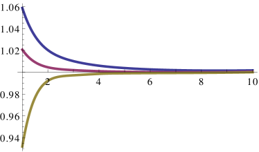
Figure 8: Plots of the ratio $c_{n}^{\infty}/c_{n}$ of the large order asymptotic form (55) of the spectral deviation coefficients to the values (for the first ten modes) obtained from applying the parameterization (48) to the data of appendix A. From top to bottom the curves correspond to helicity $\pm 2$, $\pm 1$, and $0$. The asymptotic form is $c_{n}^{\infty}=K(2n+|s|-1)^{4/3}$ for helicity $s$.

If one fixes the overall coefficient $b=K$, then the resulting best fit value for the shift $a$ is very close to an integer, and is reasonably insensitive to the limits of the fitting range. For helicity $\pm 2$ the best fit value for the shift $a$ equals the correct answer $+1$ to within four percent. For helicity $\pm 1$, the best fit value for the shift $a$ is quite close to zero, somewhere in the interval $-0.002$ to $-0.03$ depending on the chosen limits of the fitting range. And for helicity 0, the best fit value for the shift $a$ equals $-1$ to within a percent or two. Given that we are only fitting data up to $n=15$, these results are nicely consistent with the known large order asymptotic form (41) for the helicity $\pm 2$ spectral deviation coefficients, and very clearly suggest corresponding large order asymptotic forms for helicity $\pm 1$ and 0 coefficients, as reported in the introduction. Explicitly, for helicity $s$, $c_{n}\sim c_{n}^{\infty}\,[1+{\mathcal{O}}(n^{-2})]$ with

$$c_{n}^{\infty} \equiv K\,(2n+|s|-1)^{4/3}\,.$$ (55)

Figure 8 shows, for each helicity, a comparison of this asymptotic form with our numerical estimates for spectral deviation coefficients produced by using the functional form (48) to parameterize the data of tables 4, 5 and 6 of appendix A. The uppermost curve shows helicity $\pm 2$, the middle curve is helicity $\pm 1$, and the lower curve shows helicity 0. Fast approach to the large order asymptotic form (55) is manifest. The helicity $\pm 2$ curve shown here agrees with the plot in fig. 8, which used the the highly accurate $c_{n}$ values of table 1, up to a permille. Curiously, the approach to the asymptotic form is even faster for helicity $\pm 1$ and 0 compared to helicity $\pm 2$. For helicity $\pm 1$, the deviation is only 2% for the lowest $n=1$ mode, and falls to half a percent or less for all higher modes. For helicity 0, the deviation is $-7$% for the lowest mode, but also falls to half a percent or less for all higher modes.

IV Planar shocks propagating in $\mathcal{N}\,{=}\,4$ SYM plasma

The general solution for the time evolution of linearized perturbations to the metric of the AdS black brane geometry (with fixed boundary geometry and incoming conditions at the horizon), may be represented as a linear combination of quasinormal modes,

$$\delta g(t,{\bf x},u)=\sum_{n}\int\frac{d^{3}q}{(2\pi)^{3}}\>e^{-i\omega_{n}(q)t+i{\bf q}\cdot{\bf x}}\,A_{n}({\bf q})\,u^{2}\,h_{n}(u;q)\,H_{n}\,,$$ (56)

where $q\equiv|{\bf q}|$. The sum runs over all quasinormal modes (of metric perturbations) with the symmetries of interest, $A_{n}({\bf q})$ is the amplitude of a given mode, and $H_{n}$ encodes the tensor structure of the mode, e.g., $H_{n}=dx_{1}\otimes dx_{2}+dx_{2}\otimes dx_{1}$ for helicity $\pm 2$ modes with the indicated polarization. Extracting a factor of $u^{2}$, as shown, allows one to fix the normalization of the radial profiles $h_{n}(u;q)$ by requiring that they have a fixed boundary value, $h_{n}(0;q)=1$.

The corresponding change in the expectation value of the energy-momentum tensor of the dual QFT is then de Haro et al. (2001)

$$\langle\delta T_{\mu\nu}(t,{\bf x})\rangle =\kappa\sum_{n}\int\frac{d^{3}q}{(2\pi)^{3}}\>e^{-i\omega_{n}(q)t+i{\bf q}\cdot{\bf x}}A_{n}({\bf q})\,H_{n,\mu\nu}\,,$$ (57)

where $\kappa=m^{4}L^{3}/(4\pi G)$ with $L$ the AdS curvature scale which, elsewhere, has been set to unity. In terms of field theory quantities, $\kappa=\tfrac{1}{2}N_{c}^{2}\pi^{2}T^{4}$, where $N_{c}$ is the rank of the SU($N_{c}$) gauge group of $\mathcal{N}\,{=}\,4$ SYM.

Similarly, if one considers a perturbation to the equilibrium state created by a time dependent source coupled to the QFT stress-energy tensor (i.e., a fluctuation in the spacetime geometry of the 4D field theory), then the induced response is given by a convolution with the retarded stress-energy correlator,

$$\langle\delta T_{\mu\nu}(t,{\bf x})\rangle=\int\frac{d\omega\,d^{3}q}{(2\pi)^{4}}\>e^{-i\omega t+i{\bf q}\cdot{\bf x}}\,G_{\mathrm{R}}(\omega,{\bf q})_{\mu\nu}^{\hphantom{\mu\nu}\rho\sigma}\>j(\omega,{\bf q})_{\rho\sigma}\,.$$ (58)

Quasinormal mode frequencies correspond to the poles of the retarded Green’s function Son and Starinets (2002), so evaluating the frequency integral using Cauchy’s theorem yields

$$\langle\delta T_{\mu\nu}(t,{\bf x})\rangle=\sum_{n}\int\frac{d^{3}q}{(2\pi)^{3}}\>e^{-i\omega_{n}(q)t+i{\bf q}\cdot{\bf x}}\,R_{n}({\bf q})^{\hphantom{\mu\nu}\rho\sigma}_{\mu\nu}\>j(\omega_{n}(q),{\bf q})_{\rho\sigma}\,,$$ (59)

where $R_{n}({\bf q})$ denotes the residue of the retarded Green’s function $G_{\mathrm{R}}(\omega,{\bf q})$ at $\omega_{n}(q)$.

Both expressions (57) and (59) represent the response as a sum of contributions from quasinormal modes, and make it obvious that at sufficiently late times the response will be dominated by those modes whose frequencies $\omega_{n}({\bf q})$ have the smallest (in magnitude) negative imaginary parts. Specifically, these are long wavelength hydrodynamic modes with $q\ll T$, together with the short wavelength modes with $q\gg T$ discussed above. To examine qualitative features of the resulting evolution, it will be sufficient to use the asymptotic form (43) of quasinormal mode frequencies, repeated here for convenience,

$$\omega_{n}(q)=\pm\left[q+\tfrac{1}{2}c_{n}\,(\pi T)^{4/3}\,q^{-1/3}\right]-i\tfrac{\sqrt{3}}{2}\,c_{n}\,(\pi T)^{4/3}\,q^{-1/3}+{\mathcal{O}}\big{(}T^{3}q^{-2}\big{)}\,,$$ (60)

which for low order modes, as discussed in sec. III, is already quite accurate at intermediate values of $q/T$. (Explicit values of the coefficients $c_{n}$ are given in tables 1, 2 and 3.)

IV.1 Fine structures outlive coarse

Consider a metric perturbation $\delta g$, represented in the form (56), which at time $t=0$ has rapid spatial variation and a spatial Fourier transform concentrated near some wavevector ${\bf q}_{0}$ with $|{\bf q}_{0}|\gg T$. The asymptotic form (60) implies that the characteristic relaxation time of such an excitation will be of order $\tau(q_{0})\equiv q_{0}^{1/3}(\pi T)^{-4/3}$, with higher modes (larger $n$) damping faster than lower modes. At times comparable or larger than this relaxation time, dominant contributions will come from the $n{=}1$ mode with wavenumbers near ${\bf q}_{0}$. Provided the perturbation is sufficiently small, so a linearized treatment is valid, there is no mode-mixing populating other ranges of wavevector. The resulting late-time energy-momentum tensor (57) is then well described by just the $n\,{=}\,1$ contribution,

$$\langle\delta T_{\mu\nu}\rangle=\kappa\int\frac{d^{3}q}{(2\pi)^{3}}\>e^{i\phi({\bf q})}\,\widetilde{A}({\bf q})\,H_{1,\mu\nu}\,,$$ (61)

with a damped amplitude

$$\widetilde{A}({\bf q})\equiv A_{1}({\bf q})\,\exp\big{[}{-t\,\tfrac{\sqrt{3}}{2}\,c_{1}\,(\pi T)^{4/3}\,q^{-1/3}}\big{]}\,,$$ (62)

and rapidly varying phase

$$\phi({\bf q})\equiv{\bf q}\cdot{\bf x}-\big{[}q+\tfrac{1}{2}\,c_{1}\,(\pi T)^{4/3}\,q^{-1/3}\big{]}\,t\,.$$ (63)

If one asks when a disturbance, initially localized near ${\bf x}=0$ at time 0, will reach a distant point ${\bf x}$, the dominant contributions to the integral (61) come from the neighborhood of the stationary phase point where $\nabla\phi({\bf q})=0$. (provided $\widetilde{A}({\bf q})$ is slowly varying on the scale of $|{\bf x}|^{-1}$). This yields the standard result that disturbances localized in wavenumber near ${\bf q}={\bf q}_{0}$ travel at the group velocity,

$${\bf v}_{\rm g}({\bf q}_{0})\equiv\nabla\mathop{\rm Re}(\omega({\bf q}_{0}))=v_{\rm g}(q_{0})\,\hat{\bf q}_{0}\,,\qquad v_{\rm g}(q_{0})\sim 1-\tfrac{1}{6}\,c_{1}\,(\pi T/q_{0})^{4/3}\,,$$ (64)

and hence arrive at position ${\bf x}=d\,\hat{\bf q}_{0}$ at time $t=d/v_{\rm g}(q_{0})$.

The damping (62) decreases monotonically with increasing wavenumber, while the group velocity (64) increases monotonically, asymptotically approaching the speed of light. Hence, shorter wavelength features attenuate slower, and propagate faster, than longer wavelength features. For disturbances with a significant range of wavenumbers, the overall evolution will reflect a combination of the wavenumber dependent damping (62) and the dispersive propagation (64).

IV.2 Planar shocks at late times

The evolution of planar shocks in a strongly coupled $\mathcal{N}\,{=}\,4$ SYM plasma provides an interesting, concrete illustration of the above features. At zero temperature, planar shocks (composed of helicity 0 perturbations) move at the speed of light with no dispersion or damping. For a shock propagating in, say, the $+\hat{x}_{3}$ direction with an arbitrary longitudinal energy density profile $\kappa\,h(x_{3})$, stress-energy components at time $t$ are

$$\delta T^{00}(t,{\bf x})=\delta T^{03}(t,{\bf x})=\delta T^{33}(t,{\bf x})=\kappa\,h(x_{3}{-}t)\,,$$ (65)

with all other components vanishing. Equivalently,

$$\langle\delta T_{\mu\nu}\rangle=\kappa\int\frac{dq_{3}}{2\pi}\>e^{iq_{3}(x_{3}-t)}\,A(q_{3})\>(dx_{3}{-}dt)_{\mu}\,(dx_{3}{-}dt)_{\nu}\,,$$ (66)

with $A(q_{3})$ the Fourier transform of $h(x_{3})$. The dual geometry is an exact analytic solution of Einstein’s equations Chesler and Yaffe (2011). Analogous planar stress-energy perturbations with helicity $\pm 1$ or $\pm 2$ tensor structures correspond to solutions of Einstein’s equations linearized about $AdS_{5}$, but analytic solutions at the non-linear level are not known.

We are interested in the modification in the evolution of planar shocks induced by the presence of a background thermal plasma. We assume that the amplitude of the shock is sufficiently small so that a linearized treatment is adequate. And, for simplicity, we assume that the perturbation has a single tensor structure corresponding to either helicity 0, $\pm 1$, or $\pm 2$.

Planarity of the shock implies that the expression (57) for the stress-energy (at times $t\geq 0$) simplifies to a one-dimensional Fourier transform,

$$\langle\delta T_{\mu\nu}(t,x_{3})\rangle=\kappa\sum_{n}\int\frac{dq_{3}}{2\pi}\>e^{-i\omega_{n}(q_{3})t+iq_{3}x_{3}}\,A_{n}(q_{3})\,H_{\mu\nu}\,,$$ (67)

with the coefficients $\{A_{n}(q_{3})\}$ characterizing the chosen shock profile at time $t=0$.

As discussed in the previous subsection, since large-$q$ modes experience minimal damping, rapidly varying features in the longitudinal profile of the shock will outlive more slowly varying features. A particularly clear picture emerges for narrow shocks. A shock with narrow width $w\ll 1/T$ will have a broad Fourier spectrum extending from small wavenumbers at least up to $|q_{3}|\sim 1/w$. More precisely, the breadth of the Fourier spectrum reflects the (inverse) scale of variation of the sharpest spatial features. As a coherent superposition of many different wavevectors, small differences in the propagation of different wavenumbers will imprint themselves on the evolution of the shock profile. In particular, since the speed of propagation approaches the speed of light as $|q_{3}|\to\infty$, contributions from the highest-wavenumber modes will accumulate very near the light cone, forming an increasingly sharp leading edge. These sharp features will persist longer than contributions from lower wavenumbers (except for very small $q$ hydrodynamic modes) which attenuate more quickly.

To illustrate this explicitly with simple examples, we consider perturbations which are dominated by the lowest quasinormal mode (of a given helicity), so that

$$\langle\delta T_{\mu\nu}(t,x_{3})\rangle=\kappa\int\frac{dq_{3}}{2\pi}\>e^{-i\omega_{1}(q_{3})t+iq_{3}x_{3}}\,A_{1}(q_{3})\,H_{\mu\nu}\,.$$ (68)

One may either regard this as fine-tuning the initial data, or the result of starting with a more general perturbation and waiting to sufficiently late times where higher modes are small compared to the lowest mode. For simplicity, we include only modes with $\mathop{\rm Re}(q_{3}\,\omega_{1}(q_{3}))>0$ in the perturbation (68), with no corresponding contributions from the reflected modes with frequency $-\omega_{1}(q_{3})^{*}$; this means that we are focusing on right-moving perturbations. We compare three different longitudinal profiles,

$$A_{1}^{\rm Gauss}(q)=e^{-\frac{1}{2}\sigma^{2}q^{2}}\,,\qquad A_{1}^{\rm Blob}(q)=\frac{2J_{1}(\sigma q)}{\sigma q}\,,\qquad A_{1}^{\rm Step}(q)=\frac{\sin(\sigma q)}{\sigma q}\,.$$ (69)

These are Fourier transforms of position space profiles $h(x_{3})=\int dq/(2\pi)\>e^{iqx_{3}}\,A_{1}(q)$ which are, respectively, a Gaussian, a semicircular “blob,” and a “top-hat” step function, each normalized to unit area:

$$h^{\rm Gauss}(x_{3})=\frac{e^{-\frac{1}{2}{x_{3}^{2}}/\sigma^{2}}}{\sqrt{2\pi}\,\sigma}\,,\quad h^{\rm Blob}(x_{3})=\frac{2\sqrt{\sigma^{2}{-}x_{3}^{2}}}{\pi\sigma^{2}}\,\Theta(\sigma^{2}{-}x_{3}^{2})\,,\quad h^{\rm Step}(x_{3})=\frac{\Theta(\sigma^{2}{-}x_{3}^{2})}{2\sigma}\,.$$ (70)

We choose $\sigma=1/10$ for $h^{\rm Gauss}$, and $\sigma=1/5$ for $h^{\rm Blob}$ and $h^{\rm Step}$.

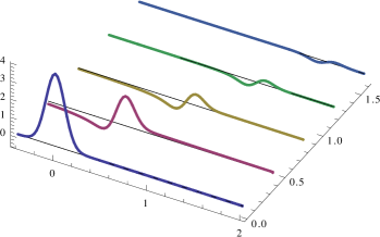
Figure 9: Time evolution of helicity $\pm 2$ perturbations [left] and helicity 0 perturbations [right] for each of the three initial profiles (70): Gaussian, “Blob,” and “Step” [top to bottom]. Snapshots are taken at times $t=0,\frac{1}{2},1,\frac{3}{2},2$ for helicity $\pm 2$, and at $t=0,1,2,3,4,5$ for helicity 0; the different time scales reflect the faster damping of helicity $\pm 2$ perturbations. For the helicity-$2$ perturbations one sees that the longest surviving features are associated with the steepest portions of the initial profile. This is especially apparent with the compactly-supported “blob” and “step” profiles. For helicity $0$ there is, in addition, a visible slowly varying contribution from the hydrodynamic sound mode.

For the dispersion relation $\omega_{1}(q)$ we construct a cubic spline interpolating function from the numerical results of sec. III for low and intermediate wavenumbers, which smoothly connects to the large-$q$ asymptotics of eq. (60). Since the large-$q$ asymptotic form is already quite accurate for intermediate values of $q$, this procedure is straightforward. Figure 9 shows plots of the resulting time evolution for perturbations with each of the above profiles, for the helicity $\pm 2$ tensor structure $dx_{1}\otimes dx_{2}$ as well as the helicity 0 structure $(dx_{3}{-}dt)\otimes(dx_{3}{-}dt)$. Comparing the plots, one clearly sees the stronger damping of helicity $\pm 2$ fluctuations relative to helicity $0$, due to the larger values of the dispersive coefficient $c_{1}$ (cf. tables 1 and 3). For the helicity $\pm 2$ perturbations, shown on the left side of the figure, the longest surviving features are associated with the steepest portions of the initial profile. This is especially apparent for the “blob” and “step” profiles which have compact support. At late times, one sees upward “spikes” which evolve from the portion of the initial profile with large negative gradient, and downward spikes evolving from the steeply rising part of the initial profile.

The helicity 0 evolution, shown on the right-hand side of the figure, shows similar sharp high-$q$ features but with the addition of a slowly varying hydrodynamic (sound) contribution which moves slower than the leading features and gradually broadens. (The speed of sound in the conformal $\mathcal{N}\,{=}\,4$ plasma is $1/\sqrt{3}$ Kovtun and Starinets (2005).) Hence, as time increases there is an increasingly clear separation between the attenuating high-$q$ and low-$q$ remnants.

The helicity 0 planar shocks have a conserved energy (and linear momentum). At late times, the energy and momentum of the shock is entirely carried by the $q\to 0$ hydrodynamic contribution; for the profiles of fig. 9, the upward and downward high-$q$ spikes cancel each other upon integration. More generally, the long-lived fine structure carries little net energy or momentum. This might seem odd, since high momentum quasiparticles (or short wavelength waves) in other contexts can transport energy and momentum. But stress-energy quasinormal modes in strongly coupled (and large $N_{\rm c}$) SYM plasma are perturbations in which the energy density, momentum density, and/or stress of the fluid vary sinusoidally (for non-zero ${\bf q}$) and hence unavoidably vanish upon integration. This is fundamentally different from, say, an electromagnetic wave in vacuum in which the EM field varies sinusoidally but the energy density is quadratic in the wave amplitude and always positive.

V Discussion

We have extended and clarified previous work on quasinormal mode frequencies for metric perturbations of AdS-Schwarzschild black branes, or equivalently stress-energy perturbations in strongly coupled $\mathcal{N}\,{=}\,4$ SYM plasma. The large wavenumber asymptotic behavior has the universal form (60), in all helicity channels, with mode-dependent spectral deviation coefficients shown in tables 1, 2 and 3. The relaxation rate of short wavelength quasinormal modes vanishes asymptotically as $T^{4/3}q^{-1/3}$. We find that the large-$q$ asymptotic form (60) of quasinormal mode frequencies agrees well with the exact values (for low order modes) already at rather moderate values of $q/T$, and thus provides a good approximation over a wide range of scales. The spectral deviation coefficients of high order modes approach the asymptotic form (55) but the coefficients of low order modes deviate from this simple expression.

In the strongly coupled SYM plasma it is noteworthy that hydrodynamic fluctuations are not the only arbitrarily long-lived excitations. The asymptotic vanishing of relaxation rates implies that there are two types of long-lived propagating excitations: long-wavelength sound waves, moving at $v_{\rm s}=c/\sqrt{3}$, and short-wavelength fluctuations with group velocities asymptotically approaching $c$. As vividly seen in figure 9, illustrating examples of planar shock propagation, the decreasing attenuation plus increasing group velocity (as the wavevector $q$ increases) combine to produce sharp, long-lived “spikes” which evolve from the most rapidly varying parts of an initial waveform. This same phenomena is evident in the study Chesler et al. (2012) by Chesler, Ho and Rajagopal of the “cyclotron radiation” produced by circular stirring of an SYM plasma (see fig. 3 of ref. Chesler et al. (2012)). Whether such long-lived “fine structure” could have observable phenomenological consequences in heavy ion collisions is an interesting open question.

There has been considerable discussion in the literature Steineder et al. (2013b); Balasubramanian et al. (2011a, b); Galante and Schvellinger (2012); Steineder et al. (2013a); Stricker (2014, 2013) regarding “top-down” thermalization in strongly coupled SYM, as compared with “bottom-up” thermalization at weak coupling Baier et al. (2001). Evidence suggesting a top-down picture of thermalization at strong coupling comes from the decreasing relaxation times of quasinormal modes as the mode number increases at fixed wavenumber, and related observables probing similar physics. However, interpreting this as top-down thermalization is, in our view, conflating the dephasing or decoherence of highly virtual off-shell excitations ($|\omega|^{2}\gg q^{2})$, with relaxation of high momentum but near on-shell excitations ($|\omega-q|^{2}\ll q^{2}$). It is these latter excitations, corresponding to large wavenumber but low order quasinormal modes, which should be considered when discussing top-down versus bottom-up thermalization. And these hard but low virtuality excitations thermalize slowly at both weak and strong coupling.

Finally, we limited our attention to metric (or stress-energy) perturbations. We expect quasinormal mode frequencies for perturbations in other supergravity fields to have the same universal asymptotic form (60), but it would be worthwhile to demonstrate (or disprove) this explicitly, especially for fermionic fluctuations. We leave such questions for future work.

Appendix A Tabulated results

helicity $\pm 2$
$n$	$q=10$	$q=20$	$q=40$	$q=80$	$q=160$
1	$1.05863-1.75039\,i$	$0.82995-1.41031\,i$	$0.65513-1.12603\,i$	$0.51880-0.89583\,i$	$0.41139-0.71168\,i$
2	$2.20415-3.49828\,i$	$1.71646-2.86252\,i$	$1.34867-2.29987\,i$	$1.06566-1.83424\,i$	$0.84425-1.45862\,i$
3	$3.52349-5.37997\,i$	$2.73704-4.47509\,i$	$2.14189-3.62096\,i$	$1.68857-2.89602\,i$	$1.33636-2.30553\,i$
4	$4.97581-7.33629\,i$	$3.87015-6.20226\,i$	$3.01901-5.05684\,i$	$2.37469-4.05696\,i$	$1.87734-3.23373\,i$
5	$6.52930-9.33352\,i$	$5.09962-8.01283\,i$	$3.96941-6.58524\,i$	$3.11555-5.30074\,i$	$2.46028-4.23071\,i$
6	$8.15996-11.3527\,i$	$6.41236-9.88471\,i$	$4.98539-8.18992\,i$	$3.90521-6.61561\,i$	$3.08037-5.28757\,i$
7	$9.85002-13.3833\,i$	$7.79737-11.8019\,i$	$6.06096-9.85842\,i$	$4.73923-7.99264\,i$	$3.73400-6.39761\,i$
8	$11.5864-15.4192\,i$	$9.24519-13.7526\,i$	$7.19119-11.5808\,i$	$5.61417-9.42475\,i$	$4.41841-7.55557\,i$
9	$13.3592-17.4572\,i$	$10.7476-15.7280\,i$	$8.37186-13.3490\,i$	$6.52726-10.9061\,i$	$5.13137-8.75720\,i$
10	$15.1614-19.4954\,i$	$12.2977-17.7217\,i$	$9.59927-15.1564\,i$	$7.47616-12.4320\,i$	$5.87107-9.99894\,i$
11	$16.9874-21.5328\,i$	$13.8892-19.7288\,i$	$10.8701-16.9972\,i$	$8.45891-13.9981\,i$	$6.63596-11.2778\,i$
12	$18.8329-23.5687\,i$	$15.5171-21.7457\,i$	$12.1812-18.8667\,i$	$9.47378-15.6008\,i$	$7.42475-12.5912\,i$
13	$20.6946-25.6031\,i$	$17.1769-23.7697\,i$	$13.5299-20.7609\,i$	$10.5193-17.2372\,i$	$8.23632-13.9368\,i$
14	$22.5701-27.6357\,i$	$18.8647-25.7988\,i$	$14.9136-22.6763\,i$	$11.5940-18.9042\,i$	$9.06968-15.3127\,i$
15	$24.4571-29.6665\,i$	$20.5772-27.8314\,i$	$16.3299-24.6099\,i$	$12.6966-20.5994\,i$	$9.92396-16.7170\,i$

Table 4: Dispersive corrections $\omega_{n}(q)-q$ of the first fifteen helicity $\pm 2$ quasinormal mode frequencies, for wavenumbers $q=10$, 20, 40, 80 and 160. Both frequencies and wavenumbers are in units of $\pi T$. Values were obtained by numerically solving eqn. (9); all digits shown are accurate.

helicity $\pm 1$
$n$	$q=10$	$q=20$	$q=40$	$q=80$	$q=160$
1	$0.58720-1.15903\,i$	$0.48382-0.88383\,i$	$0.39014-0.69032\,i$	$0.31165-0.54439\,i$	$0.24799-0.43098\,i$
2	$1.58123-2.81103\,i$	$1.26570-2.21333\,i$	$1.00771-1.75182\,i$	$0.80074-1.38891\,i$	$0.63583-1.10191\,i$
3	$2.79183-4.65861\,i$	$2.20774-3.75118\,i$	$1.74488-2.99701\,i$	$1.38179-2.38510\,i$	$1.09564-1.89507\,i$
4	$4.16276-6.60981\,i$	$3.27674-5.42911\,i$	$2.57610-4.37611\,i$	$2.03409-3.49506\,i$	$1.61075-2.78092\,i$
5	$5.65418-8.61660\,i$	$4.45197-7.20641\,i$	$3.48687-5.85979\,i$	$2.74601-4.69693\,i$	$2.17175-3.74256\,i$
6	$7.23681-10.6529\,i$	$5.71811-9.05590\,i$	$4.46762-7.42824\,i$	$3.51003-5.97618\,i$	$2.77255-4.76890\,i$
7	$8.88910-12.7042\,i$	$7.06275-10.9583\,i$	$5.51134-9.06690\,i$	$4.32085-7.32229\,i$	$3.40884-5.85199\,i$
8	$10.5953-14.7627\,i$	$8.47545-12.8998\,i$	$6.61244-10.7645\,i$	$5.17446-8.72715\,i$	$4.07739-6.98577\,i$
9	$12.3438-16.8240\,i$	$9.94725-14.8700\,i$	$7.76630-12.5119\,i$	$6.06770-10.1843\,i$	$4.77567-8.16543\,i$
10	$14.1260-18.8855\,i$	$11.4705-16.8615\,i$	$8.96890-14.3018\,i$	$6.99800-11.6883\,i$	$5.50164-9.38705\,i$
11	$15.9354-20.9461\,i$	$13.0384-18.8684\,i$	$10.2167-16.1280\,i$	$7.96319-13.2348\,i$	$6.25361-10.6473\,i$
12	$17.7671-23.0051\,i$	$14.6455-20.8867\,i$	$11.5065-17.9852\,i$	$8.96143-14.8197\,i$	$7.03017-11.9434\,i$
13	$19.6174-25.0620\,i$	$16.2868-22.9133\,i$	$12.8353-19.8690\,i$	$9.99107-16.4398\,i$	$7.83008-13.2730\,i$
14	$21.4833-27.1168\,i$	$17.9582-24.9457\,i$	$14.2005-21.7757\,i$	$11.0507-18.0920\,i$	$8.65231-14.6338\,i$
15	$23.3624-29.1695\,i$	$19.6561-26.9822\,i$	$15.5995-23.7021\,i$	$12.1389-19.7737\,i$	$9.49590-16.0240\,i$

Table 5: Dispersive corrections $\omega_{n}(q)-q$ of the first fifteen helicity $\pm 1$ quasinormal mode frequencies, for wavenumbers $q=10$, 20, 40, 80 and 160. Both frequencies and wavenumbers are in units of $\pi T$. Values were obtained by numerically solving eqn. (51); all digits shown are accurate.

helicity $0$
$n$	$q=10$	$q=20$	$q=40$	$q=80$	$q=160$
1	$0.22331-0.53674\,i$	$0.20262-0.39493\,i$	$0.16745-0.30347\,i$	$0.13483-0.23771\,i$	$0.10760-0.18768\,i$
2	$1.03696-2.01064\,i$	$0.85842-1.55109\,i$	$0.69082-1.21637\,i$	$0.55112-0.96076\,i$	$0.43829-0.76108\,i$
3	$2.13166-3.77754\,i$	$1.71860-2.99339\,i$	$1.36816-2.37364\,i$	$1.08667-1.88324\,i$	$0.86267-1.49450\,i$
4	$3.41657-5.68700\,i$	$2.72292-4.60793\,i$	$2.15230-3.68885\,i$	$1.70369-2.93794\,i$	$1.35053-2.33504\,i$
5	$4.84199-7.67141\,i$	$3.84399-6.34082\,i$	$3.02311-5.12263\,i$	$2.38595-4.09505\,i$	$1.88883-3.25950\,i$
6	$6.37289-9.69513\,i$	$5.06377-8.15857\,i$	$3.96864-6.65069\,i$	$3.12398-5.33655\,i$	$2.46988-4.25403\,i$
7	$7.98371-11.7388\,i$	$6.36836-10.0382\,i$	$4.98063-8.25598\,i$	$3.91141-6.65002\,i$	$3.08852-5.30917\,i$
8	$9.65577-13.7918\,i$	$7.74630-11.9633\,i$	$6.05280-9.92562\,i$	$4.74359-8.02619\,i$	$3.74100-6.41796\,i$
9	$11.3754-15.8482\,i$	$9.18783-13.9218\,i$	$7.18006-11.6495\,i$	$5.61698-9.45779\,i$	$4.42446-7.57498\,i$
10	$13.1326-17.9050\,i$	$10.6846-15.9050\,i$	$8.35809-13.4194\,i$	$6.52870-10.9389\,i$	$5.13661-8.77589\,i$
11	$14.9197-19.9603\,i$	$12.2295-17.9063\,i$	$9.58311-15.2286\,i$	$7.47640-12.4647\,i$	$5.87560-10.0171\,i$
12	$16.7312-22.0133\,i$	$13.8163-19.9208\,i$	$10.8517-17.0713\,i$	$8.45806-14.0308\,i$	$6.63987-11.2955\,i$
13	$18.5628-24.0635\,i$	$15.4397-21.9449\,i$	$12.1609-18.9428\,i$	$9.47193-15.6338\,i$	$7.42811-12.6085\,i$
14	$20.4109-26.1108\,i$	$17.0953-23.9759\,i$	$13.5077-20.8391\,i$	$10.5165-17.2703\,i$	$8.23918-13.9539\,i$
15	$22.2731-28.1552\,i$	$18.7791-26.0118\,i$	$14.8897-22.7565\,i$	$11.5903-18.9376\,i$	$9.07208-15.3295\,i$

Table 6: Dispersive corrections $\omega_{n}(q)-q$ of the first fifteen helicity $0$ quasinormal mode frequencies, for wavenumbers $q=10$, 20, 40, 80 and 160. Both frequencies and wavenumbers are in units of $\pi T$. Values were obtained by numerically solving eqn. (52); all digits shown are accurate.

Appendix B Numerical techniques

For solving linear differential equations such as our quasinormal mode equations (9), (51) and (52), (pseudo)spectral methods are superior to traditional short-range discretization methods. Spectral methods converge faster, provide greater accuracy for a given number of discretization points, and allow one to easily enforce boundary conditions at either end of the computational domain without use of inefficient “shooting” techniques. The basic approach, as sketched in section III.1, is to represent the unknown function as a (truncated) expansion in a set of basis functions, and demand that the original differential equation be satisfied on a discrete set of points (the “collocation grid”) within the computational interval. The optimal grid depends on the choice of basis functions. When using Chebyshev polynomials up to order $M$, the Chebyshev-Gauss-Lobatto grid points (45), consisting of the endpoints plus extrema of the highest order basis function, are an optimal grid. For functions which are analytic (in a neighborhood of the computational interval), the Chebyshev expansion converges exponentially rapidly with truncation size $M$.

To solve the helicity $\pm 2$ quasinormal mode equation (9), for a given numerical value of $q$, one may directly represent the unknown function $h(u)$ as a Chebyshev sum (44), as the desired solution is regular at both $u=0$ and $u=1$. The radial equation (9) has a regular singular point at each endpoint, but if the entire equation is multiplied by the $u(1{-}u^{4})$ denominator, then every term remains well-behaved on the $[0,1]$ interval, including at the endpoints (where the equation effectively becomes first order). As noted in section III.1, demanding that the resulting equation be satisfied on each point of the Chebyshev-Gauss-Lobatto collocation grid (45) converts the original differential equation into a finite set of homogeneous linear equations of the form $M(\omega)\,\vec{f}=0$. The $(M{+}1)\times(M{+}1)$ coefficient matrix $M(\omega)$ is a linear function of the unknown frequency $\omega$, so the determinant $\det M(\omega)$ is an $(M{+}1)$-order polynomial in $\omega$. Constructing this characteristic equation directly, by evaluating $\det M(\omega)$ for unknown (symbolic) values of $\omega$, is not an effective computational strategy. But the linear equation may be trivially recast as a generalized eigenvalue equation of the form $A\vec{f}=\omega\,B\,\vec{f}$, where $A$ and $B$ are purely numerical matrices. Such generalized eigenvalue problems may be solved efficiently in ${\mathcal{O}}(M^{3})$ time.

The smallest eigenvalues (in absolute value) converge most rapidly as the truncation size $M$ increases, with any given eigenvalue $\omega_{n}(q;M)$ showing exponential convergence for sufficiently large $M$. For any given value of $M$, the largest eigenvalues will always be sensitive to the truncation and hence dominated by discretization artifacts; at most some fraction of the smallest eigenvalues will be well converged. As the chosen value of the wavevector $q$ increases, even the lowest quasinormal mode eigenfunction becomes highly oscillatory, and this necessitates the use of a truncation size $M$ which grows linearly with $q$. For sufficiently large $M$, use of extended precision is also necessary to avoid excessive round-off error. For these reasons, a direct numerical solution of the quasinormal mode equation (9) becomes quite challenging for values of $q$ beyond about 1000.

Such large-$q$ computational difficulties are not present in the $q$-independent matching equation (37) which emerged from the WKB analysis of section II.2. However, this equation needs to be solved on the positive halfline, and the equation has an irregular singular point at infinity plus a regular singular point at the origin. To find numerical solutions one may work either on the original halfline $y\in\mathbb{R}^{+}$, or on the rotated halfline (38) where $y=e^{i\pi/3}\,w$ with $w\in\mathbb{R}^{+}$. To be definite, we describe here our approach when working with the original form (37).

Solutions of interest have an essential singularity at infinity, $\bar{h}(y)\sim y^{-1/4}\exp[\frac{i}{3}y^{3/2}-is_{\alpha}^{\infty}y^{-1/2}]$, and ${\mathcal{O}}(y^{3/2})$ power-law behavior as $y\to 0$. To apply pseudo-spectral methods to eq. (37), we first make a function redefinition which strips off the leading large-$y$ behavior,

$$\bar{h}(y)=y^{-1/4}\,e^{\frac{i}{3}y^{3/2}}\,H(y)\,.$$ (71)

The redefined function $H(y)$ satisfies

$$H^{\prime\prime}+(iy^{1/2}-\tfrac{1}{2}y^{-1})\,H^{\prime}+\tfrac{1}{2}(s_{\alpha}^{\infty}\,y^{-1}-\tfrac{7}{8}y^{-2})\,H=0\,,$$ (72)

and now remains finite and non-zero as $y\to\infty$. We then map the positive halfline to the computationally convenient finite interval $[0,1]$ by introducing

$$u\equiv\big{[}1+y^{-1/2}\,\big{]}^{-1}\,,$$ (73)

or $y=u^{2}(1{-}u)^{-2}$, and simultaneously extract the leading small $y$ behavior by defining

$$\tilde{H}(u)\equiv u^{-3}H(y(u))\,.$$ (74)

After writing the resulting equation in a form where all terms remain finite at $u=0$ and 1, we arrive at

$$u^{2}(1{-}u)^{4}\tilde{H}^{\prime\prime}+4u\big{[}(1{-}u)^{3}(1{-}2u)+\tfrac{i}{2}u^{3}\big{]}\tilde{H}^{\prime}-\big{\{}(1{-}u)^{2}[12u(1{-}u)+\tfrac{7}{4}]-2u^{2}(s_{\alpha}^{\infty}+3iu)\big{\}}\tilde{H}=0\,.$$ (75)

Solutions of interest to eq. (75) are now regular at both $u=0$ and 1. Applying the same pseudo-spectral approximation scheme described above converts the differential equation to a generalized eigenvalue problem (with $s_{\alpha}^{\infty}$ now the eigenvalue of interest). Before doing so, however, we make one final variable transformation, setting $u=v^{2}$ and using a Chebyshev-Gauss-Lobatto grid in $v$, as this was found to improve convergence of the spectral approximation. To obtain the results shown in table 1, accurate to more than 12 digits, truncations up to $M=600$ were used.

Appendix C Transformation to infalling coordinates

With the Fefferman-Graham form of the metric (49), the gauge invariant helicity $\pm 1$ combination $Z_{1}$, defined in eq. (50a), satisfies the equation [c.f. (4.26) of ref. Kovtun and Starinets (2005)],

$$Z_{1}^{\prime\prime}-\left[\frac{1}{z}-\frac{\omega^{2}f^{\prime}}{f(\omega^{2}-fq^{2})}\right]Z_{1}^{\prime}+\left[\frac{\omega^{2}-fq^{2}}{4zf^{2}}\right]Z_{1} =0\,,$$ (76)

where $f(z)\equiv 1{-}z^{2}$, while the gauge invariant helicity 0 combination $Z_{2}$, defined in eq. (50b), satisfies

$$Z_{2}^{\prime\prime}-\left[\frac{1+z^{2}}{zf}+\frac{4q^{2}z}{q^{2}(z^{2}{-}3)+3\omega^{2}}\right]Z_{2}^{\prime}+\frac{1}{f}\left[\frac{\omega^{2}-fq^{2}}{4zf}-\frac{4q^{2}z^{2}}{q^{2}(z^{2}{-}3)+3\omega^{2}}\right]Z_{2} =0\,.$$ (77)

The Fefferman-Graham incoming boundary condition at the horizon, $Z_{i}(z)\sim(1{-}z)^{-i\omega/4}$ as $z\to 1$, can be changed into one of regularity by transforming to infalling coordinates via

$$z=u^{2}\,,\qquad\tau=t+\tfrac{1}{2}(\tan^{-1}u+\tanh^{-1}u)\,.$$ (78)

This converts the metric (49) into the infalling form (5) (with $m$ set to unity). It is convenient to introduce transformed gauge invariant perturbations $\widetilde{Z}_{i}$ ($i=1,2$) such that

$$e^{i(qx_{3}-\omega\tau)}\,Z_{i}=e^{i(qx_{3}-\omega t)}u^{4}\,\widetilde{Z}_{i}\,.$$ (79)

We insert the factor $u^{4}$ so that the appropriate boundary condition on $\widetilde{Z}_{i}$ is simply that it be regular at $u=0$. More explicitly, our redefinition is

$$Z_{i}(z(u))\equiv\exp\big{[}\tfrac{i}{2}\,\omega\,(\tan^{-1}\ u+\tanh^{-1}u)\big{]}u^{4}\,\widetilde{Z}_{i}(u)\,.$$ (80)

This transformation converts eqs. (76) and (77) into eqs. (51) and (52), respectively.

Appendix D Large order, large-${\bf q}$ asymptotics

To construct a WKB approximation for eigenfunctions satisfying eq. (39), valid for large $\lambda$, it is convenient to rescale the coordinate $w$ by a factor of $\sqrt{\lambda}$. If $\kappa\equiv\sqrt{\lambda}$ and $v\equiv w/\kappa$, then $f(v)\equiv\mathfrak{h}(\kappa v)$ satisfies

$$\kappa^{-3}\,f^{\prime\prime}=\left[\tfrac{1}{4}\,v-v^{-1}+\tfrac{3}{4}\,\kappa^{-3}\,v^{-2}\right]f\,.$$ (81)

The linear term in the “potential” on the right dominates for large $v$. The last term $v^{-2}$ is dominant for small $v$, but this term is negligible for ${\mathcal{O}}(1)$ values of $v$. The first two terms in the potential cancel at the point $v=2$, which is a turning point in the WKB analysis. To construct a consistent approximation on the entire halfline, one must piece together suitable approximations for the solution in the near-boundary (NB), classically allowed (WKB-I), turning point (TP), and classically forbidden (WKB-II) regions, illustrated here:

In the near-boundary (NB) region, $v\ll 1$, the linear term in the potential is negligible and (at the order of approximation we are interested in) may be entirely neglected. The resulting equation, $\kappa^{-3}\,f^{\prime\prime}=\left[\tfrac{3}{4}\,\kappa^{-3}\,v^{-2}-v^{-1}\right]f$ has solutions proportional to order-2 Bessel functions. Only the regular solution,

$$f_{\mathrm{NB}}(v)\equiv\sqrt{v}\,J_{2}(2\kappa^{3/2}\sqrt{v})\,,$$ (82)

satisfies the required boundary condition that the solution vanish as ${\mathcal{O}}(v^{3/2})$ as $v\to 0$. For $v\gg\kappa^{-3}$, this solution (up to an irrelevant overall constant) behaves as

$$f_{\mathrm{NB}}(v)\sim v^{1/4}\cos\big{(}2\kappa^{3/2}\sqrt{v}-\tfrac{5}{4}\pi\big{)}\,.$$ (83)

A WKB ansatz of the usual form, $f_{\mathrm{WKB}}=\exp\left[\kappa^{3/2}S_{0}+S_{1}+\cdots\right]$, is applicable in the classically allowed WKB-I region where $\kappa^{-3}\ll v<2$ with $2{-}v\gg\kappa^{-1}$. This ansatz generates a consistent expansion in powers of $\kappa^{-3/2}$. At next-to-leading order only the first two terms in the potential contribute, and one finds the oscillatory solutions,

$$f^{\pm}(v)\equiv\left(v^{-1}-\tfrac{1}{4}\,v\right)^{-1/4}\>\exp\left[\pm i\,\kappa^{3/2}\int_{0}^{v}dv^{\prime}\>\sqrt{v^{\prime-1}-\tfrac{1}{4}\,v^{\prime}}\right].$$ (84)

(Setting to zero the lower limit of integration is a convenient choice for this arbitrary constant.) The domain of validity of this solution overlaps that of the near-boundary approximation when $\kappa^{-3}\ll v\ll 1$. The linear combination of the two solutions $f^{\pm}$ which smoothly matches to the near-boundary solution is

$$f_{\mathrm{WKB-I}}(v)=\left(v^{-1}-\tfrac{1}{4}\,v\right)^{-1/4}\>\cos\left[\kappa^{3/2}\left(\int_{0}^{v}dv^{\prime}\>\sqrt{v^{\prime-1}-\tfrac{1}{4}\,v^{\prime}}\right)-\tfrac{5}{4}\pi\right].$$ (85)

As $v$ approaches the turning point at 2 (from below), this solution behaves as

$$f_{\mathrm{WKB-I}}(v)\sim(2{-}v)^{-1/4}\>\cos\left\{\kappa^{3/2}\left[I-\tfrac{\sqrt{2}}{3}\,(2{-}v)^{3/2}\right]-\tfrac{5}{4}\pi\right\},$$ (86)

where

$$I\equiv\int_{0}^{2}dv\>\sqrt{v^{-1}-\tfrac{1}{4}\,v}=\sqrt{2\pi}\>{\Gamma(\tfrac{5}{4})}\bigm{/}{\Gamma(\tfrac{7}{4})}\,.$$ (87)

In the classically forbidden region, $v{-}2\gg\kappa^{-1}$, there are exponentially growing and decaying solutions. We require the exponentially decaying solution which behaves as $f(v)\sim v^{-1/4}\exp[-\tfrac{1}{3}(\kappa v)^{3/2}(1+6v^{-2})]$ when $v\to\infty$. The next-to-leading order WKB approximation to this solution is

$$f_{\mathrm{WKB-II}}(v)=\left(\tfrac{1}{4}\,v-v^{-1}\right)^{-1/4}\>\exp\left[-\kappa^{3/2}\int_{2}^{v}dv^{\prime}\>\sqrt{\tfrac{1}{4}\,v^{\prime}-v^{\prime-1}}\right],$$ (88)

where we have again made a convenient choice for the lower limit of integration. As $v$ approaches the turning point at 2 (from above), this solution behaves as

$$f_{\mathrm{WKB-II}}(v)\sim(v{-}2)^{-1/4}\>\exp\left[-\tfrac{\sqrt{2}}{3}\,\kappa^{3/2}\,(v{-}2)^{3/2}\right].$$ (89)

The remaining task is to connect the WKB solutions (85) and (88) across the turning point at $v=2$. Within the turning point region, $|v{-}2|\ll 1$, the potential may be linearized about $v=2$ and, at the order of interest, the $\kappa^{-3}v^{-2}$ term in the potential may be neglected. This gives $\kappa^{-3}\,f^{\prime\prime}=\tfrac{1}{2}(v{-}2)\,f$, whose solutions are Airy functions. Only the Airy function of the first kind can match onto the decaying WKB-II solution at large $v$, so the solution within the turning point region is

$$f_{\mathrm{TP}}(v)=\mathrm{Ai}\big{(}\kappa(v{-}2)/2^{1/3}\big{)}\,.$$ (90)

For $v{-}2\gg\kappa^{-1}$, the asymptotic behavior of this Airy function coincides with the near turning point behavior (89) of the WKB-II solution, as required. On the other side of the turning point, when $2{-}v\gg\kappa^{-1}$, the asymptotic behavior of the Airy function with large negative argument gives

$$f_{\mathrm{TP}}(v)\sim(2{-}v)^{-1/4}\,\cos\left[\tfrac{\sqrt{2}}{3}\,\kappa^{3/2}\,(2{-}v)^{3/2}-\tfrac{1}{4}\pi\right].$$ (91)

This agrees with the oscillatory behavior (86) of the WKB-I solution near the turning point, up to a shift in the phase. For a consistent solution, these phase shifts must also agree modulo $\pi$ (since a difference of $\pi$ can be absorbed by a sign flip of an overall coefficient). Consequently, we require that

$$\kappa^{3/2}\,I=(n+\tfrac{1}{2})\,\pi\,,$$ (92)

for some integer $n$. Solving for the eigenvalue $\lambda=\kappa^{2}$ and inserting the value (87) of $I$ yields the next-to-leading approximation for large order eigenvalues,

$$\lambda_{n}^{\rm WKB}=\left[(n+\tfrac{1}{2})\sqrt{\tfrac{\pi}{2}}\>{\Gamma(\tfrac{7}{4})}\bigm{/}{\Gamma(\tfrac{5}{4})}\right]^{4/3}\,.$$ (93)

Inclusion of higher order terms in the WKB expansion will generate relative corrections to this result of order $\kappa^{-3}\sim n^{-2}$. One may verify that the allowed region solution (85) has $n{-}1$ nodes when $\lambda=\lambda_{n}^{\rm WKB}$ implying that, as written, $n$ is the level number when counting starts from 1. Recalling [from eq. (39)] that the eigenvalue $\lambda=\tfrac{1}{2}s_{\alpha}^{\infty}\,e^{i\pi/3}=\tfrac{1}{2}c_{n}$ one finds the result (41) quoted earlier for the large order behavior of the asymptotic coefficients $\{c_{n}\}$.

References

- Chesler and Yaffe (2009) Paul M. Chesler and Laurence G. Yaffe, “Horizon formation and far-from-equilibrium isotropization in supersymmetric Yang-Mills plasma,” Phys. Rev. Lett. 102, 211601 (2009), arXiv:0812.2053 [hep-th] .
- Bhattacharyya and Minwalla (2009) Sayantani Bhattacharyya and Shiraz Minwalla, “Weak field black hole formation in asymptotically AdS spacetimes,” JHEP 09, 034 (2009), arXiv:0904.0464 [hep-th] .
- Starinets (2002) Andrei O. Starinets, “Quasinormal modes of near extremal black branes,” Phys. Rev. D66, 124013 (2002), arXiv:hep-th/0207133 [hep-th] .
- Nunez and Starinets (2003) Alvaro Nunez and Andrei O. Starinets, “AdS / CFT correspondence, quasinormal modes, and thermal correlators in N=4 SYM,” Phys. Rev. D67, 124013 (2003), arXiv:hep-th/0302026 [hep-th] .
- Kovtun and Starinets (2005) Pavel K. Kovtun and Andrei O. Starinets, “Quasinormal modes and holography,” Phys. Rev. D72, 086009 (2005), arXiv:hep-th/0506184 [hep-th] .
- Festuccia and Liu (2009) Guido Festuccia and Hong Liu, “A Bohr-Sommerfeld quantization formula for quasinormal frequencies of AdS black holes,” Adv. Sci. Lett. 2, 221–235 (2009), arXiv:0811.1033 [gr-qc] .
- Steineder et al. (2013a) Dominik Steineder, Stefan A. Stricker, and Aleksi Vuorinen, “Probing the pattern of holographic thermalization with photons,” JHEP 07, 014 (2013a), arXiv:1304.3404 [hep-ph] .
- Chesler and Yaffe (2011) Paul M. Chesler and Laurence G. Yaffe, “Holography and colliding gravitational shock waves in asymptotically AdS5 spacetime,” Phys. Rev. Lett. 106, 021601 (2011), arXiv:1011.3562 [hep-th] .
- Morgan et al. (2009) Jaqueline Morgan, Vitor Cardoso, Alex S. Miranda, C. Molina, and Vilson T. Zanchin, “Quasinormal modes of black holes in anti-de Sitter space: A Numerical study of the eikonal limit,” Phys. Rev. D80, 024024 (2009), arXiv:0906.0064 [hep-th] .
- Policastro et al. (2002) Giuseppe Policastro, Dam T. Son, and Andrei O. Starinets, “From AdS / CFT correspondence to hydrodynamics,” JHEP 09, 043 (2002), arXiv:hep-th/0205052 [hep-th] .
- Boyd (2001) John P. Boyd, Chebyshev and Fourier spectral methods, 2nd ed. (Dover, 2001).
- Amado et al. (2008) Irene Amado, Carlos Hoyos-Badajoz, Karl Landsteiner, and Sergio Montero, “Hydrodynamics and beyond in the strongly coupled plasma,” JHEP 07, 133 (2008), arXiv:0805.2570 [hep-th] .
- Chesler et al. (2012) Paul M. Chesler, Ying-Yu Ho, and Krishna Rajagopal, “Shining a gluon beam through quark-gluon plasma,” Phys. Rev. D85, 126006 (2012), arXiv:1111.1691 [hep-th] .
- de Haro et al. (2001) Sebastian de Haro, Sergey N. Solodukhin, and Kostas Skenderis, “Holographic reconstruction of space-time and renormalization in the AdS/CFT correspondence,” Commun. Math. Phys. 217, 595–622 (2001), arXiv:hep-th/0002230 [hep-th] .
- Son and Starinets (2002) Dam T. Son and Andrei O. Starinets, “Minkowski space correlators in AdS/CFT correspondence: recipe and applications,” JHEP 09, 042 (2002), arXiv:hep-th/0205051 [hep-th] .
- Chesler and Yaffe (2014) Paul M. Chesler and Laurence G. Yaffe, “Numerical solution of gravitational dynamics in asymptotically anti-de Sitter spacetimes,” JHEP 07, 086 (2014), arXiv:1309.1439 [hep-th] .
- Steineder et al. (2013b) Dominik Steineder, Stefan A. Stricker, and Aleksi Vuorinen, “Holographic thermalization at intermediate coupling,” Phys. Rev. Lett. 110, 101601 (2013b), arXiv:1209.0291 [hep-ph] .
- Balasubramanian et al. (2011a) V. Balasubramanian, A. Bernamonti, J. de Boer, N. Copland, B. Craps, E. Keski-Vakkuri, B. Muller, A. Schäfer, M. Shigemori, and W. Staessens, “Thermalization of strongly coupled field theories,” Phys. Rev. Lett. 106, 191601 (2011a), arXiv:1012.4753 [hep-th] .
- Balasubramanian et al. (2011b) V. Balasubramanian, A. Bernamonti, J. de Boer, N. Copland, B. Craps, E. Keski-Vakkuri, B. Muller, A. Schafer, M. Shigemori, and W. Staessens, “Holographic thermalization,” Phys. Rev. D84, 026010 (2011b), arXiv:1103.2683 [hep-th] .
- Galante and Schvellinger (2012) Damian Galante and Martin Schvellinger, “Thermalization with a chemical potential from AdS spaces,” JHEP 07, 096 (2012), arXiv:1205.1548 [hep-th] .
- Stricker (2014) Stefan A. Stricker, “Holographic thermalization in N=4 Super Yang-Mills theory at finite coupling,” Eur. Phys. J. C74, 2727 (2014), arXiv:1307.2736 [hep-th] .
- Stricker (2013) Stefan Stricker, “Holographic thermalization patterns,” Proceedings, 2013 European Physical Society Conference on High Energy Physics (EPS-HEP 2013): Stockholm, Sweden, July 18-24, 2013, PoS EPS-HEP2013, 547 (2013), arXiv:1403.2489 [hep-th] .
- Baier et al. (2001) R. Baier, Alfred H. Mueller, D. Schiff, and D. T. Son, “’Bottom up’ thermalization in heavy ion collisions,” Phys. Lett. B502, 51–58 (2001), arXiv:hep-ph/0009237 [hep-ph] .
- Waeber et al. (2015) Sebastian Waeber, Andreas Sch fer, Aleksi Vuorinen, and Laurence G. Yaffe, “Finite coupling corrections to holographic predictions for hot QCD,” JHEP 11, 087 (2015), arXiv:1509.02983 [hep-th] .
- Grozdanov et al. (2016) Sa o Grozdanov, Nikolaos Kaplis, and Andrei O. Starinets, “From strong to weak coupling in holographic models of thermalization,” JHEP 07, 151 (2016), arXiv:1605.02173 [hep-th] .
- Caron-Huot et al. (2011) Simon Caron-Huot, Paul M. Chesler, and Derek Teaney, “Fluctuation, dissipation, and thermalization in non-equilibrium AdS5 black hole geometries,” Phys. Rev. D84, 026012 (2011), arXiv:1102.1073 [hep-th] .