Information Content of the Angular Multipoles of Redshift-Space Galaxy Bispectrum

Abstract

The redshift-space bispectrum (three point statistics) of galaxies depends on the expansion rate, the growth rate, and geometry of the Universe, and hence can be used to measure key cosmological parameters. In a homogeneous Universe the bispectrum is a function of five variables and unlike its two point statistics counterpart – the power spectrum, which is a function of only two variables – is difficult to analyse unless the information is somehow reduced. The most commonly considered reduction schemes rely on computing angular integrals over possible orientations of the bispectrum triangle, thus reducing it to sets of function of only three variables describing the triangle shape. We use Fisher information formalism to study the information loss associated with this angular integration. Without any reduction, the bispectrum alone can deliver constraints on the growth rate parameter $f$ that are better by a factor of $2.5$ compared to the power spectrum, for a sample of luminous red galaxies expected from near future galaxy surveys at a redshift of $z\sim 0.65$. At lower redshifts the improvement could be up to a factor of $3$. We find that most of the information is in the azimuthal averages of the first three even multipoles. This suggests that the bispectrum of every configuration can be reduced to just three numbers (instead of a 2D function) without significant loss of cosmologically relevant information.

1 Introduction

The statistical properties of matter distribution in the Universe depend on its expansion and growth history and can be used to measure key cosmological parameters describing the composition of the Universe, the nature of dark energy, and gravity.

The power spectrum (or its Fourier conjugate the correlation function) is currently the most widely used statistical measurement for the purposes of cosmological analysis of galaxy surveys. The power spectrum of matter is defined as a two point statistics of a Fourier transformed overdensity field $\delta(\bm{r})$,

$$P(\bm{k})\equiv\frac{\left<|\delta(\bm{k})|^{2}\right>}{V_{\mathrm{s}}},$$ (1)

where

$$\delta(\bm{k})=\displaystyle\int\!\mathrm{d}\bm{r}\,\delta(\bm{r})\mathrm{e}^{-\mathrm{i}\bm{k}\bm{r}},$$ (2)

brackets denote ensemble average, and $V_{\mathrm{s}}\equiv\displaystyle\int\!\mathrm{d}\bm{r}$ is the observed volume.

For a statistically isotropic field the power spectrum would only depend on the magnitude of the wavevector, $k=|\bm{k}|$. The observed galaxy field is however anisotropic with respect to the line-of-sight direction to the observer, mainly due to the redshift-space distortions (RSD, Kaiser, 1987) and the Alcock-Paczinsky effects (AP, Alcock & Paczynski, 1979). Because of this anisotropy, in addition to the magnitude of the wavevector $k$, the power spectrum also depends on its angle with respect to the line-of-sight $\theta$, making it a function of two variables.

To make the cosmological analysis numerically less demanding the power spectrum is usually reduced to the coefficients of the Legendre-Fourier expansion with respect to $\mu$=$\cos(\theta)$ (Taylor & Hamilton, 1996)

$$P_{\ell}(k)\equiv\frac{2\ell+1}{2}\displaystyle\int\limits_{-1}^{1}\!\mathrm{d}\mu\,P(k,\mu)\mathcal{L}_{\ell}(\mu).$$ (3)

Recent studies showed that the first three even Legendre coefficients contain almost all of the information on key cosmological parameters. This suggest that for the purposes of cosmological analysis the power spectrum at each wavevector can be replaced just by three numbers (instead of a function of $\mu$) without a significant loss of information (Taruya et al., 2011; Kazin et al., 2010; Beutler et al., 2014).

The bispectrum (or its Fourier conjugate the three-point correlation function), defined as,

$$B(\bm{k}_{1},\bm{k}_{2},\bm{k}_{3})\equiv\frac{\langle\delta(\bm{k}_{1})\delta(\bm{k}_{2})\delta(\bm{k}_{3})\rangle}{V_{\mathrm{s}}}$$ (4)

is more difficult to measure and to model, and is not currently used as frequently as the power spectrum to derive cosmological constraints (Song et al., 2015; Greig et al., 2013; Scoccimarro et al., 1999; Sefusatti & Komatsu, 2007). The bispectrum measurements have mostly been considered as a means of estimating the primordial non-Gaussianity in the matter field (Tellarini et al., 2016; Sefusatti et al., 2012), but a number of recent studies used them for BAO and RSD constraints (Slepian & Eisenstein, 2016; Slepian et al., 2016; Gil-Marín et al., 2015; Gil-Marín et al., 2016).

If the statistical properties of the Universe are homogeneous (a key assumption in the standard model of cosmology) the bispectrum is non-zero only for $\bm{k}_{1}+\bm{k}_{2}+\bm{k}_{3}=0$ ($\bm{k}$ vectors must make a triangle) reducing the number of variables from nine to six. From now on we will write $B(\bm{k}_{1},\bm{k}_{2})$ assuming the third vector to be equal to $\bm{k}_{3}=-\bm{k}_{1}-\bm{k}_{2}$. The partial isotropy with respect to rotations around the line-of-sight axis removes one more variable, making the bispectrum a five dimensional function. One possible choice of these five variables is a triplet $k_{1},k_{2},k_{3}$ ($k_{i}\equiv|\bm{k}_{i}|$), describing the shape of the bispectrum triangle and two angles describing its orientation, e.g. $\theta_{1}$ – the angle of $\bm{k}_{1}$ vector with respect to the line-of-sight direction, and $\xi$ – azimuthal angle of $\textbf{k}_{2}$ around $\textbf{k}_{1}$ (see Sec. 2 for a formal definition).

An obvious extension of the Legendre-Fourier decomposition of the power spectrum is a spherical harmonics decomposition of the bispectrum for angles $\theta_{1}$ and $\xi$ (Scoccimarro, 2015). Unlike the power spectrum, this double angular multipole expansion of the bispectrum does not truncate at finite order (see Sec. 3). The main objective of this work is to identify the expansion coefficients that contain the most cosmologically relevant information (see Sec. 4).

Galaxies provide a biased, discrete sampling of the underlying matter field and along with the cosmic microwave background experiments currently provide one of the best estimates of the clustering of matter in the Universe (Ade et al., 2014; Schlegel et al., 2009). Our Fisher information based computations suggest the five dimensional bispectrum with no reduction can deliver up to factor of $1.2$ better constraints on the growth rate parameter $f$ compared to the power spectrum, from a sample of emission line galaxies (ELG) expected from future surveys such as the Dark Energy Spectroscopic Instrument survey (DESI; Levi et al. (2013)) and Euclid satellite surveys (Laureijs et al., 2011) at a redshift of $z\sim 1$ (see Sec. 5). For a sample of Luminous Red Galaxies (LRG) at lower redshifts the improvement could be as large as a factor of 3.

We show that most of this information is contained in the first three even multipoles in angle $\theta_{1}$ averaged over $\xi$. Constraints on key cosmological parameters from these multipoles are weaker compared to the constraints derived from the full bispectrum by no more than 10 per cent at all redshifts and for all tracer types we studied. This suggests that a bispectrum of each triangular configuration can be replaced by just three numbers (as opposed to a two variable function) for all practical purposes (see Sec. 6).

2 Review of Power Spectrum and Bispectrum

2.1 Leading Order Model

We will start with a standard assumption that galaxies form a Poisson sample of a biased matter density field (Peebles, 1980),

$$n(\textbf{x})=\bar{n}\left[1+b_{1}\delta(\textbf{x})+\frac{b_{2}}{2}\delta(\textbf{x})^{2}\right],$$ (5)

where $b_{1}$ and $b_{2}$ are the first and second order bias parameters and we ignore higher order bias terms as well as non-local contributions of $\delta(\bm{x})$ to the number density of galaxies.

To the leading order in $\delta$ the power spectrum is given by (Kaiser, 1987),

$$P(\textbf{k})=(b_{1}+f\mu^{2})^{2}P_{\mathrm{m}}(k),$$ (6)

where $f$ is a growth rate and $P_{\mathrm{m}}$ is a one dimensional matter power spectrum function that can be numerically computed for any cosmological model. Also in the leading order of perturbation theory and assuming local bias the bispectrum of galaxies is given by (Scoccimarro, 2000),

$$B(\textbf{k}_{1},\textbf{k}_{2},\textbf{k}_{3})= 2\textbf{Z}_{1}(\mu_{1})\textbf{Z}_{1}(\mu_{2})\textbf{Z}_{2}P(k_{1})P(k_{2})$$ (7)

$$+\text{cyclic terms},$$

where

$$\textbf{Z}_{1}(\mu)=\left(b_{1}+f\mu^{2}\right),$$ (8)

$$\textbf{Z}_{2}=\left\{\frac{b_{2}}{2}+b_{1}F_{2}(\textbf{k}_{1},\textbf{k}_{2})+f\mu_{3}^{2}G_{2}(\textbf{k}_{1},\textbf{k}_{2})\right.$$

$$-\left.\frac{f\mu_{3}k_{3}}{2}\left[\frac{\mu_{1}}{k_{1}}(b_{1}+f\mu^{2}_{2})+\frac{\mu_{2}}{k_{2}}(b_{1}+f\mu^{2}_{1})\right]\right\},$$ (9)

$$F_{2}(\textbf{k}_{1},\textbf{k}_{2})=\frac{5}{7}+\frac{\textbf{k}_{1}.\textbf{k}_{2}}{2k_{1}k_{2}}\bigg{(}\frac{k_{1}}{k_{2}}+\frac{k_{2}}{k_{1}}\bigg{)}+\frac{2}{7}\bigg{(}\frac{\textbf{k}_{1}.\textbf{k}_{2}}{k_{1}k_{2}}\bigg{)}^{2},$$ (10)

$$G_{2}(\textbf{k}_{1},\textbf{k}_{2})=\frac{3}{7}+\frac{\textbf{k}_{1}.\textbf{k}_{2}}{2k_{1}k_{2}}\bigg{(}\frac{k_{1}}{k_{2}}+\frac{k_{2}}{k_{1}}\bigg{)}+\frac{4}{7}\bigg{(}\frac{\textbf{k}_{1}.\textbf{k}_{2}}{k_{1}k_{2}}\bigg{)}^{2},$$ (11)

and cyclic terms can be derived by replacing indexes 1 and 2 in the first term by 2 and 3, and 1 and 3 respectively.

The AP effect induces distortions in the measured power spectrum and the bispectrum that can be modeled by substituting

$$k\rightarrow\frac{k}{\alpha_{\perp}}\sqrt{1+\mu^{2}(A^{-2}-1)}$$ (12)

$$\mu\rightarrow\frac{\mu}{\sqrt{A^{2}+\mu^{2}(1-A^{2})}}$$ (13)

and renormalizing the power spectrum by a factor of $1/\alpha_{\bot}^{2}\alpha_{\parallel}$ and the bispectrum by the square of the same factor. $A=\alpha_{\parallel}/\alpha_{\perp}$ in the above equations and the $\alpha$ parameters can be linked to properties of dark energy (Ballinger et al., 1996; Simpson & Peacock, 2010; Samushia et al., 2011).

A standard practice when analysing galaxy power spectrum is to assume that the shape of the matter power spectrum is well determined from external cosmological data sets (e.g. the cosmic microwave background experiments) and to treat it as a function of four cosmological parameters $b_{1},f,\alpha_{\perp},\alpha_{\parallel}$ The bispectrum in addition will depend on the second order bias parameter $b_{2}$. For simplicity we ignore the commonly included $\sigma_{\mathrm{FOG}}$ (Jackson, 1972) parameter here. Its effect is to reduce information content on small scales. Since we are interested only on the relative constraining power of the power spectrum, the bispectrum, and their multipoles, this omission does not effect our main results. These parameters then can be estimated from the measured power spectrum and the bispectrum. We will adhere to this standard assumption and will ignore other cosmological parameters that may be relevant (e.g. $f_{\mathrm{NL}}$ describing primordial non-Gaussianity, or $N_{\mathrm{eff}}$ number of neutrino species).

2.2 Variance of the Measurements

If a power spectrum is measured from an observed volume $V_{\mathrm{s}}$ using optimal estimators (Feldman et al., 1993) the variance of the measurement is

$$\langle\left[\Delta P(\textbf{k})\right]^{2}\rangle=\bigg{(}P(\textbf{k})+\frac{1}{\bar{n}}\bigg{)}^{2},$$ (14)

where $\Delta P$ is the difference between the true power spectrum and the one estimated from finite (and noisy) data and $\overline{n}$ is the average number density of galaxies. In an analogous way, for the bispectrum measured with an optimal estimator the variance is (Scoccimarro, 2000; Sefusatti et al., 2006)

$$\langle\left[\Delta B(\textbf{k}_{1},\textbf{k}_{2})\right]^{2}\rangle=V_{\mathrm{s}}\left(P(\textbf{k}_{1})+\frac{1}{\overline{n}}\right)\left(P(\textbf{k}_{2})+\frac{1}{\overline{n}}\right)\left(P(\textbf{k}_{3})+\frac{1}{\overline{n}}\right).$$ (15)

3 Bispectrum Multipoles

3.1 Parametrization of the Bispectrum

Eq. (6) shows that the power spectrum can be expressed as a function of only two variables – $k$ and $\mu$. This results from the azimuthal symmetry of the field and is true even when the linear theory expression in Eq. (6) is replaced by its non linear equivalent.

Similarly, even though the bispectrum in Eq. (7) is written in terms of three vectors $\textbf{k}_{1}$, $\textbf{k}_{2}$ and $\textbf{k}_{3}$, as discussed in Sec. 1, because of various symmetries, only five variables are in fact independent. Following Scoccimarro (2015) we choose these variables to be the lengths of three wavevectors $k_{1}$, $k_{2}$, $k_{3}$ – describing the shape of the bispectrum triangle, and two angles describing its orientation – the angle $\theta_{1}$ of wavevector $\bm{k}_{1}$ with respect to the line-of-sight direction, and the azimuthal angle $\xi$ of vector $\bm{k}_{2}$ around $\bm{k}_{1}$. The first four variables are trivially obtained from the original wavevectors while the $\xi$ can be computed from

$$\mu_{2}=\cos(\theta_{1})\cos(\phi_{12})-\sin(\theta_{1})\sin(\phi_{12})\cos(\xi),$$ (16)

where $\phi_{12}$ is the angle between $\textbf{k}_{1}$ and $\textbf{k}_{2}$,

$$\phi_{12}=\cos^{-1}\left(\frac{\textbf{k}_{1}\textbf{k}_{2}}{k_{1}k_{2}}\right).$$ (17)

3.2 Series Expansion of Bispectrum

The power spectrum can be decomposed into Legendre-Fourier series in angle $\mu$

$$P(\bm{k})=\displaystyle\sum\limits_{\ell}P_{\ell}(k)\mathcal{L}_{\ell}(\mu)$$ (18)

where $\mathcal{L}_{\ell}$ are Legendre polynomials of order $\ell$ and the coefficients of decomposition can be found using Eq. (3). In linear theory only the first three even coefficients are nonzero and they contain most of the information on key cosmological parameters.

Since $0<\theta_{1}<\pi$ and $0\leq\xi<2\pi$, the bispectrum can be decomposed in spherical harmonics of $\theta_{1}$ and $\xi$

$$B(k_{1},k_{2},k_{3},\theta_{1},\xi)=\displaystyle\sum_{\ell}\!\displaystyle\sum_{m=-\ell}^{\ell}\!B_{\ell m}(k_{1},k_{2},k_{3})Y^{m}_{\ell}(\theta_{1},\xi).$$ (19)

Subsequently,

$$B_{\ell m}(k_{1},k_{2},k_{3})=\displaystyle\int\limits_{-1}^{1}\!\mathrm{d}\cos(\theta)\!\displaystyle\int\limits^{2\pi}_{0}\!\!d\xi B(k_{1},k_{2},k_{3},\theta_{1},\xi)\,Y^{m*}_{\ell}(\theta_{1},\xi).$$ (20)

Unlike the power spectrum, the bispectrum multipole expansion does not terminate at final $\ell$. Neither does it have zero odd multipoles. Reducing bispectrum to a finite number of its angular multipoles significantly simplifies the cosmological analysis. This reduction however will inevitably result in a loss of information.

From the practical point of view, computing multipoles with $m=0$ is especially simple (Scoccimarro, 2015). It is therefore interesting by how much the information degrades further if we only use $m=0$ multipoles in the analysis. We will show that the loss of information associated with ignoring $m$ larger than zero is negligible.

We will also show that almost all of the information on key cosmological parameters (compared to using the full bispectrum) is contained within the first three even multipoles ($\ell=0,2,4$ with $m=0$) of the bispectrum.

3.3 Covariance of Bispectrum Multipoles

The bispectrum multipoles from real data can be computed by summing over all triangles with fixed values of $k_{i}$ and angular weights of Eq.  (20). This corresponds to

$$\overline{B}_{\ell m}(k_{1}^{\prime},k_{2}^{\prime},k_{3}^{\prime})\equiv$$

$$\hskip 20.0pt\frac{1}{2\pi}\displaystyle\int\mathrm{d}\bm{k}_{1}\mathrm{d}\bm{k}_{2}\frac{\delta(\bm{k}_{1})\delta(\bm{k}_{2})\delta(\bm{k}_{3})}{V_{\mathrm{s}}}Y^{m*}_{\ell}(\theta_{1},\xi)$$

$$\hskip 20.0pt\times\quad\quad\frac{\delta^{\mathrm{D}}(k_{1}-k_{1}^{\prime})}{k_{1}}\frac{\delta^{\mathrm{D}}(k_{2}-k_{2}^{\prime})}{k_{2}}\frac{\delta^{\mathrm{D}}(k_{3}-k_{3}^{\prime})}{k_{3}}=$$

$$\hskip 20.0pt\frac{1}{2\pi V_{\mathrm{s}}}\displaystyle\int\mathrm{d}\theta_{1}\mathrm{d}\xi\mathrm{d}\phi_{1}\delta(\bm{k}_{1}^{\prime})\delta(\bm{k}_{2}^{\prime})\delta(\bm{k}_{3}^{\prime})Y^{m*}_{\ell}(\theta_{1},\xi),$$ (21)

where we used the transformation of coordinates

$$\mathrm{d}\bm{k}_{1}\mathrm{d}\bm{k}_{2} =k_{1}^{2}\mathrm{d}k_{1}\mathrm{d}\cos(\theta_{1})\mathrm{d}\phi_{1}k_{2}^{2}\mathrm{d}k_{2}\mathrm{d}\cos(\theta_{2})\mathrm{d}\phi_{2}=$$

$$2\pi k_{1}k_{2}k_{3}\mathrm{d}k_{1}\mathrm{d}k_{2}\mathrm{d}k_{3}\mathrm{d}\cos{\theta_{1}}\mathrm{d}\phi_{1}\mathrm{d}\xi,$$ (22)

and the factor of $2\pi$ is to ensure that the expectation value of the estimator matches the definition in Eq.  (19).

The variance of the bispectrum multipoles is then

$$\langle\Delta\overline{B}_{\ell m}(k_{1},k_{2},k_{3})\Delta\overline{B}_{\ell^{\prime}m^{\prime}}(k_{1},k_{2},k_{3})\rangle=$$

$$\quad\quad\frac{V_{\mathrm{s}}}{2\pi}\displaystyle\int\!\mathrm{d}\cos(\theta)\,\mathrm{d}\xi Y^{m*}_{\ell}(\theta,\xi)Y^{m^{\prime}*}_{\ell^{\prime}}(\theta,\xi)$$

$$\hskip 10.0pt\times\quad\quad\quad\quad\left[P(\textbf{k}_{1})+\frac{1}{\overline{n}}\right]\left[P(\textbf{k}_{2})+\frac{1}{\overline{n}}\right]\left[P(\textbf{k}_{3})+\frac{1}{\overline{n}}\right]$$ (23)

The derivation of this result is analogous to the power spectrum multipole covariance described in Yamamoto et al. (2006).

Since we work in the limit of infinitely small $k$-bins only the multipoles with all $\bm{k}_{i}$ identical are correlated, but in general there is a correlation between multipoles with different values of $\ell$ and $m$.

4 Constraining Cosmological Parameters

For brevity we will use the following notation:

$$\mathrm{VarP}_{\bm{k}} \equiv\langle\left[\Delta P(\bm{k})\right]^{2}\rangle$$ (24)

$$\mathrm{VarB}_{\bm{k}_{1}\bm{k}_{2}} \equiv\frac{\langle\left[\Delta B(\bm{k}_{1}\bm{k}_{2})\right]^{2}\rangle}{V_{\mathrm{s}}}$$ (25)

$$\mathrm{VarB}^{\ell m\ell^{\prime}m^{\prime}}_{k_{1}k_{2}k_{3}} \equiv\frac{2\pi}{V_{\mathrm{s}}}\langle\Delta B_{\ell m}(k_{1},k_{2},k_{3})\Delta B_{\ell^{\prime}m^{\prime}}(k_{1},k_{2},k_{3})\rangle$$ (26)

4.1 Information Content of the Full Bispectrum

We use a Fisher information formalism (Tegmark, 1997; Albrecht et al., 2006) to derive expected constraints on cosmological parameters $\bm{\theta}\equiv(b_{1},b_{2},f,\alpha_{\bot},\alpha_{\parallel})$.

For the power spectrum we follow the well established procedure of computing

$$F_{ij}=\frac{V_{\mathrm{s}}}{(2\pi)^{3}}\displaystyle\int\!\mathrm{d}\bm{k}\frac{\partial P(\bm{k})}{\partial\theta_{i}}\left(\mathrm{VarP}_{\bm{k}}\right)^{-1}\frac{\partial P(\bm{k})}{\partial\theta_{i}}.$$ (27)

Since the Fourier transform is computed over a finite volume the $\delta(\bm{k})$ measurements are independent only at discrete points in $\bm{k}$ space. The density of these points is $V_{\mathrm{s}}/(2\pi)^{3}$. The factor in front of Eq. (27) renormalizes the continuous integral over all $\bm{k}$ which would otherwise overestimate the available information.

We numerically compute the integral

$$F_{ij}=\frac{V_{\mathrm{s}}}{(2\pi)^{2}}\displaystyle\int\!k^{2}\mathrm{d}\cos(\theta)\frac{\partial P(\bm{k})}{\partial\theta_{i}}\left(\mathrm{VarP}_{\bm{k}}\right)^{-1}\frac{\partial P(\bm{k})}{\partial\theta_{i}},$$ (28)

where the power spectrum derivatives are obtained by numerically differentiating Eq. (6) and the power spectrum variance is given by Eq. (14). The integration limits are $0<k<0.2$ $h/\mathrm{Mpc}$ and $0<\cos(\theta)<1$. The first restriction reflects the fact that the statistical properties of the galaxy field are difficult to model at high wavenumbers because of the effects of nonlinear evolution and baryonic physics and are usually omitted from the analysis. The second restriction reflects the fact that a Fourier transform of a real field obeys $\delta(\bm{k})=\delta^{*}(-\bm{k})$ symmetry, which implies that the power spectrum estimates (which are proportional to $|\delta(\bm{k})|^{2}$) are not independent above and below the $z$ axis. Eq. (28) has one less factor of $2\pi$ compared to Eq. (27) because we integrate over azimuthal angle $0<\phi<2\pi$ on which neither the power spectrum nor its variance depend.

For the full bispectrum we similarly numerically integrate over all possible triangles (both the shape and the configuration) and propagate the information to the cosmological parameters. The Fisher matrix of cosmological parameters in this case is given by

$$F_{ij}=\frac{V_{\mathrm{s}}^{2}}{(2\pi)^{6}}\displaystyle\int\!\mathrm{d}\bm{k}_{1}\mathrm{d}\bm{k}_{2}\frac{\partial B(\bm{k}_{1}\bm{k}_{2})}{\partial\theta_{i}}\left(V_{\mathrm{s}}\mathrm{VarB}_{\bm{k}_{1},\bm{k}_{2}}\right)^{-1}\frac{\partial B(\bm{k}_{1},\bm{k}_{2})}{\partial\theta_{j}},$$ (29)

where the factor of $V_{\mathrm{s}}^{2}/(2\pi)^{6}$ accounts for the density of points on a $k$-grid due to finite volume of the survey, as before. The integral can be reduced to five dimensions

$$F_{ij}=\frac{V_{\mathrm{s}}}{(2\pi)^{5}} \displaystyle\int\!\mathrm{d}k_{1}\mathrm{d}k_{2}\mathrm{d}k_{3}\mathrm{d}\cos(\theta_{1})\mathrm{d}\xi$$

$$\times\frac{\partial B(\bm{k}_{1}\bm{k}_{2})}{\partial\theta_{i}}\left(\mathrm{VarB}_{\bm{k}_{1},\bm{k}_{2}}\right)^{-1}\frac{\partial B(\bm{k}_{1},\bm{k}_{2})}{\partial\theta_{j}},$$ (30)

as the integration over $\phi_{1}$ azimuthal angle is simply $2\pi$.

We use Eq. (7) to compute the bispectrum (and its derivatives) and Eq. (15) to compute the covariance matrix of the bispectrum. A permutation of vectors $\bm{k}_{i}$ corresponds to the same bispectrum measurement. In order to account for this symmetry and not double count the data we impose a condition $k_{1}>k_{2}>k_{3}$ on the integration volume in addition to $k_{i}<0.2\ h/\mathrm{Mpc}$ restriction on each wavevector. We also impose the triangularity condition $k_{1}-k_{2}<k_{3}$.

4.2 Information Content of the Multipoles

The Fisher matrix of cosmological parameters from bispectrum multipoles is given a three dimensional integral over a sum

$$F_{ij}=\frac{V_{\mathrm{s}}^{2}}{(2\pi)^{6}}\displaystyle\int\!\mathrm{d}k_{1}\mathrm{d}k_{2}\mathrm{d}k_{3}\,k_{1}k_{2}k_{3}$$ (31)

$$\times\displaystyle\sum\limits_{\ell\ell^{\prime}mm^{\prime}}\!\frac{\partial B_{\ell m}(k_{1},k_{2},k_{3})}{\partial\theta_{i}}\left(\frac{V_{\mathrm{s}}}{2\pi}\mathrm{VarB}_{\ell\ell^{\prime}mm^{\prime}}^{k_{1}k_{2}k_{3}}\right)^{-1}\frac{\partial B_{\ell^{\prime}m^{\prime}}(k_{1},k_{2},k_{3})}{\partial\theta_{j}},$$

where the integration is over all possible triangle shapes. Similarly to the bispectrum we impose a restriction that $k_{1}>k_{2}>k_{3}$ and that the three sides satisfy the triangularity condition $k_{1}-k_{2}<k_{3}$. We also restrict ourselves to triangles with $k_{1}<0.2h/\mathrm{Mpc}$.

We use Eq.  (20) to compute numerical derivatives of the multipoles and Eq.  (23) to compute the variance of the multipoles (and covariance between them). We evaluate the sum for increasing values of $\ell_{\mathrm{max}}$. To check the effects of higher order terms in $m$ we either take all values of $-\ell\leq m\leq\ell$ or only the $m=0$. We also try only $m=0$ modes for increasing even values of $\ell_{\mathrm{max}}$.

5 Results

Results in this section are derived assuming a spatially flat $\Lambda CDM$ cosmological model with $\Omega_{\mathrm{m}}=0.28$, $\Omega_{\Lambda}=0.72$. We consider LRG and ELG samples expected from DESI. For the number density profile and the bias as a function of redshift we use the same numbers as Tellarini et al. (2016).

Fig. 1 shows the expected cosmological constraints on $\bm{\theta}$ from the bispectrum multipoles for increasing values of $\ell_{\mathrm{max}}$. These results are for the LRG sample in the redshift range $0.6<z<0.7$, We compute this for all $\ell$ and $m$ values, all $\ell$ values with only $m=0$, and for only even $\ell$ modes with $m=0$. We show expected constraints from the power spectrum and the bispectrum on the same plots for comparison.

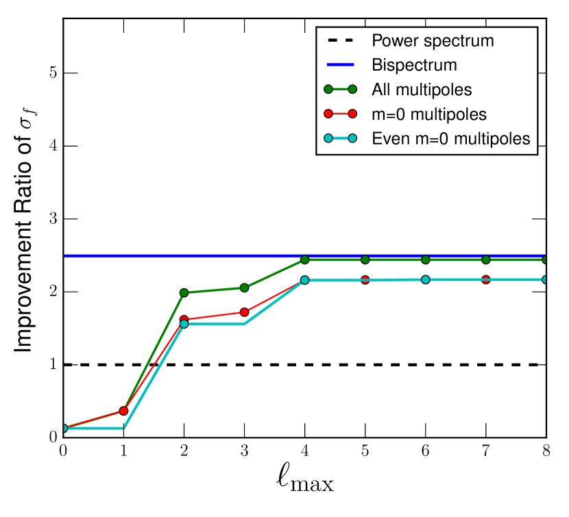
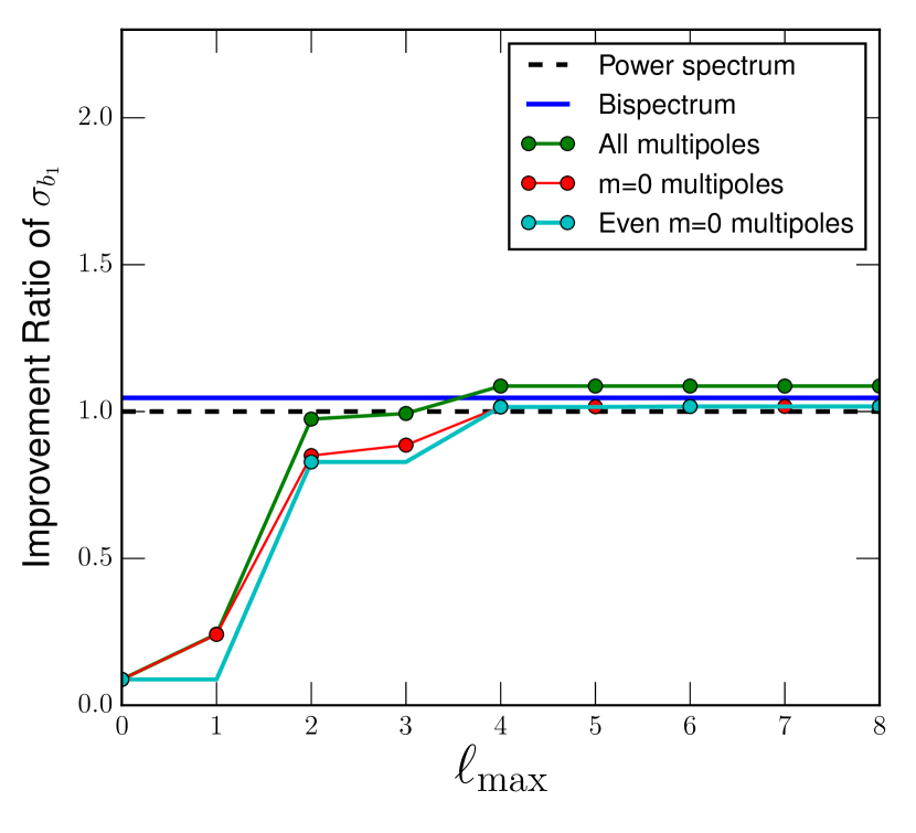
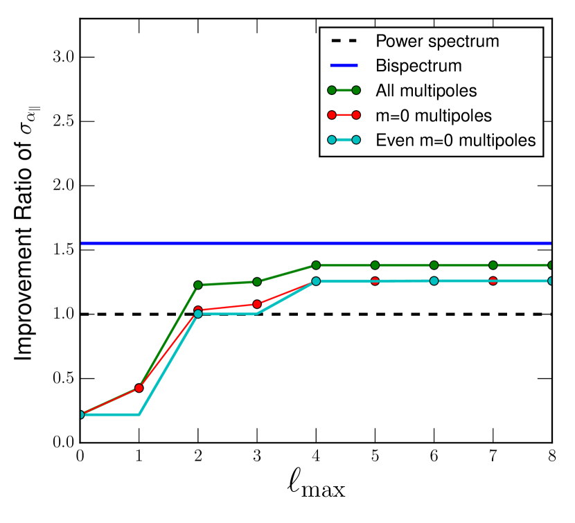
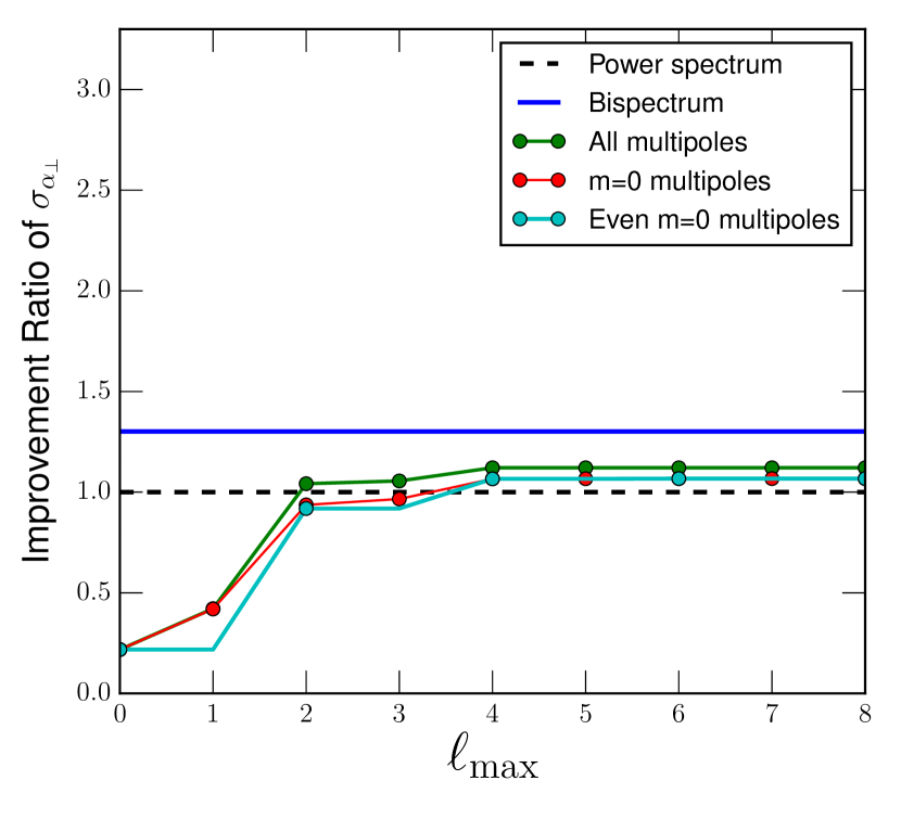
Figure 1: Cosmological constraints expected from the bispectrum multipoles as a function of maximum $\ell$ used in the analysis for a sample of DESI LRGs in $0.6<z<0.7$. The constraints from power spectrum and the full bispectrum are also displayed for comparison. The results are normalized to the expected power spectrum constraints so that the ordinate axis is an improvement factor over the power spectrum. The multipole constraints can never be stronger than the full bispectrum constraints. Our top right panel is consistent with this within the numerical error associated with monte carlo integration.

Fig. 1 shows that the full (unreduced) bispectrum is capable of providing better constraints compared to the power spectrum. This is especially true for the growth rate parameter $f$ where the improvement is almost a factor of 2 in the statistical errors. For the $\alpha$ parameters the constraints derived from the full bispectrum are still a factor of about 1.5 better compared to the power spectrum, but become slightly worse for the multipoles. In all cases the information in the multipoles seems to be mostly in the first three even $\ell$ modes with $m=0$.

The behaviour seems to be qualitatively similar for other redshifts and tracers. Fig. 2 shows similar results over a wider redshift range. This means that the first even multipoles averaged over azimuthal angle are as good as the full bispectrum for the purposes of deriving cosmological constraints.

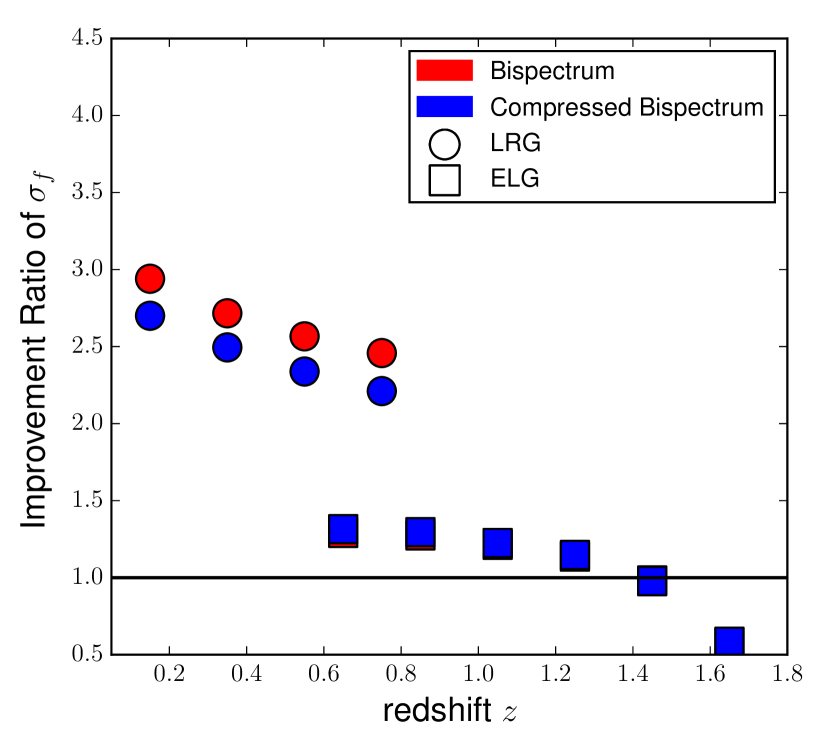
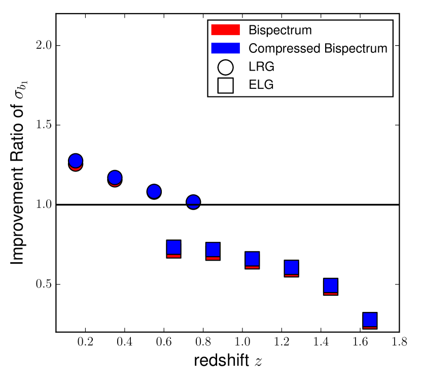
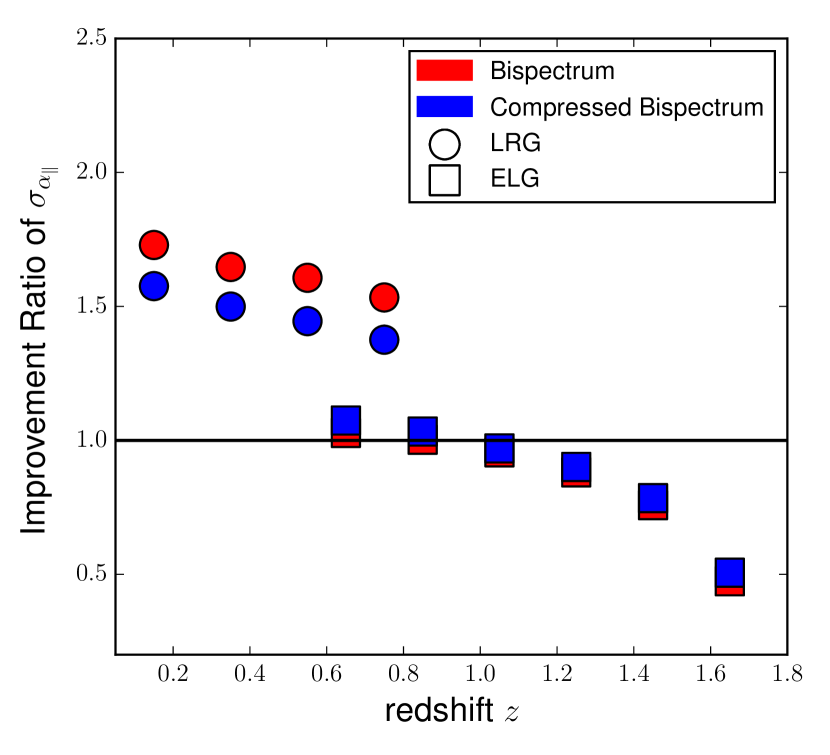
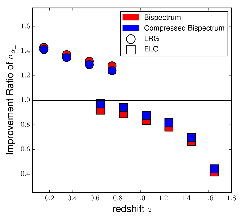
Figure 2: Improvement on derived errors of cosmological parameters compared to the power spectrum for different redshifts and tracer types. Red symbols (on top) represent the constraints derivable from the full bispectrum, while the blue symbols (on the bottom) represent constraints from first three even multipoles with $m=0$. For some redshifts the multipole constraints are slightly better than the full bispectrum constraints, but they are consistent within the numerical errors associated with the monte carlo integration.

The bispectrum provides significantly larger improvement over power spectrum at low redshifts. This is due to a high number density of galaxies and the higher amplitude of fluctuations.

6 Conclusions

We developed a Fisher information matrix based method of computing the expected constraints on cosmological parameters from the bispectrum and the angular multipoles of the bispectrum of a given galaxy sample. Since the full bispectrum is difficult to analyse, some kind of data reduction will inevitable have to be applied to the measurements. We computed the information loss associated with the commonly proposed reduction schemes that rely on angular integration of the bispectrum.

We find that the full bispectrum alone can deliver cosmological constraints that are a factor of few better than the ones derivable from the power spectrum at low $z$. The improvement is especially large for the growth rate parameter $f$ where the improvement on the measurement error is almost a factor of 3. The improvement is the largest at lower redshifts where the number density of galaxies in the sample is the highest. Most of the information is in the first three even multipoles with $m=0$, which means that just three numbers per bispectrum shape are enough for the purposes of obtaining cosmological constraints.

Our results at first may seem to contradict previously published results that claim a more modest improvement when adding the bispectrum to the power spectrum (Sefusatti & Komatsu, 2007; Szapudi, 2009; Carron & Neyrinck, 2012; Carron & Szapudi, 2014). This is due to a number of reasons. Many previous works have looked at the monopole of the bispectrum which will obviously contain much less information on $f$. The bispectrum information increases more steeply compared to the power spectrum with the number density of galaxies, therefore this large improvement will only result in future dense surveys and will not necessarily show in current and past surveys that have a lower galaxy number density. Finally, many past claims refer to “amplitude like” parameters (e.g. primordial amplitude of fluctuations) for isotropic fields. The $f$ parameter is not really “amplitude like” since it describes an angular dependent variations in the statistics, and the 5D shape of the bispectrum turns out to be more sensitive to this parameter than it would be to a mere change in amplitude.

Our results are consistent with the ones reported in Song et al. (2015) if we only consider strictly linear scales of $k_{i}<0.1\ \mathrm{Mpc/h}$. This is expected since the bispectrum signal to noise scales better with increasing $k_{\mathrm{max}}$ compared to the power spectrum. Their model includes the Finger of God effects and therefore the forecasts are more conservative and realistic. Since our main goal was not to produce accurate forecasts but rather to study the effects of the multipole reduction we decided to sacrifice the realism of constraints for clarity. We explicitly checked that our main conclusions are robust with respect to the choice of $k_{\mathrm{max}}$ and do not change when we include $\sigma_{\mathrm{FOG}}$.

In this work we do not consider a cross correlation between the power spectrum and the bispectrum measurements and it is difficult to say how big the overall improvement in the errors is when the two are properly combined (see Song et al., 2015, for correlated full bispectrum DESI forecasts). We know however that the improvement will be at least as big as the improvement from the bispectrum (or the bispectrum multipoles) alone. Recent studies indicated that the cosmological constraints from power spectrum and bispectrum are not very strongly correlated (Slepian & Eisenstein, 2016; Slepian et al., 2016; Gil-Marín et al., 2016), so the improvement may actually be much larger.

The main conclusions from our work are as follows:

• The bispectrum measurements from future surveys have a potential of improving the growth rate measurements by at least a factor of 2.5 at low redshifts (this is a very conservative estimate assuming that the bispectrum information is perfectly correlated with the power spectrum).

• When expanding the bispectrum in angular multipoles, the three numbers corresponding to the first three even terms with $m=0$ in the multipole expansion contain most of the information relevant for the derivation of cosmological constraints.

References

- Ade et al. (2014) Ade P., et al., 2014, Astronomy & Astrophysics, 571, A16
- Albrecht et al. (2006) Albrecht A., et al., 2006, arXiv preprint astro-ph/0609591
- Alcock & Paczynski (1979) Alcock C., Paczynski B., 1979, Nature, 281, 358
- Ballinger et al. (1996) Ballinger W., Peacock J., Heavens A., 1996, arXiv preprint astro-ph/9605017
- Beutler et al. (2014) Beutler F., et al., 2014, Monthly Notices of the Royal Astronomical Society, 443, 1065
- Carron & Neyrinck (2012) Carron J., Neyrinck M. C., 2012, ApJ, 750, 28
- Carron & Szapudi (2014) Carron J., Szapudi I., 2014, MNRAS, 439, L11
- Feldman et al. (1993) Feldman H. A., Kaiser N., Peacock J. A., 1993, arXiv preprint astro-ph/9304022
- Gil-Marín et al. (2015) Gil-Marín H., Noreña J., Verde L., Percival W. J., Wagner C., Manera M., Schneider D. P., 2015, Monthly Notices of the Royal Astronomical Society, 451, 5058
- Gil-Marín et al. (2016) Gil-Marín H., Percival W. J., Verde L., Brownstein J. R., Chuang C.-H., Kitaura F.-S., Rodríguez-Torres S. A., Olmstead M. D., 2016, arXiv preprint arXiv:1606.00439
- Greig et al. (2013) Greig B., Komatsu E., Wyithe J. S. B., 2013, Monthly Notices of the Royal Astronomical Society, 431, 1777
- Jackson (1972) Jackson J., 1972, Monthly Notices of the Royal Astronomical Society, 156, 1P
- Kaiser (1987) Kaiser N., 1987, Monthly Notices of the Royal Astronomical Society, 227, 1
- Kazin et al. (2010) Kazin E. A., et al., 2010, The Astrophysical Journal, 710, 1444
- Laureijs et al. (2011) Laureijs R., et al., 2011, arXiv preprint arXiv:1110.3193
- Levi et al. (2013) Levi M., et al., 2013, arXiv preprint arXiv:1308.0847
- Peebles (1980) Peebles P. J. E., 1980, The large-scale structure of the universe. Princeton university press
- Samushia et al. (2011) Samushia L., et al., 2011, Monthly Notices of the Royal Astronomical Society, 410, 1993
- Schlegel et al. (2009) Schlegel D. J., et al., 2009, arXiv preprint arXiv:0904.0468
- Scoccimarro (2000) Scoccimarro R., 2000, The Astrophysical Journal, 544, 597
- Scoccimarro (2015) Scoccimarro R., 2015, Physical Review D, 92, 083532
- Scoccimarro et al. (1999) Scoccimarro R., Couchman H., Frieman J. A., 1999, The Astrophysical Journal, 517, 531
- Sefusatti & Komatsu (2007) Sefusatti E., Komatsu E., 2007, Phys. Rev. D, 76, 083004
- Sefusatti et al. (2006) Sefusatti E., Crocce M., Pueblas S., Scoccimarro R., 2006, Physical Review D, 74, 023522
- Sefusatti et al. (2012) Sefusatti E., Crocce M., Desjacques V., 2012, Monthly Notices of the Royal Astronomical Society, 425, 2903
- Simpson & Peacock (2010) Simpson F., Peacock J. A., 2010, Physical Review D, 81, 043512
- Slepian & Eisenstein (2016) Slepian Z., Eisenstein D. J., 2016, arXiv preprint arXiv:1607.03109
- Slepian et al. (2016) Slepian Z., et al., 2016, arXiv preprint arXiv:1607.06097
- Song et al. (2015) Song Y.-S., Taruya A., Oka A., 2015, Journal of Cosmology and Astroparticle Physics, 2015, 007
- Szapudi (2009) Szapudi I., 2009, in Martínez V. J., Saar E., Martínez-González E., Pons-Bordería M.-J., eds, Lecture Notes in Physics, Berlin Springer Verlag Vol. 665, Data Analysis in Cosmology. pp 457–492, doi:10.1007/978-3-540-44767-2_14
- Taruya et al. (2011) Taruya A., Saito S., Nishimichi T., 2011, Physical Review D, 83, 103527
- Taylor & Hamilton (1996) Taylor A., Hamilton A., 1996, Monthly Notices of the Royal Astronomical Society, 282, 767
- Tegmark (1997) Tegmark M., 1997, Physical Review Letters, 79, 3806
- Tellarini et al. (2016) Tellarini M., Ross A. J., Tasinato G., Wands D., 2016, J. Cosmology Astropart. Phys., 6, 014
- Yamamoto et al. (2006) Yamamoto K., Nakamichi M., Kamino A., Bassett B. A., Nishioka H., 2006, Publications of the Astronomical Society of Japan, 58, 93