A systematic search for X-ray cavities in galaxy clusters, groups, and elliptical galaxies

Abstract

We perform a comprehensive study of X-ray cavities using a large sample of X-ray targets selected from the Chandra archive. The sample is selected to cover a large dynamic range including galaxy clusters, groups, and individual galaxies. Using $\beta$-modeling and unsharp masking techniques, we investigate the presence of X-ray cavities for 133 targets that have sufficient X-ray photons for analysis. We detect 148 X-ray cavities from 69 targets and measure their properties, including cavity size, angle, and distance from the center of the diffuse X-ray gas. We confirm the strong correlation between cavity size and distance from the X-ray center similar to previous studies (i.e., Bîrzan et al., 2004; Diehl et al., 2008; Dong et al., 2010). We find that the detection rates of X-ray cavities are similar among galaxy clusters, groups and individual galaxies, suggesting that the formation mechanism of X-ray cavities is independent of environment.

1. INTRODUCTION

The empirical scaling relations between supermassive black holes (SMBHs) and their host galaxy properties imply the coevolution of SMBHs and galaxies (e.g., Magorrian et al., 1998; Ferrarese & Merritt, 2000; Gebhardt et al., 2000; Kormendy & Ho, 2013; Woo et al., 2013), while understanding the nature of the coevolution remains as one of the important open questions. Representing the mass-accreting phase of SMBHs, active galactic nuclei (AGNs) have been considered as playing a crucial role through feedback in galaxy evolution. AGN activities may quench or enhance star formation as several simulations demonstrated both negative feedback (Kauffmann & Haehnelt, 2000; Granato et al., 2004; Di Matteo et al., 2005; Springel et al., 2005; Bower et al., 2006; Croton et al., 2006; Hopkins et al., 2006; Ciotti et al., 2010; Scannapieco et al., 2012), and positive feedback (Silk, 2005; Gaibler et al., 2012; Zubovas et al., 2013; Ishibashi et al., 2013).

Various observational studies have revealed evidence for AGN feedback (Fabian, 2012; Heckman & Best, 2014, and references therein), which occurs mainly in two modes, radiative (quasar) mode and kinetic (radio) mode. The radiative mode is related to the radiation pressure from the accretion disk, while the kinetic mode is caused by the mechanical power of radio jets.

The radiative mode is manifested in many different ways. Ionized gas outflows are typically observed in type 1 and type 2 AGNs (e.g., Crenshaw et al., 2003; Nesvadba et al., 2008, 2011; Woo et al., 2015). Winds are detected very close to the central region based on the kinematic features of narrow absorption lines in X-ray (Pounds et al., 2003; Tombesi et al., 2010) and broad absorption lines in UV (Weymann et al., 1991; Crenshaw et al., 2003; Ganguly et al., 2007). The asymmetric and blueshifted line profiles of C IV have been suggested as evidence for an AGN wind (i.e., Sulentic et al., 2000; Wang et al., 2011). At larger scales, velocity dispersions and shifts of emission lines in both ionized and molecular gas suggest AGN winds on scales comparable to that of the host galaxy (Boroson, 2005; Komossa et al., 2008; Barbosa et al., 2009; Bae & Woo, 2014; Woo et al., 2015).

In contrast, the radio mode feedback has been investigated in more massive systems at much larger scales. The radio mode feedback has been invoked to reconcile the cooling flow problem, i.e. that the observed cooling rate of hot gas in the central regions of galaxies and galaxy clusters is lower than the predicted value from cooling flow models (see Fabian 1994). A natural explanation is the existence of a heating source that prevents the cooling of the hot gas. AGNs have been considered as one possible candidate for heating (see McNamara & Nulsen 2007; Fabian 2012; Gitti et al. 2012 for review). Several studies based on simulations showed that AGN jets can provide sufficient energy to affect galaxy evolution and resolve the cooling flow problem (e.g., Sijacki & Springel, 2006; Dubois et al., 2010; Gaspari et al., 2012).

Based on the high-resolution X-ray imaging obtained with the Chandra and XMM-Newton telescopes, surface brightness depressions of diffuse X-ray emission have been detected at the centers of a number of massive galaxies and galaxy clusters, e.g., Abell 426 (Fabian et al. 2000, 2006), Hydra A (McNamara et al., 2000; Nulsen et al., 2005b; Wise et al., 2007), M87 (Churazov et al., 2001; Forman et al., 2007), Abell 2052 (Blanton et al., 2011), MS0735+7421 (McNamara et al., 2005), Abell 2199 (Johnstone et al., 2002), and Centaurus Cluster (Sanders & Fabian, 2002). These so-called X-ray cavities extend up to several hundred kpc (i.e., MS 0735.6+7421), exceeding the optical size of their host galaxies. Such cavities are considered a signpost of radio mode feedback, as they are often filled with radio lobes, implying that the cavities originate from the interaction between radio jets and interstellar/intergalactic medium (e.g., McNamara et al., 2000; Fabian et al., 2002; McNamara et al., 2005; Giacintucci et al., 2011; Chon et al., 2012). In general, observational studies found that the estimated jet energy inferred from the X-ray cavities can balance the cooling of hot gas (e.g., Bîrzan et al., 2004; Rafferty et al., 2006; Nulsen et al., 2009; Hlavacek-Larrondo et al., 2012). Thus, studying the physical properties of X-ray cavities can shed light on understanding AGN feedback and galaxy evolution.

To understand the nature of X-ray cavities, a number of studies have investigated their properties using samples of galaxies, groups, and clusters. For example, by detecting X-ray cavities from 14 galaxy clusters, one galaxy group, and one galaxy, Bîrzan et al. (2004) presented the relationship between X-ray cavity size and the distance from X-ray center. Diehl et al. (2008) expanded the sample size to 32 objects (30 galaxy clusters, one galaxy group, and one galaxy) and found a similar trend between cavity size and distance from the center. Dunn & Fabian (2006) suggested that the AGN feedback duty cycle is $\sim$ 70% based on the X-ray cavities detected from 14 galaxy clusters among a sample of 20 cool-core clusters. There have also been statistical studies for smaller scale systems such as galaxy groups and elliptical galaxies. For example, Dong et al. (2010) detected X-ray cavities in 26 galaxy groups, and showed that these systems follow the same size-distance relation found in galaxy clusters. X-ray cavities were also detected in giant elliptical galaxies (e.g., 24 objects out of 104 galaxies, Nulsen et al., 2009). Based on the detection rates of X-ray cavities in various environments, Dong et al. (2010) discussed the dependence of AGN feedback duty cycle on environments (i.e., galaxy clusters, galaxy groups, and isolated elliptical galaxies)

Recent work increased the number of known objects with X-ray cavities. Panagoulia et al. (2014) identified X-ray cavities from 30 out of 49 local galaxy groups and clusters, which have a cool-core at the central region. On the other hand, Hlavacek-Larrondo et al. (2012) detected X-ray cavities in 20 objects, using 76 massive clusters at higher redshifts ($0.3<z<0.7$). Also, Hlavacek-Larrondo et al. (2015) detected X-ray cavities from 6 objects among 83 galaxy clusters selected with the South Pole Telescope ($0.4<z<1.2$). Using the size of the cavities, Hlavacek-Larrondo et al. (2012, 2015) claimed that there is no evolution in radio mode feedback in at least the last $\sim$ 7 Gyr.

While a number of previous studies reported X-ray cavity detections using various samples, it is difficult to statistically investigate the physical properties of X-ray cavities as a population due to the incompleteness and various selection functions of individual studies. For example, the sample size of Dong et al. (2010); Hlavacek-Larrondo et al. (2012); Panagoulia et al. (2014) studies is relatively large (i.e., 51, 76, and 49 objects, respectively), reporting discovery of a number of new X-ray cavities. However, a large fraction of the targets in these surveys do not have sufficient photon counts to properly study the presence of X-ray cavities.

In this paper, we present the results from our X-ray cavity study based on a large sample of targets, for which diffuse X-ray emission is detected in the $Chandra$ X-ray images. Our sample also covers a large dynamic range from isolated galaxies to galaxy clusters. By adopting a consistent X-ray photon number criterion, we analyze X-ray images in order to detect X-ray cavities, measure their properties, and investigate the dependence of the cavity formation on environments. We describe the sample selection and data reduction in §2, and the detection method and analysis in §3. The main results are presented in §4, followed by discussion in §5, and summary and conclusions in §6. We adopt a cosmology of $H_{\rm 0}=70$ km s^-1 Mpc^-1, $\Omega_{\Lambda}=0.7$ and $\Omega_{\rm m}=0.3$.

2. Sample and data

To search X-ray cavities, we used available $Chandra$ X-ray images, which provide high spatial resolution (PSF FWHM $\sim$0$\farcs$5 at the aim point), ideal for X-ray cavity studies. We considered sources in the $Chandra$ archive in one of three categories, namely, ‘normal galaxies’, ‘cluster of galaxies’, and ‘active galaxies and quasar’. Using these categories enables us to cover a large dynamical range. We selected a parent sample of $\sim$3500 targets, for which 5472 individual exposures are available, including multiple images per target (i.e., 2668, 1071, and 1733 exposures of active galaxies and quasars, normal galaxies, and cluster of galaxies respectively). For our cavity study, we used a final sample of 133 targets based on a consistent analysis of X-ray photon counts as described below.

To detect surface brightness depression, a sufficient number of X-ray photons is required. In a previous study, Dong et al. (2010) discussed the conditions of X-ray cavity detection based on simulations with various parameters (e.g., radial profile $\beta$, total photon count, cavity strength, and distance from the center), concluding that total photon count is the most important parameter for X-ray cavity detection. However, we found that the total photon count is not a reliable criterion for sample selection since it strongly depends on the spatial distribution of the diffuse emission. For example, if the diffuse X-ray photons are spread out with an average small photon count per pixel, it is difficult to detect cavities although the total photon count is large. On the other hand, if the photon count is high at the central part, then cavities can be detected although the total photon count is small. Thus, we concluded that the total photon count does not provide a consistent selection condition.

Instead of the total photon count, we focused on the photon counts in the diffuse gas near the center of the image. Many targets show an X-ray AGN at the center, hence, the count from the point source contributes to the total count, contaminating the diffuse gas emission. To avoid this contamination, we decided to use an annulus to measure the photon counts for selecting targets of further analysis. Since the center of the diffuse emission is typically close to the aim point of ACIS, we used the size of the PSF FWHM $\sim$2 pixel (i.e., 0.984 ″), which is relevant for most of energy bands. While for some targets, the diffuse emission is off from the aim point and the PSF size varies as a function of distance from the aim point, we assumed PSF size is 2 pixels for all images since we performed PSF deconvolution as described later in this section.

The contribution of the point source decreases outwards, becoming $\sim$1% of the peak value at the distance of 3 pixels in the Chandra PSF. We conservatively adopted an annulus with an inner radius of 6 and the outer radius of 7 pixels to calculate the mean count per pixel within the annulus. After that, we selected targets if the mean X-ray photon count of the annulus is larger than 4 counts per pixel, which corresponds to Poisson noise of 2.

Since the sample size is very large, we initially selected targets with enough X-ray photons by examining the 4$\times$4 pixel binned images, which was intended to increase the S/N ratio. We excluded targets if diffuse X-ray emission is not visible, for which the photon count corresponds to 2-3 counts per pixel (i.e., 0.1-0.2 counts per unbinned pixel). In other words, these excluded images obviously have a far lower photon count that 4 counts per pixel. Thus, this initial selection conservatively reduced target sample size to $\sim$800 objects. Note that although we checked the individual images in this process, we also checked that if multiple exposures are available, the combined images of these excluded targets do not have sufficient photon counts.

For the selected $\sim$800 targets, we performed more detailed analysis after PSF deconvolution. Since the PSF of Chandra images varies along with the spatial location from $\sim$0$\farcs$5 to a few arcseconds, relatively small cavities far from the center can be affected by the effect of the PSF. To deconvolve the PSF of each image, we reduced raw data using the ”Chandra_repro” script of the Chandra Interactive Analysis of Observations software (CIAO) v4.6 and Chandra Calibration Database (CALDB) 4.6.3. This script performs all reduction processes such as ”acis_process_event”, including charge transfer inefficiency correction, time-dependent gain adjustment, and screening for bad pixels using the bad pixel map in the pipeline. After reduction process, we generated count images and exposure-corrected images in the 0.5-7 keV energy band, using ”$\rm fluximage$” script as well as the PSF map using ”mkpsfmap” script. Based on the count image and the PSF map, we performed the PSF deconvolution, using ”deconvblind” function of MATLAB. The majority of the targets in the sample are observed at the aim point, hence the PSF effect is negligible for cavity detection. In contrast, if diffuse emission is far from the aim point, the PSF- deconvolved images significantly improve the detection of X-ray cavities. Once the PSF deconvolution is complete, then we combined individual exposures to improve S/N whenever multiple images are available per target.

After PSF deconvolution and combining exposures, we measured the photon counts at the annulus (6-7) and selected objects with more than 4 counts. With these criteria, we finalized a sample of 133 targets, which is composed of isolated elliptical galaxies, galaxy groups, and galaxy clusters, covering a range of gas temperatures and various environments (i.e., from 0.3 to 10 keV, which are typical temperature of an isolated elliptical galaxy and a massive galaxy cluster, respectively). This sample is the largest to date for investigating X-ray cavities over a broad dynamic range, enabling a comprehensive study of X-ray cavities and their formation and evolution in different environments. The details of our targets are presented in Table 1. Note that we use exposure-corrected images for cavity analysis while we use count images for sample selection.

In the sample selection, we have excluded several objects although these objects satisfied our photon count criteria. First, we excluded spiral galaxies (i.e., M31) and starburst galaxies (i.e., NGC253, M82), since diffuse X-ray emission for those target is due to evolved star or supernova (e.g., Strickland et al., 2000, 2004; Bogdán & Gilfanov, 2008). Second, we excluded merging clusters, which show strongly disturbed distributions (e.g., bullet cluster), using the three lists, namely, ”MCC Radio Relic Sample”, ”MCC Chandra-Planck Merging Cluster Sample”, and ”Other Proven Dissociative Mergers”, from the merging cluster collaboration. Note that we did not exclude two objects (Abell 2146 and Cygnus A) in ”Other merging clusters” since they are not classified as dissociative.

Diffuse X-ray emission mainly originates from hot gas, although other sources may contribute, i.e., cataclysmic variables and coronally active binary stars. The X-ray luminosity of these additional sources is less than $10^{34}\ \rm erg\ s^{-1}$ (e.g., Sazonov et al., 2006), corresponding to $\sim 0.2$ counts in total for 200 ks exposure at the distance of the closest target (NGC 4552), which is based on the calculation, using the Chandra X-Ray Center Portable, Interactive, Multi-Mission Simulator software. Due to PSF effects, the photon count per pixel will be even smaller. Thus, contamination from these additional X-ray sources is negligible for our extragalactic sources.

Since we selected X-ray targets with sufficient photon counts at the central part of the targets, the sample may be biased to cool-core clusters, which are known to have high surface brightness (e.g., Panagoulia et al., 2014). We calculated the cooling time of each target to investigate whether the cooling time is sufficiently short. We adopted the method given by Equation 14 of Hudson et al. (2010), which calculates cooling time using the density of ions, electrons, hydrogen, and temperature derived from $\rm 0.004\ R_{500}$ and the cooling function. A spectrum for each target is extracted within $\rm 0.004\ R_{500}$, excluding the central region with a 6 pixel radius to remove the AGN contribution, as similarly used in the sample selection. Here, we used ”specextract” script of CIAO with the longest exposure for each target for simplicity while $\rm R_{500}$ was estimated using Equation 12 of Vikhlinin et al. (2006). Since the $\rm R_{500}$ and gas temperature are dependent on each other, we estimated them with iterations. The detailed method to estimate $\rm R_{500}$ and gas temperature will be presented in §3.4. Then, we fitted the spectra using XSPEC (version 12.8.2) with a single temperature plasma model (MEKAL) and hydrogen gas absorption model (WABS), with gas temperature, normalization factor, and metal abundance as free parameters. We generally treated galactic absorption as a free parameter, except for a few sources where we adopted galactic HI column density from Dickey & Lockman (1990) since the parameter did not converge to reliable values due to the low photon counts. Based on the normalization factor, we calculated electron density and hydrogen density assuming that the ratio of electrons to hydrogen is 1.2 and that hydrogen and ions have the same density. Finally, the cooling function was adopted from Sutherland & Dopita (1993) and interpolated for our estimated metal abundances and gas densities. In summary, we found that the cooling time of all targets is not larger than 3 Gyrs, suggesting that in general our targets have cool cores at the centers.

Table 1Target list

Object	RA	DEC	z	$N_{H}$	T	Class
				($10^{20}\rm{cm^{-2}}$)	(keV)
(1)	(2)	(3)	(4)	(5)	(6)	(7)
Abell 426	03 : 19 : 44	41 : 25 : 19	$0.018$	13.66	$3.61_{-0.01}^{+0.01}$	1
NGC 1316	03 : 22 : 42	-37 : 12 : 29	$0.006$	5.32	$0.74_{-0.03}^{+0.03}$	1
2A 0335+096	03 : 38 : 41	09 : 58 : 05	$0.036$	24.38	$1.98_{-0.01}^{+0.01}$	1
Abell 478	04 : 13 : 25	10 : 27 : 58	$0.088$	33.76	$4.80_{-0.06}^{+0.06}$	1
MS 0735.6+7421	07 : 41 : 50	74 : 14 : 53	$0.216$	2.51	$4.15_{-0.10}^{+0.10}$	1
HYDRA A	09 : 18 : 06	-12 : 05 : 46	$0.055$	4.73	$3.44_{-0.03}^{+0.06}$	1
RBS 797	09 : 47 : 13	76 : 23 : 17	$0.354$	5.33	$5.07_{-0.15}^{+0.16}$	1
M84	12 : 25 : 04	12 : 53 : 13	$0.003$	7.99	$0.74_{-0.02}^{+0.02}$	1
M87	12 : 30 : 50	12 : 23 : 31	$0.004$	7.47	$1.72_{0.00}^{+0.00}$	1
NGC 4552	12 : 35 : 37	12 : 32 : 38	$0.001$	2.57*	$0.63_{-0.03}^{+0.03}$	1
NGC 4636	12 : 42 : 50	02 : 41 : 17	$0.003$	3.67	$0.76_{0.00}^{+0.00}$	1
Centaurus cluster	12 : 48 : 49	-41 : 18 : 43	$0.011$	12.36	$2.06_{0.00}^{+0.00}$	1
HCG 62	12 : 53 : 06	-09 : 12 : 22	$0.015$	11.86	$0.96_{0.00}^{+0.00}$	1
NGC 5044	13 : 15 : 24	-16 : 23 : 06	$0.009$	10.34	$0.98_{0.00}^{+0.00}$	1
Abell 3581	14 : 07 : 30	-27 : 01 : 05	$0.023$	6.95	$1.63_{-0.01}^{+0.01}$	1
NGC 5813	15 : 01 : 07	01 : 41 : 02	$0.007$	6.37	$0.72_{0.00}^{+0.00}$	1
Abell 2052	15 : 16 : 44	07 : 01 : 16	$0.035$	5.40	$2.37_{-0.01}^{+0.01}$	1
3C 320	15 : 31 : 25	35 : 33 : 40	$0.342$	3.78	$3.27_{-0.23}^{+0.25}$	1
Cygnus A	19 : 59 : 28	40 : 44 : 02	$0.056$	32.44	$5.54_{-0.08}^{+0.08}$	1
PKS 2153-69	21 : 57 : 06	-69 : 41 : 24	$0.028$	2.5*	$1.98_{-0.04}^{+0.04}$	1
3C 444	22 : 14 : 26	-17 : 01 : 37	$0.153$	2.43	$1.90_{-0.04}^{+0.04}$	1
Abell 85	00 : 41 : 42	-09 : 20 : 53	$0.055$	5.29	$4.65_{-0.07}^{+0.07}$	2
ZwCl 0040+2404	00 : 43 : 52	24 : 24 : 22	$0.083$	5.51	$2.73_{-0.07}^{+0.09}$	2
ZwCl 0104+0048	01 : 06 : 49	01 : 03 : 22	$0.255$	3.13	$2.79_{-0.10}^{+0.09}$	2
NGC 533	01 : 25 : 31	01 : 45 : 32	$0.019$	12.41	$1.02_{-0.01}^{+0.01}$	2
Abell 262	01 : 52 : 47	36 : 09 : 07	$0.017$	10.37	$1.62_{-0.01}^{+0.01}$	2
MACS J0242.5-2132	02 : 42 : 36	-21 : 32 : 28	$0.314$	4.45	$4.13_{-0.23}^{+0.26}$	2
Abell 383	02 : 48 : 03	-03 : 31 : 41	$0.187$	2.60	$3.77_{-0.15}^{+0.15}$	2
AWM 7	02 : 54 : 28	41 : 34 : 44	$0.017$	10.62	$3.79_{-0.05}^{+0.05}$	2
MACS J0329.6-0211	03 : 29 : 40	-02 : 11 : 38	$0.450$	5.11	$5.00_{-0.36}^{+0.39}$	2
NGC 1399	03 : 38 : 11	-35 : 41 : 53	$0.005$	48.92	$0.31_{-0.02}^{+0.03}$	2
NGC 1404	03 : 38 : 52	-35 : 35 : 35	$0.006$	1.36*	$0.78_{-0.01}^{+0.01}$	2
RXC J0352.9+1941	03 : 52 : 59	19 : 40 : 59	$0.109$	14.49	$2.00_{-0.04}^{+0.04}$	2
MACS J0417.5-1154	04 : 17 : 35	-11 : 54 : 32	$0.440$	4.08	$6.31_{-0.40}^{+0.42}$	2
RX J0419.6+0225	04 : 19 : 34	02 : 28 : 23	$0.012$	16.03	$1.32_{0.00}^{+0.00}$	2
EXO 0423.4-0840	04 : 25 : 51	-08 : 33 : 40	$0.038$	17.68	$2.05_{-0.09}^{+0.08}$	2
Abell 496	04 : 33 : 38	-13 : 15 : 43	$0.033$	4.58	$4.15_{-1.72}^{+1.72}$	2
RXC J0439.0+0520	04 : 39 : 02	05 : 20 : 42	$0.208$	12.54	$3.60_{-0.22}^{+0.21}$	2
MS 0440.5+0204	04 : 43 : 10	02 : 10 : 19	$0.190$	15.97	$4.36_{-0.19}^{+0.25}$	2
MACS J0744.9+3927	07 : 44 : 53	39 : 27 : 29	$0.698$	5.30	$10.30_{-1.50}^{+2.75}$	2
PKS 0745-19	07 : 47 : 32	-19 : 17 : 46	$0.103$	41.49	$5.12_{-0.04}^{+0.04}$	2
ZwCl 0949+5207	09 : 52 : 49	51 : 53 : 06	$0.214$	2.21	$4.25_{-0.09}^{+0.11}$	2
ZwCl 1021+0426	10 : 23 : 39	04 : 11 : 13	$0.285$	2.72	$5.34_{-0.16}^{+0.24}$	2
RXC J1023.8-2715	10 : 23 : 50	-27 : 15 : 22	$0.253$	5.79	$5.06_{-0.17}^{+0.18}$	2
Abell 1068	10 : 40 : 44	39 : 57 : 11	$0.138$	1.20	$4.39_{-0.10}^{+0.10}$	2
Abell 1204	11 : 13 : 18	17 : 36 : 11	$0.171$	3.70	$3.47_{-0.11}^{+0.13}$	2
NGC 4104	12 : 06 : 38	28 : 10 : 26	$0.028$	8.57	$1.57_{-0.05}^{+0.04}$	2
NGC 4472	12 : 29 : 47	08 : 00 : 14	$0.003$	9.46	$1.00_{0.00}^{+0.00}$	2
Abell 1689	13 : 11 : 30	-01 : 20 : 31	$0.183$	4.20	$9.29_{-0.34}^{+0.34}$	2
RX J1350.3+0940	13 : 50 : 22	09 : 40 : 12	$0.090$	2.59	$3.07_{-0.10}^{+0.11}$	2
ZwCl 1358+6245	13 : 59 : 51	62 : 31 : 05	$0.329$	3.62	$5.20_{-0.33}^{+0.49}$	2
Abell 1835	14 : 01 : 02	02 : 52 : 44	$0.253$	3.33	$5.61_{-0.11}^{+0.11}$	2
MACS J1423.8+2404	14 : 23 : 48	24 : 04 : 44	$0.543$	4.68	$4.77_{-0.19}^{+0.20}$	2
Abell 1991	14 : 54 : 31	18 : 38 : 31	$0.059$	6.53	$1.88_{-0.02}^{+0.02}$	2
RXC J1504.1-0248	15 : 04 : 08	-02 : 48 : 18	$0.215$	11.21	$5.18_{-0.09}^{+0.09}$	2
NGC 5846	15 : 06 : 29	01 : 36 : 22	$0.006$	10.39	$0.81_{-0.01}^{+0.01}$	2
MS 1512-cB58	15 : 14 : 22	36 : 36 : 25	$2.723$	2.42	$7.43_{-1.11}^{+1.09}$	2
RXC J1524.2-3154	15 : 24 : 13	-31 : 54 : 25	$0.103$	16.05	$2.65_{-0.03}^{+0.03}$	2
RX J1532.9+3021	15 : 32 : 54	30 : 21 : 00	$0.345$	2.52	$4.44_{-0.12}^{+0.12}$	2
Abell 2199	16 : 28 : 38	39 : 33 : 04	$0.030$	4.05	$3.68_{-0.04}^{+0.04}$	2
Abell 2204	16 : 32 : 47	05 : 34 : 34	$0.152$	10.78	$4.89_{-0.06}^{+0.06}$	2
NGC 6338	17 : 15 : 23	57 : 24 : 40	$0.027$	10.56	$1.68_{-0.02}^{+0.02}$	2
MACS J1720.3+3536	17 : 20 : 17	35 : 36 : 25	$0.391$	2.77	$5.38_{-0.43}^{+0.58}$	2
MACS J1931.8-2634	19 : 31 : 50	-26 : 34 : 34	$0.352$	9.84	$4.87_{-0.13}^{+0.14}$	2
MACS J2046.0-3430	20 : 46 : 01	-34 : 30 : 18	$0.423$	5.79	$4.65_{-0.38}^{+0.41}$	2
MACS J2229.7-2755	22 : 29 : 45	-27 : 55 : 37	$0.324$	3.65	$3.73_{-0.23}^{+0.24}$	2
Sersic 159-03	23 : 13 : 58	-42 : 43 : 34	$0.058$	4.53	$2.43_{-0.02}^{+0.02}$	2
Abell 2597	23 : 25 : 20	-12 : 07 : 26	$0.085$	3.27	$3.13_{-0.03}^{+0.03}$	2
Abell 2626	23 : 36 : 30	21 : 08 : 46	$0.055$	6.51	$2.79_{-0.04}^{+0.04}$	2
MACS J0159.8-0849	01 : 59 : 49	-08 : 49 : 59	$0.405$	5.71	$5.99_{-0.45}^{+0.48}$	3
NGC 1132	02 : 52 : 52	-01 : 16 : 34	$0.023$	11.78	$1.19_{-0.02}^{+0.02}$	3
Abell 3112	03 : 17 : 58	-44 : 14 : 17	$0.075$	4.66	$3.88_{-0.06}^{+0.06}$	3
NGC 1332	03 : 26 : 17	-21 : 20 : 10	$0.005$	18.49	$0.50_{-0.10}^{+0.06}$	3
NGC 1407	03 : 40 : 12	-18 : 34 : 48	$0.006$	14.99	$0.92_{-0.02}^{+0.02}$	3
4C+37.11	04 : 05 : 49	38 : 03 : 32	$0.055$	76.06	$3.66_{-0.07}^{+0.07}$	3
MACS J0429.6-0253	04 : 29 : 36	-02 : 53 : 06	$0.399$	5.90	$5.34_{-0.43}^{+0.57}$	2
RXC J0528.9-3927	05 : 28 : 56	-39 : 27 : 47	$0.284$	2.45	$7.00_{-0.53}^{+0.57}$	3
PLCKG266.6-27.3	06 : 15 : 52	-57 : 46 : 52	$0.972$	4.33	$14.02_{-1.57}^{+1.57}$	3
4C+55.16	08 : 34 : 55	55 : 34 : 23	$0.241$	6.45	$3.28_{-0.06}^{+0.06}$	3
MS 0839.9+2938	08 : 42 : 56	29 : 27 : 29	$0.194$	6.46	$3.30_{-0.13}^{+0.13}$	3
ZwCl 0857+2107	09 : 00 : 37	20 : 53 : 42	$0.235$	3.88	$3.13_{-0.09}^{+0.09}$	3
IRAS 09104+4109	09 : 13 : 46	40 : 56 : 28	$0.442$	2.67	$4.62_{-0.21}^{+0.22}$	3
Abell 907	09 : 58 : 22	-11 : 03 : 50	$0.153$	7.93	$4.78_{-0.16}^{+0.16}$	3
NGC 3402	10 : 50 : 27	-12 : 50 : 28	$0.015$	12.17	$0.93_{-0.01}^{+0.01}$	3
MACS J1115.8+0129	11 : 15 : 52	01 : 29 : 53	$0.352$	4.74	$5.37_{-0.29}^{+0.58}$	3
Abell 1361	11 : 43 : 40	46 : 21 : 22	$0.117$	5.24	$3.23_{-0.13}^{+0.13}$	3
Abell 1413	11 : 55 : 10	23 : 30 : 47	$0.143$	6.52	$6.59_{-0.19}^{+0.19}$	3
RX J1159.8+5531	11 : 59 : 51	55 : 32 : 02	$0.081$	6.65	$1.68_{-0.02}^{+0.02}$	3
MKW 4	12 : 04 : 27	01 : 53 : 42	$0.020$	7.92	$1.76_{-0.03}^{+0.03}$	3
NGC 4261	12 : 19 : 23	05 : 49 : 30	$0.007$	14.48	$0.73_{-0.02}^{+0.02}$	3
NGC 4649	12 : 43 : 40	11 : 33 : 11	$0.004$	13.12	$0.89_{0.00}^{+0.00}$	3
MRK 231	12 : 56 : 14	56 : 52 : 26	$0.042$	1.26*	$0.83_{-0.02}^{+0.02}$	3
Abell 1650	12 : 58 : 42	-01 : 45 : 43	$0.084$	3.71	$5.45_{-0.13}^{+0.18}$	3
Abell 1664	13 : 03 : 42	-24 : 14 : 46	$0.128$	10.23	$2.57_{-0.06}^{+0.06}$	3
MACS J1311.0-0311	13 : 11 : 02	-03 : 10 : 37	$0.494$	4.60	$4.47_{-0.39}^{+0.47}$	3
RX J1347.5-1145	13 : 47 : 31	-11 : 45 : 11	$0.451$	6.28	$10.46_{-0.45}^{+0.53}$	3
Abell 1795	13 : 48 : 53	26 : 35 : 28	$0.062$	2.03	$4.28_{-0.05}^{+0.07}$	3
MACS J1427.2+4407	14 : 27 : 16	44 : 07 : 30	$0.487$	3.21	$4.58_{-0.51}^{+0.52}$	3
RCS J1447+0828	14 : 47 : 27	08 : 28 : 19	$0.380$	5.46	$4.88_{-0.28}^{+0.29}$	3
MS 1455.0+2232	14 : 57 : 14	22 : 20 : 38	$0.258$	5.39	$4.25_{-0.09}^{+0.10}$	3
RXC J1459.4-1811	14 : 59 : 29	-18 : 10 : 44	$0.236$	9.89	$3.58_{-0.11}^{+0.11}$	3
Abell 2029	15 : 10 : 56	05 : 44 : 42	$0.077$	5.04	$6.23_{-0.05}^{+0.05}$	3
MKW 03S	15 : 21 : 52	07 : 42 : 32	$0.045$	5.13	$3.39_{-0.03}^{+0.03}$	3
Abell 2146	15 : 56 : 10	66 : 21 : 25	$0.234$	2.81*	$4.24_{-0.15}^{+0.17}$	3
Abell 2142	15 : 58 : 20	27 : 14 : 46	$0.091$	6.21	$7.19_{-0.13}^{+0.13}$	3
RXC J1558.3-1410	15 : 58 : 22	-14 : 09 : 58	$0.097$	12.28	$3.65_{-0.08}^{+0.08}$	3
ESO 137-006	16 : 15 : 04	-60 : 54 : 25	$0.018$	21.30	$0.99_{-0.15}^{+0.12}$	3
MACS J1621.3+3810	16 : 21 : 25	38 : 10 : 08	$0.465$	2.74	$5.00_{-0.57}^{+0.72}$	3
Abell 2219	16 : 40 : 20	46 : 42 : 40	$0.226$	3.19	$11.07_{-1.10}^{+1.36}$	3
Hercules A	16 : 51 : 08	04 : 59 : 35	$0.155$	7.18	$3.15_{-0.11}^{+0.11}$	3
Abell 2244	17 : 02 : 43	34 : 03 : 36	$0.097$	3.95	$5.16_{-0.10}^{+0.10}$	3
Ophiuchus cluster	17 : 12 : 28	-23 : 22 : 12	$0.028$	38.59	$7.40_{-0.15}^{+0.15}$	3
B3 1715+425	17 : 17 : 19	42 : 26 : 56	$0.183$	2.40	$4.24_{-0.31}^{+0.40}$	3
RXC J1720.1+2637	17 : 20 : 09	26 : 38 : 06	$0.164$	7.27	$4.80_{-0.16}^{+0.17}$	3
ZwCl 1742+3306	17 : 44 : 14	32 : 59 : 28	$0.076$	6.65	$2.92_{-0.05}^{+0.05}$	3
NGC 6482	17 : 51 : 49	23 : 04 : 19	$0.013$	13.93	$0.75_{-0.01}^{+0.01}$	3
H 1821+643	18 : 21 : 57	64 : 20 : 38	$0.297$	4.04*	$4.91_{-0.14}^{+0.14}$	3
NGC 6861	20 : 07 : 19	-48 : 22 : 12	$0.009$	6.95	$1.25_{-0.03}^{+0.03}$	3
PKS 2005-489	20 : 09 : 25	-48 : 49 : 55	$0.071$	3.08	$2.28_{-0.12}^{+0.14}$	3
RXC J2014.8-2430	20 : 14 : 52	-24 : 30 : 22	$0.161$	14.91	$4.05_{-0.09}^{+0.10}$	3
RX J2129.6+0005	21 : 29 : 40	00 : 05 : 20	$0.235$	3.98	$5.29_{-0.27}^{+0.37}$	3
MS 2137.3-2353	21 : 40 : 15	-23 : 39 : 40	$0.313$	4.96	$4.34_{-0.13}^{+0.16}$	3
Abell 2390	21 : 53 : 36	17 : 41 : 46	$0.228$	11.31	$5.92_{-0.15}^{+0.15}$	3
3C 438	21 : 55 : 52	38 : 00 : 29	$0.290$	29.76	$6.73_{-0.45}^{+0.56}$	3
IC 1459	22 : 57 : 11	-36 : 27 : 43	$0.006$	10.33	$0.57_{-0.16}^{+0.05}$	3
Abell 2550	23 : 11 : 37	-21 : 44 : 28	$0.123$	2.95	$2.00_{-0.06}^{+0.06}$	3
NGC 7618	23 : 19 : 47	42 : 51 : 07	$0.017$	22.33	$0.91_{-0.01}^{+0.01}$	3
NGC 7619	23 : 20 : 06	08 : 09 : 29	$0.013$	12.01	$0.88_{-0.02}^{+0.02}$	3
Abell 2589	23 : 23 : 57	16 : 46 : 41	$0.041$	4.65	$3.81_{-0.08}^{+0.08}$	3
RCS J2327-0204	23 : 27 : 28	-02 : 04 : 37	$0.700$	3.82	$8.66_{-0.85}^{+1.26}$	3
Abell 2627	23 : 36 : 42	23 : 55 : 05	$0.126$	4.31*	$3.80_{-0.39}^{+0.40}$	3
SPT-CL J2344-4243	23 : 44 : 42	-42 : 42 : 54	$0.620$	2.62	$7.47_{-0.73}^{+0.78}$	3
Abell 4059	23 : 57 : 00	-34 : 45 : 29	$0.049$	3.84	$3.22_{-0.03}^{+0.03}$	3
Note – Col. (1): Object name. Col. (2): RA. Col. (3): DEC. Col. (4): Redshift from NASA/IPAC
extragalactic database. Col. (5): HI column density. For targets with an asterisk, the quoted values are
from Dickey & Lockman (1990). Col. (6): Gas temperature. Col. (7): Class of X-ray cavity detection: 1:
X-ray cavities detected from raw images, 2: X-ray cavities detected from beta-model
subtracted images, 3: and X-ray cavities non-detected.

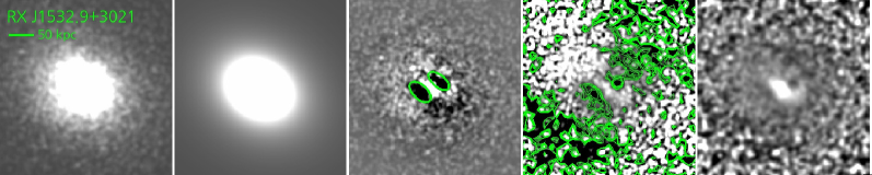
Figure 1.— Example of the $\beta$-model fitting result for RXJ1532.9+3021. Smoothed raw image (left), $\beta$-model (center left), residual image after subtracting $\beta$-model (center), normalized image with contour levels of 90%, 85%, 80%, 75%, 70% decreasing from outer to inner side (center right) and unsharp masked image (right).

3. Analysis

3.1. Detection method

To detect X-ray cavities, we used two methods, the $\beta$-modeling and the unsharp masking technique (see Figure 1), as previously used in other studies (e.g., Diehl et al., 2008; Dong et al., 2010). First, for $\beta$-modeling, the radial distribution of the surface brightness of diffuse X-ray gas is modeled assuming an isothermal distribution of the hot gas (Cavaliere & Fusco-Femiano, 1976). Using the $Sherpa$ package in CIAO, we fitted the surface brightness profile with various parameters, e.g., radius, ellipticity, and power-law index, as free parameters except for the location of the center of X-ray emission. We fixed the peak of the distribution as the center since many targets show asymmetric distribution (e.g., cold front). If we fit the center as a free parameter, the center is almost identical to the peak location within $\sim$1 pixel for the targets that show symmetric distribution (e.g., Abell 85, NGC 533, Abell 383), while for the targets with asymmetric distribution, the center is significantly off from the location of the peak by up to 60 pixels (e.g., Abell 2146, Ophiuchus cluster). To subtract background, we used constant value as representative of the background. We did not exclude the central bright point source (X-ray AGN) since masking or fitting the point source does not improve the results.

For the targets with strong and large X-ray cavities (21 objects), the $\beta$-model does not provide a good fit since the spatial profile dramatically changes (see Figure 2). Instead, we can directly detect cavities from the raw images, or use the unsharp masked image to identify cavities.

Second, we applied the unsharp masking technique by utilizing the smoothing task ”aconvolve” in CIAO. Adopting 2 pixels (i.e., 0.984″) for small scales and 10 pixels for large scales, we produced smoothed (small and large) images and divided the large scale smoothed image by the small scale smoothed image to obtain the unsharp masked image. A weakness of the unsharp masking technique is that it is difficult to determine the size of X-ray cavities because the size varies with smoothing lengths (see Dong et al., 2010). Also, for extreme cases, X-ray cavities are not detected from the unsharp masked image (e.g., NGC 533), while cavities are clearly detected from the $\beta$-modeling analysis (see Figure 3). Therefore, we mainly used the $\beta$-model to detect X-ray cavities, and used the unsharp masking technique as a secondary method.

In the detection process, we also used the normalized images which were generated by dividing a raw image by the best $\beta$-model, in order to conservatively define cavities more. By examining the normalized images as well as residual images, we investigated the spatial extent of relative depression. We require a minimum of 15% depression to confirm the presence of cavities and estimate the size for most targets. However, if the cavity is clearly present in the raw images, we further classified these features as X-ray cavities even though the relative depression is slightly lower than 15%. These exceptions are namely, ZwCl 0104+0048, Abell 383, ZwCl 1021+0426, NGC 4104, and MACS J2046.0-3430 (see Figure 3).

In Figure 1, we present an example of the fitting result of RX J1532.9+3021. Compared to the raw image (left), the residual image (center), after subtracting the best-fit $\beta$-model (center left) shows two cavities very clearly with the green lines representing the ellipse models. The normalized image (center right) confirms the presence of cavities (see Figure 1 for more details). For all 133 targets in the sample, we present the results: directly detected cavities from raw images (Figure 2), cavities detected via $\beta$-modeling (Figure 3), and uncertain or non-detections (Figure 4).

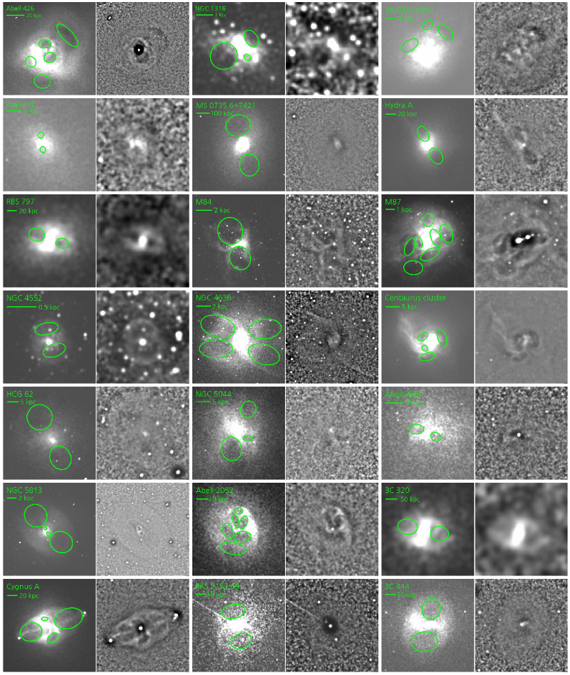
Figure 2.— Targets with cavity detections from raw images . Smoothed raw image (left) and unsharp masked image (right) are shown for each object. Detected cavities are denoted with green ellipse.

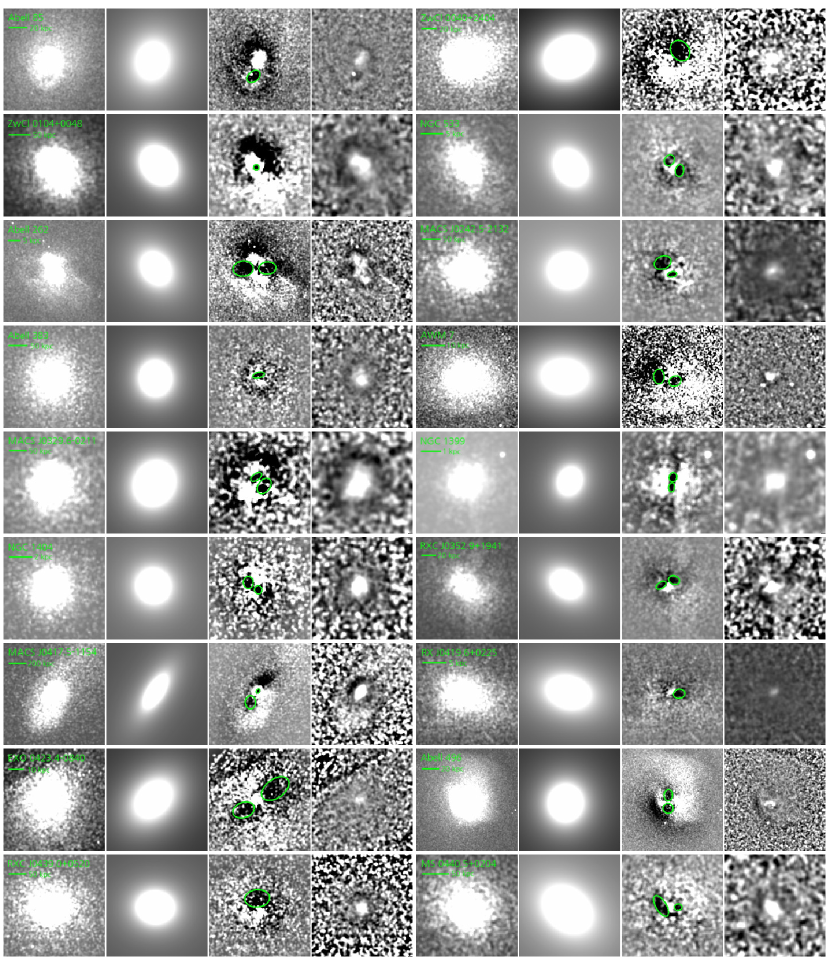
Figure 3.— Targets with cavity detections from the $\beta$-modeling. From left to right, smoothed raw image, $\beta$-model, residual image, and unsharp masked image are shown. Detected cavities are denoted with green ellipse.

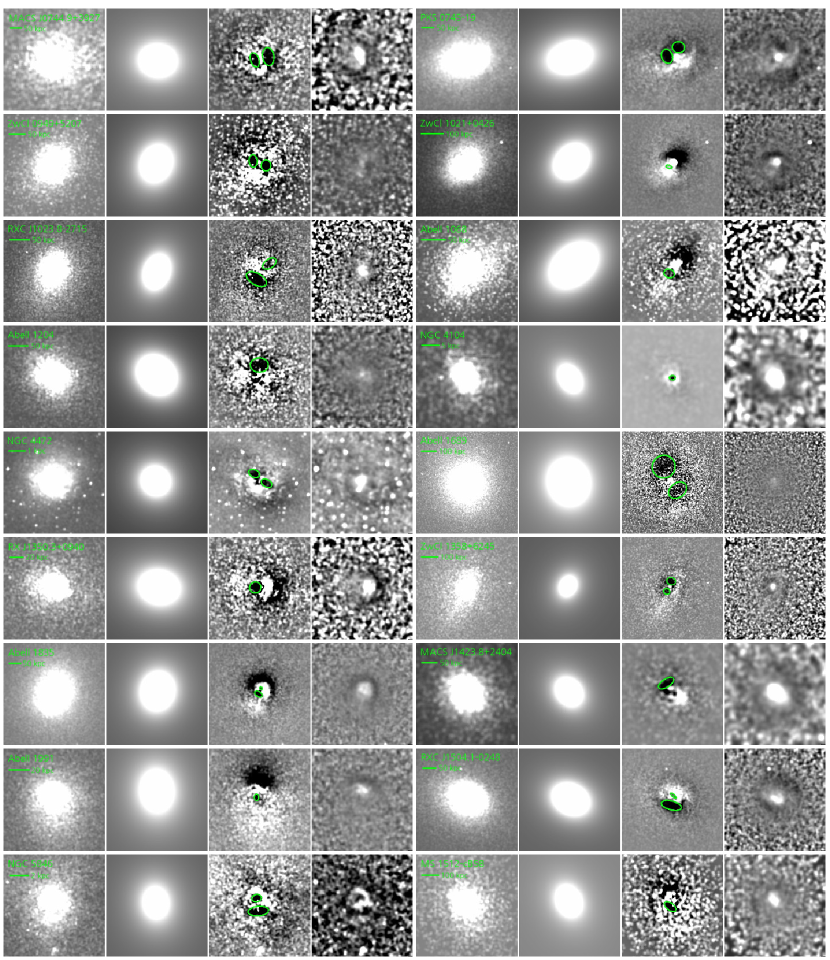
Figure 3.— continued

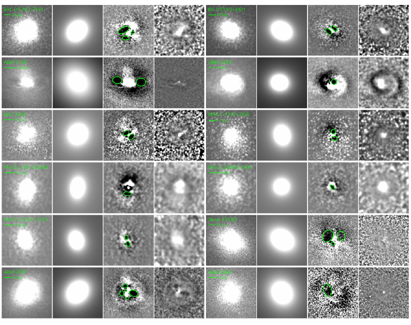
Figure 3.— continued

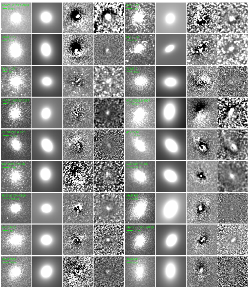
Figure 4.— Targets with non detections. From left to right, smoothed raw image, $\beta$-model, residual image, and unsharp masked image are shown.

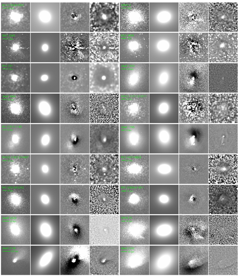
Figure 4.— continued

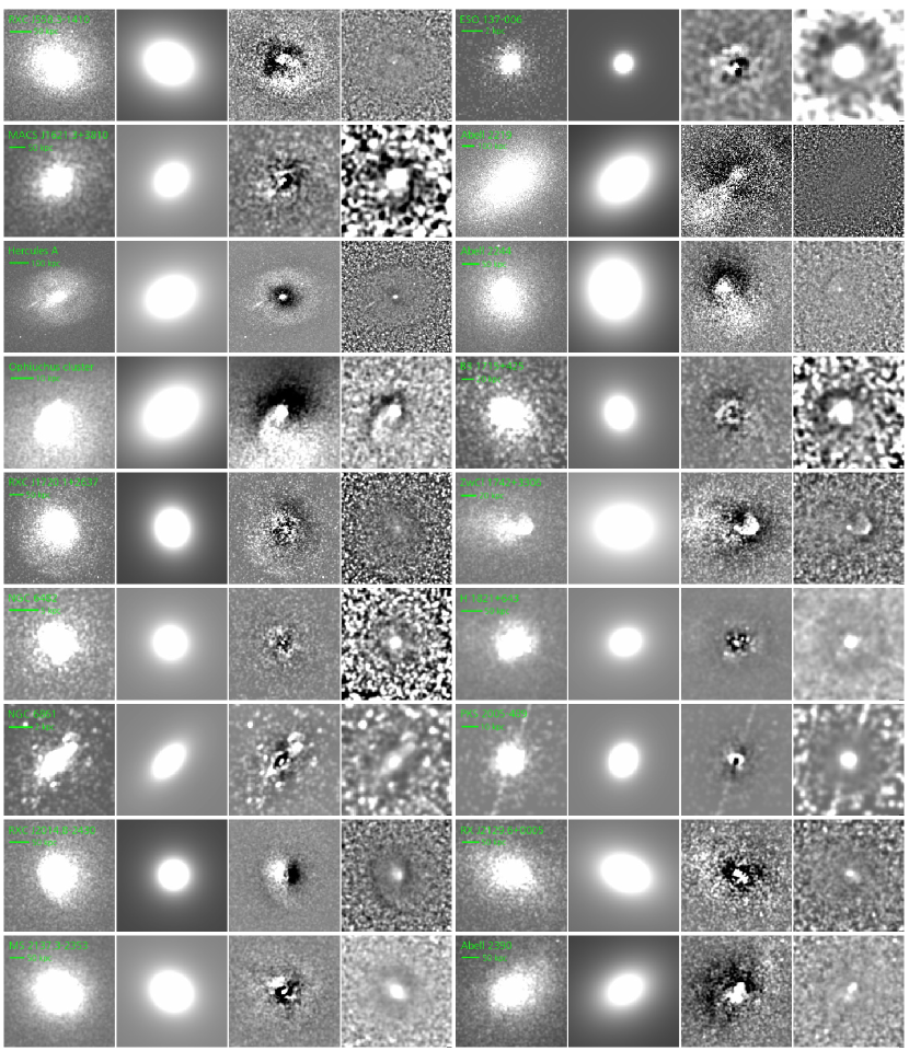
Figure 4.— continued

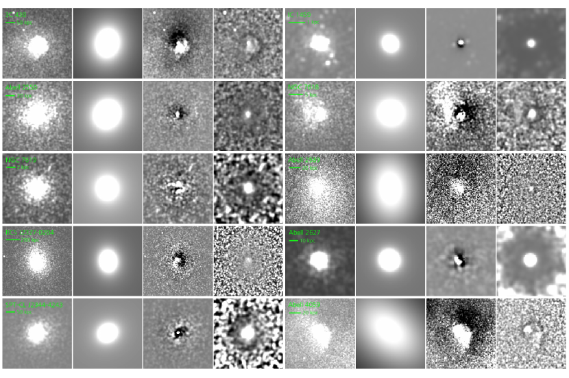
Figure 4.— continued

3.2. Cavity properties

We measured the properties of X-ray cavities, either directly detected from the raw X-ray images (for 21 targets) or detected from the $\beta$-model analysis (for 48 targets). Since the shape of X-ray cavities typically looks elliptical, we adopted an ellipse model to describe the morphology of X-ray cavities. Note that we tried to fit the shape of the individual X-ray cavities, but failed mainly due to the low photon counts. Thus, we simply overlapped an ellipse model to the raw and beta-model subtracted images, as similarly performed in the previous studies (Dong et al., 2010). Based on the ellipse model, we determined the size in the semimajor- and semiminor-axes of the X-ray cavities. Note that the size of cavities depends on the choice of the best ellipse model, hence the systematic uncertainty of the size can be significant (see Section 5.4 for more detailed discussion).

We also measured the distance between the cavity center (i.e., center of the ellipse) and the center of the diffuse X-ray emission, which is assumed to be the location of the point source. If a point source is not present, we adopted the peak position of diffuse X-ray emission as the center. We assumed 2 pixels as the measurement uncertainties of the cavity size and the distance. For three targets (ZwCl 0104+0048, NGC 4104, and MACS J2046.0-3430), the detected X-ray cavities are at the center of the diffuse X-ray emission. Perhaps, the radio jet direction is along the line-of-sight in these cases (see also Dong et al., 2010). In Table 2, we list the properties of X-ray cavities for individual targets.

3.3. False detections of X-ray cavities

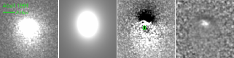
Figure 5.— Example of cold front targets, Abell 1991. Smoothed raw image (left), $\beta$-model (middle left), residual image after subtracting $\beta$-model (middle right), and unsharp masked image (right).

In our analysis, we find that asymmetric gas distributions (i.e., cold fronts) can produce false detections of X-ray cavities if we use a symmetric $\beta$-model. In Figure 5, we present such a case, Abell 1991, for which Dong et al. (2010) detected the presence of two cavities (see Figure 4. in Dong et al. 2010). The distribution of the diffuse emission is somewhat vertically asymmetric in the raw image with a sharp drop in the north and a shallow decrease in the south. As seen in the residual image after subtracting the $\beta$-model, we detected only one cavity in the south (middle right panel). There seems to be one more depression in the north but it may be still caused by the asymmetric X-ray gas distribution since the symmetric $\beta$-model can produce a false depression by over-subtracting the diffuse emission, respectively, in the north and south in the image. Thus, we conclude that the depression in the north may not be a real cavity, and that the fitting result may not be reliable for such targets with a strong asymmetric gas distribution. Nevertheless, as shown in the south, some targets show real X-ray cavities in the opposite part of sharp drop, where the diffuse emission is under-subtracted. Thus, the depression in the south is not likely a false detection.

Point sources (AGNs) in the center of diffuse emission may also lead to false detections. For example, in the presence of a strong point source at the center, the $\beta$-model tends to over-subtract diffuse emission around the point source, producing a false depression (see e.g., Abell 2029 and UGC12491 in Figure 4). For these cases, we did not classify them as real cavities. As presented in Figure 4, most of targets with no cavity detection present these two features, i.e., asymmetric distribution or over-subtraction around the point source. In these objects, it is not clear whether true cavities are present.

3.4. Gas temperature determination

To investigate the effect of the environments on X-ray cavities, we quantified the environments of each target in the sample. Since environments can be represented by various physical parameters, e.g., velocity dispersion of galaxies, X-ray gas temperature, and virial mass, we reviewed literatures for measured velocity dispersions and gas temperatures of each target. However, the reported values are often measured from different methods and incomplete for our sample.

To perform a uniform analysis and minimize systematic uncertainties, we directly measured the gas temperatures within $\rm 0.15\ R_{2500}$ based on the X-ray data. Since our targets cover a large redshift range (from 0.001 to 2.7), it is difficult to measure $\rm R_{2500}$ for all targets since, for example, the $\rm R_{2500}$ of low-redshift targets is far larger than the field of view (FOV) of Chandra images. After testing with various radii, we determined that $\rm 0.15\ R_{2500}$ is the optimal radius for the majority of targets in the sample. For several lower redshift targets, for which even $\rm 0.15\ R_{2500}$ is larger than the FOV, we adopted a smaller radius: $\rm 0.10\ R_{2500}$ for M84 and $\rm 0.05\ R_{2500}$ for NGC 4472, M87, NGC 4552, NGC 4636, and NGC 4649, respectively.

The $\rm 0.15\ R_{2500}$ was calculated from the temperature-radius relation (Equation 12 of Vikhlinin et al. 2006), using an initial temperature value. Since the $\rm R_{2500}$ varies depending on gas temperatures, we estimated $\rm 0.15\ R_{2500}$ by iterating radius determination until the estimated temperature becomes consistent within 10%. Note that the uncertainty of gas temperature is large since we calculate $\rm 0.15\ R_{2500}$ from gas temperature derived within $\rm 0.15\ R_{2500}$ while we used the temperature-radius relation derived for $\rm R_{2500}$.

The gas temperature derived from $\rm 0.15\ R_{2500}$ differs on average by 20% compared to that derived from $\rm R_{2500}$ (Vikhlinin et al., 2006). The method for gas temperature measurement is same as described in §2, except for the extraction radius. We estimated the uncertainties by combining 1 $\sigma$ fitting error and 20% systematic error to account for the temperature variation due to the adopted size of the aperture (i.e., $\rm 0.15\ R_{2500}$ vs. $\rm R_{2500}$). If a smaller radius (i.e., $<0.15\ R_{2500}$) was used for gas temperature measurements, we adopted 30% higher uncertainty, which is a maximum temperatures difference between $\rm 0.05\ R_{2500}$ $\rm 0.15\ R_{2500}$ (see Vikhlinin et al., 2006). If there is no reliable fitting error when $\chi^{2}$ is larger than 2, we adopted the maximum fitting error from other targets. Gas temperatures and HI column densities are presented in Table 1. Note that for individual sources, the uncertainty of the estimated temperature can be larger than 20-30% since $R_{2500}$ can be underestimated due to the degeneracy between temperature and radius.

Table 2Cavity properties

Object	$r_{a}$	$r_{b}$	Area	Distance
	(kpc)	(kpc)	(kpc2)	(kpc)
(1)	(2)	(3)	(4)	(5)
Abell 426	$16.4$	$6.0$	$307.5$	$29.6$
	$6.9$	$4.6$	$99.2$	$6.5$
	$6.9$	$5.6$	$120.5$	$10.2$
	$6.3$	$5.5$	$108.6$	$21.0$
	$9.1$	$7.3$	$208.1$	$35.7$
NGC 1316	$0.6$	$0.4$	$0.6$	$0.8$
	$0.8$	$0.8$	$2.0$	$1.2$
	$0.2$	$0.2$	$0.1$	$0.7$
2A 0335+096	$9.6$	$5.8$	$174.8$	$30.0$
	$6.3$	$4.3$	$83.9$	$28.4$
	$9.6$	$5.6$	$168.0$	$17.7$
Abell 478	$4.3$	$3.9$	$53.4$	$9.6$
	$4.2$	$4.1$	$54.6$	$11.3$
MS 0735.6+7421	$82.5$	$72.2$	$18714.7$	$167.4$
	$92.1$	$79.2$	$22921.3$	$139.5$
Hydra A	$16.4$	$11.2$	$574.6$	$23.8$
	$15.3$	$9.6$	$461.0$	$24.8$
RBS 797	$13.5$	$9.8$	$414.3$	$25.0$
	$16.2$	$13.3$	$677.8$	$30.1$
M84	$1.5$	$1.3$	$6.0$	$1.8$
	$1.7$	$1.6$	$8.3$	$2.1$
M87	$0.7$	$0.6$	$1.3$	$2.2$
	$1.0$	$0.6$	$2.1$	$2.4$
	$1.0$	$0.5$	$1.6$	$1.2$
	$0.6$	$0.4$	$0.7$	$0.7$
	$1.0$	$0.5$	$1.5$	$1.8$
	$1.1$	$0.5$	$1.9$	$1.6$
	$1.0$	$0.8$	$2.5$	$3.3$
NGC 4552	$0.2$	$0.1$	$0.1$	$0.2$
	$0.2$	$0.1$	$0.1$	$0.2$
NGC 4636	$2.2$	$1.4$	$9.5$	$3.8$
	$2.2$	$1.4$	$9.5$	$3.8$
	$2.4$	$1.5$	$11.3$	$3.7$
	$2.3$	$1.2$	$8.9$	$3.5$
Centaurus cluster	$2.9$	$1.5$	$13.5$	$3.5$
	$2.0$	$1.1$	$7.1$	$3.6$
	$1.2$	$0.9$	$3.3$	$3.6$
	$2.7$	$1.3$	$11.3$	$5.7$
HCG 62	$5.4$	$4.6$	$77.7$	$8.6$
	$5.7$	$5.6$	$98.9$	$11.7$
NGC 5044	$1.7$	$1.0$	$5.1$	$4.5$
	$4.1$	$3.4$	$43.6$	$6.5$
	$2.9$	$2.5$	$22.8$	$8.1$
Abell 3581	$3.0$	$2.4$	$23.2$	$5.4$
	$4.2$	$2.7$	$36.3$	$6.7$
NGC 5813	$1.0$	$0.7$	$2.2$	$1.6$
	$1.0$	$0.8$	$2.5$	$1.5$
	$4.8$	$4.5$	$68.4$	$7.6$
	$4.6$	$4.1$	$59.3$	$7.6$
Abell 2052	$4.3$	$3.0$	$40.5$	$13.9$
	$6.7$	$3.7$	$77.9$	$6.0$
	$5.7$	$3.0$	$54.4$	$7.5$
	$8.6$	$4.6$	$124.2$	$8.5$
	$7.1$	$4.2$	$93.5$	$11.0$
	$12.2$	$5.7$	$218.1$	$18.1$
3C 320	$16.3$	$12.9$	$660.5$	$28.5$
	$15.1$	$12.5$	$592.2$	$26.8$
Cygnus A	$21.1$	$17.5$	$1163.1$	$37.2$
	$11.7$	$7.6$	$279.0$	$24.3$
	$6.5$	$3.4$	$69.4$	$16.0$
	$28.1$	$19.2$	$1698.0$	$40.2$
PKS 2153-69	$11.6$	$7.1$	$259.7$	$14.8$
	$10.8$	$7.5$	$253.4$	$15.9$
3C 444	$61.4$	$46.6$	$9000.7$	$83.5$
	$50.8$	$43.0$	$6873.6$	$75.3$
Abell 85	$8.1$	$5.4$	$136.8$	$17.1$
ZwCl 0040+2404	$14.5$	$11.7$	$533.3$	$14.0$
ZwCl 0104+0048	$6.6$	$6.6$	$135.7$	$--$
NGC 533	$1.4$	$0.9$	$4.0$	$1.6$
	$1.3$	$1.1$	$4.4$	$1.8$
Abell 262	$3.7$	$2.5$	$29.4$	$3.7$
	$4.2$	$3.2$	$42.2$	$6.4$
MACS J0242.5-2132	$12.7$	$7.0$	$279.7$	$12.1$
MACS J0242.5-2132	$23.6$	$17.0$	$1261.2$	$28.7$
Abell 383	$16.0$	$7.4$	$371.0$	$8.2$
AWM 7	$2.7$	$2.1$	$17.7$	$3.9$
	$3.1$	$2.3$	$22.3$	$3.5$
MACS J0329.6-0211	$17.4$	$9.4$	$513.0$	$18.2$
	$24.2$	$16.4$	$1247.9$	$21.3$
NGC 1399	$0.2$	$0.2$	$0.1$	$0.2$
	$0.2$	$0.1$	$0.1$	$0.3$
NGC 1404	$0.5$	$0.4$	$0.7$	$0.7$
	$0.4$	$0.3$	$0.4$	$0.4$
RXC J0352.9+1941	$8.0$	$5.9$	$148.2$	$9.3$
	$7.9$	$4.3$	$107.4$	$10.8$
MACS J0417.5-1154	$13.8$	$9.4$	$406.8$	$10.9$
	$38.0$	$29.7$	$3543.8$	$76.4$
RX J0419.6+0225	$1.2$	$0.9$	$3.6$	$1.7$
EXO 0423.4-0840	$9.9$	$5.9$	$184.4$	$14.0$
	$7.1$	$4.8$	$106.5$	$10.4$
Abell 496	$6.5$	$4.7$	$97.1$	$8.8$
	$5.9$	$5.6$	$103.2$	$6.3$
RXC J0439.0+0520	$35.6$	$25.0$	$2796.2$	$25.3$
MS 0440.5+0204	$7.2$	$5.9$	$133.1$	$15.7$
	$21.8$	$9.5$	$650.7$	$17.7$
MACS J0744.9+3927	$45.3$	$28.6$	$4062.3$	$43.6$
	$37.1$	$21.0$	$2439.5$	$28.6$
PKS 0745-19	$9.9$	$8.8$	$273.5$	$18.4$
	$11.6$	$8.5$	$310.7$	$9.3$
ZwCl 0949+5207	$16.1$	$13.9$	$699.6$	$21.9$
	$18.5$	$12.0$	$696.1$	$18.1$
ZwCl 1021+0426	$13.5$	$7.1$	$300.0$	$33.0$
RXC J1023.8-2715	$52.9$	$27.8$	$4623.6$	$38.5$
	$36.6$	$21.2$	$2441.9$	$61.4$
Abell 1068	$10.9$	$8.7$	$299.3$	$22.7$
Abell 1204	$22.1$	$17.4$	$1212.4$	$23.8$
NGC 4104	$0.9$	$0.6$	$1.7$	$--$
NGC 4472	$0.3$	$0.2$	$0.2$	$0.5$
	$0.3$	$0.2$	$0.2$	$0.4$
Abell 1689	$79.9$	$71.1$	$17843.4$	$109.6$
	$63.9$	$46.4$	$9314.9$	$67.7$
RX J1350.3+0940	$8.1$	$7.8$	$199.3$	$9.1$
ZwCl 1358+6245	$31.4$	$24.9$	$2451.7$	$33.4$
	$22.3$	$20.3$	$1420.4$	$45.5$
Abell 1835	$16.9$	$9.9$	$527.8$	$14.3$
	$5.8$	$5.6$	$102.3$	$11.0$
MACS J1423.8+2404	$27.1$	$12.7$	$1082.3$	$36.1$
Abell 1991	$4.5$	$3.3$	$46.3$	$8.3$
RXC J1504.1-0248	$13.6$	$4.5$	$191.6$	$11.9$
	$36.6$	$15.6$	$1789.8$	$23.5$
NGC 5846	$1.1$	$0.5$	$1.7$	$0.8$
	$0.5$	$0.4$	$0.6$	$0.5$
MS 1512-cB58	$43.4$	$18.4$	$2507.1$	$73.0$
RXC J1524.2-3154	$19.5$	$8.9$	$545.1$	$13.9$
	$5.4$	$4.1$	$70.3$	$16.3$
	$11.1$	$6.4$	$223.1$	$23.3$
RX J1532.9+3021	$31.3$	$16.8$	$1653.4$	$32.7$
	$29.9$	$14.5$	$1359.1$	$22.7$
Abell 2199	$8.0$	$6.2$	$155.0$	$19.7$
	$8.6$	$7.0$	$187.8$	$22.7$
Abell 2204	$10.0$	$9.4$	$295.2$	$13.0$
NGC 6338	$3.8$	$2.3$	$27.1$	$3.2$
	$3.7$	$2.5$	$28.5$	$4.3$
MACS J1720.3+3536	$17.6$	$16.8$	$929.8$	$25.4$
	$20.7$	$16.8$	$1089.1$	$27.5$
MACS J1931.8-2634	$19.6$	$9.0$	$551.3$	$30.3$
MACS J2046.0-3430	$14.4$	$7.2$	$328.2$	$--$
MACS J2229.7-2755	$8.8$	$7.2$	$199.5$	$12.3$
	$11.8$	$9.0$	$333.7$	$18.5$
Sersic 159-03	$15.3$	$12.3$	$592.9$	$29.5$
	$6.2$	$4.4$	$86.4$	$13.5$
	$20.5$	$16.3$	$1052.7$	$21.5$
Abell 2597	$7.3$	$6.0$	$138.9$	$21.7$
	$3.1$	$2.9$	$28.7$	$9.4$
	$8.7$	$6.6$	$179.6$	$21.6$
	$5.1$	$3.0$	$48.2$	$20.6$
	$14.0$	$9.6$	$422.6$	$17.4$
Abell 2626	$19.9$	$12.4$	$775.5$	$18.1$
Note – Col. (1): Object name. Col. (2): Semimajor axis. Col. (3):
Semiminor axis. Col. (4): Area of X-ray cavity. Col. (5): Distance
from X-ray gas emission center to X-ray cavity center. The border
divides the detected X-ray cavities from raw images (upper) and beta
-model subtracted images (lower).

4. Result

4.1. Cavity detection

Using the raw images and applying the $\beta$-model, we detected 148 cavities from 69 targets. Out of the 133 targets in our sample with sufficient X-ray photons, $\sim$ 52% shows cavities. Among them, 18, 38, and 13 targets show one, two and more than two cavities, respectively. In general, two cavities are detected as a pair on opposite sides of the center, except for a few cases. Since X-ray cavities are believed to be formed by a radio jet, two bi-symmetric X-ray cavities are expected. However, the presence of more than two cavities in many targets may imply that there were multiple radio events in the past. In the case of more than 2 cavities, 4 targets show one pair and one additional cavity (1, NGC 1316) while the other 9 targets show various geometry: collinear two pairs (e.g., NGC 5813), two pairs with different direction (2, e.g., NGC 4636 & Cygnus A), or a complicated structure (6, e.g., Abell 426 & M87).

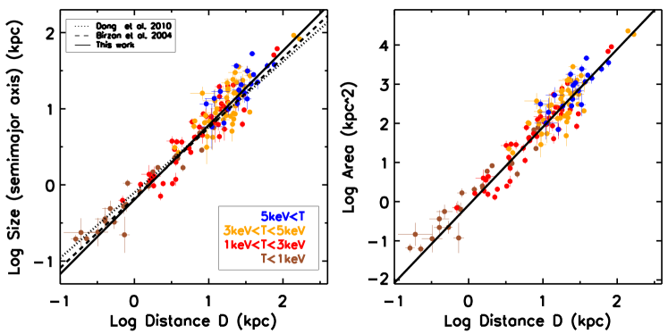
Figure 6.— Comparison between our result and previous results. Semimajor axis and distance comparison (left), and area and distance comparison (right).

4.2. Cavity properties comparison

To investigate relations between cavity properties, we compared the cavity size in the semimajor axis (a), distance from the X-ray center (D), and area as shown in Figure 6, using the ”FITEXY” method (Tremaine et al., 2002; Park et al., 2012). To calculate uncertainties, we performed Monte Carlo simulations with 10,000 mock datasets by randomizing the error, and adopted the standard deviation as the uncertainty of the fitting results.

Over the large dynamic range covered by our sample, we confirm a linear correlation of the cavity size with the distance from the X-ray center,

$${\rm log}\ a=(0.97\pm 0.02)\ {\rm log}\ D-0.15\pm 0.02,$$ (1)

as previous studies reported (Bîrzan et al., 2004; Dong et al., 2010). There are several explanations to understand this correlation in terms of cavity evolution such as buoyancy or momentum from AGN jet. By testing various models, Diehl et al. (2008) showed that magnetically-dominated cavities can be well explained by current-dominated magnetohydrodynamic jet models (Li et al., 2006; Nakamura et al., 2006, 2007)).

Since the cavity shape is generally elliptical, cavity area may better represent the cavity property than the size in the semimajor- or semiminor- axes. In addition, to estimate the total energy emitted from a radio jet, the volume of cavities is required based on additional assumptions (i.e., cavity shape). Instead, cavity area can be measured from the projected image and compared to the distance. As shown in right panel of Figure 6, we find a similar correlation between the cavity area and the distance from the center

$${\rm log}\ Area=(1.94\pm 0.04)\ {\rm log}\ D+0.02\pm 0.05.$$ (2)

The scatter of the area-distance relation is similar to that of the size-distance relation (0.155$\pm$0.010 dex and 0.163$\pm$0.011 dex, respectively, in distance unit). For the rest of paper, we will use the area as the representative of the cavity size. In Figure 6, gas temperatures are denoted with different colors. Of interest, it seems that high temperature systems tend to have larger cavities. However, the cavity size correlates with the distance regardless of gas temperature, suggesting that the formation and evolution of the X-ray cavities has little dependence on environment.

4.3. X-ray cavity and gas temperature

To investigate the environmental effects on X-ray cavities, we first checked the fraction of X-ray cavity detection as a function of X-ray gas temperatures in Figure 7. At each temperature bin, the number of total targets and the number of targets with cavity detection are represented, respectively, with the unfilled- and filled-histogram. The detection rate of X-ray cavities is on average 49% while the rate varies slightly in individual temperature bins. We do not find a significant change of the detection rate except for the very high temperature bins that contain small number of targets, suggesting that no strong environmental effects on the presence of X-ray cavities.

In contrast, there appears to be a trend between cavity size and environments. By comparing cavity sizes to gas temperatures (Figure 8), we find that the cavity size increases with gas temperatures. Since many targets at given gas temperature have multiple cavities with various sizes, the relation between the cavity size and gas temperature is not strong. Nonetheless, there is a clear trend between them, suggesting that more massive systems possess larger size cavities. However, to confirm the correlation, we should look at the selection effect carefully, which will be discussed in detail in §5.1.

Figure 7.— X-ray cavity detection on temperature distribution. Total number (unfilled) and X-ray cavity detection number (filled) are represented.

Figure 8.— Cavity size as a function of the gas temperature of each targets.

5. Discussion

5.1. Dependence on environments

Previous studies reported that the X-ray cavity detection rate is $\sim$2/3 for cool-core clusters (14 out of 20; Dunn & Fabian, 2006), $\sim$1/2 for galaxy groups (26 out of 51; Dong et al., 2010), and $\sim$1/4 for elliptical galaxies (24 out of 104; Nulsen et al., 2009). At face value these results seem to suggest that the detection rate of X-ray cavity increases with galaxy density, indicating environment effects on the formation of X-ray cavities.

As pointed in §2, however, consistent criteria for sample selection and uniform analysis is required to constrain the detection rate and environment effect. By investigating the targets in the previous studies, we find that many targets, for which X-ray cavities were detected, do not have sufficient X-ray photons. For example, 17 targets of Dong et al. (2010) satisfy our sample selection criteria while the other 38 targets have insufficient photon counts. Among those 17 targets, we found cavities in 11 targets while Dong et al. (2010) detected cavities in 14 targets. Comparing with the results of Dunn & Fabian (2006), we used all 20 objects in their sample and detected cavities in 16 objects. While Dunn & Fabian (2006) also detected cavities in 16 targets, they did not find cavities in the same 16 targets we did. We found X-ray cavities in Abell 496, Abell 2204, PKS 0745-191, and AWM7, however, Dunn & Fabian (2006) did not. It may be partly due to the fact that Dunn & Fabian (2006) used single exposures per target, without combining all available exposures and that they did not perform $\beta$-modeling and unsharp masking analysis. On the other hand, Dunn & Fabian (2006) reported X-ray cavities in Abell 1795, Abell 2029, Abell 4059, and MKW 3s, while we classified these target as non-detections since they show over-subtraction in our analysis. These examples demonstrate the difficulties of direct comparison among various studies in the literature. We provide more detailed comparison of our work to others in §5.4.

In contrast, our results suggest that the cavity detection rate does not show significant dependence on gas temperatures (see Figure 7), indicating that the formation and evolution of the X-ray cavities may be driven by the central engine (i.e., AGN) and affected by the physical conditions at the center (i.e., gas density) rather than the global properties (i.e., environments).

We showed that larger X-ray cavities tend to be detected in the higher gas temperature systems. Since the cavity grows in size and moves away from the center, as indicated by the size-distance relationship, we expect to see small cavities close to the center even in high gas temperature systems. The lack of small cavities in high gas temperature systems may reflect selection effects. To investigate the effect, we compared the cavity size and gas temperature as a function of redshift (Figure 9), finding that systems with high gas temperature tend to be more distant since more massive and more luminous systems with high gas temperature are rarer. Also, we tend to detect larger cavities at higher redshift as shown in Figure 9. This trend can be due to the limited spatial resolution of the Chandra data. Since it is difficult to identify a cavity with a size smaller than $\sim$1″with the $Chandra$ PSF, we could not detect small size cavities at high redshift. To illustrate this, we denoted the detection limit for a cavity with a 1″ radius size as a function of redshift with a solid line in Figure 9. The distribution of the detected cavities over the redshift range is consistent with the detection limit, indicating that the lack of small cavities at high redshift is due to the fixed spatial resolution in Chandra images.

On the other hand, we tend to detect no large cavities in the systems with lower gas temperature since the size of the diffuse X-ray emitting region is intrinsically small. Since the cavities are detected as a form of depression as embedded in the diffuse X-ray gas, the size of X-ray emitting region is the maximum limit of the cavity size. In Figure 10, we present the size of the X-ray halo with a grey line, which represents $\rm R_{2500}$ as a function of gas temperature while the thickness represents the range of $\rm R_{2500}$ at the redshift range 0.001¡z¡0.7, which is relevant for all targets in the sample except for one target, MS 1512-cB58 at z = 2.723. This figure demonstrates the growth limit of X-ray cavities. For example, 3C 444 ($\rm{\log\ (D/1kpc)\sim 1.8}$) and MS 0735.6+7421 ($\rm{\log\ (D/1kpc)\sim 2.2}$) contain relatively large cavities, which are close to the growth limit and detected at the edge of the X-ray distribution. There are other cavities detected at the edge of the X-ray distribution (e.g., M84 and NGC 4636). However, these target have much shallower X-ray images, hence, the size of the observed X-ray distribution is much smaller than $\rm R_{2500}$.

In Figure 11, we demonstrate the two forbidden areas in the size-temperature plane with the growth limit and the spatial resolution limit. Intrinsically the cavity size can not be larger than the X-ray emitting region of individual targets, confining the detected cavities below the growth limit, while Chandra image resolution does not allow us to observationally detect small cavities below the spatial resolution limit.

Figure 9.— Relation between gas temperature and redshift (top) and relation between area of X-ray cavities and redshift (bottom). Solid line in the bottom panel shows the area of a circle with a radius of 1″as a function of the redshift.

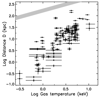
Figure 10.— Distribution of gas temperature and cavity distance from the center. Thin gray region indicates $\rm R_{2500}$ calculated from gas temperature for the redshift range (0.001¡z¡0.7).

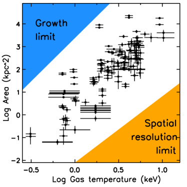
Figure 11.— Same figure as Figure 8. Orange and blue areas mean spatial resolution limit area and growth limit area. Black color shows the measurement from individual cavity.

5.2. Non-detection of X-ray cavity

While we detected X-ray cavities from 69 out of 133 targets, we did not find any clear evidence for X-ray cavities in the other 64 targets (see §4). Since the majority of non-detected targets have asymmetric distributions or over-subtraction issues, it is difficult to confirm the presence of cavities in these objects. This is the limitation of this work since we relied on symmetric $\beta$-modeling. The results from the $\beta$-modeling often present over-subtraction regions, which were classified as non-detections. For these targets, additional data such as radio can be an aid to reveal the true nature of diffuse X-ray emission. For example, Hodges-Kluck et al. (2010a, b) confirmed the presence of cavities by combining X-ray and radio data.

Another possible reason for non-detection is relatively weak X-ray depression. Previous work reported that cavity detectability strongly depends on the size and distance from the center, suggesting that large cavities with smaller distance can be detected easily (Enßlin & Heinz, 2002; Brüggen et al., 2009; Dong et al., 2010). In other words, we tend to not detect small cavities far from the central region. In addition, Enßlin & Heinz (2002) showed that detectability also relies on the inclination angle of a cavity with respect to the plane of sky, showing that cavity depression is maximized when the inclination angle is zero. For these reasons, it is likely that we may have missed some cavities. These effects act as selection effects for our cavity detection and the observed size-distance relation presented in Figure 6.

We consider two additional scenarios for systems with no cavity detections. One scenario is that no X-ray cavity is present due to the lack of AGN or jets. If there are no radio jets or the radio jets are too weak to push the hot X-ray gas, cavities may not form. As a possible AGN indicator, we investigate the presence of an X-ray point source at the center of each object. We found a central X-ray point source for 33 out of 69 cavity-detected targets (48%) and 33 out of 64 targets with no cavity detection (52%), respectively, suggesting that X-ray AGN fraction is similar between targets with/without cavities. In the case of the cavity-detected targets without X-ray AGN, it is possible that AGN is currently very weak or inactive while the black hole was active in the past. In the case of no cavity targets with X-ray AGNs, the AGN may not have strong jets to form cavities, or cavities are present, but not detected due to the detection issues (i.e., asymmetric distribution or over-subtraction). A detailed investigation of the relationship between AGN and the presence of cavities is beyond the scope of our current work.

Another possibility is that the radio jet was just launched or launched a long time ago. If the radio jet is just launched, cavities may be too small to resolve in the X-ray images. If the radio jet launched a long time ago, the X-ray cavities may have already moved beyond the edge of the diffuse X-ray emission (see §5.1)

To check this scenario, one can use multi-frequencies radio data. In detecting X-ray cavities directly, high-frequency data with high resolution could reveal small X-ray cavities. However, due to the energy loss through synchrotron emission, there could be no emission at high-frequency if the jet was launched a long time ago. In that case, low-frequency observations might reveal extended features (e.g., Gitti et al., 2010; Giacintucci et al., 2011). With the combination of multi-frequency radio data, one can check for the presence of radio jets at small and large scales. If there is no radio jet, it could mean there was no AGN activity and thus no cavities as well. On the other hand, if there is the evidence of radio jets at small- or large- scales, it could be good evidence to confirm the second scenario. Furthermore, if the radio image shows multiple jets, it enables us to investigate the duty cycle of AGN activity (e.g., Randall et al., 2011; Chon et al., 2012). In means that we can study in detail the period of AGN feedback duty cycle. However, the current lack of multi-frequency radio data for our targets makes such a study not possible in the current paper.

We note that a scaling relation between jet power derived from the cavities and radio luminosity has been found (Bîrzan et al., 2004, 2008; Cavagnolo et al., 2010; O’Sullivan et al., 2011a). In other words, the jet power can be estimated based on radio luminosity and used to predict the presence of X-ray cavities. Thus, this may be another way to infer the existence of cavities when they can not be directly detected in X-ray images.

5.3. The shape of X-ray cavities

In Figure 12, we present a distribution of orientation angle of the cavities with respect to the center (or jet direction). We define the orientation angle 0 degree if the cavity is radially elongated (along with the jet direction; e.g., Cygnus A and Hydra A) while 90 degree means that the cavity is elongated perpendicular to the jet direction (e.g., NGC 4552 and HCG 62). Here, we only take the targets with a/b ratio over 1.1 or under 0.9 to avoid a systematic uncertainty from circular shape cavity. We find a bimodal distribution that cavities are elongated either parallel to the jet direction or perpendicular to the jet direction, suggesting no significant trend with respect to the jet direction. Note that since we did not fit the cavity with an ellipse model, and determined a representative model by visual inspection, the uncertainty of the direction of the elongation is relatively large.

While various simulation results showed different orientations (Sijacki & Springel, 2006; Brüggen et al., 2007; Sijacki et al., 2007; Dubois et al., 2010; Gaspari et al., 2011; Li & Bryan, 2014), a recent study by Guo (2015) investigated the orientation of cavities with various input physical parameters, suggesting that radial elongation increases with jet density, velocity, and duration while it decreases with jet energy density and radius, implying that the morphology of the cavities is closely related to the jet properties.

Figure 12.— Distribution of the orientation angle of X-ray cavities. 0 degree indicates radial elongation while 90 degree means that major axis is perpendicular to the jet direction.

5.4. Comparison to previous works

In this section, we compare our cavity detections with previous studies. First, we used the initial sample of $\sim$800 targets, for which we obtained evidence for diffuse X-ray emission and performed a detailed X-ray count analysis (see §2), to find whether X-ray cavities were previously detected by other studies. By searching a number of papers cited for each target, we find that 116 out of $\sim$800 targets were reported to possess X-ray cavities in the literature.

Among these 116 targets, 69 targets have Chandra images with sufficient X-ray photons (i.e., larger than 4 counts per pixel at the 6-7 pixel annulus; see §2) while the X-ray image of the other 47 targets does not have sufficient photons, hence we did not perform the detailed analysis for these targets. The X-ray cavities of these 69 targets were identified by a number of works (e.g., Bîrzan et al., 2004; Dunn et al., 2005; Dunn & Fabian, 2006; Rafferty et al., 2006; Diehl et al., 2008; Cavagnolo et al., 2010; Giacintucci et al., 2011; Bîrzan et al., 2012; Hlavacek-Larrondo et al., 2012; Russell et al., 2013; Panagoulia et al., 2014). When we compare them with our work, we find that we independently detected cavities from 47 of these targets. We did not detect X-ray cavities in 22 other targets that were previously claimed to contain X-ray cavities. Since over-subtraction is shown in these targets, we classified them as no-cavity detections (see Figure 4). For these more complex objects, additional information such as radio flux and morphology may help to confirm the existence of the cavities. Note that the presence of X-ray cavities have been confirmed using radio data (e.g., IRAS 09104+4109, O’Sullivan et al. 2012; NGC 4261, O’Sullivan et al. 2011b; Abell 2029, Clarke et al. 2004; and Hercules A, Nulsen et al. 2005a). However, to be consistent with other over-subtraction targets, we left them as no-cavity detections based on X-ray data only.

For the other 47 targets out of the 116 objects, X-ray cavities were also reported in the literature (e.g., Rafferty et al., 2006; Cavagnolo et al., 2010; Dong et al., 2010; Hodges-Kluck et al., 2010a, b; Lal et al., 2010; Machacek et al., 2010; O’Sullivan et al., 2010; Bîrzan et al., 2012; Panagoulia et al., 2014; Hlavacek-Larrondo et al., 2015). In our analysis, however, these targets were excluded from the detailed $\beta$-modeling and further analysis since the X-ray images did not satisfy the criterion of having sufficient photons. For example, Panagoulia et al. (2014) investigated a sample of 49 objects, finding X-ray cavities from 30 targets, while only 28 targets among their 49 objects were included in our analysis based on the photon count criterion. As described in §2, we note that photon count is the most important parameter for detecting X-ray cavities in our analysis, thus deeper X-ray images are required for confirming cavities in these targets.

In our analysis of the total sample of 133 targets with sufficient X-ray photons, we detected X-ray cavities for 69 objects. While 47 objects among them were previously reported to have X-ray cavities, we found new X-ray cavities for 22 additional objects for the first time. In particular, 5 targets out of these 22 objects were studied by previous works, however, no X-ray cavities were identified. They are namely, AWM 7 (Dunn & Fabian, 2006; Bîrzan et al., 2012), EXO 0423.4-0840, RXC J1504.1-0248 (Bîrzan et al., 2012), and Abell 2626 (Panagoulia et al., 2014). One of the reasons why we were able to detect cavities in these objects is that we used deeper X-ray images by combining individual exposures, which is the case for 4 targets. For the other object, RXCJ 1504.1-0248, although the same X-ray data were used for both our and previous works, we used the $\beta$-modeling while the previous works used raw images and unsharp masking method (except for Dong et al. 2010). Thus, the difference of the depth of the X-ray images and the analysis method seems to explain the discrepancy.

We find that the number of detected cavities for a given target is sometimes different from that of previous studies, presumably due to the use of different analysis methods. For example, we detected three cavities in NGC 5044 and NGC 1316, respectively, while David et al. (2009) detected four cavities in NGC 5044 and Lanz et al. (2010) found only one cavity in NGC 1316. Forman et al. (2007) and Wise et al. (2007) also detected cavities from Hydra A and M87, respectively, but the number of detected cavities in their studies is different from that of this work. In those studies, radio data were additionally used to confirm the presence of cavities, that were not classified as cavities with the X-ray data alone in our study, suggesting that our analysis and measurements of cavity properties are limited. A more statistical investigation of the various X-ray studies for cavities is beyond the scope of this paper.

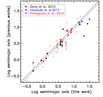
Figure 13.— Comparison of cavity sizes. Black, blue and red points indicate the measurements by Dong et al. (2010); Hlavacek-Larrondo et al. (2012); Panagoulia et al. (2014), respectively. Open and filled circle show cavity detected from raw image and based on the $\beta$-modeling. Dotted and dashed lines denote one-to-one relationship and mean offset by 0.07 dex. The values show semi-major axis.

We have compared the properties of the cavities detected in our study with those in the literature for a consistency check. For this exercise, we used three studies (Dong et al., 2010; Hlavacek-Larrondo et al., 2012; Panagoulia et al., 2014) since they provide cavity size as well as X-ray images, enabling us to crossmatch the cavities detected in our study. We found 44 cavities in 24 targets that are common to these other studies. Among these targets, 9 cavities are detected by both Dong et al. (2010) and Panagoulia et al. (2014). By comparing the size of these 44 cavities in Figure 13, we find that the cavity size is similar to that of previous works within 0.07 dex. Compared to the scatter (0.17 dex), our measurements show a good agreement with those in the previous work. When we divided the cavities into two categories: cavities detected from raw images (open) and based on the $\beta$-modeling (filled), we do not find any significant difference in comparison. The solid vertical lines between black and red symbols show the nine overlappng cavities between Dong et al. (2010) and Panagoulia et al. (2014). The mean difference of this subsample between two previous works is 0.06 dex, implying negligible difference. Note that the sample of Hlavacek-Larrondo et al. (2012) seems to show the largest offset (0.15 dex) among the three works, while the difference is still smaller than the overall scatter (0.17 dex), suggesting that cavity size measurements are relatively consistent among various works.

6. Summary

Using all available X-ray data ($\sim$ 5500 exposures) from the Chandra archive, we selected a sample of 133 targets with sufficient X-ray photon counts to search for X-ray cavities. Based on our consistent analysis we presented X-ray cavities detections for 69 targets over a large dynamic range from isolated galaxy to massive galaxy clusters. We summarize the main results as follows.

$\bullet$ Using various detection strategies (raw image, $\beta$-modeling, unsharp masking method), we found 148 X-ray cavity in 69 targets out of a total sample of 133 objects, which is $\sim$ 52% detection rate. The detection rates of X-ray cavities are similar among individual galaxies, galaxy groups, and galaxy clusters. Most targets have more than two cavities, suggesting multiple AGN outbursts.

$\bullet$ We confirmed the cavity size-distance relation over a large dynamic range and environments. We propose that the area of a cavity is a useful parameter to represent the physical size of cavities.

$\bullet$ We found little dependence of the cavity properties on environment. This may indicate that X-ray cavities form universally and are not driven by global properties of the system, but determined by the properties of AGN and its radio jets.

$\bullet$ The apparent relation between X-ray cavity size and X-ray gas temperature suffers from selection effects due to the observational limit of the spatial resolution of Chandra images as well as the intrinsic limit of the size of X-ray emitting region, particularly for low gas temperature systems.

In this work, we found that X-ray cavities have similar properties in galaxies, groups and clusters and therefore conclude that their formation is independent of environment. We also suggest that AGN feedback occurs periodically based on the high fraction of X-ray cavity detection and multiple pairs of X-ray cavities. Using our sample, follow-up studies can investigate X-ray cavities comprehensively as a probe of AGN feedback.

References

- Bae & Woo (2014) Bae, H.-J., & Woo, J.-H. 2014, ApJ, 795, 30
- Barbosa et al. (2009) Barbosa, F. K. B., Storchi-Bergmann, T., Cid Fernandes, R., Winge, C., & Schmitt, H. 2009, MNRAS, 396, 2
- Bîrzan et al. (2008) Bîrzan, L., McNamara, B. R., Nulsen, P. E. J., Carilli, C. L., & Wise, M. W. 2008, ApJ, 686, 859
- Bîrzan et al. (2004) Bîrzan, L., Rafferty, D. A., McNamara, B. R., Wise, M. W., & Nulsen, P. E. J. 2004, ApJ, 607, 800
- Bîrzan et al. (2012) Bîrzan, L., Rafferty, D. A., Nulsen, P. E. J., et al. 2012, MNRAS, 427, 3468
- Blanton et al. (2011) Blanton, E. L., Randall, S. W., Clarke, T. E., et al. 2011, ApJ, 737, 99
- Bogdán & Gilfanov (2008) Bogdán, Á., & Gilfanov, M. 2008, MNRAS, 388, 56
- Boroson (2005) Boroson, T. 2005, AJ, 130, 381
- Bower et al. (2006) Bower, R. G., Benson, A. J., Malbon, R., et al. 2006, MNRAS, 370, 645
- Brüggen et al. (2007) Brüggen, M., Heinz, S., Roediger, E., Ruszkowski, M., & Simionescu, A. 2007, MNRAS, 380, L67
- Brüggen et al. (2009) Brüggen, M., Scannapieco, E., & Heinz, S. 2009, MNRAS, 395, 2210
- Cavagnolo et al. (2010) Cavagnolo, K. W., McNamara, B. R., Nulsen, P. E. J., et al. 2010, ApJ, 720, 1066
- Cavaliere & Fusco-Femiano (1976) Cavaliere, A., & Fusco-Femiano, R. 1976, A&A, 49, 137
- Chon et al. (2012) Chon, G., Böhringer, H., Krause, M., & Trümper, J. 2012, A&A, 545, L3
- Churazov et al. (2001) Churazov, E., Brüggen, M., Kaiser, C. R., Böhringer, H., & Forman, W. 2001, ApJ, 554, 261
- Ciotti et al. (2010) Ciotti, L., Ostriker, J. P., & Proga, D. 2010, ApJ, 717, 708
- Clarke et al. (2004) Clarke, T. E., Blanton, E. L., & Sarazin, C. L. 2004, ApJ, 616, 178
- Crenshaw et al. (2003) Crenshaw, D. M., Kraemer, S. B., & George, I. M. 2003, ARA&A, 41, 117
- Croston et al. (2008) Croston, J. H., Hardcastle, M. J., Birkinshaw, M., Worrall, D. M., & Laing, R. A. 2008, MNRAS, 386, 1709
- Croton et al. (2006) Croton, D. J., Springel, V., White, S. D. M., et al. 2006, MNRAS, 365, 11
- David et al. (2009) David, L. P., Jones, C., Forman, W., et al. 2009, ApJ, 705, 624
- Di Matteo et al. (2005) Di Matteo, T., Springel, V., & Hernquist, L. 2005, Nature, 433, 604
- Dickey & Lockman (1990) Dickey, J. M., & Lockman, F. J. 1990, ARA&A, 28, 215
- Diehl et al. (2008) Diehl, S., Li, H., Fryer, C. L., & Rafferty, D. 2008, ApJ, 687, 173
- Dong et al. (2010) Dong, R., Rasmussen, J., & Mulchaey, J. S. 2010, ApJ, 712, 883
- Dubois et al. (2010) Dubois, Y., Devriendt, J., Slyz, A., & Teyssier, R. 2010, MNRAS, 409, 985
- Dunn & Fabian (2006) Dunn, R. J. H., & Fabian, A. C. 2006, MNRAS, 373, 959
- Dunn et al. (2005) Dunn, R. J. H., Fabian, A. C., & Taylor, G. B. 2005, MNRAS, 364, 1343
- Enßlin & Heinz (2002) Enßlin, T. A., & Heinz, S. 2002, A&A, 384, L27
- Fabian (1994) Fabian, A. C. 1994, ARA&A, 32, 277
- Fabian (2012) —. 2012, ARA&A, 50, 455
- Fabian et al. (2002) Fabian, A. C., Celotti, A., Blundell, K. M., Kassim, N. E., & Perley, R. A. 2002, MNRAS, 331, 369
- Fabian et al. (2006) Fabian, A. C., Sanders, J. S., Taylor, G. B., et al. 2006, MNRAS, 366, 417
- Fabian et al. (2000) Fabian, A. C., Sanders, J. S., Ettori, S., et al. 2000, MNRAS, 318, L65
- Ferrarese & Merritt (2000) Ferrarese, L., & Merritt, D. 2000, ApJ, 539, L9
- Forman et al. (2007) Forman, W., Jones, C., Churazov, E., et al. 2007, ApJ, 665, 1057
- Gaibler et al. (2012) Gaibler, V., Khochfar, S., Krause, M., & Silk, J. 2012, MNRAS, 425, 438
- Ganguly et al. (2007) Ganguly, R., Brotherton, M. S., Cales, S., et al. 2007, ApJ, 665, 990
- Gaspari et al. (2012) Gaspari, M., Brighenti, F., & Temi, P. 2012, MNRAS, 424, 190
- Gaspari et al. (2011) Gaspari, M., Melioli, C., Brighenti, F., & D’Ercole, A. 2011, MNRAS, 411, 349
- Gebhardt et al. (2000) Gebhardt, K., Bender, R., Bower, G., et al. 2000, ApJ, 539, L13
- Giacintucci et al. (2011) Giacintucci, S., O’Sullivan, E., Vrtilek, J., et al. 2011, ApJ, 732, 95
- Gitti et al. (2012) Gitti, M., Brighenti, F., & McNamara, B. R. 2012, Advances in Astronomy, 2012
- Gitti et al. (2010) Gitti, M., O’Sullivan, E., Giacintucci, S., et al. 2010, ApJ, 714, 758
- Granato et al. (2004) Granato, G. L., De Zotti, G., Silva, L., Bressan, A., & Danese, L. 2004, ApJ, 600, 580
- Guo (2015) Guo, F. 2015, ApJ, 803, 48
- Heckman & Best (2014) Heckman, T. M., & Best, P. N. 2014, ARA&A, 52, 589
- Hlavacek-Larrondo et al. (2012) Hlavacek-Larrondo, J., Fabian, A. C., Edge, A. C., et al. 2012, MNRAS, 421, 1360
- Hlavacek-Larrondo et al. (2015) Hlavacek-Larrondo, J., McDonald, M., Benson, B. A., et al. 2015, ApJ, 805, 35
- Hodges-Kluck et al. (2010a) Hodges-Kluck, E. J., Reynolds, C. S., Cheung, C. C., & Miller, M. C. 2010a, ApJ, 710, 1205
- Hodges-Kluck et al. (2010b) Hodges-Kluck, E. J., Reynolds, C. S., Miller, M. C., & Cheung, C. C. 2010b, ApJ, 717, L37
- Hopkins et al. (2006) Hopkins, P. F., Hernquist, L., Cox, T. J., et al. 2006, ApJS, 163, 1
- Hudson et al. (2010) Hudson, D. S., Mittal, R., Reiprich, T. H., et al. 2010, A&A, 513, A37
- Ishibashi et al. (2013) Ishibashi, W., Fabian, A. C., & Canning, R. E. A. 2013, MNRAS, 431, 2350
- Johnstone et al. (2002) Johnstone, R. M., Allen, S. W., Fabian, A. C., & Sanders, J. S. 2002, MNRAS, 336, 299
- Kauffmann & Haehnelt (2000) Kauffmann, G., & Haehnelt, M. 2000, MNRAS, 311, 576
- Komossa et al. (2008) Komossa, S., Xu, D., Zhou, H., Storchi-Bergmann, T., & Binette, L. 2008, ApJ, 680, 926
- Kormendy & Ho (2013) Kormendy, J., & Ho, L. C. 2013, ARA&A, 51, 511
- Lal et al. (2010) Lal, D. V., Kraft, R. P., Forman, W. R., et al. 2010, ApJ, 722, 1735
- Lanz et al. (2010) Lanz, L., Jones, C., Forman, W. R., et al. 2010, ApJ, 721, 1702
- Li et al. (2006) Li, H., Lapenta, G., Finn, J. M., Li, S., & Colgate, S. A. 2006, ApJ, 643, 92
- Li & Bryan (2014) Li, Y., & Bryan, G. L. 2014, ApJ, 789, 153
- Machacek et al. (2010) Machacek, M. E., O’Sullivan, E., Randall, S. W., Jones, C., & Forman, W. R. 2010, ApJ, 711, 1316
- Magorrian et al. (1998) Magorrian, J., Tremaine, S., Richstone, D., et al. 1998, AJ, 115, 2285
- McNamara & Nulsen (2007) McNamara, B. R., & Nulsen, P. E. J. 2007, ARA&A, 45, 117
- McNamara et al. (2005) McNamara, B. R., Nulsen, P. E. J., Wise, M. W., et al. 2005, Nature, 433, 45
- McNamara et al. (2000) McNamara, B. R., Wise, M., Nulsen, P. E. J., et al. 2000, ApJ, 534, L135
- Nakamura et al. (2006) Nakamura, M., Li, H., & Li, S. 2006, ApJ, 652, 1059
- Nakamura et al. (2007) —. 2007, ApJ, 656, 721
- Nesvadba et al. (2011) Nesvadba, N. P. H., De Breuck, C., Lehnert, M. D., et al. 2011, A&A, 525, A43
- Nesvadba et al. (2008) Nesvadba, N. P. H., Lehnert, M. D., De Breuck, C., Gilbert, A. M., & van Breugel, W. 2008, A&A, 491, 407
- Nulsen et al. (2009) Nulsen, P., Jones, C., Forman, W., et al. 2009, in American Institute of Physics Conference Series, Vol. 1201, American Institute of Physics Conference Series, ed. S. Heinz & E. Wilcots, 198–201
- Nulsen et al. (2005a) Nulsen, P. E. J., Hambrick, D. C., McNamara, B. R., et al. 2005a, ApJ, 625, L9
- Nulsen et al. (2005b) Nulsen, P. E. J., McNamara, B. R., Wise, M. W., & David, L. P. 2005b, ApJ, 628, 629
- O’Sullivan et al. (2011a) O’Sullivan, E., Giacintucci, S., David, L. P., et al. 2011a, ApJ, 735, 11
- O’Sullivan et al. (2010) O’Sullivan, E., Giacintucci, S., David, L. P., Vrtilek, J. M., & Raychaudhury, S. 2010, MNRAS, 407, 321
- O’Sullivan et al. (2011b) O’Sullivan, E., Worrall, D. M., Birkinshaw, M., et al. 2011b, MNRAS, 416, 2916
- O’Sullivan et al. (2012) O’Sullivan, E., Giacintucci, S., Babul, A., et al. 2012, MNRAS, 424, 2971
- Panagoulia et al. (2014) Panagoulia, E. K., Fabian, A. C., Sanders, J. S., & Hlavacek-Larrondo, J. 2014, MNRAS, 444, 1236
- Park et al. (2012) Park, D., Kelly, B. C., Woo, J.-H., & Treu, T. 2012, ApJS, 203, 6
- Pounds et al. (2003) Pounds, K. A., Reeves, J. N., King, A. R., et al. 2003, MNRAS, 345, 705
- Rafferty et al. (2006) Rafferty, D. A., McNamara, B. R., Nulsen, P. E. J., & Wise, M. W. 2006, ApJ, 652, 216
- Randall et al. (2011) Randall, S. W., Forman, W. R., Giacintucci, S., et al. 2011, ApJ, 726, 86
- Russell et al. (2010) Russell, H. R., Fabian, A. C., Sanders, J. S., et al. 2010, MNRAS, 402, 1561
- Russell et al. (2013) Russell, H. R., McNamara, B. R., Edge, A. C., et al. 2013, MNRAS, 432, 530
- Sanders & Fabian (2002) Sanders, J. S., & Fabian, A. C. 2002, MNRAS, 331, 273
- Sazonov et al. (2006) Sazonov, S., Revnivtsev, M., Gilfanov, M., Churazov, E., & Sunyaev, R. 2006, A&A, 450, 117
- Scannapieco et al. (2012) Scannapieco, C., Wadepuhl, M., Parry, O. H., et al. 2012, MNRAS, 423, 1726
- Shurkin et al. (2008) Shurkin, K., Dunn, R. J. H., Gentile, G., Taylor, G. B., & Allen, S. W. 2008, MNRAS, 383, 923
- Sijacki & Springel (2006) Sijacki, D., & Springel, V. 2006, MNRAS, 366, 397
- Sijacki et al. (2007) Sijacki, D., Springel, V., Di Matteo, T., & Hernquist, L. 2007, MNRAS, 380, 877
- Silk (2005) Silk, J. 2005, MNRAS, 364, 1337
- Springel et al. (2005) Springel, V., Di Matteo, T., & Hernquist, L. 2005, MNRAS, 361, 776
- Strickland et al. (2004) Strickland, D. K., Heckman, T. M., Colbert, E. J. M., Hoopes, C. G., & Weaver, K. A. 2004, ApJS, 151, 193
- Strickland et al. (2000) Strickland, D. K., Heckman, T. M., Weaver, K. A., & Dahlem, M. 2000, AJ, 120, 2965
- Sulentic et al. (2000) Sulentic, J. W., Marziani, P., & Dultzin-Hacyan, D. 2000, ARA&A, 38, 521
- Sutherland & Dopita (1993) Sutherland, R. S., & Dopita, M. A. 1993, ApJS, 88, 253
- Tombesi et al. (2010) Tombesi, F., Cappi, M., Reeves, J. N., et al. 2010, A&A, 521, A57
- Tremaine et al. (2002) Tremaine, S., Gebhardt, K., Bender, R., et al. 2002, ApJ, 574, 740
- Vikhlinin et al. (2006) Vikhlinin, A., Kravtsov, A., Forman, W., et al. 2006, ApJ, 640, 691
- Wang et al. (2011) Wang, H., Wang, T., Zhou, H., et al. 2011, ApJ, 738, 85
- Weymann et al. (1991) Weymann, R. J., Morris, S. L., Foltz, C. B., & Hewett, P. C. 1991, ApJ, 373, 23
- Wise et al. (2007) Wise, M. W., McNamara, B. R., Nulsen, P. E. J., Houck, J. C., & David, L. P. 2007, ApJ, 659, 1153
- Woo et al. (2015) Woo, J.-H., Bae, H.-J., Son, D., & Karouzos, M. 2015, ArXiv e-prints
- Woo et al. (2013) Woo, J.-H., Schulze, A., Park, D., et al. 2013, ApJ, 772, 49
- Zubovas et al. (2013) Zubovas, K., Nayakshin, S., King, A., & Wilkinson, M. 2013, MNRAS, 433, 3079