A locally $p-$adaptive approach for Large Eddy Simulation of compressible flows in a DG framework

Abstract

We investigate the possibility of reducing the computational burden of LES models by employing local polynomial degree adaptivity in the framework of a high order DG method. A novel degree adaptation technique especially featured to be effective for LES applications is proposed and its effectiveness is compared to that of other criteria already employed in the literature. The resulting locally adaptive approach allows to achieve significant reductions in computational cost of representative LES computations.

(1) Dipartimento di Ingegneria Aerospaziale, Politecnico di Milano
Via La Masa 34, 20156 Milano, Italy
antonella.abba@polimi.it, matteo.tugnoli@polimi.it
    
(2) MOX – Modelling and Scientific Computing,
Dipartimento di Matematica, Politecnico di Milano
Via Bonardi 9, 20133 Milano, Italy
luca.bonaventura@polimi.it
    
(3) NMPP – Numerische Methoden in der Plasmaphysik
Max–Planck–Institut für Plasmaphysik
Boltzmannstraße 2, D-85748 Garching, Germany
marco.restelli@ipp.mpg.de

Keywords: Large Eddy Simulation, Discontinuous Galerkin methods, Polynomial adaptivity, Adaptive Large Eddy Simulation.

AMS Subject Classification: 65M60, 65Z05, 76F25, 76F50, 76F65

1 Introduction

Discontinuous Galerkin (DG) methods have become increasingly popular for Large Eddy Simulation (LES) and Direct Numerical Simulation (DNS) of turbulent flows over the last two decades, as shown by the large number of paper devoted to this topic, among which we mention for example [1], [4], [7], [8], [56], [28], [47], [54], [55], [59]. The remarkable accuracy of DG methods implies however that a larger number of degrees of freedom is employed with respect to continuous finite elements approache, and, as a consequence, a higher computational cost is required. A natural way to reduce such cost in a DG framework is adapting the spatial resolution. In this paper, we investigate the possibility of reducing the computational burden of LES by employing local polynomial degree adaptivity, known as p-adaptivity, in the framework of the high order DG-LES model presented in [1].

p-adaptivity consists in employing a polynomial base of different degrees in different elements and the refinement or coarsening of the resolution relies on the increase or reduction of the base degree. While this kind of adaptivity gives somewhat less freedom than other types of mesh adaptivity, it is easy to implement in a DG framework and does not require remeshing nor any significant computational overhead. Degree adaptivity has been proposed in the seminal papers [61], [62] and various $p-$adaptive approaches have been proposed in the literature for a number of applications, see e.g. [2], [5], [11], [12], [15] [18], [23], [42], [52], [53].

In a non adaptive LES, the mesh defines a priori the spatial resolution and therefore the size of the resolvable turbulent scales, often with rather little insight on the flow conditions that are to be simulated, especially in complex geometries and in absence of reference high resolution simulations. As a result, the spatial resolution will be insufficient in some regions of the computational domain and excessive in others.

Where the resolution is insufficient, the main turbulent scales will not be adequately simulated, while in over-resolved regions an excessive computational effort is spent in approximating flows with few or no turbulent structures. Under such circumstances, a locally degree adaptive LES should have the double aim of reducing the computational cost by removing excessive degrees of freedom in less turbulent areas, while maintaining or increasing accuracy by keeping or adding degrees of freedom in more turbulent areas.

However, very specific issues arise when applying degree adaptation criteria to LES. Using adaptivity in other contexts where a convergence to an exact solution is possible and advisable, the criteria used to decide whether to refine or coarsen are suitable local error indicators. These may range from smoothness indicators [5] to relative weight of the solution expansion modes [53] and solution of complex dual problems [21], [22]. Even though the convergence of a LES solution can be achieved, unlike for RANS solutions, increasing the resolution in LES would ultimately lead to a DNS solution, as pointed out by [36] and [46, p. 378]. Therefore, it is not a reasonable aim, since it will simply remove the advantages of performing a simulation that is not completely resolved. Instead, the final aim of adaptive LES, as stated e.g. in [41], should be to obtain a procedure in which the resolution of the discretization, and consequently the size of the LES filter, is adapted so as to resolve only a prescribed amount of the turbulent scales, while modelling the others.

In addition to the previous considerations, it has to be also noted that changing the resolution of the discrete problem changes the LES filter scale. For this reason the adaptation in a LES context should not be driven by error minimization of the error, but rather aim at the identification of the local resolution and filter scale distribution most suitable to effectively simulate a turbulent flow and its local features.

It is generally very difficult to adapt the local resolution to reproduce only a prescribed amount of the energy at the turbulent scales, for example by evaluating the resolved turbulent energy with respect to the unresolved one, as proposed in [41]. This is mainly because the only way to have any insight on the unresolved scales is through the resolved ones. For this reason, it is still unclear how to drive adaptivity by prescribing that a certain fraction of the turbulent scales has to be resolved. In the present work we try instead to achieve adaptation in LES context by using indicators that, rather than estimating the local error, try to measure if the local flow conditions are sufficiently well resolved for the LES model to effectively account for unresolved motions or not.

With this aim, we propose a novel local degree adaptivity criterion, based on an approximation of the classical structure function, see e.g. [40]. The structure function is an estimate of the correlation between velocity values at different locations. If the structure function is computed for each element over distances of the order of the element size, large values will indicate strong fluctuations inside that element, highlighting the need for more resolution to effectively simulate the flow conditions. Oppositely, smaller values will denote either negligible fluctuations, as in laminar conditions, or a very well resolved turbulent region, thus highlighting instead an opportunity to reduce the resolution in that element. In addition, to account for conditions in which the subgrid model simulates well the turbulent conditions, the form that the structure function assumes in isotropic homogeneous turbulence has been subtracted from the indicator. This novel approach has been compared to a more standard criterion, based on the relative weight of the solution expansion modes, described e.g. in [42], [53]. The two refinement criteria have been tested in a statical adaptivity framework on the test case of the flow around a square section cylinder at $Re=22000$ and $Ma=0.3$, in which adaptation is performed based on a preprocessing of previous run data.

The results of $p-$adaptive simulations carried out with different adaptation criteria have been compared to those obtained in reference simulations with constant polynomial degree. Both indicators were capable of highlighting domain areas of major turbulent activity, but the indicator based on the evaluation of of the structure function proved itself more capable to lead to accurate results than the one based on the relative weight of the modal solution. However, results obtained with the novel indicator led to accurate results, comparable to those obtained with constant maximum polynomial degree, while reducing the required computational effort by approximately 60%, which was not the case for adaptation criteria based on error estimation.

Furthermore, the sensitivity of the results to the resolution of the preliminary run required to compute the adaptation indicator in a statically $p-$adaptive approach has been studied. It was shown that an accurate adaptive solution can be achieved using a relatively coarse resolution in the preliminary runs, thus outlining a practical procedure to obtain efficient adaptive results with minimal additional effort.

In section 2, the compressible LES model based on a DG discretization proposed in [1] is reviewed. In section 3, the adaptation criteria are described. In section 4 the results of our numerical experiments are reported. Finally, some conclusions and perspectives for future work are presented in section 5.

2 The compressible LES DG model

To model a turbulent compressible flow, we consider the compressible Navier–Stokes equations, already in non dimensional form

$$\partial_{t}\rho+\partial_{j}(\rho u_{j})=0$$ (1a)

$$\partial_{t}(\rho u_{i})+\partial_{j}(\rho u_{i}u_{j})+\frac{1}{\gamma\,Ma^{2}}\partial_{i}p-\frac{1}{Re}\partial_{j}\sigma_{ij}=\rho f_{i}$$ (1b)

$$\partial_{t}(\rho e)+\partial_{j}(\rho hu_{j})-\frac{\gamma\,Ma^{2}}{Re}\partial_{j}(u_{i}\sigma_{ij})$$

$$\hskip 85.35826pt+\frac{1}{\kappa RePr}\partial_{j}q_{j}=\gamma Ma^{2}\rho f_{j}u_{j},$$ (1c)

where the variables are density $\rho$, momentum $\rho\mathbf{u}$ and volume specific total energy $\rho e$. The non dimensional form of the Navier–Stokes is obtained by assuming a reference length $L_{r}$, density $\rho_{r}$, velocity $V_{r}$ and temperature $T_{r}$, from which all other reference value are calculated. The Mach and Reynolds number are defined as

$$Ma=\frac{V_{r}}{\left(\gamma RT_{r}\right)^{1/2}},\qquad Re=\frac{\rho_{r}V_{r}L_{r}}{\mu_{r}},$$ (2)

while other non dimensional numbers based on the gas specific heat and ideal gas constant are

$$\gamma=\frac{c_{p}}{c_{v}},\qquad\kappa=\frac{R}{c_{p}}.$$ (3)

In equations (1) $p$ denotes the pressure, $\mathbf{f}$ a prescribed forcing, $\rho h=\rho e+p$ the enthalpy and $\sigma$ and $\mathbf{q}$ the momentum and heat diffusive fluxes, respectively. Equations (1) must be complemented by a (dimensionless) state equation

$$p=\rho T,$$ (4)

where $T$ is the temperature, and the definition of specific total and internal energy based on temperature and velocity is

$$e=e_{\rm i}+\frac{\gamma Ma^{2}}{2}u_{k}u_{k},\qquad e_{\rm i}=\frac{1-\kappa}{\kappa}T.$$ (5)

To complete the set of equations is enough to specify the constitutive equations:

$$\sigma_{ij}=\mu\mathcal{S}_{ij}^{d},\qquad q_{i}=-\mu\partial_{i}T,$$ (6)

where the rate of strain tensor is defined as

$$\mathcal{S}_{ij}=\partial_{j}u_{i}+\partial_{i}u_{j}\qquad\mathcal{S}_{ij}^{d}=\mathcal{S}_{ij}-\dfrac{1}{3}\mathcal{S}_{kk}\delta_{ij}$$ (7)

and the dynamic viscosity, according to Sutherland hypothesis, is

$$\mu(T)=T^{\alpha}.$$ (8)

In order to obtain equations that describe the evolution only of the larger turbulent scales, the Navier–Stokes equations (1) must be filtered with an appropriate filter denoted by $\overline{\cdot}$ characterized by a spatial scale $\overline{\Delta}$. In the approach outlined in [1], that will be described shortly, the actual implementation of the filter is strongly related to the spatial discretization. As customary in both compressible LES and RANS, the Favre filter operator $\widetilde{\cdot}$ is introduced, which is defined implicitly by the Favre decomposition and is applied to the non linear terms composed by the density to avoid subgrid terms in the continuity equation:

$$\overline{\rho u_{i}}=\overline{\rho}\widetilde{u}_{i},\qquad\overline{\rho e}=\overline{\rho}\widetilde{e},\qquad\overline{\rho e_{\rm i}}=\overline{\rho}\widetilde{e_{\rm i}},\qquad\overline{\rho h}=\overline{\rho}\widetilde{h}=\overline{\rho}\widetilde{e}+\overline{p}.$$ (9)

In the same way, the Favre decomposition for the temperature, taking into account (4), yields:

$$\overline{\rho T}=\overline{\rho}\widetilde{T}=\overline{p}.$$ (10)

Finally, it is possible to define a Favre filtered version of (6)

$$\widetilde{\sigma}_{ij}=\mu(\widetilde{T})\widetilde{\mathcal{S}}_{ij}^{d},\qquad\widetilde{q}_{i}=-\mu(\widetilde{T})\partial_{i}\widetilde{T},$$ (11)

by neglecting small scale contributions, where $\widetilde{\mathcal{S}}_{ij}=\partial_{j}\widetilde{u}_{i}+\partial_{i}\widetilde{u}_{j}$ and $\widetilde{\mathcal{S}}_{ij}^{d}=\widetilde{\mathcal{S}}_{ij}-\dfrac{1}{3}\widetilde{\mathcal{S}}_{kk}\delta_{ij}$. After applying the filter to equations (1), a number of subgrid terms arise from filtering the nonlinear terms and need to be modelled. Following [1] a number of such subgrid terms are considered negligible and the resulting filtered equations containing only the relevant subgrid terms are:

$$\partial_{t}\overline{\rho}+\partial_{j}(\overline{\rho}\widetilde{u}_{j})=0$$ (12a)

$$\partial_{t}\left(\overline{\rho}\widetilde{u}_{i}\right)+\partial_{j}\left(\overline{\rho}\widetilde{u}_{i}\widetilde{u}_{j}\right)+\frac{1}{\gamma\,Ma^{2}}\partial_{i}\overline{p}-\frac{1}{Re}\partial_{j}\widetilde{\sigma}_{ij}$$

$$\qquad\qquad=-\partial_{j}\tau_{ij}+\overline{\rho}f_{i}$$ (12b)

$$\partial_{t}\left(\overline{\rho}\widetilde{e}\right)+\partial_{j}\left(\overline{\rho}\widetilde{h}\widetilde{u}_{j}\right)-\frac{\gamma\,Ma^{2}}{Re}\partial_{j}\left(\widetilde{u}_{i}\widetilde{\sigma}_{ij}\right)+\frac{1}{\kappa RePr}\partial_{j}\widetilde{q}_{j}$$

$$\qquad\qquad=-\frac{1}{\kappa}\partial_{j}Q_{j}^{{\rm sgs}}-\frac{\gamma Ma^{2}}{2}\partial_{j}\left(J_{j}^{{\rm sgs}}-\tau_{kk}\widetilde{u}_{j}\right)$$ (12c)

$$\quad\quad\quad+\gamma Ma^{2}\overline{\rho}f_{j}\widetilde{u}_{j}.$$

where the contributions to be modelled are the subgrid stress tensor $\tau_{ij}=\overline{\rho u_{i}u_{j}}-\overline{\rho}\widetilde{u}_{i}\widetilde{u}_{j}$, the subgrid heat flux $Q_{i}^{{\rm sgs}}=\overline{\rho u_{i}T}-\overline{\rho}\widetilde{u}_{i}\widetilde{T}$ and the turbulent diffusion flux $J_{i}^{{\rm sgs}}=\overline{\rho u_{i}u_{k}u_{k}}-\overline{\rho}\widetilde{u}_{i}\widetilde{u}_{k}\widetilde{u}_{k}.$

Concerning the subgrid stress model, we will focus on this work exclusively on the Smagorinsky model [48]. Exploring the interaction between local degree adaptivity and more sophisticated subgrid scale models will be the target of future investigations. The modelled terms are assumed to be proportional to the gradients of the variables, with fixed proportionality constants. In the Smagorinsky model, the deviatoric part of the subgrid stress tensor $\tau_{ij}$ in (12) is modelled by a so called eddy viscosity $\nu^{{\rm sgs}}$, yielding

$$\tau_{ij}-\frac{1}{3}\tau_{kk}\delta_{ij}=-\frac{1}{Re}\overline{\rho}\nu^{{\rm sgs}}\widetilde{\mathcal{S}}_{ij}^{d},$$ (13a)

$$\nu^{{\rm sgs}}=Re\,C_{S}^{2}\overline{\Delta}^{2}|\widetilde{\mathcal{S}}|f_{D},$$ (13b)

where $C_{S}=0.1$ is the Smagorinsky constant, $|\widetilde{\mathcal{S}}|^{2}=\dfrac{1}{2}\widetilde{\mathcal{S}}_{ij}\widetilde{\mathcal{S}}_{ij}$ and $\overline{\Delta}$ is the filter length scale. To account for the smaller size of the turbulent structures in the vicinity of a wall is necessary to correct the filter size $\overline{\Delta}$ using the function $f_{D}$, known as Van Driest damping function, in order to recover the correct trend of the turbulent viscosity, see for example [46]. The function is defined as

$$f_{D}(y^{+})=1-\exp\left(-y^{+}/A\right),$$ (14)

where $A$ is a constant and $y^{+}=\frac{\rho_{r}u_{\tau}^{\rm d}d^{\rm d}_{{\rm wall}}}{\mu_{r}}$, with $d^{\rm d}_{{\rm wall}}$ denoting the (dimensional) distance from the wall and $u_{\tau}^{\rm d}$ the (dimensional) friction velocity. In this work, a value of $A=25$ has been considered.

Concerning the isotropic part of the subgrid stress tensor, in the present work we have neglected it following other authors like [14] considering it negligible with respect to the pressure contribution. The temperature flux $Q_{i}^{{\rm sgs}}$ from (12c) is modelled with a similar eddy viscosity concept, following [13], as

$$Q_{i}^{{\rm sgs}}=-\frac{Pr}{Pr^{{\rm sgs}}}\overline{\rho}\nu^{{\rm sgs}}\partial_{i}\widetilde{T},$$ (15)

where $Pr^{{\rm sgs}}$ is a subgrid Prandtl number. Finally, the turbulent diffusion flux $J_{i}^{{\rm sgs}}$ in (12c) can be rewritten using generalized central moments as in [19], and neglecting the third order contribution in the velocity in analogy with RANS models,(see e.g. [26]), yields

$$J_{i}^{{\rm sgs}}\approx 2\widetilde{u}_{k}\tau_{ik}.$$ (16)

Equations (12), equipped with the appropriate subgrid stress model, are discretized in space by a discontinuous finite element approach, based on the so called Local Discontinuous Galerkin (LDG) method, see [6], to approximate the second order derivative of the viscous terms. The equations (12) can be rewritten in compact form:

$$\partial_{t}\mathbf{U}+\nabla\cdot\mathbf{F}^{{\rm c}}(\mathbf{U})=\nabla\cdot\mathbf{F}^{{\rm v}}(\mathbf{U},\nabla\mathbf{U})-\nabla\cdot\mathbf{F}^{{\rm sgs}}(\mathbf{U},\nabla\mathbf{U})+\mathbf{S}$$ (17)

where $\mathbf{U}=[\overline{\rho}\,,\overline{\rho}\widetilde{\mathbf{u}}^{T},\overline{\rho}\widetilde{e}]^{T}$ are the prognostic variables, $\mathbf{F}^{{\rm c}}$ the convective fluxes, $\mathbf{F}^{{\rm v}}$ and $\mathbf{F}^{{\rm sgs}}$ the viscous and sub grid fluxes and $\mathbf{S}$ the source term due to the generic forcing term. Using the LDG method the gradients in (17) are substituted by an auxiliary variable $\boldsymbol{\mathcal{G}}$ and an additional equation for the gradient is introduced, obtaining

$$\partial_{t}\mathbf{U}+\nabla\cdot\mathbf{F}^{{\rm c}}(\mathbf{U}) = \nabla\cdot\mathbf{F}^{{\rm v}}(\mathbf{U},\boldsymbol{\mathcal{G}})-\nabla\cdot\mathbf{F}^{{\rm sgs}}(\mathbf{U},\boldsymbol{\mathcal{G}})+\mathbf{S}$$ (18)

$$\boldsymbol{\mathcal{G}} - \nabla{\boldsymbol{\varphi}}=0,$$

in which $\boldsymbol{\mathcal{G}}$ represents the gradient of ${\boldsymbol{\varphi}}=[\widetilde{\mathbf{u}}^{T},\widetilde{T}]^{T}$, which are the only variables whose gradients are used in the definition of viscous and turbulent fluxes. The spatial discretization of (18) starts from the definition of a tessellation $\mathcal{T}_{h}$ of the domain $\Omega$ into non overlapping tetrahedral elements $K$, over which a discontinuous polynomial finite element space $\mathcal{V}_{h}$ is defined

$$\mathcal{V}_{h}=\left\{v_{h}\in L^{2}(\Omega):v_{h}|_{K}\in\mathbb{P}^{q_{K}}(K),\,\forall K\in\mathcal{T}_{h}\right\}.$$ (19)

$\mathbb{P}^{q_{K}}(K)$ denotes the space of polynomial functions of total degree $q_{K}$, which can arbitrarily vary from element to element. By defining the outward unit normal $\mathbf{n}_{\partial K}$ on the boundary of each element $\partial K$, and denoting with $(\mathbf{U}_{h},\boldsymbol{\mathcal{G}}_{h})\in(\,(\mathcal{V}_{h})^{5}\,,\,(\mathcal{V}_{h})^{4\times 3}\,)$ the numerical solution, it is possible to formulate the following weak problem from equation (18)

$$\displaystyle\frac{d}{dt}\int_{K}\mathbf{U}_{h}v_{h}\,d\mathbf{x} \displaystyle-\int_{K}\mathbf{F}(\mathbf{U}_{h},\boldsymbol{\mathcal{G}}_{h})\cdot\nabla v_{h}\,d\mathbf{x}$$ (20a)

$$\displaystyle+\int_{\partial K}\wideparen{\mathbf{F}}(\mathbf{U}_{h},\boldsymbol{\mathcal{G}}_{h})\cdot\mathbf{n}_{\partial K}v_{h}\,d\sigma=\int_{K}\mathbf{S}v_{h}\,d\mathbf{x}$$

$$\displaystyle\int_{K}\boldsymbol{\mathcal{G}}_{h}\cdot\mathbf{r}_{h}\,d\mathbf{x} \displaystyle+\int_{K}{\boldsymbol{\varphi}_{h}}\nabla\cdot\mathbf{r}_{h}\,d\mathbf{x}$$ (20b)

$$\displaystyle-\int_{\partial K}\wideparen{{\boldsymbol{\varphi}}}\mathbf{n}_{\partial K}\cdot\mathbf{r}_{h}\,d\sigma=0,$$

$$\displaystyle\forall K\in\mathcal{T}_{h},\quad \forall v_{h}\in\mathcal{V}_{h},\quad\forall\mathbf{r}_{h}\in(\mathcal{V}_{h})^{3}.$$

where $\mathbf{U}_{h}=\left[\rho_{h}\,,\rho_{h}\mathbf{u}_{h}\,,\rho_{h}e_{h}\right]^{T}$ is the numerical solution in prognostic variables, ${\boldsymbol{\varphi}}_{h}=\left[\mathbf{u}_{h}\,,T_{h}\right]^{T}$ is the numerical counterpart of the gradient variables, $\mathbf{F}=\mathbf{F}^{{\rm c}}-\mathbf{F}^{{\rm v}}+\mathbf{F}^{{\rm sgs}}$ denotes shortly the sum of all the fluxes and $\wideparen{\mathbf{F}},$ $\wideparen{{\boldsymbol{\varphi}}}$ denote the numerical fluxes. A numerical flux is needed since the solution is not in general single valued at the element boundaries, due to the discontinuity of the finite element space. This can be seen as a weak imposition of the solution on each element boundary, due to actual boundary conditions on external boundaries, or other elements solution on internal boundary between elements. In the present work we employed a Rusanov flux for the convective flux $\wideparen{\mathbf{F}}^{\rm c}$ and centred fluxes for viscous, subgrid fluxes $\wideparen{\mathbf{F}}^{\rm v}$, $\wideparen{\mathbf{F}}^{\rm sgs}$ and for gradient fluxes $\wideparen{{\boldsymbol{\varphi}}}$, whose detailed definitions can be found in [20].

As mentioned before, the definition of the filter operator $\overline{\cdot}$ is based on the DG discretization, as proposed also in [56]. Let $\Pi_{\mathcal{V}}:L^{2}(\Omega)\to\mathcal{V}$ be the $L^{2}$ projector over the subspace $\mathcal{V}\subset L^{2}(\Omega)$, defined by

$$\int_{\Omega}\Pi_{\mathcal{V}}u\,v\,d\mathbf{x}=\int_{\Omega}u\,v\,d\mathbf{x},\qquad\forall u,v\in\mathcal{V}.$$

The filter $\overline{\cdot}$ is now simply defined as the projection over the solution subspace

$$\overline{v}=\Pi_{\mathcal{V}_{h}}v.$$ (20u)

The application of this filter coincides with the projection of the solution over the finite dimensional numerical subspace $\mathcal{V}_{h}.$ For this reason the filtered prognostic quantities $\overline{\rho}$, $\overline{\rho}\widetilde{\mathbf{u}}$ and $\overline{\rho}\widetilde{e}$ can be identified with their numerical solution counterparts $\rho_{h}$, $\rho_{h}\mathbf{u}_{h}$ and $\rho_{h}e_{h}.$

The actual implementation of the discretization (20) used to compute the results presented in section 4 is based on FEMilaro [16], a generic finite element library written using latest Fortran and MPI standards. The hierarchical orthonormal basis obtained from the Legendre polynomials has been employed for the subspace $\mathcal{V}_{h}$, which has also been used to represent the prognostic unknowns, yielding a so called modal DG formulation. As a result, for a generic model variable $\alpha,$ its $\mathbb{P}^{q_{K}}(K)$ numerical approximation can be written as

$$\alpha_{h}|_{K}=\sum_{l=0}^{n_{\phi}(K)}\alpha^{(l)}\phi_{l}^{K},$$ (20v)

where $\phi_{l}^{K}$ are the Legendre basis functions on element $K,$ $\alpha^{(l)}$ the modal coefficients and $n_{\phi}(K)+1$ is the number of basis functions required to span $\mathbb{P}^{q_{K}}(K).$ Notice that, thanks to the hierarchical nature of the Legendre polynomial basis, equation (20v) can also be rearranged as

$$\alpha_{h}|_{K}=\sum_{p=0}^{q_{K}}\sum_{l\in d_{p}}\alpha^{(l)}\phi_{l}^{K},$$ (20w)

where $d_{0}=\left\{0\right\}$ and

$$d_{p}=\left\{l\in 1...n_{\phi}(K)\ \ |\ \ \phi_{l}\in\mathbb{P}^{p}(K)\backslash\mathbb{P}^{p-1}(K)\right\}$$

is the set of indices of the basis functions of degree $p.$ Notice that we choose the basis normalization in such a way that the coefficient $\alpha^{(0)}$ coincides with the mean value of $\alpha_{h}|_{K}$ over $K.$

All the integrals in (20) and in the projection (20u) have been computed using symmetrical quadrature rules from [9] and [60]. The formulae employed must be exact at least up to the degree $2q_{K}$ on each element to correctly integrate (20). For this reason, the quadrature degree on the boundary of the element $\partial K$ should not be lower than $2q_{K}$ from both sides. To enforce this condition, the integrals on internal boundaries between two elements are performed with the maximum degree between the two elements. On the external boundaries, where a boundary condition is prescribed, the quadrature degree is simply taken as the internal one. Once discretized in space, the equations (12) are advanced in time with an explicit, five stages fourth order, Strong Stability Preserving Runge-Kutta method proposed in [50].

3 The degree adaptation criteria

The reasons for using $p-$adaptive techniques in the LES context and the peculiarities of degree adaptation for such problems have been discussed in section 1. Here, the chosen adaptivity indicators will be introduced. Notice that degree adaptation can alternatively be performed either during the simulation (dynamic adaptivity), or only at the beginning of the simulation (static adaptivity). In the present work, we only present results obtained in statically adaptive simulations. In this case, the results of a previous run are used to calculate an indicator, which is used to determine the polynomial degree distribution at the beginning of the simulation and then kept constant. This approach does not allow to adapt the resolution in order to track non stationary phenomena, as done e.g. in [52], [53], but it is nonetheless effective on statistically stationary flows and has the main advantage of allowing a simple load balancing of the simulation load on different processors without need of dynamic load balancing. We plan to investigate the dynamic adaptivity in future works.

3.1 Indicator based on modal coefficients

We consider first a simple indicator based on the comparison of a proxy of the kinetic energy content at the smallest scales with respect to the one contained in all the scales. The main advantage of this approach, that is analogous to the one employed in [52], [53], is that it only uses modal values, without the need for interpolation, thus being of very low computational impact. The indicator is defined, on each element, as

$$Ind_{M}(K)=\sqrt{\frac{e^{s}(K)}{e^{*}(K)}},$$ (20x)

where we define

$$e^{*}(K)=\sum_{i=1}^{3}\int_{K}(\rho u_{i})^{\prime}(\rho u_{i})^{\prime}\ dv,\ \ \ e^{s}(K)=\sum_{i=1}^{3}\int_{K}(\rho u_{i})^{s}(\rho u_{i})^{s}\ dv.$$

Here the superscript ^s indicates the smallest scale contribution and the prime ^′ indicates the value of momentum after the mean value over the element has been subtracted. Denoting by $m^{(l)}_{i}$ the modal coefficients of the $i-$th component of momentum and using the representation in (20w), the indicator (20x) can be easily computed as

$$e^{*}(K)=\sum_{i=1}^{3}\sum_{l=1}^{n_{\phi}(K)}(m^{(l)}_{i})^{2},$$ (20y)

$$e^{s}(K)=\sum_{i=1}^{3}\sum_{l\in d_{q_{K}}}(m^{(l)}_{i})^{2}.$$ (20z)

The square of the momentum was employed in the indicator instead of the kinetic energy because the modal expansion of the momentum variables is immediately available and its use does not entail computational overheads, while bringing similar information. The mean over the element of the variable has been removed to avoid the presence of a mean field strongly variable in the domain to affect the indicator by under-weighting areas of strong mean flow, and to ensure Galilean invariance, as done in a similar context by [17].

In a LES context, this indicator can be interpreted as a rough local estimate of the relative amount of energy stored in smaller scales with respect to larger ones. Throughout the energy cascade and especially in the inertial range where LES operates, the energy contained at smaller scales is less than that present at the larger ones. A higher amount of energy at the small scales (and therefore in higher order modes) is an unphysical sign of insufficient resolution and ineffectiveness of the subgrid model. Therefore, it should trigger a resolution increase, while a very small amount of energy contained at the finer scales simply means that they do not play a significant role. While a similar indicator was employed in [52], [53] for dynamically adaptive simulations and computed at run time to adjust the local degrees of freedom, for static adaptivity the indicator value is computed from quantities averaged in time over a preliminary simulation.

3.2 Indicator based on the structure function

As an alternative to the indicator (20x), we now consider a new indicator, meant to allow a better physical insight on the local flow conditions. The indicator is based on the classical structure function, which has been used extensively to study turbulence statistics,

$$D_{ij}=\left\langle\left[u_{i}(\boldsymbol{x}+\boldsymbol{r},t)-u_{i}(\boldsymbol{x},t)\right]\left[u_{j}(\boldsymbol{x}+\boldsymbol{r},t)-u_{j}(\boldsymbol{x},t)\right]\right\rangle,$$ (20aa)

where $\left\langle\cdot\right\rangle$ represents the expected value operator. The structure function estimates the lack of correlation in the velocity values at the two points $\boldsymbol{x}+\boldsymbol{r}$ and $\boldsymbol{x}$. If evaluated inside each element, taking the values of $\boldsymbol{r}$ comparable to the element size, it can estimate how much the solution is fluctuating inside each element. As previously remarked, large values of the structure function will denote the need for more resolution to effectively simulate the flow conditions, while smaller values will denote either laminar conditions, or a very well resolved turbulent region, thus suggesting instead the possibility of reducing the resolution in that element.

It should be remarked, however, that most of the subgrid models (and in particular the Smagorinsky model) perform adequately in a regime of homogeneous isotropic turbulence. Therefore, in such regimes excessive refinement is not necessary and one can let the subgrid scale model simulate the turbulent dissipation. For this reason, we remove from the structure function (20aa) the contribution due to homogeneous isotropic turbulence, for which the structure function becomes an isotropic function of the sole $\boldsymbol{r}$, i.e. $D_{ij}(B\boldsymbol{r})=BD_{ij}(\boldsymbol{r})B^{T}$ where $B$ is a rotation tensor. Using the notation of [40] (p. 192), the structure function in isotropic conditions takes then the form

$$D_{ij}^{iso}(\boldsymbol{r},t)=D_{NN}(r,t)\delta_{ij}+\left(D_{LL}(r,t)-D_{NN}(r,t)\right)\frac{r_{i}r_{j}}{r^{2}}$$ (20ab)

where $r=\left\lVert\boldsymbol{r}\right\rVert$ and $D_{LL},D_{NN}$ are the longitudinal and transverse structure functions, respectively. Once $\boldsymbol{r}$ is known, only $D_{LL}$ and $D_{NN}$ need to be determined. The complete calculations to obtain such values is presented in appendix A. To obtain the isotropic form of the structure function and remove it from the calculated structure function we use the following procedure:

1. choose a pair of points defining $\boldsymbol{x}$ and $\boldsymbol{r}$ in $K$

2. compute the structure function $D_{ij}(K)$ based on $\boldsymbol{x}$, $\boldsymbol{r}$ and the simulated velocity field

3. compute $D_{NN}$ and $D_{LL}$ by a least square fit of (20ab) to the structure function values within the element

4. compute the square of the difference between the structure function (20aa) and the approximate isotropic form (20ab):

   $$Q(K)=\sum_{ij}\left[D_{ij}(K)-D_{ij}(K)^{iso}\right]^{2}.$$ (20ac)

Notice that the resulting scalar is the Frobenius norm of the structure function (20aa) minus the contribution that would be generated in case of homogeneous isotropic turbulence. The degree adaptation indicator can then be defined as:

$$Ind_{SF}(K)=\sqrt{Q}(K)=\sqrt{\sum_{ij}\left[D_{ij}(K)-D_{ij}(K)^{iso}\right]^{2}}.$$ (20ad)

The structure function definition (20aa) relies on the expected value of the correlation and an adequate approximation through some sort of averaging procedure of the correlation is required. For static adaptivity, the correlation is computed by averaging over all the available previous results, while its anisotropic component is evaluated by the previously described procedure. For dynamic adaptivity, a running time average of the structure function could be computed.

In order to reduce the arbitrariness in the choice of $\boldsymbol{x}$ and $\boldsymbol{r}$ for the computation of (20aa), its value is computed for each couple of element vertices and then averaged. Alternatively, the maximum value among those obtained for each couple of element vertices could be considered. This procedure should create a sufficiently local quantification of the turbulence intensity, aimed at revealing where the turbulent flow features allow for a coarser resolution and more modelling. The structure function indicator (20ad) could give more physical insight on the flow conditions and be more robust than the indicator (20x), but it is more complex and implies a greater computational overhead, since, in our modal framework, it requires the reconstruction of the solution point values at every element vertex. Note that an indicator based on the interpolated values of the solution at different points of the element was already presented in [5], but in that case the values were used to evaluate a local approximation of the velocity gradients.

4 Numerical results

To fully exploit the advantages of an adaptive LES framework on a simple geometry, we identified as test case the compressible flow around a square section cylinder at Mach number $Ma=0.3$ and Reynolds number $Re=22000$, based on free stream conditions and cylinder side. This test has been widely used as a benchmark for LES computations and for this reason a large amount of data, both numerical and experimental, are available for comparison. This flow is representative of flows around bluff bodies with sharp edges and it is ideal to test adaptivity in LES, since a variety of conditions are expected in the domain, from laminar far field to separations, big vortices and small scale turbulence. The flow separates immediately at the front edges of the square cylinder. On the upper and lower sides, recirculating bubbles are present, while on the rear of the cylinder a bigger recirculation zone is subject to the big vortices detached periodically from the upper and lower recirculation zones. The spanwise direction, along the length of the cylinder, can be considered statistically homogeneous.

Several authors presented experimental results regarding this type of flow, some of which are grouped in table 1. While there is a strong agreement on the shedding frequency and its associated Strouhal number, as well as on the mean drag coefficient, there are less data and less agreement on the force coefficient fluctuations, which seem to depend heavily on the inflow turbulence level, see [32]. Regarding velocity statistics in proximity of the cylinder, the data from [31], [30] available from [24] are used as a reference and will be cited as "experimental data" in the following figures.

	$Re/10^{3}$	St	<Cd>	rms(Cl’)
Lyn et al. [31], [30]	21.4	0.13	2.1	-
Norberg [39]	1.3 and higher	0.13	2.16	-
Bearman and Obajasu [3]	22	0.13	2.1	1.2
McLean and Gartshore [32]	> 20	-	-	1.1-1.4
Minguez et al. [33]	22	0.13	2.1	-

Table 1: Global results of different laboratory experiments

Several numerical simulations have also been performed on this test case by different authors, to test different LES approaches and numerical frameworks. The global results of some of them are presented in table 2. It is evident that the results presented by those authors, while in most cases plausible, are rather scattered around the experimental values. This highlights how the test case is challenging and how difficult it is to identify a reference value to assess the quality of the simulations.

	St	<Cd>	rms(Cd’)	rms(Cl’)
Koobus & Farhat [27]	0.136	2.00	0.19	1.01
Minguez et al. [33]	0.141	2.2	-	-
Minguez et al. [34]	0.141	2.31	0.131	-
Murakami et al. [37]	0.135	1.99	-	0.86
Murakami & Mochida [38]	0.132	2.09	0.13	1.60
Sohankar & Davidson [49]	0.127	2.22	0.16	1.50
Verstappen & Veldman [57]	0.133	2.09	0.178	1.45
Voke [58]	0.13-0.161	2.041-2.79	0.12-0.36	1.01-1.68
Rodi [45]	0.066-0.15	1.66-2.77	0.10-0.27	0.38-1.79
Trias et al. [51]	0.132	2.18	0.205	1.71

Table 2: Global results of different numerical simulation at the same Reynolds number, $Re=22000$

A sketch of the computational domain is shown in figure 1. Given the square side $H,$ the length of the inflow part has been taken as $Lf=10H$, the outflow $Lr=20H$, the upper and lower height $Ls=10H$ and finally the geometry is extruded in the $z$ spanwise direction of $Lz=4H$. The blockage of the cylinder is $5\%$, less than that in the original experiment reported in [30].

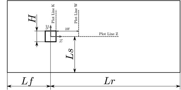
Figure 1: Sketch of the square section cylinder computational domain, side view, with plot lines

While some authors [29], [37] tested different methods to enforce a certain level of turbulence at the inflow to recreate the conditions at the inflow of the experiment [30], we decided for simplicity to use a uniform inflow condition, as done by other authors in different contexts, e.g. [49], [51], [57]. Wall adhesion conditions are imposed on the cylinder and Dirichlet conditions with far field values on the inflow and outflow sides, with sponge layers to dampen the disturbances and avoid reflections, as discussed for example in [10], [43]. On the upper and lower sides, Neumann boundary conditions are imposed, while in the spanwise direction periodic boundary conditions are enforced. The mesh used has 23816 tetrahedra and uses a structured block around the cylinder, to better control the element anisotropy, while being fully unstructured in the rest of the domain; this allows obtain an adequate resolution on the cylinder sides, without an excessive number of elements in the far field, as would happen with a fully extruded mesh. A two-dimensional side view of the mesh is presented in figure 2.

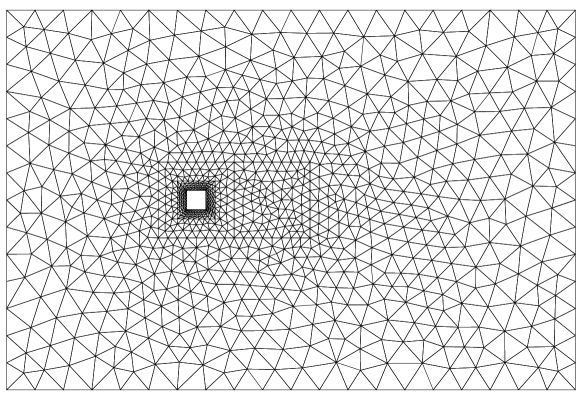
Figure 2: Two dimensional side view of the grid

Starting from a uniform initial condition, the simulation is evolved until statistical steady state is achieved. The resulting fields are used as a starting condition for the simulations described in the following, in which statistics are accumulated for around 16 shedding periods, averaging first along the spanwise direction and then in time. After this time span, which is indeed longer than the averaging time prescribed in [58], flow statistics showed only minor modifications. Statistics will be then presented as plots along three lines in the $x-y$ plane, as illustrated in figure 1.

4.1 Constant degree simulations

Some standard non adaptive simulations have been performed, to obtain a reference for the adaptive simulations with respect to the quality of results and the required computational effort. Three different simulations have been performed on the same grid with uniform polynomial degree equal to 2, 3 and 4. The grid has been dimensioned to be comparable with other similar computations [33], [49] using polynomial degree 4, thus the simulation at lower degree are considerably under-resolved. The subgrid model used for all the square cylinder computations is the Smagorinsky model described in section 2. While more refined subgrid models have been already tested in the present computational framework, see e.g. [1], our goal here was to carry out the analysis of adaptive approaches with the simplest possible subgrid model. The impact of more sophisticated models is the subject of ongoing work.

The global results, as well as computational data are presented in table 3. The Strouhal number is generally over-predicted with respect to the experimental values, as well as the drag coefficient and fluctuations. Some of these trends are reported also by other authors performing LES simulations, see e.g. [29], [33], [35], [37], while the general over prediction of force coefficients might be due to the low compressibility effects introduced here but not in any of the other references.

	St	<Cd>	rms(Cd’)	rms(Cl’)	dofs	core h.
experiments	$\approx 0.13$	$\approx 2.1$	$\approx 0.18$	$\approx 1.2$	-	-
degree 2	0.1462	2.321	0.148	1.204	238160	785
degree 3	0.1487	2.352	0.1605	1.305	476320	2665
degree 4	0.1410	2.398	0.1930	1.374	833560	7561

Table 3: Experimental and reference values of global quantities

The profiles of some velocity statistics and total turbulent stresses (resolved and modelled) are presented in figures 4.1, 4.1 and 5, measured along a line in the wake center, a line across the wake two diameters downstream and a vertical line over the rear corner of the cylinder. First of all, when increasing the polynomial degree, we observe a substantial convergence of the numerical solution to the experimental values in the wake, while over the rear corner of the cylinder the results are closer for all the different polynomial orders employed. The solutions computed with degree 2 are unsatisfactory in many areas, but more interestingly the solutions with degree 3, while being generally better than the degree 2 ones, are not a substantial improvement in the wake, where only the discretization with degree 4 gives acceptable results.

As noted above for the global results, these profiles are in general agreement with the experimental results, but still there are some discrepancies, which may be caused by employing compressible equations, or the lack of turbulence at inlet. The mismatch with experimental measurements is similar to the one observed in other computations, e.g. [37], [44], [49]. Notice that even experimental records such as those reported in [30] show a lack of agreement with other experimental data beyond 3 diameters downstream in the wake. The lower velocity far from the wake in figure 4(a) is instead clearly caused by the lower blockage of the cylinder in the simulation with respect to the experiment.

Since the simulations have been performed in different conditions than the experiments with which they have been are compared, some discrepancies, especially in the wake area, are justifiable and the results can be considered accurate enough. Therefore, for the following adaptive simulations, the main reference will be the refined constant degree simulations, rather than experimental results.

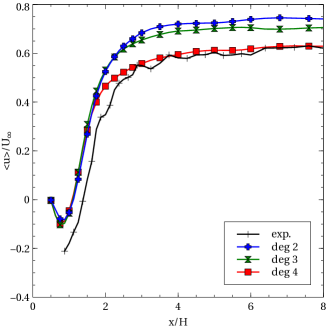
(a) streamwise mean velocity

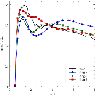
(b) square root of total turbulent stresses, xx component

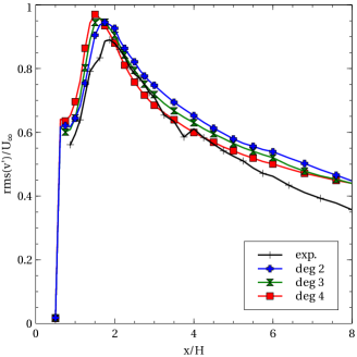
(c) square root of total turbulent stresses, yy component

Figure 3: Velocity statistics in the wake of the cylinder along plot line Z (see fig. 1), comparison of the results with different uniform polynomial degree

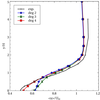
(a) Streamwise mean velocity

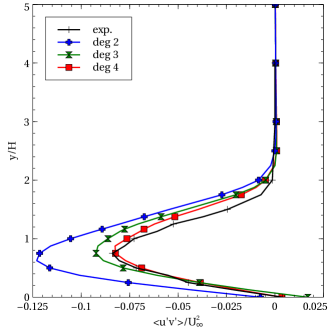
(b) total turbulent stresses, xy component

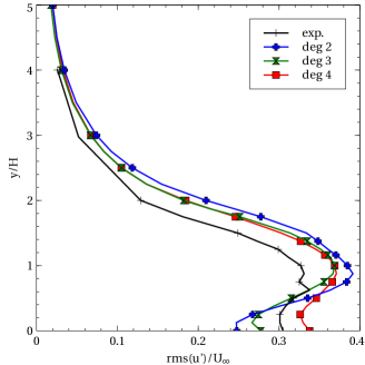
(c) square root of total turbulent stresses, xx component

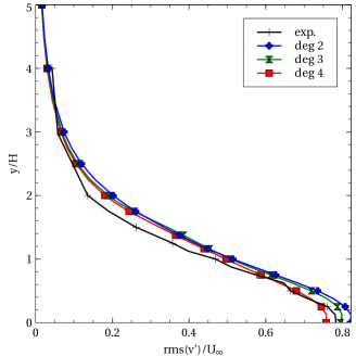
(d) square root of total turbulent stresses, yy component

Figure 4: Velocity statistics across the wake of the cylinder, along plot line W (see fig. 1), comparison of the results with different uniform polynomial degree

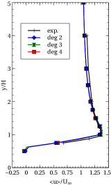
(a) Streamwise mean velocity

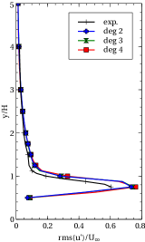
(b) square root of total turbulent stresses, xx component

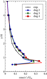
(c) square root of total turbulent stresses, yy component

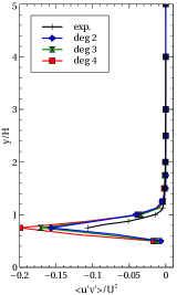
(d) total turbulent stresses, xy component

Figure 5: Velocity statistics over the cylinder in correspondence of the rear corner, along plot line K (see fig. 1), comparison of the results with different uniform polynomial degree

4.2 Validation of the adaptive simulations

After the reference solutions have been obtained, adaptive simulations have been performed. The aim of the adaptive computations presented in the following is to validate the adaptation procedure, to assess the quality of the results compared with the reference non adaptive results, to compare the performances of the proposed indicators and to check the reduction in computational effort with respect to the non adaptive simulation. The adaptation procedure was based on indicators computed on preliminary runs that employed constant polynomial degree equal to 4, thus thwarting the reduction in computational effort obtained with the adaptation. This however allows us to validate the proposed approach, while adaptive simulations based on cheaper adaptation procedure and yielding a net reduction of the computational effort will be presented in the following section 4.3.

Both the indicator based on modal coefficients (M) and the structure function (SF) indicator introduced in section 3 have been computed based on the results obtained from a preliminary simulation with constant degree 4. Two threshold values $\epsilon_{1}$ $\epsilon_{2}$ have been chosen for each indicator. The threshold values were selected to obtain a reasonable amount of degrees of freedom and an acceptable distribution of polynomial degrees, as well as to obtain a comparable number of degrees of freedom for the two adaptive simulations. More specifically, for the indicator based on modal coefficients (M) the values $\epsilon_{1}=0.075,$ $\epsilon_{2}=0.113$ were used, while for the structure function (SF) the values $\epsilon_{1}=5\times 10^{-4},$ $\epsilon_{2}=1\times 10^{-2}$ were used. The cells with indicator values smaller than $\epsilon_{1}$ have been assigned polynomial degree 2, those with indicator values larger than $\epsilon_{2}$ have been assigned polynomial degree 4, while the others have been assigned polynomial degree 3. The adaptive simulations have been initialized with appropriate local projections of the previous uniform degree 4 results.

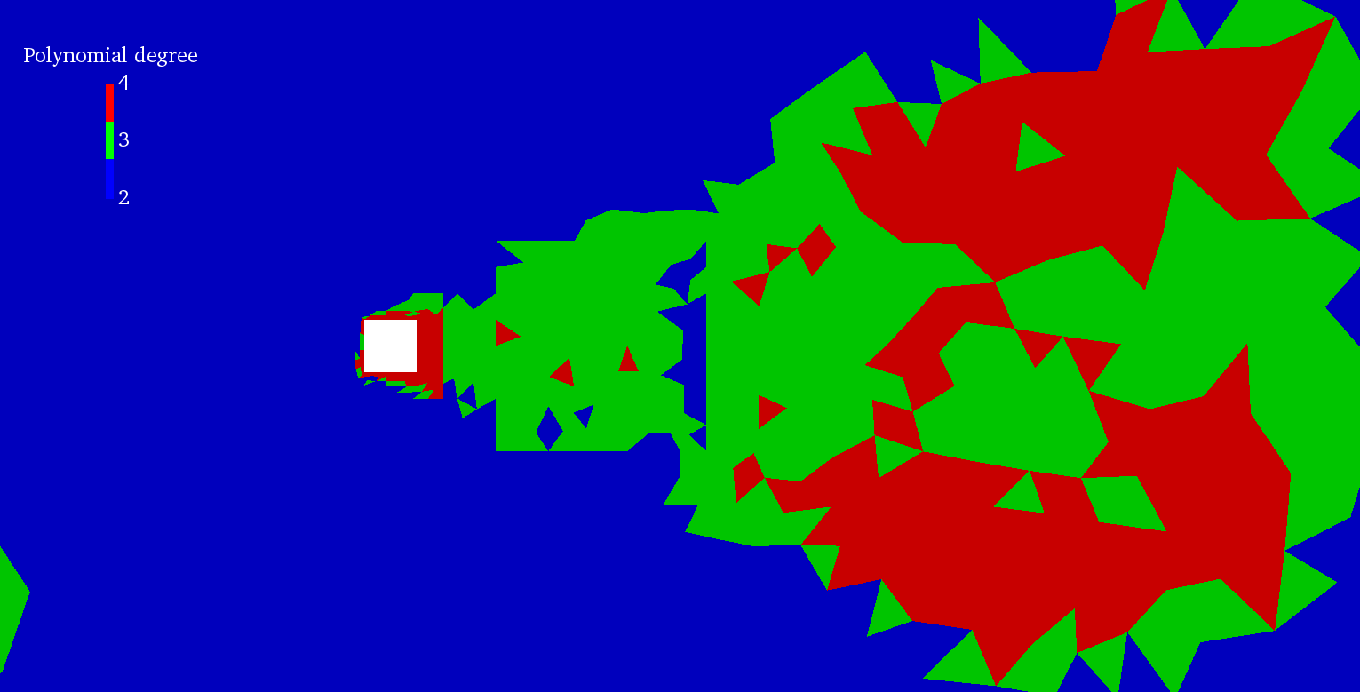
(a) M indicator

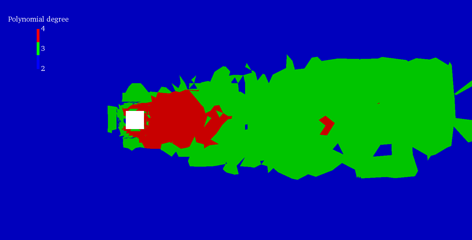
(b) SF indicator

Figure 6: Map of the polynomial degree of the elements, on a vertical slice, for the two different indicators

Both refinement indicators generally show larger values in the wake of the cylinder and lower values away from it, as it is predictable and desirable. The M indicator yields a narrower range of values, from $O(10^{-4})$ to $O(10^{-1})$, with larger values more scattered in the wake, meaning that the high order elements are distributed over a wider area. The SF indicator yields instead a broader value range, from $O(10^{-12})$ to $O(1)$, with the larger values concentrated in the near wake of the cylinder and in the shear layer generated by the separations after the front vertexes of the cylinder. In the wake, the indicator takes intermediate values, while outside the wake it reaches very low values. This allows to identify more clearly the area to be refined. The resulting polynomial distributions are shown in figure 4.2, on a 2D plane perpendicular to the spanwise direction. Along the spanwise direction, the degree distribution is almost uniform and small differences are due to the fact that the mesh is not uniform in that direction. The polynomial distribution in case of the M indicator shows a narrow high order zone in close proximity of the cylinder wall, and a broader higher order area far in the wake of the cylinder. In case of the SF indicator, the high order area is mainly confined in the near wake of the cylinder and around the forward corners, and generally the more refined zone has approximately at the same width throughout the wake.

The domain decomposition for adaptive parallel runs was performed using the METIS library [25], as in the non adaptive ones. However, in order to ensure an efficient load balancing, each cell has been assigned a different weight in the graph partitioning algorithm, based on the element polynomial degree. Some experiments have been performed by using different powers of the number of degrees of freedom of the element, as a weight, but in the end the simple weighting by the number of element degrees of freedom resulted in the the best parallel load balance.

	St	<Cd>	rms(Cd’)	rms(Cl’)	dofs	core h.
degree 4	0.1410	2.398	0.1930	1.374	833560	7561
adaptive M	0.1594	2.293	0.1319	1.191	398160	2949
adaptive SF	0.1410	2.350	0.1692	1.241	398270	2662

Table 4: Global quantities in $p-$adaptive simulations

The global data of the adaptive simulations are presented in table 4, compared with the uniform degree 4 simulation. It is clear that the values obtained from the simulation with the SF indicator are closer to those of the full degree 4 simulation than those obtained from the simulation performed with the M indicator. With respect to the full degree 4 simulation, there is a reduction of $52\%$ of the degrees of freedom from both simulations and a mean reduction of the computational time of around $60\%$. Notice that, when considering $p-$adaptation, the computational cost is not directly proportional to the number of degrees of freedom, since within a high order element more degrees of freedom are coupled with each other. Hence, reducing the number of high order elements has a beneficial effect that goes beyond the mere reduction of the total number of degrees of freedom. Fluctuations in the computational time are due to possible unbalances during parallel runs.

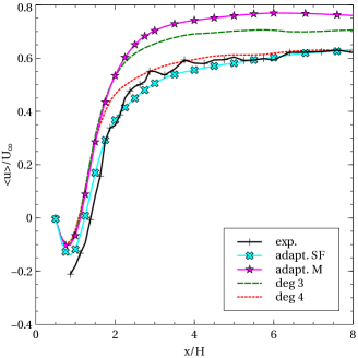
(a) streamwise mean velocity

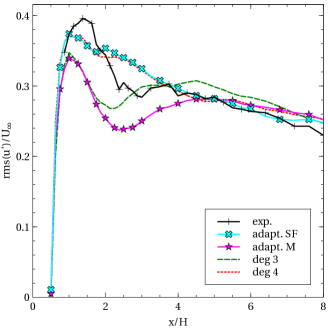
(b) square root of total turbulent stresses, xx component

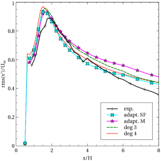
(c) square root of total turbulent stresses, yy component

Figure 7: Velocity statistics in the wake of the cylinder, along plot line Z (see fig. 1), adaptive solutions compared with uniform degree solutions and experimental data

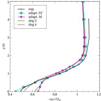
(a) Streamwise mean velocity

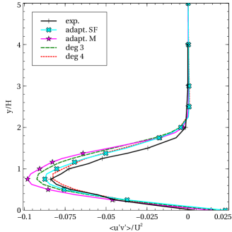
(b) total turbulent stresses, xy component

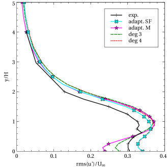
(c) square root of total turbulent stresses, xx component

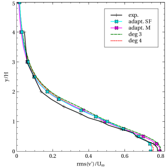
(d) square root of total turbulent stresses, yy component

Figure 8: Velocity statistics across the wake of the cylinder, along plot line W (see fig. 1), adaptive solutions compared with uniform degree solutions and experimental data

The profiles of the velocity statistics are presented in figures 4.2 and 4.2. It is evident that in most cases the results obtained with the SF indicator are much closer to the reference results, while using the M indicator leads, with the same number of degrees of freedom, to results closer to those obtained with uniform degree 3, which as discussed previously are not satisfactory. It is worth noting that, for both adaptive simulations, the number of degrees of freedom is slightly smaller than that in the full degree 3 simulation, while the computational time is comparable. Summarizing, adapting the solution according to the M indicator allows to have results similar to those of the uniform degree 3 simulations with similar effort, i.e. it does not affect negatively the results, but only yields a small improvement. On the other hand, using the SF indicator it is possible to obtain results comparable to those of a degree 4 solution with the effort of a degree 3 solution.

Given the presented results, the SF indicator appears to be more robust and to lead to more accurate results. In this context of static adaptivity, where the indicator calculation is performed as a local postprocessing task between a initial run and the actual adaptive run, the additional computational cost due to the more complex indicator is negligible. During the static indicator computation, only a few hundreds of full instantaneous fields from a previous run are processed and the impact of the indicator calculation is limited. In fact, all indicators calculations did not exceed a few minutes of CPU time on a personal computer. The cost of the indicator calculation will be surely larger in future dynamically adaptative runs, where the need to have a time resolved adaptation and a statistically reliable indicator evaluation will lead to more frequent evaluations of the indicator.

Considering the results with the perspective of adaptation based on the physical local conditions of the flow, as discussed in sections 1 and 3, it is possible to correlate the better results obtained with the SF indicator to the fact that it allows to have a better physical insight on the actual flow conditions than the M indicator. This encourages pursuing the study of other possible adaptation criteria based on the evaluation of the local flow properties.

4.3 Sensitivity of the adaptive simulation on the resolution of the indicator computation

Some simple sensitivity tests have been performed with respect to the data used to calculate the indicator and the resulting polynomial distributions. While keeping the rest of the procedure, thresholds included, identical to that described in section 4.2, we have used as data for the indicator calculation the results from

• a different degree 4 simulation with identical setup as the one presented in section 4.1

• the results obtained with the uniform degree 2 simulation presented in section 4.1.

In the first case the aim is to test the variability of the final results of the adaptivity procedure starting from different realizations of the same simulation. In the second, we wanted to investigate whether it was possible to use the much less expensive degree 2 results to calculate the indicator, thus obtaining a real reduction in computational time with respect to the uniform degree simulations. In both cases, the polynomial distribution obtained is close to the one obtained from degree 4, first realization, shown in figure 6(b).

The global data are presented in table 5, while velocity statistics profiles are shown in figures 4.3 and 4.3. Both in the global results and in the statistics profiles, the simulation performed with the indicator calculated from the two different realizations shows some variability in spite of the similar polynomial distribution. However, the differences between the results are clearly smaller with respect to those between simulations performed with lower constant polynomial degree and the reference simulation, or those between results achieved with different adaptation indicators and the reference simulation. Therefore, the adaptive simulation does not appear to be especially sensitive to the preliminary run data. Even more interestingly, it can be seen that the results obtained with the polynomial distribution calculated from low degree preliminary runs, fall within the same variability range as the results based on the degree 4 results.

	St	<Cd>	rms(Cd’)	rms(Cl)	dofs	core h.
P4	0.1410	2.398	0.1930	1.374	833560	7561
AP4R1	0.1410	2.350	0.1692	1.241	398270	2662
AP4R2	0.1425	2.400	0.1486	1.380	397210	2560
AP2	0.1483	2.390	0.1642	1.338	398105	2640

Table 5: Global quantities from different simulations with SF indicator for sensitivity analysis: P4) constant degree 4, AP4R1) adaptive simulation with SF criterion computed from degree 4 simulation, AP4R2) adaptive simulation with SF criterion computed from a different degree 4 simulation, AP2) adaptive simulation with SF criterion computed from degree 2 simulation.

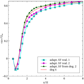
(a) streamwise mean velocity

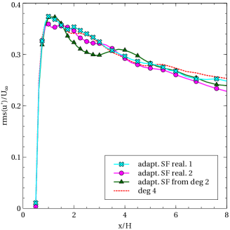
(b) square root of total turbulent stresses, xx component

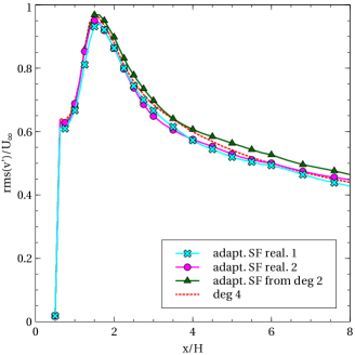
(c) square root of total turbulent stresses, yy component

Figure 9: Velocity statistics in the wake of the cylinder, along plot line Z (see fig. 1), comparison of results based on indicators calculated from different data

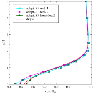
(a) Streamwise mean velocity

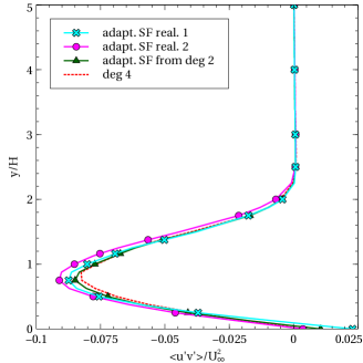
(b) total turbulent stresses, xy component

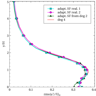
(c) square root of total turbulent stresses, xx component

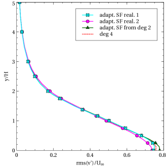
(d) square root of total turbulent stresses, yy component

Figure 10: Velocity statistics across the wake of the cylinder, along plot line Z (see fig. 1), comparison of results based on indicators calculated from different data

This simulations show not only that the adaptation procedure is robust, but also that it is possible to obtain good results based on an indicator computed from a very coarse preliminary simulation, which itself is inexpensive and produces unsatisfactory results as shown in figures 4.1 and 4.1. The coarse simulation contains however enough information to allow an effective adaptation and accurate results from the following adaptive simulation. The total core hours used to obtain the results from degree 2, starting from zero, is 3682, comprising the time needed to achieve a statistical stationary state, accumulate statistics at constant degree 2, a buffer time in the adapted configuration to allow the transition at the new degree distribution and the statistics accumulation time in the adapted configuration. This figure is around just $38\%$ of the 9778 core hours needed to obtain the full degree 4 polynomial base results starting from zero, and shows that the static adaptation procedure is not only effective in terms of quality of the results, but allows for a substantial computational effort reduction also when approaching a new case without refined reference results, which is the most realistic situation.

5 Conclusions and future perspectives

We have introduced and tested a novel approach for adapting the local polynomial degree in the DG discretization of a compressible LES model. The proposed indicator tries to measure the local turbulence intensity in the flow by computing an approximation of the structure function, rather than computing a local error estimate. The novel indicator performance has been compared to that of more conventional adaptation criteria using the flow around a bluff body as benchmark. Static adaptivity based on preliminary model runs has been performed. Both indicators were capable of highlighting domain areas of major turbulent activity, but the indicator based on the evaluation of the structure function proved itself more capable to lead to accurate results than the one based on the relative weight of the modal solution. Results obtained with the novel indicator led to accurate results, comparable to those obtained with constant maximum polynomial degree, with a reduction of the computational effort of approximately 60%. A sensitivity analysis has also been carried out, showing that an accurate adaptive solution can be achieved using a relatively coarse resolution in the preliminary runs, thus outlining a practical procedure to obtain efficient adaptive results with minimal additional effort.

The adaptation procedure in the LES context has been shown to be effective, in spite of the complexities and peculiarities illustrated in section 1. The use of physically based indicators produced satisfactory results and proved to be a good candidate to overcome the difficulties related to adaptive LES. Given this encouraging results, on one hand we plan to keep investigating also other indicators capable to easily assess the local flow conditions from the LES viewpoint. On the other hand, we are currently developing a dynamic adaptation procedure based on the same approach proposed in this paper. In this way we hope to extend the benefits of adaptation to statistically non stationary phenomena, such as vortex interaction, moving boundaries and general transient phenomena.

Appendix A Structure function form in homogeneous isotropic turbulence

We report here the calculations necessary to obtain an analytical expression of the isotropic form of the structure function from a calculated structure function, and then to evaluate the difference between the isotropic form and the calculated structure function. Given the structure function

$$D_{ij}(\boldsymbol{r},\boldsymbol{x},t)=\left\langle\left[U_{i}(\boldsymbol{x}+\boldsymbol{r},t)-U_{i}(\boldsymbol{x},t)\right]\left[U_{j}(\boldsymbol{x}+\boldsymbol{r},t)-U_{j}(\boldsymbol{x},t)\right]\right\rangle$$

and its corresponding expression in the isotropic case

$$D_{ij}^{iso}(\boldsymbol{r},t)=D_{NN}(r,t)\delta_{ij}+\left(D_{LL}(r,t)-D_{NN}(r,t)\right)\frac{r_{i}r_{j}}{r^{2}},$$ (20bj)

it is possible to define a quadratic error

$$Q=\left[D_{ij}^{iso}-D_{ij}\right]^{2}=\left[D_{ij}^{iso}-D_{ij}\right]\left[D_{ij}^{iso}-D_{ij}\right]$$ (20bk)

which, thanks to the definition 20bj becomes:

$$Q=\left[D_{NN}(r,t)\delta_{ij}+\left(D_{LL}(r,t)-D_{NN}(r,t)\right)\frac{r_{i}r_{j}}{r^{2}}-D_{ij}\right]^{2}.$$ (20bl)

Looking for the values of $D_{LL}$ and $D_{NN}$ which minimize the error, the following system of equations must be solved:

$$\frac{\partial Q}{\partial D_{NN}}=0,\ \ \ \frac{\partial Q}{\partial D_{LL}}=0,$$

which becomes

$$\left[D_{NN}(r,t)\delta_{ij}+\left(D_{LL}(r,t)-D_{NN}(r,t)\right)\frac{r_{i}r_{j}}{r^{2}}-D_{ij}\right]\left(\delta_{ij}-\frac{r_{i}r_{j}}{r^{2}}\right)=0$$

$$\left[D_{NN}(r,t)\delta_{ij}+\left(D_{LL}(r,t)-D_{NN}(r,t)\right)\frac{r_{i}r_{j}}{r^{2}}-D_{ij}\right]\left(\frac{r_{i}r_{j}}{r^{2}}\right)=0.$$

Noting that $\delta_{ij}\delta_{ij}=3,$ $\delta_{ij}A_{ij}=\operatorname{tr}\left(A_{ij}\right)$ and

$$\operatorname{tr}\left(\frac{r_{i}r_{j}}{r^{2}}\right)=\frac{r^{2}}{r^{2}}=1,$$

the final formulation becomes

$$D_{NN}=\frac{D_{ij}\frac{r_{i}r_{j}}{r^{2}}-\operatorname{tr}\left(D_{ij}\right)\left(\frac{r_{i}r_{j}}{r^{2}}\right)^{2}}{1-3\left(\frac{r_{i}r_{j}}{r^{2}}\right)^{2}}$$

$$D_{LL}=D_{NN}\left(\operatorname{tr}\left(D_{ij}\right)-2\right).$$

Finally, once the two coefficients $D_{NN},$ $D_{LL}$ have been computed, it is possible to evaluate the quantity $Q$ using equation 20bl.

References

- [1] A. Abbà, L. Bonaventura, M.Nini, and M. Restelli. Dynamic models for Large Eddy Simulation of compressible flows with a high order DG method. Computers & Fluids, 122:209–222, 2015.
- [2] I. Babuska, C.E. Baumann, and J.T. Oden. A discontinuous finite element method for diffusion problems: 1-D analysis. Computers Mathematics with Applications, 37(9):103–122, 1999.
- [3] P. W. Bearman and E. D. Obasaju. An experimental study of pressure fluctuations on fixed and oscillating square-section cylinders. Journal of Fluid Mechanics, 119:297–321, 1982.
- [4] A. D. Beck, T. Bolemann, D. Flad, H. Frank, G. J. Gassner, F. Hindenlang, and C.-D. Munz. High-order discontinuous galerkin spectral element methods for transitional and turbulent flow simulations. International Journal for Numerical Methods in Fluids, 76(8):522–548, 2014.
- [5] A. Burbeau and P. Sagaut. A dynamic adaptive discontinuous Galerkin method for viscous flow with shocks. Computers & Fluids, 34:401–2417, 2005.
- [6] B. Cockburn and C. Shu. The Local Discontinuous Galerkin Method for Time-Dependent Convection-Diffusion Systems. SIAM Journal of Numerical Analysis, 35:2440–2463, 1998.
- [7] S. S. Collis. Discontinuous Galerkin methods for turbulence simulation. In Proceedings of the 2002 Center for Turbulence Research Summer Program, pages 155–167, 2002.
- [8] S. S. Collis and Y. Chang. The DG/VMS method for unified turbulence simulation. AIAA paper, 3124:24–27, 2002.
- [9] R. Cools. An Encyclopaedia of Cubature Formulas. Journal of Complexity, 19:445–453, 2003.
- [10] A. Crivellini. Assessment of a sponge layer as a non-reflective boundary treatment with highly accurate gust–airfoil interaction results. International Journal of Computational Fluid Dynamics, 30(2):176–200, 2016.
- [11] L. Demkowicz, J.T. Oden, W. Rachowicz, and O.C. Hardy. An Taylor-Galerkin finite element method for compressible Euler equations. Computer Methods in Applied Mechanics and Engineering, 88:363–396, 1991.
- [12] L. Demkowicz, W. Rachowicz, and P. Devloo. An fully automatic adaptivity. Journal of Scientific Computing, 17:117–142, 2002.
- [13] T.M. Eidson. Numerical simulation of turbulent rayleigh-bénard problem using subgrid modeling. Journal of Fluid Mechanics, 158:245–268, 1985.
- [14] G. Erlebacher, M.Y. Hussaini, C.G. Speziale, and T.A. Zang. Large-eddy simulation of compressible turbulent flows. Journal of Fluid Mechanics, 238:155–185, 1992.
- [15] C. Eskilsson. An -adaptive discontinuous Galerkin method for shallow water flows. International Journal of Numerical Methods in Fluids, 67:1605–1623, 2011.
- [16] FEMilaro, a finite element toolbox. https://bitbucket.org/mrestelli/femilaro/wiki/Home. Available under GNU GPL v3.
- [17] D. Flad, A. Beck, and C.-D. Munz. Simulation of underresolved turbulent flows by adaptive filtering using the high order discontinuous galerkin spectral element method. Journal of Computational Physics, 313:1–12, 2016.
- [18] J.E. Flaherty and P.K. Moore. Integrated space-time adaptive -refinement methods for parabolic systems. Applied Numerical Mathematics, 16:317–341, 1995.
- [19] M. Germano. Turbulence: the filtering approach. Journal of Fluid Mechanics, 238:325–336, 1992.
- [20] F.X. Giraldo and M. Restelli. A study of spectral element and discontinuous Galerkin methods for the Navier-Stokes equations in nonhydrostatic mesoscale atmospheric modeling: equation sets and test cases. Journal of Computational Physics, 227:3849–3877, 2008.
- [21] J. Hoffman. Computation of Mean Drag for Bluff Body Problems Using Adaptive DNS/LES. SIAM Journal on Scientific Computing, 27(1):184–207, 2005.
- [22] J. Hoffman and C. Johnson. Stability of the dual Navier-Stokes equations and efficient computation of mean output in turbulent flow using adaptive DNS/LES. Computer Methods in Applied Mechanics and Engineering, 195(13-16):1709–1721, 2006.
- [23] P. Houston and E. Süli. A note on the design of hp-adaptive finite element methods for elliptic partial differential equations. Computational methods in applied mechanics and engineering, 194:229–243, 2005.
- [24] J. Jimenez. A selection of test cases for the validation of large-eddy simulations of turbulent flows. Advisory Report AGARD-AR-345, AGARD, 1998.
- [25] G. Karypis and V. Kumar. A fast and high quality multilevel scheme for partitioning irregular graphs. SIAM Journal on scientific Computing, 20(1):359–392, 1998.
- [26] D. Knight, G. Zhou, N. Okong’o, and V.Shukla. Compressible large eddy simulation using unstructured grids. Technical Report 98-0535, American Institute of Aeronautics and Astronautics, 1998.
- [27] B. Koobus and C. Farhat. A variational multiscale method for the large eddy simulation of compressible turbulent flows on unstructured meshes—-application to vortex shedding. Computer Methods in Applied Mechanics and Engineering, 193:1367–1383, 2004.
- [28] B. Landmann, M. Kessler, S. Wagner, and E. Krämer. A parallel, high-order discontinuous galerkin code for laminar and turbulent flows. Computers & Fluids, 37:427–438, 2008.
- [29] Z. Liu. Investigation of Flow Characteristics Around Square. Engineering Applications of Computational Fluid Mechanics, 6(3):426–446, 2012.
- [30] D. A. Lyn, S. Einav, W. Rodi, and J.-H. Park. A laser-doppler velocimetry study of ensemble-averaged characteristics of the turbulent near wake of a square cylinder. Journal of Fluid Mechanics, 304:285–319, 12 1995.
- [31] D. a. Lyn and W. Rodi. The flapping shear layer formed by flow separation from the forward corner of a square cylinder. Journal of Fluid Mechanics, 267:353, 1994.
- [32] I. McLean and I. Gartshore. Spanwise correlations of pressure on a rigid square section cylinder. Journal of Wind Engineering and Industrial Aerodynamics, 41(1-3):797–808, 1992.
- [33] M. Minguez, C. Brun, R. Pasquetti, and E. Serre. Experimental and high-order LES analysis of the flow in near-wall region of a square cylinder. International Journal of Heat and Fluid Flow, 32(3):558–566, 2011.
- [34] M. Minguez, R. Pasquetti, and E. Serre. Spectral LES of turbulent flows over bluff bodies: from the square cylinder to a car model. In BBAA VI International Colloquium on: Bluff Bodies Aerodynamics & Applications, 2008.
- [35] M. Minguez, R. Pasquetti, and E. Serre. Spectral LES of turbulent flows over bluff bodies: from the square cylinder to a car model. In BBAA VI International Colloquium on: Bluff Bodies Aerodynamics & Applications, 2008.
- [36] Sorin M. Mitran. A Comparison of Adaptive Mesh Refinement Approaches for Large Eddy simulations. In Chaoqun Liu, editor, Third AFOSR International Conference on Direct Numerical Simulation and Large Eddy Simulation (TAICDL), pages 397–408, 2001.
- [37] S. Murakami, S. Iizuka, and R. Ooka. Cfd Analysis of Turbulent Flow Past Square Cylinder Using Dynamic Les. Journal of Fluids and Structures, 13(7-8):1097–1112, 1999.
- [38] S. Murakami and A. Mochida. On turbulent vortex shedding flow past 2D square cylinder predicted by CFD. Journal of Wind Engineering and Industrial Aerodynamics, 54-55:191–211, 1995.
- [39] C. Norberg. Flow around rectangular cylinders: Pressure forces and wake frequencies. Journal of Wind Engineering and Industrial Aerodynamics, 49(1-3):187–196, 1993.
- [40] S. B. Pope. Turbulent Flows, volume 1. 2000.
- [41] S. B. Pope. Ten questions concerning the large-eddy simulation of turbulent flows. New journal of Physics, 6(1):35, 2004.
- [42] J.F. Remacle, J.E. Flaherty, and M.S. Shephard. An adaptive Discontinuous Galerkin technique with an orthogonal basis applied to compressible flow problems. SIAM Review, 45:53–72, 2003.
- [43] M. Restelli and F.X. Giraldo. A conservative Discontinuous Galerkin semi-implicit formulation for the Navier-Stokes equations in nonhydrostatic mesoscale modeling. SIAM Journal of Scientific Computing, 31:2231–2257, 2009.
- [44] W. Rodi. Comparison of LES and RANS calculations of the flow around bluff bodies. Journal of Wind Engineering and Industrial Aerodynamics, 69-71:55–75, 1997.
- [45] W Rodi, J H Ferziger, M Breuer, and M Pourquie. Status of Large Eddy Simulation: Results of a workshop. Journal of Fluids Engineering, Transactions of the ASME, 119(2):248–262, 1997.
- [46] P. Sagaut. Large Eddy Simulation for Incompressible Flows: An Introduction. Springer Verlag, 2006.
- [47] K. Sengupta, F. Mashayek, and G.B. Jacobs. Large eddy simulation using a discontinuos galerkin spectral method. In 45th AIAA Aerospace Sciences Meeting and Exhibit. AIAA, AIAA-2007-402 2007.
- [48] J. Smagorinsky. General circulation experiments with the primitive equations: part I, the basic experiment. Monthly Weather Review, 91:99–162, 1963.
- [49] A. Sohankar and L. Davidson. Large Eddy Simulation of flow past a square cylinder: Comparison of different subgrid scale models. Journal of Fluids Engineering, Transactions of the ASME, 122(March 2000):39–47, 2000.
- [50] R.J. Spiteri and S.J. Ruuth. A New Class of Optimal High-Order Strong-Stability-Preserving Time Discretization Methods. SIAM Journal of Numerical Analysis, 40:469–491, 2002.
- [51] F. X. Trias, A. Gorobets, and A. Oliva. Turbulent flow around a square cylinder at Reynolds number 22,000: A DNS study. Computers and Fluids, 123(22):87–98, 2015.
- [52] G. Tumolo and L. Bonaventura. A semi-implicit, semi-Lagrangian, DG framework for adaptive numerical weather prediction. Quarterly Journal of the Royal Meteorological Society, 141:2582–2601, 2015.
- [53] G. Tumolo, L. Bonaventura, and M. Restelli. A semi-implicit, semi-Lagrangian, p-adaptive Discontinuous Galerkin method for the shallow water equations. Journal of Computational Physics, 232:46–67, 2013.
- [54] A. Uranga, P.O. Persson, M. Drela, and J. Peraire. Implicit Large Eddy Simulation of transition to turbulence at low Reynolds numbers using a Discontinuous Galerkin method. International Journal for Numerical Methods in Engineering, 87:232–261, 2011.
- [55] F. van der Bos and B.J. Geurts. Computational error-analysis of a Discontinuous Galerkin discretization applied to large-eddy simulation of homogeneous turbulence. Computer Methods in Applied Mechanics and Engineering, 199:903–915, 2010.
- [56] F. van der Bos, J.J.W. van der Vegt, and B.J. Geurts. A multi-scale formulation for compressible turbulent flows suitable for general variational discretization techniques. Computer Methods in Applied Mechanics and Engineering, 196:2863–2875, 2007.
- [57] R W C P Verstappen and a E P Veldman. Spectro-consistent discretization of Navier-Stokes : a challenge to RANS and LES. Journal of Enginnering Mathematics, 34:163–179, 1998.
- [58] P. R. Voke. Flow Past a Square Cylinder: Test Case LES2, pages 355–373. Springer Netherlands, 1997.
- [59] L. Wei and A. Pollard. Direct numerical simulation of compressible turbulent channel flows using the Discontinuous Galerkin method. Computers and Fluids, 47:85–100, 2011.
- [60] L. Zhang, T. Cui, and H. Liu. A set of symmetric quadrature rules on triangles and tetrahedra. J. Comput. Math, 27(1):89–96, 2009.
- [61] O.C. Zienkiewicz, J.P. Gago, and D.W. Kelly. The hierarchical concept in finite element analysis. Computers and Structures, 16:53–65, 1983.
- [62] O.C. Zienkiewicz and J.Z. Zhu. Adaptivity and mesh generation. International Journal for Numerical Methods in Engineering, 32:783–810, 1991.