The Bramson logarithmic delay in the cane toads equations

Abstract

We study a nonlocal reaction-diffusion-mutation equation modeling the spreading of a cane toads population structured by a phenotypical trait responsible for the spatial diffusion rate. When the trait space is bounded, the cane toads equation admits traveling wave solutions [7]. Here, we prove a Bramson type spreading result: the lag between the position of solutions with localized initial data and that of the traveling waves grows as $(3/(2\lambda^{*}))\log t$. This result relies on a present-time Harnack inequality which allows to compare solutions of the cane toads equation to those of a Fisher-KPP type equation that is local in the trait variable.

1 Introduction

The cane toads spreading

Cane toads were introduced in Queensland, Australia in 1935, to control the native cane beetles in sugar-cane fields. Initially, about one hundred cane toads were released, and by now, their population is estimated to be about two hundred million, leading to disastrous ecological effects. Their invasion has interesting features different from the standard spreading observed in most other species [31]. Rather than invade at a constant speed, the annual rate of progress of the toad invasion front has increased by a factor of about five since the toads were first introduced: the toads expanded their range by about 10 km a year during the 1940s to the 1960s, but were invading new areas at a rate of over 50 km a year by 2006. Toads with longer legs move faster and are the first to arrive to new areas, followed later by those with shorter legs. In addition, those at the front have longer legs than toads in the long-established populations – the typical leg length of the advancing population at the front grows in time. The leg length is greatest in the new arrivals and then declines over a sixty year period. The cane toads are just one example of a non-uniform space-trait distribution – one other is the expansion of the bush crickets in Britain [34]. There, the difference is between the long-winged and short-winged crickets, with similar conclusions. In all such phenomena, modelling of the spreading rates has to include the trait structure of the population.

The cane toads equation

We consider here a model of the cane toads invasion proposed in  [3], based on the classical Fisher-KPP equation [18, 23]. The population density $n(t,x,\theta)$ is structured by a spatial variable $x$, and a motility variable $\theta$. This population undergoes diffusion in the trait variable $\theta$, with a constant diffusion coefficient, representing mutation, and in the spatial variable, with the diffusion coefficient $\theta$, representing the effect of the trait on the spreading rates of the species. In addition, each toad competes locally in space with all other individuals for resources. If the competition is local in the trait variable, then the corresponding Fisher-KPP model is

$$u_{t}=\theta u_{xx}+u_{\theta\theta}+u(1-u).$$ (1.1)

It is much more biologically relevant to consider a non-local in trait competition (but still local in space), which leads to

$$n_{t}=\theta n_{xx}+n_{\theta\theta}+rn(1-\rho),$$ (1.2)

where

$$\rho(t,x)=\int_{\Theta}n(t,x,\theta)d\theta$$ (1.3)

is the total population at the position $x$. Here, $\Theta$ is the set of all possible traits. It is either an infinite semi-interval: $\Theta=[\underline{\theta},+\infty)$, or an interval $\Theta=[\underline{\theta},\overline{\theta}]$. For simplicity, we consider the one-dimensional case: $x\in{\mathbb{R}}$. Both (1.1) and (1.2) are supplemented by Neumann boundary conditions at $\theta=\underline{\theta}$ and $\theta=\overline{\theta}$ (in the case when $\Theta$ is a finite interval):

$$n_{\theta}(t,x,\underline{\theta})=n_{\theta}(t,x,\overline{\theta})=0,~{}~{}t>0,~{}x\in{\mathbb{R}}.$$ (1.4)

The cane toads equation is but one example among other non-local reaction models that have been extensively studied recently [1, 4, 10, 17, 22, 26, 27]. Mathematically, non-local models are particularly interesting since their solutions do not obey the maximum principle and standard propagation results for the scalar local reaction-diffusion equations do not apply. Rather, on the qualitative level they behave as solutions of systems of reaction-diffusion equations, for which much fewer spreading results are available. The study of the spreading of solutions to the cane toads equations started with a Hamilton-Jacobi framework that was formally developed in [8], and rigorously justified in [35] when $\Theta$ is a finite interval. Existence of the travelling waves for (1.2) in that case has been proved in [7].

As far as unbounded traits are concerned, a formal argument in [8] using a Hamilton-Jacobi framework predicted front acceleration, observed in the field, and the spreading rate of $O(t^{3/2})$. A rigorous proof of this spreading rate has been given in [6, 9].

The main results

In this paper, we consider the spreading rate of the solutions of the non–local cane toads equation (1.2)-(1.3), with $x\in{\mathbb{R}}$ and $\theta\in\Theta=[\underline{\theta},\overline{\theta}]$, and the Neumann boundary conditions (1.4). The initial condition $n(0,x,\theta)=n_{0}(x,\theta)\not\equiv 0$ is non-negative and has localized support in a sense to be made precise later. The classical result of [18, 23] says that solutions of the scalar KPP equation

$$v_{t}=v_{xx}+v(1-v)$$ (1.5)

with a non-negative compactly supported initial condition $v_{0}(x)=v(0,x)$ propagate with the speed $c^{*}=2$ in the sense that

$$\lim_{t\to+\infty}v(t,ct)=0,$$ (1.6)

for all $c>c^{*}$, and

$$\lim_{t\to+\infty}v(t,ct)=1,$$ (1.7)

for all $c\in[0,c^{*}]$. The corresponding result for the solutions of (1.2) follows from the Hamilton-Jacobi limit in [35]. The Fisher-KPP result for the solutions of (1.5) has been refined by Bramson in [11, 12]. He has shown the following: for any $m\in(0,1)$, let

$$X_{m}(t)=\sup\{x:~{}v(t,x)=m\},$$

with $s\in(0,1)$. This level set has the asymptotics

$$X_{m}(t)=2t-\frac{3}{2}\log t+x_{m}+o(1),~{}~{}\hbox{ as $t\to+\infty$}.$$ (1.8)

Here, $x_{m}$ is a constant that depends on $m$ and the initial condition $v_{0}$. Bramson’s original proof was probabilistic. A shorter probabilistic proof can be found in a recent paper [32], while the PDE proofs can be found in [24, 36] and, more recently, in [20]. Various extensions to equations with inhomogeneous coefficients have also been studied in [14, 15, 21, 25, 28]. In this paper, we establish a version of (1.8) – but with the weaker $O(1)$ correction rather than $o(1)$ as in (1.8) – for the solutions of the non-local cane toads equation (1.2). We will assume that the initial condition is compactly supported on the right: there exists $x_{0}$ such that $n_{0}(x)=0$ for all $x\geq x_{0}$. It has been shown in [7] that (1.2)-(1.4) admits a travelling wave solution of the form $n(t,x,\theta)=\phi(x-c^{*}t,\theta)$. It is expected that the function $\phi(\xi,\theta)$ has the asymptotic decay

$$\phi(\xi,\theta)\sim\xi e^{-\lambda^{*}\xi}Q(\theta),$$ (1.9)

with a uniformly positive function $Q(\theta)>0$. While [7] does not show that travelling waves exist for all $c>c^{*}$, this is expected. This would imply that $c^{*}$ is the minimal speed of propagation for the cane toads equation, in the same sense as $\tilde{c}^{*}=2$ is the minimal speed of propagation for the Fisher-KPP equation (see also [7, Remark 4]). A precise characterization of the minimal speed $c^{*}$ and the decay rate $\lambda^{*}$ from [7] is recalled in Section 4.1. Here is our main result.

Theorem 1.1.

Let $n(t,x,\theta)$ satisfy the system (1.2)-(1.4), with the initial condition $n_{0}(x)\geq 0$ satisfying the assumptions above. There exists $m_{0}$ such that for all $\varepsilon\in(0,m_{0})$, there is a positive constant $C_{\varepsilon}$ such that

$$\begin{split}&\liminf_{t\to\infty}\inf_{x\leq c^{*}t-\frac{3}{2\lambda^{*}}\log(t)-C_{\varepsilon}}n(t,x)\geq m_{0}-\varepsilon,\\ &\limsup_{t\to\infty}\sup_{x\geq c^{*}t-\frac{3}{2\lambda^{*}}\log(t)+C_{\varepsilon}}n(t,x)\leq\varepsilon.\end{split}$$

The main difficulty in the proof of Theorem 1.1 is the lack of the maximum principle. In order to circumvent this, we obtain a present-time Harnack inequality for $n$, described below, which is of an independent interest. Using this, we reduce the problem to showing the logarithmic delay for the local Fisher-KPP system (1.1), a much simpler problem, as it obeys the maximum principle. The analysis for the local equation follows the general strategy of [21], with some non-trivial modifications.

A parabolic Harnack inequality

We will make use of the following version of the Harnack inequality, that is new, to the best of our knowledge. Consider an operator

$$Lu=\sum_{ij}a_{ij}(x)\frac{\partial^{2}u}{\partial x_{i}\partial x_{j}}.$$ (1.10)

Here, $A(x):=\left(a_{ij}(x)\right)$ is a Hölder continuous, uniformly elliptic matrix: there exist $\lambda>0$ and $\Lambda>0$ such that

$$\forall x\in\mathbb{R}^{n},\qquad\lambda I\leq A(x)\leq\Lambda I,$$

in the sense of matrices.

Theorem 1.2.

Suppose that $u$ is a positive solution of

$$u_{t}-Lu=0,~{}t>0,~{}x\in{\mathbb{R}}^{n}.$$ (1.11)

For any $t_{0}>0$, $R>0$, and $p>1$, there exists a constant $C$ such that if $t\geq t_{0}$ and $|x-y|\leq R$, then

$$u(t,x)\leq C\|u_{0}\|_{\infty}^{1-1/p}u(t,y)^{1/p}.$$ (1.12)

Moreover, $C$ depends only on $\lambda$, $\Lambda$, $n$, $t_{0}$, $R$, and $p$.

We point out that Theorem 1.2 does not hold with $p=1$. Indeed, when $n=1$ and $(a_{ij})=I$, the solution $u(t,x)=t^{-1/2}\exp\left\{-x^{2}/4t\right\}$ does not satisfy (1.12).

The paper is organized as follows. First, we prove Theorem 1.2 in Section 2. Then, in Section 3, we use the Harnack inequality to reduce the spreading rate question for the non-local cane toads equation to that for the local problem (1.1). Section 4 contains the proof of the corresponding result for the local equation, with its most technical part presented in Section 5.

Acknowledgement. EB was supported by “INRIA Programme Explorateur”. LR was supported by NSF grant DMS-1311903. Part of this work was performed within the framework of the LABEX MILYON (ANR- 10-LABX-0070) of Université de Lyon, within the program ÒInvestissements dÕAvenirÓ (ANR-11- IDEX-0007) operated by the French National Research Agency (ANR). In addition, CH has received funding from the European Research Council (ERC) under the European Unions Horizon 2020 research and innovation programme (grant agreement No 639638).

2 A present-time parabolic Harnack inequality

In this section, we prove Theorem 1.2. It is a consequence of a small time heat kernel estimate due to Varadhan [37]. Let $G(t,x,y)$ be the fundamental solution to (1.11):

$$\begin{cases}G_{t}=L_{x}G,~{}~{}t>0,~{}~{}x,y\in{\mathbb{R}}^{n},\\ G(0,\cdot,y)=\delta(\cdot-y),\end{cases}$$ (2.1)

so that the solution of

$$\begin{cases}u_{t}-Lu=0,~{}~{}~{}t>0,~{}~{}x\in{\mathbb{R}}^{n},\\ u(0,x)=u_{0}(x),\end{cases}$$

can be written, for all $t>0$ and $x\in\mathbb{R}^{n}$, as

$$u(t,x)=\int_{\mathbb{R}^{n}}G(t,x,y)u_{0}(y)dy.$$

The notation $L_{x}$ in (2.1) means that the operator $L$ acts on $G$ in the $x$ variable. There are well-known Gaussian bounds for $G$ (see e.g. [2, 13]) of the type

$$\frac{c_{1}}{t^{n/2}}e^{-c_{2}\frac{|x-y|^{2}}{t}}\leq G(t,x,y)\leq\frac{C_{1}}{t^{n/2}}e^{-C_{2}\frac{|x-y|^{2}}{t}},$$

for $(t,x,y)\in\mathbb{R}^{+}\times\mathbb{R}^{n}\times\mathbb{R}^{n}$. However, these are not precise enough in their dependence on $x$ and $y$ for our purposes, as they do not control the constants $c_{2}$ and $C_{2}$ very well.

To state Varadhan’s estimate, we introduce some notation. Given a matrix $A(x)=(a_{ij}(x))$, the associated Riemannian metric $d_{A}$ is

$$d_{A}(x,y)=\inf_{\begin{subarray}{c}p\in C^{1}([0,1]),\\ p(0)=x,p(1)=y\end{subarray}}\int_{0}^{1}\sqrt{\dot{p}(\tau)A^{-1}(p(\tau))\dot{p}(\tau)}d\tau.$$

The ellipticity condition on the matrix $A$ implies that $d_{A}$ and $|\cdot|$ yield equivalent metrics.

Theorem 2.1 (Theorem 2.2 [37]).

The limit

$$\lim_{t\to 0}\left(-4t\log G(t,x,y)\right)=d_{A}(x,y)^{2}$$

holds uniformly for all $x$ and $y$ such that $|x-y|$ is bounded.

This agrees with the usual heat kernel when $L=\Delta$ since then $A=I$ and $d_{A}(x,y)=|x-y|$. We may not use this result as stated as we will require a uniform estimate over all $x$ and $y$, without a restriction to a compact set. However, it is easy to check that the proof in [37], with a few straightforward modifications, implies the following.

Theorem 2.2.

Given any $\varepsilon>0$, the following inequalities hold uniformly over all $x,y\in{\mathbb{R}}^{n}$:

$$\liminf_{t\to 0}\big{[}-4t\log G(t,x,y)\big{]}\geq(1-\varepsilon)d_{A}(x,y)^{2},$$ (2.2)

$$\limsup_{t\to 0}\big{[}-4t\log G(t,x,y)\big{]}\leq(1+\varepsilon)d_{A}(x,y)^{2}.$$

We can now proceed with the proof of Theorem 1.2.

Proof of Theorem 1.2.

Without loss of generality we may assume that $y=0$ and $|x|\leq R$ in (1.12). Let us take $t_{0}>0$ and write, for all $t>t_{0}$ and $x\in\mathbb{R}^{n}$:

$$u(t,x)=\int_{\mathbb{R}^{n}}G(t_{0},x,y)u(t-t_{0},y)dy.$$

We have, using the maximum principle, with some $s\in(0,1)$, to be specified later:

$$\begin{split}u(t,x)&=\int_{\mathbb{R}^{n}}G(t_{0},x,z)u(t-t_{0},z)dz\\ &\leq\|u(t-t_{0},\cdot)\|_{\infty}^{1/q}\int_{\mathbb{R}^{n}}\left(u(t-t_{0},z)G(t_{0},x,z)^{sp}\right)^{1/p}\left(G(t_{0},x,z)^{(1-s)q}\right)^{1/q}dz\\ &\leq\|u_{0}\|_{\infty}^{1/q}\left(\int_{\mathbb{R}^{n}}u(t-t_{0},z)G(t_{0},x,z)^{sp}dz\right)^{1/p}\left(\int_{\mathbb{R}^{n}}G(t_{0},x,z)^{(1-s)q}dz\right)^{1/q}\\ &\leq C\|u_{0}\|_{\infty}^{1/q}\left(\int_{\mathbb{R}^{n}}u(t-t_{0},z)G(t_{0},x,z)^{sp}dz\right)^{1/p}.\end{split}$$ (2.3)

Here, we have chosen $q\in(1,\infty)$ satisfies

$$\frac{1}{p}+\frac{1}{q}=1,$$

and the constant $C>0$ depends on $t_{0}$ (in particular, it blows up as $t_{0}\downarrow 0$). The last inequality in (2.3) is an application of the bounds in (2.2) since $s<1$. Our next step is to show and use the following inequality: there exist a constant $C>0$ and $s>1/p$ that both depend on $t_{0}$, $R$, and $p$ such that

$$G(t_{0},x,y)^{sp}\leq CG(t_{0},0,y),$$ (2.4)

for all $y\in{\mathbb{R}}^{n}$ and $|x|\leq R$.

Before proving (2.4), we shall conclude the proof of Theorem 1.2. Using (2.4) in (2.3) gives

$$u(t,x)\leq C\|u_{0}\|_{\infty}^{1/q}\left(\int_{\mathbb{R}^{n}}u(t-t_{0},y)G(t_{0},0,y)dy\right)^{1/p}=C\|u_{0}\|_{\infty}^{1/q}u(t,0)^{1/p},$$ (2.5)

which is (1.12) with $y=0$.

To establish (2.4), we choose $s\in(0,1)$, $\varepsilon>0$ and $\theta\in(0,1)$ such that

$$sp(1-\varepsilon)>1+\varepsilon,$$ (2.6)

and

$$1-\theta=\frac{(1+\varepsilon)}{sp(1-\varepsilon)}.$$

We may now use Theorem 2.2 to choose $t_{0}$ small enough so that

$$\begin{split}&-4t_{0}\log G(t_{0},x,y)\geq(1-\varepsilon)d_{A}(x,y)^{2}-\varepsilon,\\ &-4t_{0}\log G(t_{0},x,y)\leq(1+\varepsilon)d_{A}(x,y)^{2}+\varepsilon,\end{split}$$ (2.7)

for all $x,y\in{\mathbb{R}}^{n}$. Using (2.7) and the triangle inequality

$$d_{A}(x,y)\geq|d_{A}(x,0)-d_{A}(0,y)|,$$

we get

$$\begin{split}\log[G(t_{0},x,y)^{sp}]-\frac{sp\varepsilon}{4t_{0}}&\leq-sp(1-\varepsilon)\frac{d_{A}(x,y)^{2}}{4t_{0}}\\ &\leq-sp(1-\varepsilon)\frac{d_{A}(x,0)^{2}-2d_{A}(x,0)d_{A}(y,0)+d_{A}(y,0)^{2}}{4t_{0}}.\end{split}$$

Young’s inequality yields that

$$\log[G(t_{0},x,y)^{sp}]-\frac{sp\varepsilon}{4t_{0}}\leq\left(\frac{1}{\theta}-1\right)\frac{sp(1-\varepsilon)d_{A}(x,0)^{2}}{4t_{0}}-\frac{sp(1-\varepsilon)(1-\theta)d_{A}(y,0)^{2}}{4t_{0}}.$$

Using the definition of $\theta$ and that the Euclidean metric and $d_{A}$ are equivalent, we deduce

$$\log[G(t_{0},x,y)^{sp}]-\frac{sp\varepsilon}{4t_{0}}\leq\frac{CR^{2}}{t_{0}}-\frac{(1+\varepsilon)d_{A}(y,0)^{2}}{4t_{0}},$$

with a constant $C>0$ that depends on $\theta$, $p$ and $\varepsilon$. Applying the bounds in (2.7) again, we obtain

$$\log[G(t_{0},x,y)^{sp}]-\frac{sp\varepsilon}{4t_{0}}\leq\frac{CR^{2}}{t_{0}}+\log G(t_{0},0,y)+\frac{\varepsilon}{4t_{0}}.$$

Exponentiating, we get (2.4), finishing the proof.

∎

3 A reduction to the local cane toads problem

In this section, we show how to compare solutions of the non-local cane toads equation to the solutions of a local cane toads problem, of a more general form than (1.1). To do this, we use Theorem 1.2 to eliminate the non-local term in (1.2). This will allow us to find two local cane toads equations to which the solution of (1.2) is a sub- and super-solution, respectively.

It has been shown in [35], that solutions of (1.2) satisfy a uniform bound

$$n(t,x,\theta)\leq M$$ (3.1)

for all $(t,x,\theta)\in[0,\infty)\times\mathbb{R}\times\Theta$ with a constant $M$ depending only on $\underline{\theta}$ and $\overline{\theta}$. With this in hand, we first show that we may bootstrap Theorem 1.2 to hold for $n$ as well.

Proposition 3.1.

For any $t_{0}>0$, $R>0$, and $p>1$, there is a constant $C>0$ such that if $t\geq t_{0}$ and $|\theta-\theta^{\prime}|+|x-x^{\prime}|\leq R$, and $n$ is a solution of (1.2)-(1.4), then

$$n(t,x,\theta)\leq Cn(t,x^{\prime},\theta^{\prime})^{1/p}.$$ (3.2)

Proof of Proposition 3.1.

The proof is by comparing $n$ to a solution to an associated linear heat equation. Take $t_{1}\geq t_{0}$ and let $h$ be the solution to

$$h_{t}=\theta h_{xx}+h_{\theta\theta},$$

with the Neumann boundary conditions

$$h_{\theta}(t,x,\underline{\theta})=h_{\theta}(t,x,\overline{\theta})=0,$$

and the initial condition

$$h(0,x,\theta)=n(t_{1}-\delta,x,\theta),$$

with $\delta=\min\{1,t_{0}/2\}$. Theorem 1.2 implies that there is a constant $C$ depending only on $M$, $\delta$, $R$ and $p$ such that, for any $|x-x^{\prime}|\leq R$ and $\theta\in[\underline{\theta},\overline{\theta}]$, we have

$$h(t,x,\theta)\leq Ch(t,x^{\prime},\theta)^{1/p},$$

for all $t\geq\delta$.

On the other hand, as

$$n(1-M|\Theta|)\leq n(1-\rho)\leq n,$$

the comparison principle implies that

$$e^{(1-M|\Theta|)t}h(t,x)\leq n(t_{1}-\delta+t,x)\leq e^{t}h(t,x).$$

Hence, we may pull the Harnack inequality from $h$ to $n$: for all $(x,\theta)\in\mathbb{R}\times\Theta$ and $(x^{\prime},\theta^{\prime})\in\mathbb{R}\times\Theta$ such that $|x-x^{\prime}|+|\theta-\theta^{\prime}|\leq R$ we have

$$n(t_{1},x,\theta)\leq e^{\delta}h(\delta,x,\theta)\leq Ce^{\delta}h(\delta,x^{\prime},\theta^{\prime})^{1/p}\leq Ce^{\delta}\left(e^{(M|\Theta|-1)\delta}n(t_{1},x^{\prime},\theta^{\prime})\right)^{1/p}.$$

This finishes the proof.

∎

We now construct two local cane toads problems for which $n$ is a sub- and super-solution. We fix $p\in(1,3/2)$ and find $C>0$ so that we may apply Proposition 3.1 with $t_{0}=1$ and $R=|\Theta|$, to obtain (after integration)

$$\frac{n(t,x,\theta)^{p}}{C^{p}}\leq\rho(t,x)\leq Cn(t,x,\theta)^{1/p}.$$

for all $t\geq 1$, $x\in\mathbb{R}$ and $\theta\in\Theta$. It follows that

$$n\left(1-Cn^{1/p}\right)\leq n(1-\rho)\leq n\left(1-\frac{n^{p}}{C^{p}}\right).$$ (3.3)

This implies that for $t\geq 1$ the function $n(t,x,\theta)$ is a super-solution to the equation

$$\underline{u}_{t}-\theta\underline{u}_{xx}-\underline{u}_{\theta\theta}=\underline{u}(1-C\underline{u}^{1/p}),$$ (3.4)

and a sub-solution to the equation

$$\overline{u}_{t}-\theta\overline{u}_{xx}-\overline{u}_{\theta\theta}=\overline{u}\left(1-C^{-p}\overline{u}^{p}\right).$$ (3.5)

Here, $\underline{u}$ and $\overline{u}$ satisfy the same Neumann boundary conditions (1.4) as $n$.

We now choose the initial conditions at $t=0$: $\underline{u}_{0}(x,\theta)=\underline{u}(0,x,\theta)$ and $\overline{u}_{0}(x,\theta)=\overline{u}(0,x,\theta)$, so that the ordering

$$\underline{u}(t=1,x,\theta)\leq n(t=1,x,\theta)\leq\overline{u}(t=1,x,\theta)$$ (3.6)

holds for all $x$ and $\theta$. This will guarantee that

$$\underline{u}(t,x,\theta)\leq n(t,x,\theta)\leq\overline{u}(t,x,\theta)$$ (3.7)

for all $t\geq 1$ and all $x$ and $\theta$, because of (3.3). We only describe how $\underline{u}_{0}$ is chosen, but the process is similar for $\overline{u}_{0}$.

To this end, let $h$ be a solution to the equation

$$h_{t}-\theta h_{xx}-h_{\theta\theta}=0,$$ (3.8)

with the initial condition $h_{0}(x,\theta)=n_{0}(x,\theta)$. Define the function $\underline{h}=e^{(1-M|\Theta|)t}h$, which satisfies

$$\underline{h}_{t}=\theta\underline{h}_{xx}+\underline{h}_{\theta\theta}+\left(1-M|\Theta|\right)\underline{h},$$

where $M$ is the upper bound for $n$ from (3.1). Notice that $n$ is a super-solution to $\underline{h}$. Hence

$$n(t=1,x,\theta)\geq\underline{h}(t=1,x,\theta)=e^{\left(1-M|\Theta|\right)}h(t=1,x,\theta),$$ (3.9)

for all $x$ and $\theta$. On the other hand, for any $a>0$, the function

$$\overline{h}=ae^{t}h$$ (3.10)

is a super-solution for the equation for $\underline{u}$ (3.4). Hence, if $\underline{u}$ is the solution of (3.4) with the initial condition $\underline{u}_{0}=an_{0}$, then

$$\underline{u}(t=1,x,\theta)\leq aeh(t=1,x,\theta).$$ (3.11)

Putting (3.9) and (3.11) together gives us

$$\underline{u}(t=1,x,\theta)\leq ae^{M|\Theta|}n(1,x,\theta)$$

for all $x$ and $\theta$. Thus, if we choose $a=\exp(-M|\Theta|)$ then the first inequality in (3.6) holds. Similarly, we may choose an initial condition $\bar{u}_{0}$ so that the second inequality in (3.6) holds as well.

4 The logarithmic correction in the local cane toads fronts

We have shown that there exist functions $\underline{u}$ and $\overline{u}$, satisfying the local cane toads equations (3.4) and (3.5), respectively, such that the solution $n$ of (1.2)-(1.4) satisfies the lower and upper bounds in (3.7). Therefore, Theorem 1.1 is a consequence of the corresponding result for the Fisher-KPP equations. We present the local Fisher-KPP result in a slightly greater generality than what is needed for Theorem 1.1, as the extra generality introduces no extra complications in the proof.

Let $D$ be a uniformly positive and bounded function on a smooth domain $\Theta\subset\mathbb{R}^{d}$, and let $A$ be a $C^{1}$ function on $\Theta$. Let $u$ be the solution to the Fisher-KPP equation

$$u_{t}-Du_{xx}-\Delta_{\theta}u+Au_{x}=f(u),$$ (4.1)

with the Neumann boundary conditions:

$$\dfrac{\partial{u}}{\partial{\nu_{\theta}}}(t,x,\theta)=0,$$ (4.2)

and the initial condition $u(0,\cdot)=u_{0}$. Here, $\nu_{\theta}$ is the normal to $\partial\Theta$. We assume that

$$\liminf_{x\to-\infty}u_{0}(x,\theta)>0,$$ (4.3)

uniformly in $\theta\in\Theta$, that $u_{0}\geq 0$, and that there is some $x_{0}$ such that $u_{0}(x,\theta)=0$ for all $x\geq x_{0}$. The nonlinearity $f$ is of the Fisher-KPP type: there exist $u_{m}>0$, $M>0$ and $\delta>2/3$ such that

$$f(0)=f(u_{m})=0 f(u)>0 u\in[0,u_{m}]$$,      for all , (4.4)

and

$$u-M_{\delta}u^{1+\delta}\leq f(u)\leq u,~{}~{}\text{ for all }u\in[0,u_{m}].$$ (4.5)

A classical result of Berestycki and Nirenberg [5] shows that (4.1) admits travelling wave solutions of the form $u(t,x,\theta)=\Phi(x-ct,\theta)$, with $\Phi(x,\theta)$ such that

$$-c\Phi_{x}-D\Phi_{xx}-\Delta_{\theta}\Phi+A\Phi_{x}=f(\Phi),~{}~{}$$ (4.6)

and $\Phi(-\infty,\cdot)=u_{m}$, and $\Phi(+\infty,\cdot)=0$. In addition, $\Phi$ satisfies the Neumann boundary conditions (4.2), and $0<\Phi(x,\theta)<u_{m}$ for all $x$ and $\theta$. Such travelling waves exist for all $c\geq c^{*}$, with the same $c^{*}$ as in Theorem 1.1, and the travelling wave corresponding to the minimal speed has the asymptotics

$$\Phi(\xi,\theta)\sim\alpha\xi e^{-\lambda^{*}\xi}Q(\theta),~{}~{}\hbox{ as $x\to+\infty$},$$

with the same exponential decay rate $\lambda^{*}$ and profile $Q$ as in (1.9). Once again, a precise description of $c^{*}$ and $\lambda^{*}$ in terms of an eigenvalue problem will be given in Section 4.1. What is important for us is that, as far as the function $f$ is concerned, both $c^{*}$ and $\lambda^{*}$ depend only on $f^{\prime}(0)$ but not, say, on $u_{m}$ or $\delta$.

By translating and scaling and by changing to a constant speed moving reference frame, if necessary, we may assume without loss of generality that $u_{m}=1$, $f^{\prime}(0)=1$, that the drift $A$ has mean-zero, and, finally, that the initial condition $u_{0}$ is not identically equal to zero on the half-cylinder $\{x>0,~{}\theta\in\Theta\}$.

Theorem 4.1.

Suppose that $D$ and $A$ are as above and $f$ satisfies (4.4)-(4.5). There exist $c^{*}>0$ and $\lambda^{*}>0$ that, as far as $f$ is concerned, depend only on $f^{\prime}(0)$, with the following property. Let $u$ satisfy (4.1)-(4.2), with the initial condition $u_{0}$ as above (4.3). Then, for any $m\in(0,u_{m})$, there exist $x_{m}>0$ and $T_{m}>0$, depending on $m$, such that if $t\geq T_{m}$ we have

$$\{x\in\mathbb{R}\,:\,\exists\theta\in\Theta,\,u(t,x,\theta)=m\}\subset\left[c^{*}t-\frac{3}{2\lambda^{*}}\log(t)-x_{m},c^{*}t-\frac{3}{2\lambda^{*}}\log(t)+x_{m}\right].$$ (4.7)

Theorem 1.1 follows from Theorem 4.1 and the bounds on $n$ in (3.7), in terms of the solutions of the Fisher-KPP equations (3.4) and (3.5). The reason is that $c^{*}$ and $\lambda^{*}$ for the two non-linearities in (3.4) and (3.5) coincide, hence the level sets of the corresponding solutions $\underline{u}$ and $\overline{u}$ of these two equations stay within $O(1)$ from each other, and (3.7) means that so do the level sets of the solution of (1.2).

The proof of Theorem 4.1 mostly follows the strategy of [21] where a similar result has been proved in the one-dimensional periodic case. A general multi-dimensional form of the Bramson shift is a delicate problem [33]. However, the particular form of the present problem allows us to streamline many of the details and modifies some of the steps in the proof. Typically, the spreading speed $c_{*}$ of the solutions of the Fisher-KPP type equations can be inferred from the linearized problem, that in the present case takes the form

$$u_{t}+Au_{x}=Du_{xx}+\Delta_{\theta}u+f^{\prime}(0)u.$$ (4.8)

The main qualitative difference between the solutions of (4.8) and those of the nonlinear Fisher-KPP problem is that the former grow exponentially in time on any given compact set, while the latter remain bounded. A remedy for that discrepancy is to consider (4.8) in a domain with a moving boundary: $x>X(t)$, with

$$X(t)=c^{*}t-r(t),$$ (4.9)

with the Dirichlet boundary condition $u(t,X(t),\theta)=0$. Then the shift $r(t)$ is chosen so that the solutions of the moving boundary problem remain $O(1)$ as $t\to+\infty$. It turns out that such “correct” shift is exactly

$$r(t)=\frac{3}{2\lambda^{*}}\log t,$$ (4.10)

as in (4.7). This allows to use them as sub- and super-solutions to the nonlinear Fisher-KPP equation, to prove that the front of the solutions to (4.1) is also located at a distance $O(1)$ from $X(t)$ given by (4.9)-(4.10), which is the claim of Theorem 4.1.

4.1 The eigenvalue problem defining $c^{*}$ and $\lambda^{*}$.

Let us first recall from [5] how $c^{*}$ and $\lambda^{*}$ are defined in Theorems 1.1 and 4.1. We look for exponential solutions of the linearized cane toads equation (4.8), with $f^{\prime}(0)=1$, of the form

$$u(t,x,\theta)=e^{-\lambda(x-ct)}Q_{\lambda}(\theta).$$ (4.11)

This leads to the following spectral problem on the cross-section $\Theta$ for the unique positive eigenfunction $Q_{\lambda}>0$:

$$\left\{\begin{array}[]{ll}\Delta_{\theta}Q_{\lambda}+(\lambda^{2}D+\lambda A-\lambda c(\lambda)+1)Q_{\lambda}(\theta)=0,&\qquad\hbox{ in $\Theta$},\vskip 6.0pt plus 2.0pt minus 2.0pt\\ \dfrac{\partial{Q_{\lambda}}}{\partial{\nu_{\theta}}}=0,&\qquad\hbox{ on $\partial\Theta$.}\end{array}\right.$$

We will use the normalization

$$\int_{\Theta}Q_{\lambda}(\theta)d\theta=1.$$ (4.12)

In other words, given $\lambda>0$, we solve the eigenvalue problem

$$\left\{\begin{array}[]{ll}\Delta_{\theta}Q_{\lambda}+(\lambda^{2}D+\lambda A)Q_{\lambda}(\theta)=\mu(\lambda)Q_{\lambda},&\qquad\hbox{ in $\Theta$,}\vskip 6.0pt plus 2.0pt minus 2.0pt\\ \dfrac{\partial{Q_{\lambda}}}{\partial{\nu_{\theta}}}=0,&\qquad\hbox{ on $\partial\Theta$.}\end{array}\right.$$ (4.13)

It has a unique positive eigenfunction $Q_{\lambda}$ corresponding to its principal eigenvalue $\mu(\lambda)$ – this is a standard consequence of the Krein-Rutman theorem. The positivity of $\mu(\lambda)$ easily follows by dividing (4.13) by $Q_{\lambda}$, integrating, and using the positivity of $Q_{\lambda}$ and the boundary conditions, along with the normalization

$$\int_{\Theta}A(\theta)d\theta=0.$$

Then, the speed $c(\lambda)$ is determined by

$$\mu(\lambda)=\lambda c(\lambda)-1,$$ (4.14)

that is,

$$c(\lambda)=\frac{1+\mu(\lambda)}{\lambda}.$$ (4.15)

We will use the notation, well-defined by the following proposition,

$$c^{*}=\min_{\lambda>0}c(\lambda),~{}~{}\lambda^{*}=\underset{\lambda>0}{\text{argmin}}\,c(\lambda),$$ (4.16)

and denote by $Q^{*}$ the corresponding eigenfunction.

Proposition 4.2.

The function $\lambda\mapsto c(\lambda)$ has a minimum $c^{*}$, and

$$c^{*}{\int_{\Theta}\left(Q^{*}\right)^{2}d\theta}={\int_{\Theta}[2\lambda^{*}D(\theta)+A(\theta)]\left(Q^{*}\right)^{2}d\theta}.$$ (4.17)

Further, we have $c^{\prime\prime}(\lambda^{*})>0$.

Proof of Proposition 4.2. Since $Q_{\lambda}\in{C}^{2}(\Theta)$ and satisfies Neumann boundary conditions, there exists $\theta_{0}$ such that $\Delta Q_{\lambda}(\theta_{0})=0$. We deduce from (4.1):

$$c(\lambda)=\frac{1}{\lambda}+A(\theta_{0})+\lambda D(\theta_{0}).$$

As the functions $A(\theta)$ and $D(\theta)$ are bounded, and $D(\theta)$ is uniformly positive, $c(\lambda)$ satisfies

$$c(\lambda)\underset{\lambda\to 0}{\sim}\frac{1}{\lambda},\qquad\lambda c(\lambda)=\mathcal{O}_{\lambda\to+\infty}(\lambda^{2}).$$

The continuity of the function $c(\lambda)$ implies the existence of a positive minimal speed $c^{*}$ and a smallest positive minimizer $\lambda^{*}$.

Differentiating (4.1) with respect to $\lambda$, we obtain

$$\left(-\lambda c^{\prime}(\lambda)-c(\lambda)+A+2\lambda D\right)Q_{\lambda}+\left(\lambda^{2}D+\lambda A-\lambda c(\lambda)+1\right)\frac{\partial Q_{\lambda}}{\partial\lambda}+\Delta_{\theta}\left(\frac{\partial Q_{\lambda}}{\partial\lambda}\right)=0.$$

Let us multiply by $Q_{\lambda}$ and integrate. We obtain, for all $\lambda>0$,

$$\int_{\Theta}\left(-\lambda c^{\prime}(\lambda)-c(\lambda)+A(\theta)+2\lambda D(\theta)\right)Q_{\lambda}^{2}d\theta=0.$$ (4.18)

In particular, for $\lambda=\lambda^{*}$, we have $c^{\prime}(\lambda^{*})=0$, and (4.17) follows. Finally, for the last claim, it is easy to see by differentiating twice (4.14) and using $c^{\prime}(\lambda^{*})=0$ that

$$c^{\prime\prime}(\lambda^{*})=\frac{\mu^{\prime\prime}(\lambda^{*})}{\lambda^{*}}.$$

In addition, the variational principle for the principal eigenvalue $\mu(\lambda)$ of (4.13) implies that $\mu(\lambda)$ is a convex function. A straightforward computation shows that actually $\mu^{\prime\prime}(\lambda^{*})>0$, thus $c^{\prime\prime}(\lambda^{*})>0$.

4.2 A “heat equation” bound for the local cane toads equation

Motivated by the exponential solutions, we may decompose a general solution $u(t,x,\theta)$ of the linearized Fisher-KPP equation (4.8) as

$$u(t,x,\theta)=e^{-\lambda^{*}(x-c^{*}t)}Q^{*}(\theta)p(t,x,\theta).$$ (4.19)

The function $p(t,x,\theta)$ then satisfies

$$p_{t}=Dp_{xx}+\Delta_{\theta}p-\left(2\lambda^{*}D+A\right)p_{x}+\frac{2}{Q^{*}}\nabla_{\theta}Q^{*}_{\theta}\cdot\nabla_{\theta}p,$$ (4.20)

with the Neumann boundary conditions

$$\dfrac{\partial{p}}{\partial{\nu_{\theta}}}=0,\qquad\hbox{ on $\partial\Theta$.}$$ (4.21)

If $D\equiv 1$ and $A\equiv 0$, then $Q^{*}\equiv 1$ and $c^{*}=2\lambda^{*}$, meaning that (4.20) is simply the standard heat equation in the frame moving with speed $c^{*}$. As we have mentioned, in order to keep the solutions of the linearized problem bounded, we need to impose the Dirichlet boundary condition at a moving boundary. The next proposition shows that, in general, the special form of the drift terms in (4.20) balances exactly so that the solutions decay as those of the heat equation, with the Dirichlet boundary condition imposed. We formulate it for a slightly more general equation than (4.20), which we will need below.

Proposition 4.3.

Let $\omega:\mathbb{R}^{+}\mapsto\mathbb{R}^{+}$, $\overline{\omega}$, $C$, and $T$ be such that

$$\tau\omega(\tau)\to\overline{\omega}\hbox{ as }\tau\to+\infty,\qquad\qquad|\omega^{\prime}(\tau)\tau^{2}|,(\tau+T)\,\omega(\tau)\leq C$$ (4.22)

and let $p_{0}$ be a non-zero, non-negative function such that that $p_{0}(x)=0$ for all $x>x_{0}$ and such that $\mathds{1}_{[0,\infty)}p_{0}$ is non-zero. Suppose that $p$ satisfies

$$(1-\omega)p_{\tau}=Dp_{xx}+\Delta_{\theta}p-\left(2\lambda^{*}D+A\right)p_{x}+\frac{2}{Q^{*}}\nabla_{\theta}Q^{*}\cdot\nabla_{\theta}p,~{}~{}$$ (4.23)

for $\tau>0$, $x>c^{*}\tau$, and $\theta\in\Theta$, with the Neumann boundary condition (4.21), the Dirichlet boundary condition for $\tau>0$,

$$p(\tau,c^{*}\tau,\cdot)=0,$$ (4.24)

and the initial condition $p(0,\cdot)=p_{0}$. There exists $T_{0}$ such that if $T\geq T_{0}$, then there exist $\sigma>0$ and $C>0$ that do not depend on $p_{0}$, and $\tau_{0}>0$ that may depend on $p_{0}$ such that

$$\frac{x-c^{*}\tau}{C\tau^{3/2}}\leq p(\tau,x,\theta)\leq\frac{C(x-c^{*}\tau)}{\tau^{3/2}},$$ (4.25)

for all $x\in[c^{*}\tau,c^{*}\tau+\sigma\sqrt{\tau}]$, all $\theta\in\Theta$ and all $\tau\geq\tau_{0}$.

As the proof is rather technical, we postpone it for the moment. Its proof is in Section 5.

4.3 The upper bound

We will now show how to deduce the statement of Theorem 4.1 from Proposition 4.3, starting with the upper bound. We will thus prove that the delay is at least $\frac{3}{2\lambda^{*}}\log(t)$ in the following sense:

$$\max\{x\in\mathbb{R}\,:\,\exists\theta\in\Theta,\,u(t,x,\theta)=m\}\leq c^{*}t-\frac{3}{2\lambda^{*}}\log(t)+x_{m},$$

for some constant $x_{m}$. The idea is to use the linearized problem with a moving Dirichlet boundary condition to create a suitable super-solution. Obviously, the Dirichlet boundary condition prevents the solution of this problem from being directly a super-solution. To overcome this, we show that the solution to the linearized equation is greater than $1$ near the moving boundary. Hence, after a suitable cut-off, it will be a true super-solution.

To this end, we consider the solution to the linearized problem with the Dirichlet boundary condition at $x=c^{*}t-r\log(1+t/T)$, with $r$ and $T$ to be determined:

$$\left\{\begin{array}[]{ll}z_{t}-Dz_{xx}-\Delta_{\theta}z+Az_{x}=z,&\hbox{ for }x>c^{*}t-r\log(1+t/T),\vskip 6.0pt plus 2.0pt minus 2.0pt\\ z(t,c^{*}t-r\log(1+t/T),\cdot)=0,&\vskip 6.0pt plus 2.0pt minus 2.0pt\\ \dfrac{\partial{z}}{\partial{\nu_{\theta}}}=0,&\hbox{ on }\partial\Theta,\vskip 6.0pt plus 2.0pt minus 2.0pt\\ z(0,\cdot)=u_{0}.\end{array}\right.$$ (4.26)

We make a time change

$$\tau=t-\frac{r}{c^{*}}\log\left(1+\frac{t}{T}\right).$$ (4.27)

By fixing $T$ large enough, depending only on $r$ and $c^{*}$, we may ensure that the function $h(\tau)=t$ is one-to-one, and

$$\frac{1}{h^{\prime}(\tau)}=1-\frac{r}{c^{*}(t+T)}=1-\frac{r}{c^{*}(\tau+T)+r\log(1+t/T)}=1-\frac{r}{c^{*}(\tau+T)}+O(\tau^{-3/2}).$$ (4.28)

To simplify the notation, we define

$$\omega(\tau)=1-\frac{1}{h^{\prime}(\tau)},~{}~{}|\omega^{\prime}(\tau)|=O(\tau^{-2}).$$ (4.29)

Notice that $\omega$ satisfies (4.22). The function $\tilde{z}(\tau,\cdot)=z(t,\cdot)$ satisfies

$$(1-\omega)\tilde{z}_{\tau}=\tilde{D}\tilde{z}_{xx}+\Delta_{\theta}\tilde{z}-A\tilde{z}_{x}+\tilde{z}.$$

Let $\tau\mapsto\alpha(\tau)$ be a function to be determined later, and decompose $\tilde{z}$ as

$$\tilde{z}(\tau,x,\theta)=\alpha(\tau)e^{-\lambda^{*}(x-c^{*}\tau)}Q^{*}(\theta)\tilde{p}(\tau,x,\theta).$$

The function $\tilde{p}$ satisfies

$$(1-\omega)\tilde{p}_{\tau}=D\tilde{p}_{xx}+\Delta_{\theta}\tilde{p}-(A+2\lambda D)p_{x}+\frac{2}{Q^{*}}\nabla_{\theta}Q^{*}\cdot\nabla_{\theta}\tilde{p}+\left(-\frac{\alpha^{\prime}}{h^{\prime}\alpha}+\frac{r\lambda^{*}}{t+T}\right)\tilde{p},$$ (4.30)

and $\tilde{p}(\tau,c^{*}\tau,\cdot)=0$ for all $\tau$. We choose $\alpha$ as the solution of

$$\frac{\alpha^{\prime}}{\alpha}=\frac{r\lambda^{*}}{t+T}h^{\prime}=\frac{r\lambda^{*}}{\tau+T}+O\left(\frac{1}{(\tau+T)^{2}}\right),$$ (4.31)

with the asymptotics:

$$\alpha(\tau)=\exp\left\{r\lambda^{*}\log(\tau+T)+O(\tau^{-1})\right\}=(\tau+T)^{r\lambda^{*}}(1+O(\tau^{-1})).$$ (4.32)

In view of (4.29), we may apply Proposition 4.3 to the solutions of (4.30). This, along with (4.32), implies that if we choose

$$r=\frac{3}{2\lambda^{*}},$$ (4.33)

then there exist constants $\sigma$, $C_{1}$ and $C_{2}$ and a fixed time $\tau_{0}$ such that we have

$$C_{1}(x-c^{*}\tau)e^{-\lambda^{*}(x-c^{*}\tau)}\leq\tilde{z}(\tau,x,\theta)\leq C_{2}(x-c^{*}\tau)e^{-\lambda^{*}(x-c^{*}\tau)},$$ (4.34)

for $\tau\geq\tau_{0}$ and all $x\in[c^{*}\tau,c^{*}\tau+\sigma\sqrt{\tau}]$. Hence, we may choose $M$ such that

$$M\tilde{z}(\tau,c^{*}\tau+1,\theta)\geq 2,$$

for all $\tau\geq\tau_{0}$ and $\theta\in\Theta$.

We may now define a super-solution for the nonlinear Fisher-KPP equation (4.1) as

$$\overline{u}(t,x,\theta)=\begin{cases}\min(1,Mz(t,x,\theta)),~{}~{}~{}~{}~{}~{}&\text{ for all }x\geq c^{*}t-r\log(1+t/T)+1,\vskip 6.0pt plus 2.0pt minus 2.0pt\\ 1,&\text{ for all }x\leq c^{*}t-r\log(1+t/T)+1.\end{cases}$$

Figure 1 depicts a sketch of the solution $u$ of the nonlinear Fisher-KPP problem, and the super-solution $\overline{u}$. We also have $\overline{u}(h(\tau_{0}),\cdot)\geq u_{0}$ for a sufficiently large $M$, since $u_{0}$ is compactly supported on the right. Hence, we have

$$u(t,\cdot)\leq\overline{u}(h(\tau_{0})+t,\cdot)$$

for all $t\geq t_{0}$.

To conclude, it follows from the form of our super-solution and (4.34) that, given any $m\in(0,1)$, we may choose $x_{m}\geq 1$ such that $\overline{u}(t,x,\theta)<m$ for all $t\geq t_{0}$, all

$$x\geq c^{*}t-\frac{3}{2\lambda^{*}}\log t+x_{m},$$

and all $\theta\in\Theta$. Thus, for such $x$ we have

$$u(t,x,\theta)\leq\bar{u}(t,x,\theta)\leq m,$$

for all $t\geq t_{0}$ and $\theta\in\Theta$. This concludes the proof of the upper bound in Theorem 4.1.

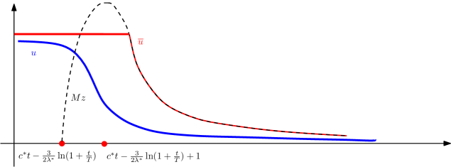
Figure 1: A sketch of the solution $u$ and the super-solution $\overline{u}$.

4.4 The lower bound

We now prove that the delay is at most $\frac{3}{2\lambda^{*}}\log(t)$ in the following sense:

$$\min\{x\in\mathbb{R}\,:\,\exists\theta\in\Theta,\,u(t,x,\theta)=m\}\geq c^{*}t-\frac{3}{2\lambda^{*}}\log(t)+x_{m},$$

for some constant $C_{m}$. The proof of the lower bound requires the same estimates as the upper bound, but the approach is slightly different. Note that the solution to the linearized equation is not a sub-solution to the nonlinear Fisher-KPP equation since $f(u)\leq u$. To get around this, we solve the linearized equation with a moving Dirichlet boundary condition at $c^{*}t$, instead of $c^{*}t-(3/2\lambda^{*})\log(t)$, in order to make this solution small. Then, we modify the solution to the linearized equation by an order $O(1)$ multiplicative factor in order to obtain a sub-solution.

The resulting sub-solution will decay in time. Hence, we may not directly conclude a lower bound on the location of the level sets. Instead, we show that this sub-solution is of the correct order $e^{-\sigma\sqrt{t}}/t$ at the position $c^{*}t+\sigma\sqrt{t}$. This will allow us to fit a travelling wave underneath the solution $u$ of the Fisher-KPP equation on the half-line $x<c^{*}t+\sigma\sqrt{t}$, and we use this travelling wave to obtain a lower bound on the location of the level sets of $u$. We will assume without loss of generality that

$$\ell:=\liminf_{x\to-\infty}\inf_{\theta\in\Theta}u_{0}(x,\theta)=1.$$ (4.35)

It is straightforward to modify the argument below to account for the case $\ell<1$. Note that $\ell>0$ by assumption (4.3). As a consequence of (4.44) we have that, for all $t\geq 0$,

$$\liminf_{x\to-\infty}\inf_{\theta\in\Theta}u(t,x,\theta)=1.$$ (4.36)

A preliminary sub-solution using the linearized system

As outlined above, the first step is to obtain a sub-solution decaying in time. To this end, we look at the solution $w$ to

$$\left\{\begin{array}[]{ll}w_{t}-Dw_{xx}-\Delta_{\theta}w+Aw_{x}=w,&\hbox{ for }x>c^{*}t,\vskip 6.0pt plus 2.0pt minus 2.0pt\\ w(t,c^{*}t,\cdot)=0,&\vskip 6.0pt plus 2.0pt minus 2.0pt\\ \dfrac{\partial{w}}{\partial{\nu_{\theta}}}=0,&\hbox{ on }\partial\Theta,\vskip 6.0pt plus 2.0pt minus 2.0pt\\ w(0,\cdot)=u_{0}.\end{array}\right.$$ (4.37)

As before, we factor out a decaying exponential, and the eigenfunction $Q^{*}$:

$$w(t,x,\theta)=e^{-\lambda^{*}(x-c^{*}t)}Q^{*}(\theta)p(t,x,\theta).$$ (4.38)

The function $p$ satisfies

$$p_{t}=Dp_{xx}+\Delta_{\theta}p-\left(2\lambda^{*}D+A\right)p_{x}+\frac{2}{Q^{*}}\nabla_{\theta}Q^{*}\cdot\nabla_{\theta}p_{\theta},~{}~{}~{}\text{ for $x>c^{*}t$, }$$ (4.39)

with the corresponding boundary and initial conditions. Proposition 4.3 with $\omega=0$ gives an upper bound

$$|p(t,x+c^{*}t)|\leq\frac{Cx}{(t+1)^{3/2}},$$

that, along with the decomposition (4.38) gives

$$\|w(t,\cdot,\cdot)\|_{\infty}\leq\frac{C}{(1+t)^{3/2}}$$ (4.40)

This temporal decay allows us to devise a sub-solution of the Fisher-KPP problem, of the form

$$\underline{w}(t,x,\theta)=a(t)w(t,x,\theta).$$

To verify that $\underline{w}$ is a sub-solution, we note that

$$\underline{w}_{t}-D\underline{w}_{xx}-\Delta_{\theta}\underline{w}+A\underline{w}_{x}-f(\underline{w})\leq\frac{\dot{a}(t)}{a(t)}\underline{w}+\underline{w}-(\underline{w}-M_{\delta}\underline{w}^{1+\delta}),$$

with $\delta$ as in (4.5). Using (4.40), we get

$$\underline{w}_{t}-D\underline{w}_{xx}-\underline{w}_{\theta\theta}+A\underline{w}_{x}-f(\underline{w})\leq\underline{w}\left(\frac{\dot{a}(t)}{a}+\frac{CM_{\delta}}{(t+1)^{{3\delta}/{2}}}\right).$$

We let $a(t)$ be the solution of

$$-\frac{\dot{a}}{a}=\frac{CM_{\delta}}{(t+1)^{3\delta/2}}.$$ (4.41)

As $\delta>2/3$, there exists $a_{0}>0$ so that $a(t)>a_{0}$ for all $t>0$. Taking $a(0)\leq 1$ ensures that

$$\underline{w}(0,\cdot)\leq u_{0}(x,\cdot),$$

while (4.41) implies

$$\underline{w}_{t}-D\underline{w}_{xx}-\underline{w}_{\theta\theta}+A\underline{w}_{x}-f(\underline{w})\leq 0.$$

As a result, the maximum principle implies that

$$\underline{w}(t,c^{*}t+x,\theta)\leq u(t,c^{*}t+x,\theta),$$

for all $\theta$, all $t$ and all $x\geq 0$. In particular, the conclusion of Proposition 4.3 implies that there exists $\sigma>0$ and $T_{0}$ such that if $t\geq T_{0}$ then

$$\frac{Ca_{0}e^{-\sigma\sqrt{t}}}{t}\leq a_{0}w(t,c^{*}t+\sigma\sqrt{t},\theta)\leq u(t,c^{*}t+\sigma\sqrt{t},\theta).$$ (4.42)

A travelling wave sub-solution

We now use the lower bound (4.42) to fit a travelling wave under $u$. The sub-solution we will construct is sketched in Figure 2. In order to avoid complications due to boundary conditions at $-\infty$, we fix $\overline{m}$ to be any constant in $(m,1)$, and replace the non-linearity $f(u)$ by $f(u)(1-u/\overline{m})$. Let $U$ be the travelling wave solution to the modified equation moving with speed $c^{*}$:

$$-c^{*}U_{x}-DU_{xx}-\Delta_{\theta}U+AU_{x}-f(U)(1-U/\overline{m})=0,$$ (4.43)

with the Neumann boundary condition at $\partial\Theta$, and

$$U(-\infty,\cdot)=\overline{m},~{}~{}U(+\infty,\cdot)=0.$$ (4.44)

This wave satisfies $0<U<\overline{m}$, so it sits below $u$ as $x$ tends to $-\infty$: see (4.36). However, it moves too quickly – it does not have the logarithmic delay in time. Instead, we define

$$\underline{U}(t,x,\theta)=U(x-c^{*}t+s(t),\theta).$$ (4.45)

It is easy to check that if $\dot{s}(t)\geq 0$, then $\underline{U}$ is a sub-solution to (4.43):

$$\underline{U}_{t}-D\underline{U}_{xx}-\Delta_{\theta}\underline{U}+A\underline{U}_{x}-f(\underline{U})(1-\underline{U}/\overline{m})\\ =-(c^{*}-\dot{s}(t))U_{x}-DU_{xx}-\Delta_{\theta}U+AU_{x}+f(U)(1-U/{\overline{m}})=\dot{s}(t)U_{x}\leq 0,$$ (4.46)

as $U$ is decreasing in $x$ [5]. Hence, $\underline{U}$ is a sub-solution.

We already know from (4.36) that $\underline{U}$ sits below $u$ at $x=-\infty$:

$$\underline{U}(t,x,\theta)<u(t,x,\theta),\hbox{ for all $t>0$ and $\theta\in\Theta$ for all $x$ sufficiently negative}.$$ (4.47)

Thus, we only need to arrange for $\underline{U}$ to sit below $u$ at $x=c^{*}t+\sigma\sqrt{t}$, with $\sigma$ is as in (4.42). The travelling wave has the asymptotics [19]

$$U(x,\theta)\sim xe^{-\lambda^{*}x}Q^{*}(\theta)$$ (4.48)

for large $x$ (uniformly in $\theta$). By translation, we may ensure that

$$U(x,\theta)\leq\varepsilon xe^{-\lambda^{*}x},$$

for all $x\geq 1$, with $\varepsilon>0$ small to be chosen. In view of the definition of $\underline{U}$, for $t$ sufficiently large, we have

$$\underline{U}(t,c^{*}t+\sigma\sqrt{t},\cdot)\leq\varepsilon(\sigma\sqrt{t}+s(t))e^{-\lambda^{*}(\sigma\sqrt{t}+s(t))}.$$

Choosing

$$s(t)=\frac{3}{2\lambda^{*}}\log(1+t),$$ (4.49)

using (4.42), and adjusting $\varepsilon$ as necessary, we see that

$$\underline{U}(t,c^{*}t+\sigma\sqrt{t},\cdot)\leq\frac{Ce^{-\sigma\sqrt{t}}}{a_{0}t}\leq u(t,c^{*}t+\sigma\sqrt{t},\cdot).$$ (4.50)

for all $t\geq T_{0}$. In addition, because of (4.36), it is easy to see that translating $\underline{U}$ further to the left, we may ensure that

$$\underline{U}(T_{0},x,\theta)\leq u(T_{0},x,\theta),$$ (4.51)

for all $x\leq c^{*}T_{0}+\sigma\sqrt{T_{0}}$ and all $\theta\in\Theta$. The combination of (4.46), (4.47), (4.50) and (4.51) the inequalities above, along with the maximum principle, implies that

$$\underline{U}(t,x,\theta)\leq u(t,x,\theta),$$ (4.52)

for all $t\geq T_{0}$, all $x\leq c^{*}t+\sigma\sqrt{t}$, and all $\theta\in\Theta$.

To conclude, we need to understand where the level set of height $m$ of $\underline{U}$ is. We see from (4.45) that there exists $L_{m}$ such that if $x<-L_{m}$ then

$$\underline{U}(t,c^{*}t+x-s(t),\theta)>m.$$

Thus, (4.49) and (4.52) mean that

$$\{x\in\mathbb{R}\,:\,\exists\theta\in\Theta,u(t,x,\theta)=m\}\subset\left[c^{*}t-\frac{3}{2\lambda^{*}}\log(1+t)-L_{m},\infty\right).$$

This finishes the proof of the lower bound in Theorem 4.1.

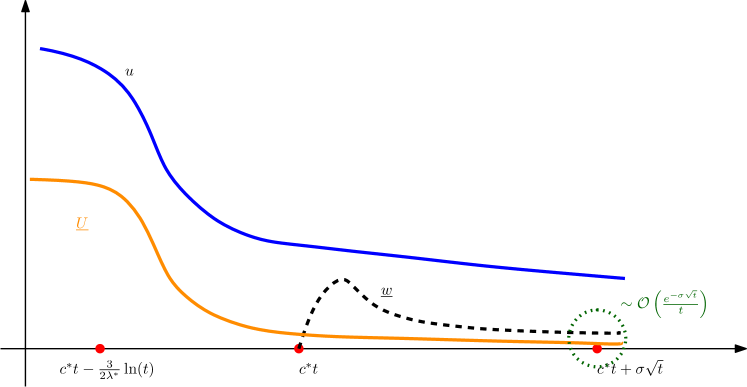
Figure 2: A sketch of the sub-solution $\underline{U}$, the solution $u$ of the Fisher-KPP problem, and of the solution of the linearized problem with the Dirichlet boundary condition at $x=c^{*}t$.

5 The proof of Proposition 4.3

In this section, we prove Proposition 4.3. The proof of the upper bound in (4.25) is easier than for the lower bound, and this is what we will do first. Essentially, the remainder of the paper will then be devoted to the proof of the lower bound in (4.25).

5.1 The self-adjoint form

Our first step is to re-write (4.23) in a self-adjoint form. Let us set

$$\mu=a(Q^{*})^{2},~{}~{}a=\Big{(}\frac{1}{|\Theta|}\int_{\Theta}(Q^{*})^{2}d\theta\Big{)}^{-1}.$$ (5.1)

Then we have an identity

$$Dp_{xx}+\Delta_{\theta}p+\frac{2}{Q^{*}}\nabla_{\theta}Q^{*}\cdot\nabla_{\theta}p=\frac{1}{\mu}\Big{[}\left(D\mu p_{x}\right)_{x}+\nabla_{\theta}\cdot(\mu\nabla_{\theta}p)\Big{]}.$$ (5.2)

In order to re-write the spatial drift term in the right side of (4.23), we look for a corrector $\beta$ that satisfies

$$\Delta_{\theta}\beta=2\lambda^{*}D+A-r\quad\hbox{ in $\Theta$},$$ (5.3)

$$\dfrac{\partial{\beta}}{\partial{\nu_{\theta}}}=0\hbox{ on $\partial\Theta$},$$

with some $r\in{\mathbb{R}}$. The solvability condition for (5.3) is

$$r=\int_{\Theta}[2\lambda^{*}D(\theta)+A(\theta)]\mu(\theta)\frac{d\theta}{|\Theta|}=a\int_{\Theta}[2\lambda^{*}D(\theta)+A(\theta)](Q^{*}(\theta))^{2}\frac{d\theta}{|\Theta|}=c^{*}.$$ (5.4)

We used (4.17) and (5.1) in the last step above. Thus, (4.23) can be recast as

$$(1-\omega)\mu p_{\tau}=\mathcal{L}p,$$ (5.5)

with the operator ${\cal L}$

$${\cal L}p=\left(D\mu p_{x}\right)_{x}+\nabla_{\theta}\cdot(\mu\nabla_{\theta}p)-\left(\Delta_{\theta}\beta+{c^{*}}\right)p_{x}.$$ (5.6)

Note that the average of the advection term in $x$ in (5.6) equals to $c^{*}$.

We now state a lemma regarding almost-linear solutions to (5.5) and its adjoint. The latter will be crucial in the proof of the upper bound for $p$. The former will be required later. We denote by ${\cal L}^{*}$ the formal adjoint of the operator ${\cal L}$ with respect to the Lebesgue measure, and set

$$\mathcal{C}_{\tau}=\left[c^{*}\tau,+\infty\right)\times\Theta,$$

Lemma 5.1.

There exist functions $\zeta$ and $f$ solving

$$\left\{\begin{array}[]{ll}\mu\partial_{\tau}\zeta=\mathcal{L}\zeta,&~{}\hbox{ on $\mathcal{C}_{\tau}$,}\vskip 6.0pt plus 2.0pt minus 2.0pt\\ \dfrac{\partial{\zeta}}{\partial{\nu_{\theta}}}=0,&\hbox{ on $\partial\Theta$},\vskip 6.0pt plus 2.0pt minus 2.0pt\\ \zeta(\tau,c^{*}\tau,\cdot)=0,\end{array}\right.~{}~{}\text{ and }~{}~{}\begin{array}[]{ll}\mu\partial_{\tau}f=-\mathcal{L}^{*}f,&~{}\hbox{ on $\mathcal{C}_{\tau}$,}\vskip 6.0pt plus 2.0pt minus 2.0pt\\ \dfrac{\partial{f}}{\partial{\nu_{\theta}}}=0&\hbox{ on $\partial\Theta$},\vskip 6.0pt plus 2.0pt minus 2.0pt\\ f(\tau,c^{*}\tau,\cdot)=0,\end{array}$$ (5.7)

such that $f_{\tau},\zeta_{\tau}\leq 0$. Moreover, there exists a constant $C>0$ such that all $x\geq c^{*}\tau$,

$$C^{-1}\left(x-c^{*}\tau\right)\leq\zeta(t,x,\theta),f(t,x,\theta)\leq C\left(x-c^{*}\tau\right),$$

and $|\partial_{\tau}f|,|\partial_{\tau}\zeta|\leq C$.

We omit the proof as it is very close to [21].

5.2 The proof of the upper bound

We now prove the upper bound in (4.25), namely, there exists a positive constant such that

$$p(\tau,x,\theta)\leq\frac{C_{0}(x-c^{*}\tau)}{(\tau+1)^{3/2}},$$ (5.8)

for all $\tau>0$, $x>c^{*}t$ and $\theta\in\Theta$. We use a standard strategy: a Nash-type inequality is used to obtain the $L^{2}$ decay in terms of the $L^{1}$ norm, and then the uniform decay follows by a duality argument.

We first derive an $L^{1}-L^{2}$ bound. Using (5.5)-(5.6), integrating by parts gives that for any $\tau>0$, we have

$$\frac{1-\omega}{2}\frac{d}{d\tau}\int_{\mathcal{C}_{\tau}}\mu(\theta)p(\tau,x,\theta)^{2}dxd\theta=-\int_{\mathcal{C}_{\tau}}\mu(\theta)\left[D(\theta)p_{x}(\tau,x,\theta)^{2}+|\nabla_{\theta}p(\tau,x,\theta)|^{2}\right]dxd\theta.$$ (5.9)

The dissipation in the right side may be estimated using a Nash type inequality for half-cylinders of the form $\Omega=[0,\infty)\times\Theta$, with $\Theta\subset{\mathbb{R}}^{d}$, for functions such that $\phi(0,\cdot)\equiv 0$:

$$\|\nabla\phi\|_{2}^{2}\geq C\left(1+\left(\frac{\|\phi\|_{2}}{\|x\phi\|_{1}}\right)^{\frac{10d}{3(3+d)}}\right)^{-1}{\|\phi\|_{2}^{2}\left(\frac{\|\phi\|_{2}}{\|x\phi\|_{1}}\right)^{\frac{4}{3}}}.$$ (5.10)

The proof of the one-dimensional version of (5.10) can be found in [21]. We describe the required modifications for $d>1$ in Section 5.8. This gives:

$$\int_{\mathcal{C}_{\tau}}\mu(\theta)\left[D(\theta)p_{x}(\tau,x,\theta)^{2}+|\nabla_{\theta}p(\tau,x,\theta)|^{2}\right]dxd\theta\geq CI_{2}(\tau)\Big{(}1+\left(\frac{I_{2}(\tau)^{1/2}}{I_{1}(\tau)}\right)^{\frac{10d}{3(3+d)}}\Big{)}^{-1}\left(\frac{I_{2}(\tau)^{1/2}}{I_{1}(\tau)}\right)^{\frac{4}{3}}.$$ (5.11)

Here, we have defined

$$\begin{split}&I_{1}(\tau):=\int_{\mathcal{C}_{\tau}}\mu(\theta)(x-c^{*}\tau)p(\tau,x,\theta)dxd\theta,~{}~{}\text{ and},\\ &I_{2}(\tau):=\int_{\mathcal{C}_{\tau}}\mu(\theta)p(\tau,x,\theta)^{2}dxd\theta.\end{split}$$

We point out that we used in (5.11) that $\mu$ is bounded uniformly away from $0$ and $\infty$.

Next, we look at

$$I(\tau):{=}\int_{\mathcal{C}_{\tau}}\mu(\theta)f(\tau,x,\theta)p(\tau,x,\theta)dxd\theta,$$

with $f$ as in (5.7). If $\omega\equiv 0$, then $I(\tau)$ is a conserved quantity. In general, following the proof of [21, Lemma 5.4], one can show that there exists a constant $C>0$ such that

$$C^{-1}I(0)\leq I(\tau)\leq C\left(\int_{\mathcal{C}_{0}}p_{0}dxd\theta+I(0)\right).$$ (5.12)

Using Lemma 5.1, we see that $I(\tau)$ and $I_{1}(\tau)$ are comparable:

$$\frac{1}{C}\int_{\mathcal{C}_{\tau}}\mu(\theta)f(\tau,x,\theta)p(\tau,x,\theta)dxd\theta\leq I_{1}(\tau)\leq C\int_{\mathcal{C}_{\tau}}\mu(\theta)f(\tau,x,\theta)p(\tau,x,\theta)dxd\theta.$$

As a consequence, we have

$$C^{-2}I_{1}(0)\leq C^{-1}I_{1}(\tau)\leq N:=\left(\int_{\mathcal{C}_{0}}p_{0}dxd\theta+I_{1}(0)\right).$$ (5.13)

Using (5.13) together with (5.9) and (5.11), we obtain

$$\left(\frac{I_{1}(\tau)^{4/3}}{I_{2}(\tau)^{5/3}}+\frac{I_{1}(\tau)^{(4-2d)/(3+d)}}{I_{2}(\tau)^{5/(3+d)}}\right)I_{2}^{\prime}(\tau)\leq-\frac{1}{C(1-\omega(\tau))}.$$ (5.14)

An elementary argument, starting with this differential inequality, using the decay assumptions on $\omega$ and (5.13), gives an upper bound

$$I_{2}(\tau)\leq\frac{CN^{2}}{(\tau+1)^{3/2}},$$ (5.15)

regardless of the cross-section dimension $d\geq 1$. In other words, we have the bound

$$\|p(\tau,\cdot)\|_{L^{2}\left(\mathcal{C}_{\tau}\right)}\leq\frac{C}{(\tau+1)^{3/4}}\int_{{\mathcal{C}}_{0}}(1+x)|p_{0}(x,\theta)|dxd\theta.$$ (5.16)

We may now apply the standard duality argument. Let $S_{\tau}$ be the solution operator mapping $p_{0}$ to $p(\tau,\cdot)$. The bound (5.15) applies that $S_{\tau}^{*}$ satisfies

$$|S_{\tau}^{*}p_{0}|\leq\frac{C(1+x-c^{*}\tau)}{(\tau+1)^{3/4}}\|p_{0}\|_{L^{2}\left(\mathcal{C}_{0}\right)}.$$ (5.17)

However, $S_{\tau}^{*}$ is the solution operator for a parabolic equation of the same type, except for the reverse drift direction, thus it also obeys the bound (5.16), and hence $S_{\tau}$ itself obeys (5.17) as well. Decomposing $S_{\tau}=S_{\tau/2}\circ S_{\tau/2}$ and applying the bounds (5.16) and (5.17) separately, we get

$$|p(\tau,x,\theta)|\leq\frac{C(1+x-c^{*}\tau)}{(\tau+1)^{3/2}}\int_{\mathcal{C}_{0}}(1+x)p_{0}(x,\theta)dxd\theta.$$ (5.18)

This proves (5.8) for $x>c^{*}\tau+1$. However, as $p(\tau,c^{*}\tau,\cdot)=0$, using the parabolic regularity for $x\in(c^{*}\tau,c^{*}\tau+1)$, we obtain the upper bound (5.8) for all $x>c^{*}\tau$. $\Box$

5.3 The lower bound for $p$

We now prove the lower bound on $p$ in Proposition 4.3, namely, there exists a positive constant such that

$$p(\tau,x,\theta)\geq\frac{(x-c^{*}\tau)}{C_{0}(\tau+1)^{3/2}},$$ (5.19)

for all $\tau>0$, $x>c^{*}t$ and $\theta\in\Theta$.

Approximate solutions

For the proof of Proposition 4.3 will make use of approximate solutions of our problem that satisfy the bounds claimed in this Proposition. Let $Q_{\lambda}$ be the eigenfunction in (4.1), and set

$$\chi=-\frac{1}{Q_{\lambda}}\frac{\partial Q_{\lambda}}{\partial\lambda}\Big{|}_{\lambda=\lambda^{*}},$$ (5.20)

and

$$\overline{D}:{=}\left(\int_{\Theta}\left(D+c^{*}\chi-2\lambda^{*}D\chi-A\chi\right)(Q^{*})^{2}d\theta\right)\left(\int_{\Theta}(Q^{*})^{2}d\theta\right)^{-1}.$$ (5.21)

To see that $\overline{D}>0$, we differentiate (4.18) in $\lambda$ to obtain

$$\int_{\Theta}\left[2Q\dfrac{\partial{Q}}{\partial{\lambda}}\left(c^{\prime}(\lambda)\lambda+c(\lambda)-2\lambda D-A\right)+Q^{2}\left(c^{\prime\prime}(\lambda)\lambda+2c^{\prime}(\lambda)-2D-A\right)\right]d\theta=0.$$ (5.22)

Evaluating (5.22) at $\lambda=\lambda^{*}$, we obtain, as $c^{\prime}(\lambda^{*})=0$:

$$0=\int_{\Theta}\left[-2(Q^{*})^{2}\chi\left(c^{*}-2\lambda^{*}D-A\right)+(Q^{*})^{2}\left(c^{\prime\prime}(\lambda)\lambda-2D-A\right)\right]d\theta.$$

Now, (5.21) and (4.18) show that this is

$$c^{\prime\prime}(\lambda^{*})\lambda^{*}\int_{\Theta}(Q^{*})^{2}d\theta=2\overline{D}\int_{\Theta}(Q^{*})^{2}d\theta.$$

Since $c^{\prime\prime}(\lambda^{*})>0$ by Proposition 4.2, we conclude that $\overline{D}>0$.

The approximate solutions are described by the following analogue of [21, Proposition 5.2].

Proposition 5.2.

Let $\overline{\chi}\in\mathbb{R}$, then there is a function $S(\tau,x,\theta)$ such that, for any $\sigma>0$,

$$(1-\omega)\frac{\partial S}{\partial\tau}-DS_{xx}-\Delta_{\theta}S+\left(2\lambda D+A\right)S_{x}-\frac{2}{Q^{*}}\nabla_{\theta}{Q^{*}}\cdot\nabla_{\theta}S=O(\tau^{-3})$$ (5.23)

and

$$\left|S(\tau,x,\cdot)-\frac{x-c^{*}\tau+\chi+\overline{\chi}}{\tau^{3/2}}e^{-\frac{(x-c^{*}\tau)^{2}}{4\overline{D}\tau}}\right|\leq C\tau^{-3/2}\left(\frac{x-c^{*}\tau}{\sqrt{\tau}}\right)^{2}+O(\tau^{-2}),$$ (5.24)

for all $x\in[c^{*}\tau,c^{*}\tau+\sigma\sqrt{\tau}]$. The constant $C$ depends on $\sigma$.

The approximate solutions do approximate true solutions on $[c^{*}\tau,c^{*}\tau+\sigma\sqrt{\tau}]$, as seen from the following.

Proposition 5.3.

Fix $\sigma>0$, and let $S$ be as in Proposition 5.2. Suppose that $\xi$ satisfies for $\tau>0$,

$$\left\{\begin{array}[]{ll}(1-\omega)\xi_{\tau}=D\xi_{xx}+\Delta_{\theta}\xi-\left(2\lambda^{*}D+A\right)\xi_{x}+\frac{2}{Q^{*}}\nabla Q^{*}\cdot\nabla\xi,&\qquad x\in[c^{*}\tau,c^{*}\tau+\sigma\sqrt{\tau}],\vskip 6.0pt plus 2.0pt minus 2.0pt\\ \xi(\tau,c^{*}\tau,\cdot)=S(\tau,c^{*}\tau,\cdot),&\vskip 6.0pt plus 2.0pt minus 2.0pt\\ \xi(\tau,c^{*}\tau+\sigma\sqrt{\tau},\cdot)=S(\tau,c^{*}\tau+\sigma\sqrt{\tau},\cdot).\end{array}\right.$$ (5.25)

Then there is a positive constant $\tau_{0}$ such that, if $\tau\geq\tau_{0}$ and $x-c^{*}\tau\in(0,\sigma\sqrt{\tau})$, then

$$|\left(\xi-S\right)(\tau,x,\cdot)|\leq\frac{C}{\tau^{3/2}}.$$

The proof of Proposition 5.3 is a relatively straightforward energy estimate of the difference $\xi-S$ that can be obtained almost exactly as in [21, Proposition 5.3].

The size of the solution at distance $O(\sqrt{\tau})$

Another key step is to establish the magnitude of $p$ at distances of the order $O(\sqrt{\tau})$ from $x=c^{*}\tau$. With the following proposition, we control $p$ at the endpoints of the interval $[c^{*}\tau,c^{*}\tau+\sigma\sqrt{\tau}]$. Then, the previous propositions allow us to control $p$ in the remainder of the interval as $S$ approximates $p$.

Proposition 5.4.

Let $p$ be as in Proposition 4.3. There are constants $\sigma>0$ and $C_{0}>0$ so that

$$\frac{1}{C_{0}\tau}\leq p(\tau,c^{*}\tau+\sigma\sqrt{\tau})\leq\frac{C_{0}}{\tau}$$ (5.26)

whenever $\tau\geq 1$.

Sketch of the proof of Proposition 4.3

We now outline how to combine Propositions 5.2, 5.3 and 5.4 to obtain the lower bound in Proposition 4.3. Proposition 5.4 controls $p$ at the point $c^{*}\tau+\sigma\sqrt{\tau}$ in a way consistent with (4.25). On the other hand, by choosing $\overline{\chi}=-(1+\|\chi\|_{\infty})$ in Proposition 5.2, the combination of Propositions 5.2 and 5.3 allows us to build a sub-solution $\xi^{-}$ to $p$. Then, re-applying Proposition 5.3, we see that $\xi^{-}$ satisfies the bounds in (4.25) except on a finite interval $[c^{*}\tau,c^{*}\tau+x_{0}]$, for some $x_{0}$. By the comparison principle, we may then transfer these bounds to $p$ and use parabolic regularity to remove the condition on $x_{0}$, finishing the proof of the claim. Thus, it remains to prove Propositions 5.2 and 5.4, which is done in the rest of this paper.

5.4 The proof of Proposition 5.2

Our strategy is the same as in [21, Proposition 5.2], though the details are different, so we include a sketch of the proof for reader’s convenience. We begin with the multi-scale expansion

$$S(\tau,x,\theta)=\frac{1}{\tau}\left(S^{0}(z)+\frac{S^{1}(z,\theta)}{\sqrt{\tau}}+\frac{S^{2}(z,\theta)}{\tau}+\frac{S^{3}(z,\theta)}{\tau^{3/2}}\right),~{}~{}z=\frac{x-c^{*}\tau}{\sqrt{\tau}}.$$

Plugging this into the left hand side of (5.23), we obtain the equation

$$\begin{split}&\frac{(1-\omega)}{\tau}\left[-\frac{S^{0}}{\tau}-\frac{3S^{1}}{2\tau^{3/2}}-\frac{2S^{2}}{\tau^{2}}-\frac{5S^{3}}{2\tau^{5/2}}\right]+\frac{(1-\omega)}{\tau}\left[-c^{*}\frac{S^{0}_{z}}{\tau^{1/2}}-c^{*}\frac{S^{1}_{z}}{\tau}-c^{*}\frac{S^{2}_{z}}{\tau^{3/2}}-c^{*}\frac{S^{3}_{z}}{\tau^{2}}\right]\\ &+\frac{(1-\omega)}{\tau}\left[-\frac{z}{2}\frac{S^{0}_{z}}{\tau}-\frac{z}{2}\frac{S^{1}_{z}}{\tau^{3/2}}-\frac{z}{2}\frac{S^{2}_{z}}{\tau^{2}}-\frac{z}{2}\frac{S^{3}_{z}}{\tau^{5/2}}\right]+\frac{D}{\tau}\left[-\frac{S^{0}_{zz}}{\tau}-\frac{S^{1}_{zz}}{\tau^{3/2}}-\frac{S^{2}_{zz}}{\tau^{2}}-\frac{S^{3}_{zz}}{\tau^{5/2}}\right]\\ &+\frac{1}{\tau}\left[\frac{LS^{1}}{\tau^{1/2}}+\frac{LS^{2}}{\tau}+\frac{LS^{3}}{\tau^{3/2}}\right]+\frac{\left(2\lambda^{*}D+A\right)}{\tau}\left[\frac{S^{0}_{z}}{\sqrt{\tau}}+\frac{S^{1}_{z}}{\tau}+\frac{S^{2}_{z}}{\tau^{3/2}}+\frac{S^{3}_{z}}{\tau^{2}}\right]=0.\end{split}$$ (5.27)

Here, we have defined the operator

$$L=\Delta_{\theta}+\frac{2}{Q^{*}}\nabla_{\theta}Q^{*}\cdot\nabla_{\theta}.$$

Grouping the terms of order $\tau^{-3/2}$ in (5.27), we obtain

$$LS^{1}=\left(c^{*}-2\lambda^{*}D-A\right)S^{0}_{z}.$$ (5.28)

It is easy to verify that (5.28) has a solution of the form

$$S^{1}=\chi_{0}S^{0}_{z}+\phi_{1},~{}~{}~{}\chi_{0}=\chi+\overline{\chi},$$ (5.29)

where $\phi_{1}$ only depends on $z$. The terms of order $\tau^{-2}$ in (5.27) give

$$-S^{0}-c^{*}S^{1}_{z}-\frac{z}{2}S^{0}_{z}-DS^{0}_{zz}+LS^{2}+2\lambda DS^{1}_{z}+AS^{1}_{z}=0.$$ (5.30)

Using expression (5.29) for $S^{1}$, multiplying (5.30) by $(Q^{*})^{2}$ and integrating in $\theta$, we obtain

$$S^{0}+\frac{z}{2}S^{0}_{z}+\overline{D}S^{0}_{zz}=0$$ (5.31)

with $\overline{D}$ as in (5.21), so that

$$S^{0}(z)=z\exp\left\{-\frac{z^{2}}{4\overline{D}}\right\}.$$ (5.32)

With this in hand, we return to (5.30) that we write as

$$LS^{2}=(c^{*}-2\lambda D+A)(S^{1})_{z}+(D+c^{*}\chi_{0}-2\lambda^{*}D\chi_{0}+A\chi_{0}-\overline{D})S^{0}_{zz}.$$ (5.33)

One solution of (5.33) is

$$S^{2}(z,\theta)=\chi_{0}(\theta)(\phi_{1})_{z}(z)+\hat{S}^{2}(\theta)S^{0}_{zz}(z),$$

where $\hat{S}^{2}(\theta)$ is any solution to

$$L\hat{S}^{2}=D+c^{*}\chi_{0}-2\lambda^{*}D\chi_{0}+A\chi_{0}-\overline{D},$$ (5.34)

with the Neumann boundary conditions. The definition of $\overline{D}$ ensures that solution of (5.34) exists.

Continuing, we examine the terms of order $\tau^{-5/2}$ to obtain

$$-\frac{3}{2}S^{1}+\overline{\omega}c^{*}S^{0}_{z}-c^{*}S^{2}_{z}-\frac{z}{2}S^{1}_{z}-DS^{1}_{zz}+2\lambda DS^{2}_{z}+LS^{3}+AS^{2}_{z}=0.$$ (5.35)

Here, we replaced $\omega$ by $\overline{\omega}/\tau$ at the expense of lower order terms which we may absorb into the $O(\tau^{-3})$ term in (5.23). Multiplying by $(Q^{*})^{2}$ and integrating over $\theta$ yields the solvability condition for $S^{3}$:

$$-\frac{3}{2}\phi_{1}-\frac{z}{2}\left(\phi_{1}\right)_{z}-\overline{D}(\phi_{1})_{zz}=\left(3\beta_{1}-\overline{\omega}c^{*}\right)S^{0}_{z}+z\beta_{1}S^{0}_{zz}+\beta_{2}S^{0}_{zzz}.$$ (5.36)

Here, we have defined

$$\beta_{1}:{=}\frac{1}{2}\frac{\int_{\Theta}\chi_{0}(Q^{*})^{2}d\theta}{\int_{\Theta}(Q^{*})^{2}d\theta},~{}~{}~{}\beta_{2}:{=}\frac{\int_{\Theta}(c^{*}\hat{S}^{2}-2\lambda D\hat{S}^{2}-A\hat{S}^{2}+D)(Q^{*})^{2}d\theta}{\int_{\Theta}(Q^{*})^{2}d\theta}.$$

We may now choose $\phi_{1}$ to be the unique solution to (5.36) with $\phi_{1}(0)=0$ and $(\phi_{1})_{z}(0)=0$. Since $S^{0}$ and its derivatives are bounded, there exists a constant $C$ such that $|\phi_{1}(z)|\leq Cz^{2}$ for all $|z|\leq\sigma$. For the sake of clarity, we write $\phi_{1}=z^{2}\overline{\phi}$, with a bounded function $\overline{\phi}$.

Finally, grouping the $\tau^{-3}$ terms together and setting them to zero, we get an equation for $S^{3}$. It follows from the elliptic regularity theory that, for $z\leq\sigma$, $S^{3}$ is uniformly bounded. To summarize, we have found an approximate solution, in the sense that (5.23) holds, of the form

$$S=\frac{x-c^{*}\tau}{\tau^{3/2}}e^{-\frac{(x-c^{*}\tau)^{2}}{4\overline{D}\tau}}+\chi_{0}\frac{1-\frac{z^{2}}{4\overline{D}\tau}}{\tau^{3/2}}e^{-\frac{(x-c^{*}\tau)^{2}}{4\overline{D}\tau}}+\frac{x-c^{*}\tau}{\tau^{5/2}}\overline{\phi}(z)+\frac{S^{2}}{\tau^{2}}+\frac{S^{3}}{\tau^{5/2}}.$$ (5.37)

It also clearly satisfies the condition (5.24). This concludes the proof. $\Box$

5.5 Understanding $p$ at $x-c^{*}\tau\sim O(\sqrt{\tau})$: the proof of Proposition 5.4

The lower bound in (5.26) is a consequence of an integral bound.

Lemma 5.5.

There exists a time $T_{0}>0$ and constants $c_{0}$, $B$, and $N$, depending only on the initial data, such that for any $\tau>T_{0}$ there exists a set $I_{\tau}\subset[c^{*}\tau+N^{-1}\sqrt{\tau},c^{*}t+N\sqrt{\tau}]$ with $|I_{\tau}|\geq B\sqrt{\tau}$ and with

$$\frac{1}{c_{0}\tau}\leq\int_{\Theta}p(\tau,x,\eta)d\eta.$$ (5.38)

Proposition 5.4 follows from Lemma 5.5 and a standard heat kernel bound. Indeed, let us assume that $\omega=0$, as we may otherwise apply the time change

$$d\tau^{\prime}=\frac{d\tau}{1-\omega(\tau)}.$$

Let $\Gamma$ be the heat kernel for (5.5)-(5.6) with the Dirichlet boundary condition at $x=c^{*}t$. That is, the solution of

$$\mu\psi_{\tau}=\left(D\mu\psi_{x}\right)_{x}+\nabla_{\theta}\cdot(\mu\nabla_{\theta}\psi)-\left(\Delta_{\theta}\beta+{c^{*}}\right)\psi_{x},~{}~{}\tau>s,~{}x>c^{*}\tau,~{}\theta\in\Theta,$$

$$\dfrac{\partial{\psi}}{\partial{\nu_{\theta}}}=0,\hbox{ on $\partial\Theta$},$$ (5.39)

$$\psi(\tau,c^{*}\tau,\cdot)=0,$$

$$\psi(s,\cdot)=\bar{\psi},$$

can be written as

$$\psi(\tau,x,\theta)=\int_{{\cal C}_{s}}\Gamma(\tau,x,\theta,s,y,\eta)\bar{\psi}(y,\eta)\mu(\eta)dyd\eta.$$ (5.40)

As in [21], one can show the following, starting with the standard heat kernel bound in a cylinder. Set $\Phi(s)=s$ for $s\in[0,1]$ and $\Phi(s)=\sqrt{s}$ for $s>1$, then for all $\delta>0$, there exists a constant $K$ such that

$$\Gamma(\tau,x,\theta,s,y,\eta)\geq\frac{1}{K\Phi(\tau-s)}\exp\left\{-K\frac{|x-y|^{2}+|\theta-\eta|^{2}}{\Phi(\tau-s)}\right\}$$ (5.41)

whenever $R>0$, $\tau\in(s,s+R^{2}]$, and $x,y\in(c^{*}\tau+\xi-\delta R,c^{*}\tau+\xi+\delta R)$. A straightforward computation using (5.40) going from the time $s=\tau/2$ to $\tau$ shows that the integral bound (5.38), combined with the pointwise lower bound (5.41) on the heat kernel, lead to a pointwise lower bound on $p$ in Proposition 5.4. $\Box$

5.6 Proof of Lemma 5.5

An exponentially weighted estimate

As in [21], one may show that for all $\alpha>0$, there exists a function $\eta_{\alpha}$ that satisfies

$$\mu\partial_{\tau}\eta_{\alpha}=-\mathcal{L}^{*}\left(\mu\eta_{\alpha}\right)+\aleph(\alpha)\mu\eta_{\alpha},~{}\hbox{ on $\mathcal{C}_{\tau}$,}$$

$$\dfrac{\partial{\eta_{\alpha}}}{\partial{\nu_{\theta}}}=0\hbox{ on $\partial\Theta$,}$$

$$\eta_{\alpha}(\tau,c^{*}\tau,\cdot)=0.$$

as well as the exponential bounds

$$\frac{e^{\alpha(x-c^{*}\tau)}-e^{-\alpha(x-c^{*}\tau)}}{C\alpha}\leq\eta_{\alpha}(t,x,\theta)\leq C\frac{e^{\alpha(x-c^{*}\tau)}-e^{-\alpha(x-c^{*}\tau)}}{\alpha}.$$ (5.43)

The eigenvalue $\aleph(\alpha)$ in (5.6) behaves as

$$\aleph(\alpha)=\aleph_{0}\alpha^{2}+O(\alpha^{3}),$$ (5.44)

as $\alpha$ tends to zero, with some $\aleph_{0}>0$. Moreover, we have

$$\begin{split}&|\partial_{\tau}\eta_{\alpha}|\leq C~{}~{}\qquad\text{ for all }x\in[c^{*}\tau,c^{*}\tau+\alpha^{-1}],~{}\text{ and }\\ &|\partial_{\tau}\eta_{\alpha}|\leq C\alpha\eta_{\alpha}~{}~{}~{}\text{ for all }x\geq c^{*}\tau+\alpha^{-1}.\end{split}$$ (5.45)

With this in hand, we define

$$V_{\alpha}(\tau)=\left(1-\omega(\tau)\right)\int_{\mathcal{C}_{\tau}}\mu(\theta)\,\eta_{2\alpha}(\tau,x,\theta)\,p(\tau,x,\theta)\,q(\tau,x,\theta)\,dxd\theta.$$ (5.46)

Here, we write

$$p=q\zeta,$$ (5.47)

and $\zeta$ is as in Lemma 5.1. Lemma 5.5 is a consequence of the following estimate.

Lemma 5.6.

There is a constant $C_{0}$ depending on $p_{0}$ such that

$$V_{\tau^{-1/2}}(\tau)\leq C_{0}\tau^{-3/2}.$$ (5.48)

We first show how to conclude the proof of Lemma 5.5 from Lemma 5.6. Note that (5.48) implies

$$\left(\int_{0}^{\infty}\int_{\Theta}\frac{e^{2x/\sqrt{\tau}}-e^{-2x/\sqrt{\tau}}}{x}p(\tau,c^{*}\tau+x,\theta)^{2}dxd\theta\right)^{1/2}\leq\frac{C_{0}}{\tau},$$ (5.49)

Fix $N>0$ to be determined later, then (5.49) gives, in particular:

$$\int_{N\sqrt{\tau}}^{\infty}\int_{\Theta}xp(\tau,c^{*}\tau+x,\theta)dxd\theta=\int_{N\sqrt{\tau}}^{\infty}\int_{\Theta}\frac{e^{x/\sqrt{\tau}}}{\sqrt{x}}p(\tau,c^{*}\tau+x,\theta)e^{-x/\sqrt{\tau}}x^{3/2}dxd\theta$$

$$\leq\left(\int_{N\sqrt{\tau}}^{\infty}\int_{\Theta}\frac{e^{2x/\sqrt{\tau}}}{x}p(\tau,c^{*}\tau+x,\theta)^{2}dxd\theta\right)^{1/2}\left(\int_{N\sqrt{\tau}}^{\infty}\int_{\Theta}e^{-2x/\sqrt{\tau}}x^{3}dxd\theta\right)^{1/2}$$

$$\leq\frac{C}{\tau}\left(\int_{N\sqrt{t}}^{\infty}\int_{\Theta}e^{-2x/\sqrt{\tau}}x^{3}dxd\theta\right)^{1/2}\leq C_{0}N^{3}e^{-N/2}.$$ (5.50)

On the other hand, we also have

$$\int_{0}^{\sqrt{\tau}/N}\int_{\Theta}xp(\tau,c^{*}\tau+x,\theta)dxd\theta\leq C_{0}N^{-3}.$$

Hence, choosing $N$ sufficiently large, depending only on the initial data of $p$ and not on time, we have

$$\int_{\sqrt{\tau}/N}^{N\sqrt{\tau}}\int_{\Theta}xp(\tau,c^{*}\tau+x,\theta)dxd\theta\geq C_{0}.$$ (5.51)

Let us set

$$I_{\tau}:{=}\left\{x\in[c^{*}\tau+\sqrt{\tau}/N,c^{*}\tau+N\sqrt{\tau}]:\int_{\Theta}p(\tau,x,\eta)d\eta\geq\frac{C_{0}}{4N^{2}\tau}\right\}.$$

Then, (5.51) implies

$$\frac{3C_{0}}{4}\leq\int_{I_{\tau}}\int_{\Theta}(x-c^{*}\tau)p(\tau,x,\theta)dxd\theta\leq\int_{I_{\tau}}\int_{\Theta}\frac{C_{0}(x-c^{*}\tau)^{2}}{\tau^{3/2}}dxd\theta\leq|I_{\tau}|\frac{C_{0}N^{2}}{\tau^{1/2}},$$

and the proof of Lemma 5.5 is complete. $\Box$

5.7 The proof of Lemma 5.6

Throughout this section we use the assumption that $\tau\leq\alpha^{-2}$. The proof relies on two observations. First, we have the following energy-dissipation inequality for $V_{\alpha}$:

$$V_{\alpha}^{\prime}(\tau)\leq\displaystyle\left(\aleph(2\alpha)-\frac{\omega^{\prime}(\tau)}{1-\omega(\tau)}+C\alpha\omega(\tau)\right)V_{\alpha}(\tau)-2D_{\alpha}(\tau)+\frac{C_{0}}{(\tau+1)^{5/2}},$$ (5.52)

with the dissipation

$$D_{\alpha}=\int_{\mathcal{C}_{\tau}}\mu(\theta)\eta_{2\alpha}(\tau,x,\theta)\zeta(\tau,x,\theta)\left(D(\theta)|q_{x}(\tau,x,\theta)|^{2}+|q_{\theta}(\tau,x,\theta)|^{2}\right)dxd\theta.$$ (5.53)

Recall that the function $\zeta$ is defined in Lemma 5.1, and $q$ is as in (5.47). Since this computation is quite involved, we delay it for the moment.

The second observation is that the dissipation $D_{\alpha}$ may be related to $V_{\alpha}$ by the inequality

$$D_{\alpha}\geq\frac{1}{C_{0}}V_{\alpha}^{5/3}$$ (5.54)

where $C_{0}$ is a constant depending only on $p_{0}$ and $\tau\in[0,T]$. We also delay the proof of (5.54).

The combination of (5.52) and (5.54) yields the differential inequality

$$V_{\alpha}^{\prime}\leq\left(\aleph(2\alpha)-\frac{\omega^{\prime}}{1-\omega}+\frac{C\alpha}{\tau+1}\right)V_{\alpha}-\frac{1}{C_{0}}V_{\alpha}^{5/3}+\frac{C_{0}}{(\tau+1)^{5/2}}.$$ (5.55)

Let us define

$$Z(\tau)=(\tau+1)^{3/2}V_{\alpha}\exp(-\Phi(\tau)),~{}~{}\Phi(\tau)=\aleph(2\alpha)\tau+\log(1-\omega(\tau))+C\alpha\log(\tau+1).$$

Note that, as $\tau\leq\alpha^{-2}$, we know, due to the asymptotics (5.44) for $\aleph(2\alpha)$, that

$$|\Phi(s)|\leq C 0\leq s\leq\tau$$ for all , (5.56)

with a constant $C>0$ that is independent of $\alpha>0$ sufficiently small. Thus, (5.48) would follow if we show that that $Z$ is uniformly bounded above. However, it follows from (5.55) and (5.56) that $Z$ satisfies

$$Z^{\prime}\leq C\frac{Z}{\tau+1}+\frac{C_{0}}{\tau+1}-\frac{1}{C_{0}(\tau+1)}Z^{5/3}.$$

This implies

$$Z^{5/3}\leq\max\left\{C\left(Z+C_{0}\right),Z(0)^{5/3}\right\}.$$

Hence, $Z$ is bounded uniformly above. Thus, to finish the proof of Lemma 5.6, it only remains to show (5.52) and (5.54).

Proof of the differential inequality (5.52) for $V_{\alpha}$

Differentiating $V_{\alpha}$, we obtain

$$V_{\alpha}^{\prime}=\displaystyle-\frac{\omega^{\prime}}{1-\omega}V_{\alpha}+\left(1-\omega\right)\int_{\mathcal{C}_{\tau}}\mu\left[\left(\partial_{\tau}\eta_{2\alpha}\right)pq+\eta_{2\alpha}p_{\tau}q+\eta_{2\alpha}pq_{\tau}\right]dxd\theta.$$ (5.57)

Let us re-write the integral in (5.57). By the definition of $\eta_{2\alpha}$, we have

$$\begin{split}\left(1-\omega\right)\int_{\mathcal{C}_{\tau}}\mu\left(\partial_{\tau}\eta_{2\alpha}\right)pq\,dxd\theta&=\left(1-\omega\right)\int_{\mathcal{C}_{\tau}}\left[-\mathcal{L}^{*}\left(\mu\eta_{2\alpha}\right)+\aleph(2\alpha)\mu\eta_{\alpha}\right]pq\,dxd\theta,\\ &=\displaystyle-\left(1-\omega\right)\int_{\mathcal{C}_{\tau}}\mu\eta_{2\alpha}\mathcal{L}(pq)\,dxd\theta+\aleph(2\alpha)V_{\alpha}.\end{split}$$

Using equation (4.23) for $p$, we deduce

$$V_{\alpha}^{\prime}=\displaystyle\left\{\aleph(2\alpha)-\frac{\omega^{\prime}}{1-\omega}\right\}V_{\alpha}+\int_{\mathcal{C}_{\tau}}\mu\eta_{2\alpha}\left[-\left(1-\omega(\tau)\right)\mathcal{L}(pq)+\mathcal{L}(p)q+(1-\omega)pq_{\tau}\right]dxd\theta.$$ (5.58)

The last integral requires a bit of work. Note that

$$\mathcal{L}(pq)=p\mathcal{L}(q)+q\mathcal{L}(p)+2Dp_{x}q_{x}+2p_{\theta}q_{\theta},$$

and

$$(1-\omega)q_{\tau}=\displaystyle\mathcal{L}(q)+\frac{q}{\zeta}\left(\mathcal{L}\left(\zeta\right)-\left(1-\omega\right)\zeta_{\tau}\right)+2D\frac{\zeta_{x}}{\zeta}q_{x}+2\frac{\zeta_{\theta}}{\zeta}q_{\theta},$$

$$~{}~{}~{}~{}~{}~{}~{}~{}~{}~{}~{}~{}~{}~{}~{}~{}=\displaystyle\mathcal{L}(q)+\frac{q}{\zeta}\left(\mathcal{L}\left(\zeta\right)-\zeta_{\tau}\right)+\omega\frac{\zeta_{\tau}}{\zeta}q+2D\frac{\zeta_{x}}{\zeta}q_{x}+2\frac{\zeta_{\theta}}{\zeta}q_{\theta}.$$

Thus, we may re-write (5.58) as

$$\begin{split}V_{\alpha}^{\prime}&=\displaystyle\left(\aleph(2\alpha)-\frac{\omega^{\prime}}{1-\omega}\right)V_{\alpha}+\omega\displaystyle\int_{\mathcal{C}_{\tau}}\mu\eta_{2\alpha}\mathcal{L}(pq)dxd\theta+\omega\int_{\mathcal{C}_{\tau}}\mu\eta_{2\alpha}pq\frac{\zeta_{\tau}}{\zeta}dxd\theta\\ &\qquad-2\displaystyle\int_{\mathcal{C}_{\tau}}\mu\eta_{2\alpha}(Dp_{x}q_{x}+p_{\theta}q_{\theta})dxd\theta+2\int_{\mathcal{C}_{\tau}}\mu\eta_{2\alpha}p\left(D\frac{\zeta_{x}}{\zeta}q_{x}+\frac{\zeta_{\theta}}{\zeta}q_{\theta}\right)dxd\theta.\end{split}$$

The last two terms in the right side can be combined as

$$\begin{split}&-2\displaystyle\int_{\mathcal{C}_{\tau}}\mu\eta_{2\alpha}(Dp_{x}q_{x}+\alpha p_{\theta}q_{\theta})\,dxd\theta+2\displaystyle\int_{\mathcal{C}_{\tau}}\mu\eta_{2\alpha}\left(D\frac{\zeta_{x}}{\zeta}q_{x}+\frac{\zeta_{\theta}}{\zeta}q_{\theta}\right)p\,dxd\theta\\ &\quad=-2\displaystyle\int_{\mathcal{C}_{\tau}}\mu\eta_{2\alpha}\left(D\left(p_{x}-\frac{\zeta_{x}}{\zeta}p\right)q_{x}+\left(p_{\theta}-\frac{\zeta_{\theta}}{\zeta}p\right)q_{\theta}\right)dxd\theta\\ &\quad=-2\displaystyle\int_{\mathcal{C}_{\tau}}\mu\eta_{2\alpha}\zeta\left(D|q_{x}|^{2}+|q_{\theta}|^{2}\right)dxd\theta=-2D_{\alpha},\end{split}$$

hence

$$V_{\alpha}^{\prime}=\displaystyle\left(\aleph(2\alpha)-\frac{\omega^{\prime}}{1-\omega}\right)V_{\alpha}-2D_{\alpha}+\omega\displaystyle\int_{\mathcal{C}_{\tau}}\mu\eta_{2\alpha}\left(\mathcal{L}(pq)+p\frac{\zeta_{\tau}}{\zeta}q\right)dxd\theta.$$ (5.59)

The estimate (5.52) will be complete after estimating the last term in the right side. We write

$$\int_{\mathcal{C}_{\tau}}\mu\eta_{2\alpha}\left(\mathcal{L}(pq)+p\frac{\zeta_{\tau}}{\zeta}q\right)dxd\theta=\int_{\mathcal{C}_{\tau}}\left(pq\mathcal{L}^{*}(\mu\eta_{2\alpha})+\mu\eta_{2\alpha}\frac{\zeta_{\tau}}{\zeta}pq\right)dxd\theta\leq\int_{\mathcal{C}_{\tau}}\mu[\partial_{\tau}\eta_{2\alpha}]pq\,dxd\theta,$$ (5.60)

as $\zeta_{\tau}\leq 0$. We use (5.45) to obtain

$$\begin{split}\left|\int_{\mathcal{C}_{\tau}}\mu\partial_{\tau}\eta_{2\alpha}pqdxd\theta\right|&\leq\left|\int_{c^{*}\tau}^{c^{*}\tau+\alpha^{-1}}\int_{\Theta}\mu\partial_{\tau}\eta_{2\alpha}pqdxd\theta\right|+\left|\int_{c^{*}\tau+\alpha^{-1}}^{\infty}\int_{\Theta}\mu\partial_{\tau}\eta_{2\alpha}pqdxd\theta\right|\\ &\leq\int_{c^{*}\tau}^{c^{*}\tau+\alpha^{-1}}\int_{\Theta}\mu pqdxd\theta+C\alpha\int_{c^{*}\tau+\alpha^{-1}}^{\infty}\int_{\Theta}\mu\eta_{2\alpha}pqdxd\theta.\end{split}$$

The second term above is $C\alpha V_{\alpha}$, as desired. For the first term, we apply the upper bound (5.8) for $p$ and the asymptotics for $\zeta$ in Lemma 5.1 to obtain

$$\int_{c^{*}\tau}^{c^{*}\tau+\alpha^{-1}}\int_{\Theta}\mu pqdxd\theta\leq\frac{C_{0}}{(\tau+1)^{3/2}}\int_{c^{*}\tau}^{c^{*}\tau+\alpha^{-1}}\int_{\Theta}pdxd\theta.$$

Integrating (5.5), we see that $\int_{\mathcal{C}_{\tau}}\mu pdxd\theta$ is non-increasing in time. Hence, we obtain that

$$\omega\int_{\mathcal{C}_{\tau}}\mu\eta_{2\alpha}\left(\mathcal{L}(pq)+p\frac{\zeta_{\tau}}{\zeta}q\right)dxd\theta\leq\frac{C_{0}}{(\tau+1)^{5/2}}+C\frac{\alpha}{\tau+1}V_{\alpha}.$$

Returning to (5.59), we obtain the desired differential inequality

$$V_{\alpha}^{\prime}=\left(\aleph(2\alpha)-\frac{\omega^{\prime}(\tau)}{1-\omega(\tau)}+C\frac{\alpha}{\tau+1}\right)V_{\alpha}-2D_{\alpha}+\frac{C_{0}}{(\tau+1)^{5/2}}.$$

Proof of the inequality (5.54) relating $V_{\alpha}$ and $D_{\alpha}$ 

It is helpful to define

$$\varphi(\tau,z,\theta)=e^{\alpha z_{3}}q(\tau,c^{*}\tau+|z|,\theta),$$

with $(z_{1},z_{2},z_{3})=z\in\mathbb{R}^{3}$, and consider the following quantities

$$\begin{split}&\hat{I}_{\alpha}:=\frac{1}{2\pi}\int_{\mathbb{R}^{3}\times\Theta}\varphi(\tau,z,\theta)dzd\theta=\int_{\mathcal{C}_{\tau}}\left(\frac{e^{\alpha(x-c^{*}\tau)}-e^{-\alpha(x-c^{*}\tau)}}{\alpha}\right)(x-c^{*}\tau)q(\tau,x,\theta)\mu\,dzd\theta,\\ &\hat{V}_{\alpha}:=\frac{1}{2\pi}\int_{\mathbb{R}^{3}\times\Theta}\varphi(\tau,z,\theta)^{2}dzd\theta=\int_{\mathcal{C}_{\tau}}\left(\frac{e^{2\alpha(x-c^{*}\tau)}-e^{-2\alpha(x-c^{*}\tau)}}{\alpha}\right)(x-c^{*}\tau)q^{2}(\tau,x,\theta)\mu\,dzd\theta,\\ &\hat{D}_{\alpha}:=\frac{1}{2\pi}\int_{\mathbb{R}^{3}\times\Theta}|\nabla\varphi(\tau,z,\theta)|^{2}dzd\theta\\ &\qquad=\int_{\mathcal{C}_{\tau}}\left(\frac{e^{2\alpha(x-c^{*}\tau)}-e^{-2\alpha(x-c^{*}\tau)}}{2\alpha}\right)(x-c^{*}\tau)(|\nabla q(\tau,x,\theta)|^{2}-\alpha^{2}q(\tau,x,\theta)^{2})\mu\,dzd\theta.\end{split}$$ (5.61)

They can be related by the following Nash-type inequality.

Proposition 5.7.

Let $\Theta\subset\mathbb{R}^{d}$ be a smooth, bounded domain, and $\Omega=\mathbb{R}^{k}\times\Theta$. There exists a constant $C$, depending only on $d$, $k$, and $|\Theta|$ such that if $\phi$ is any function in $L^{1}(\Omega)\cap H^{1}(\Omega)$ satisfying Neumann boundary conditions on the boundary $\partial\Theta$, then

$$\|\nabla\phi\|_{2}^{2}\geq C\Big{(}1+\left(\frac{\|\phi\|_{2}}{\|\phi\|_{1}}\right)^{\frac{2d(k+2)}{k(k+d)}}\Big{)}^{-1}{\|\phi\|_{2}^{2}\left(\frac{\|\phi\|_{2}}{\|\phi\|_{1}}\right)^{\frac{4}{k}}}.$$ (5.62)

Inequality (5.62) is a multi-dimensional version of a Nash-type inequality in [16], while the one-dimensional version of (5.10) is in [21]. Its proof is in Section 5.8.

We may apply Proposition 5.7 to $\phi$ in the cylinder $\mathbb{R}^{3}\times\Theta$ to obtain

$$\hat{D}_{\alpha}\geq\frac{1}{C}\frac{\hat{V}_{\alpha}^{5/3}\hat{I}_{\alpha}^{-4/3}}{1+\hat{V}_{\alpha}^{5d/(3d+9)}\hat{I}_{\alpha}^{-10d/(3d+9)}}$$ (5.63)

Using the bounds for $\zeta$ in Lemma 5.1 and the exponential bounds (5.43) for $\eta_{\alpha}$, we see that

$$C^{-1}\hat{V}_{\alpha}\leq V_{\alpha}\leq C\hat{V}_{\alpha}~{}~{}~{}\text{ and }~{}~{}~{}\hat{D}_{\alpha}\leq CD_{\alpha}.$$ (5.64)

We claim that

$$\frac{1}{C_{0}}\leq\hat{I}_{\alpha}\leq C_{0}~{}~{}~{}\text{ and }~{}~{}~{}V_{\alpha}\leq C_{0},$$ (5.65)

so that (5.63) implies

$$D_{\alpha}\geq\frac{1}{C_{0}}V_{\alpha}^{5/3},$$

which is (5.54).

To finish, we need to show that (5.65) holds. We begin with the inequality for $\hat{I}_{\alpha}$ in (5.65). Let us introduce

$$I_{\alpha}=(1-\omega)\int_{\mathcal{C}_{\tau}}\mu(\theta)\eta_{\alpha}(\tau,x,\theta)p(\tau,x,\theta)dxd\theta.$$ (5.66)

We note that

$$C^{-1}I_{\alpha}\leq\hat{I}_{\alpha}\leq CI_{\alpha},$$

by (5.43). Hence, we need only show that $I_{\alpha}$ is bounded away from infinity and zero uniformly in $\tau$ and $\alpha$ for all $\tau\leq\alpha^{-2}$. Let us differentiate $I_{\alpha}$:

$$I_{\alpha}^{\prime}=-\frac{\omega^{\prime}}{1-\omega}I_{\alpha}+(1-\omega)\int_{\mathcal{C}_{\tau}}\mu\left[p\partial_{\tau}\eta_{\alpha}+\eta_{\alpha}p_{\tau}\right]dxd\theta.$$

Using (4.23) and (5.6) allows us to rewrite the integral involving $p_{\tau}$:

$$I_{\alpha}^{\prime}(\tau)=\left(\aleph(\alpha)-\frac{\omega^{\prime}(\tau)}{1-\omega(\tau)}\right)I_{\alpha}(\tau)-\omega(\tau)\int_{\mathcal{C}_{\tau}}\mu p\partial_{\tau}\eta_{\alpha}\,dxd\theta.$$ (5.67)

The last term may be estimated as

$$\begin{split}\omega\left|\int_{\mathcal{C}_{\tau}}\mu p\partial_{\tau}\eta_{\alpha}dxd\theta\right|&\leq C\omega\int_{c^{*}\tau}^{c^{*}\tau+\alpha^{-1}}\int_{\Theta}pdxd\theta+C\omega\alpha\int_{c^{*}\tau+\alpha^{-1}}^{\infty}\int_{\Theta}p\eta_{\alpha}dxd\theta.\end{split}$$ (5.68)

The second term in (5.68) is bounded by $C(\tau+1)^{-1}\alpha I_{\alpha}$. The first requires a bit more work. First, split the integral as

$$\int_{c^{*}\tau}^{c^{*}\tau+\alpha^{-1}}\int_{\Theta}pdxd\theta=\int_{c^{*}\tau}^{c^{*}\tau+\min\{\tau^{2/3},\alpha^{-1}\}}\int_{\Theta}pdxd\theta+\int_{c^{*}\tau+\min\{\tau^{2/3},\alpha^{-1}\}}^{c^{*}\tau+\alpha^{-1}}\int_{\Theta}pdxd\theta.$$ (5.69)

The first term is estimated using (5.8) to obtain

$$\int_{c^{*}\tau}^{c^{*}\tau+\min\{\tau^{2/3},\alpha^{-1}\}}\int_{\Theta}pdxd\theta\leq\int_{0}^{\min\{\tau^{2/3},\alpha^{-1}\}}\int_{\Theta}\frac{C_{0}x}{(\tau+1)^{3/2}}dxd\theta\leq\frac{C_{0}}{(\tau+1)^{1/6}}.$$

Arguing as in [21, Lemma 5.4], we may bound $p$ by the solution to (4.23) in the whole cylinder ${\mathbb{R}}\times\Theta$. Thus, the heat kernel bounds of, e.g. [29], imply that

$$p(\tau,x+c^{*}\tau,\cdot)\leq\frac{C_{0}e^{-\frac{x^{2}}{C(\tau+1)}}}{\sqrt{\tau+1}},$$ (5.70)

where $C_{0}$ is a constant depending on $p_{0}$. Hence, the second integral in (5.69) yields

$$\int_{c^{*}\tau+\min\{\tau^{2/3},\alpha^{-1}\}}^{c^{*}\tau+\alpha^{-1}}\int_{\Theta}pdxd\theta\leq C\int_{\min\{\tau^{2/3},\alpha^{-1}\}}^{\alpha^{-1}}\int_{\Theta}\frac{e^{-\frac{x^{2}}{C(\tau+1)}}}{\sqrt{\tau+1}}dxd\theta\leq{C_{0}}e^{-(\tau+1)^{1/3}/C}.$$

From (4.22), we see that $|\omega|\leq C(\tau+T)^{-1}$, with $T$ to be chosen. This, along with the previous two inequalities and (5.68), implies that

$$\omega\left|\int_{\mathcal{C}_{\tau}}\mu p\partial_{\tau}\eta_{\alpha}dxd\theta\right|\leq\frac{C_{0}}{(\tau+T)(\tau+1)^{1/6}}\leq\frac{C_{0}}{T^{1/12}(\tau+1)^{13/12}}.$$

We used above the first assumption on $\omega$ in (4.22). Hence, we obtain

$$\left|I_{\alpha}^{\prime}-\left(\aleph(\alpha)-\frac{\omega^{\prime}}{1-\omega}+O(\alpha/(\tau+1))\right)I_{\alpha}\right|\leq\frac{C_{0}}{T^{1/12}(\tau+1)^{13/12}}.$$ (5.71)

Integrating (5.71), using, once again, (4.22), yields the inequality

$$C(\tau+1)^{C\alpha}e^{\aleph(\alpha)\tau}\left(I_{\alpha}(0)-\frac{C_{0}}{T^{1/12}}\right)\leq I_{\alpha}(\tau)\leq C(\tau+1)^{C\alpha}e^{\aleph(\alpha)\tau}\left(I_{\alpha}(0)+\frac{C_{0}}{T^{1/12}}\right).$$ (5.72)

Using that $\tau\leq\alpha^{-2}$ and that $\aleph(\alpha)\sim\alpha^{2}$, by (5.44), we have that $\tau^{C\alpha}e^{\aleph(\alpha)\tau}\leq C$. Using this and choosing $T$ at least as large as $(2C_{0}/I_{\alpha}(0))^{12}$ in (5.72) finishes the proof of the first estimate in (5.65). We note that, for all $\alpha$, we have

$$I_{\alpha}(0)\geq\int_{\mathcal{C}_{\tau}}xp_{0}(x,\theta)dxd\theta,$$

so that our condition on $T$ can be made uniform in $\alpha$.

Now we consider $V_{\alpha}$. Fix $N$ to be determined later and assume that $\tau^{2/3}<N\alpha^{-1}$, the other case being treated via a very similar computation. We decompose the integral as

$$V_{\alpha}(\tau)=\int_{c^{*}\tau}^{c^{*}\tau+\tau^{2/3}}\int_{\Theta}\eta_{2\alpha}pqdxd\theta+\int_{c^{*}\tau+\tau^{2/3}}^{c^{*}\tau+N\alpha^{-1}}\int_{\Theta}\eta_{2\alpha}pqdxd\theta+\int_{c^{*}\tau+N\alpha^{-1}}^{\infty}\int_{\Theta}\eta_{2\alpha}pqdxd\theta.$$ (5.73)

For the first integral, using Lemma 5.1 and the definition of $q$, we may apply (5.8) to bound $p$ and $q$ as $C(x-c^{*}\tau)(\tau+1)^{-3/2}$ and $C(\tau+1)^{-3/2}$, respectively. Using also (5.43) to bound $\eta_{2\alpha}$ by a linear function:

$$\eta_{2\alpha}(\tau,x,\theta)\leq Ce^{2\alpha N}(x-c^{*}\tau) [c^{*}\tau,c^{*}\tau+N\alpha^{-1}]$$ on , (5.74)

we get

$$\int_{c^{*}\tau}^{c^{*}\tau+\tau^{2/3}}\int_{\Theta}\eta_{2\alpha}pqdxd\theta\leq\frac{Ce^{2\alpha N}}{(\tau+1)^{3}}\int_{c^{*}\tau}^{c^{*}\tau+\tau^{2/3}}(x-c^{*}\tau)^{2}dx\leq\frac{Ce^{2\alpha N}}{(\tau+1)}.$$ (5.75)

For the second integral in (5.73), we use the same bounds for $q$ and $\eta_{2\alpha}$ but we bound $p$ with the Gaussian bound (5.70). This yields

$$\int_{c^{*}\tau+\tau^{2/3}}^{c^{*}\tau+N\alpha^{-1}}\int_{\Theta}\eta_{2\alpha}pqdxd\theta\leq\frac{Ce^{2\alpha N}}{(\tau+1)^{2}}\int_{\tau^{2/3}}^{N\alpha^{-1}}xe^{-\frac{x^{2}}{C(\tau+1)}}dx\leq\frac{Ce^{2\alpha N}}{(\tau+1)}e^{-(\tau+1)^{1/3}/C}.$$ (5.76)

For the last integral in (5.73), we use the bound $q$ and $p$ as in the last step and bound $\eta_{2\alpha}$ by $Ce^{2\alpha x}/\alpha$. This yields

$$\begin{split}\int_{c^{*}\tau+N\alpha^{-1}}^{\infty}\int_{\Theta}\eta_{2\alpha}pqdxd\theta&\leq\frac{C}{(\tau+1)^{2}}\int_{N\alpha^{-1}}^{\infty}\frac{e^{2\alpha x-\frac{x^{2}}{C(\tau+1)}}}{\alpha}dx.\end{split}$$

Since $\tau\leq\alpha^{-2}$, we may choose $N$ such that

$$\frac{N}{C\alpha(\tau+1))}-2\alpha\geq\frac{1}{\alpha(\tau+1)}$$

for all $\alpha$ sufficiently small. Hence, we have

$$\begin{split}\frac{C}{(\tau+1)^{2}}\int_{N\alpha^{-1}}^{\infty}\frac{e^{2\alpha x-\frac{x^{2}}{C(\tau+1)}}}{\alpha}dx&\leq\frac{C}{(\tau+1)^{2}}\int_{N\alpha^{-1}}^{\infty}\frac{e^{2\alpha x-\frac{Nx}{C\alpha(\tau+1)}}}{\alpha}dx\\ &\leq\frac{C}{(\tau+1)^{2}}\int_{N\alpha^{-1}}^{\infty}\frac{e^{-\frac{x}{\alpha(\tau+1)}}}{\alpha}dx\leq\frac{C}{(\tau+1)}.\end{split}$$

Combining this bound with (5.75) and (5.76), we have that, for all $\tau\leq\alpha^{-2}$,

$$V_{\alpha}(\tau)\leq C(\tau+1)^{-1},$$

which, in particular, implies the upper bound on $V_{\alpha}$ in (5.65).

5.8 The proof of Proposition 5.7

Here we prove the Nash-type inequality on cylinders that we use above. We point out that when the $L^{2}$ norm is small relative to the $L^{1}$ norm, this yields the same inequality as in $\mathbb{R}^{k}$. The main point here is that using this inequality we see that solutions to the heat equation on $\mathbb{R}^{k}\times\Theta$ decay at the same rate as solutions to the heat equation in $\mathbb{R}^{k}$.

Our approach is similar to the one used in [16]. However, some computational challenges arise since we lack an explicit formula for the solutions of $k+1$ order polynomials. We note that, by extending $\phi$ if necessary and scaling, we may assume without loss of generality that $\Theta=[0,1]^{d}$.

First, we represent $\phi$ in terms of its Fourier series in the $\theta$ variable, and its Fourier transform in the $x$ variable. This yields

$$\phi(x,\theta)=\sum_{n\in\mathbb{Z}^{d}}\int_{\mathbb{R}^{k}}\hat{\phi}_{n}(\xi)e^{i\xi\cdot x}\cos\left(\pi n\theta\right)\frac{d\xi}{(2\pi)^{\frac{k+d}{2}}},$$

where

$$\hat{\phi}_{n}(\xi):=\int_{\Theta}\int_{\mathbb{R}^{k}}\phi(x,\theta)e^{-i\xi\cdot x}\cos\left(\pi n\theta\right)\frac{dxd\theta}{(2\pi)^{\frac{k+d}{2}}}$$

Before we continue, we note two things. First, we have that

$$|\hat{\phi}_{n}(\xi)|\leq\|\phi\|_{1},$$ (5.77)

Second, the Plancherel formula tells that

$$\|\phi\|_{2}^{2}=\sum_{n}\int_{\mathbb{R}^{k}}|\hat{\phi}_{n}(\xi)|^{2}d\xi,~{}~{}~{}\text{ and that }~{}~{}~{}\|\nabla\phi\|_{2}^{2}=\sum_{n}\int_{\mathbb{R}^{k}}\left(|\xi|^{2}+n^{2}\right)|\hat{\phi}_{n}(\xi)|^{2}\frac{d\xi}{(2\pi)^{\frac{k+d}{2}}}.$$ (5.78)

Fix a constant $\rho$ to be determined later. We now decompose $\|\phi\|_{2}$ into outer and inner parts as

$$\begin{split}\|\phi\|_{2}^{2}&=\sum_{|n|\leq\rho}\int_{B_{\rho}(0)}|\hat{\phi}_{n}(\xi)|^{2}d\xi+\sum_{|n|>\rho}\int_{\mathbb{R}^{d}}|\hat{\phi}_{n}(\xi)|^{2}d\xi+\sum_{n}\int_{B_{\rho}(0)^{c}}|\hat{\phi}_{n}(\xi)|^{2}d\xi.\end{split}$$ (5.79)

The first term in (5.79) may be bounded as

$$\begin{split}\sum_{|n|\leq\rho}\int_{B_{\rho}(0)}|\hat{\phi}_{n}(\xi)|^{2}d\xi&\leq\sum_{|n|\leq\rho}\int_{B_{\rho}(0)}\|\phi_{n}\|_{1}^{2}d\xi\leq C\rho^{k}(\rho+1)^{d}\|\phi_{n}\|_{1}^{2}\end{split}$$ (5.80)

The second and third terms in (5.79) may be estimated in the same way so we show only the second term. It can be bounded as:

$$\begin{split}\sum_{|n|>\rho}\int_{\mathbb{R}^{d}}|\hat{\phi}_{n}(\xi)|^{2}d\xi&\leq\sum_{|n|>\rho}\int_{\mathbb{R}^{d}}\frac{1}{\rho^{2}}\left(|\xi|^{2}+n^{2}\right)|\hat{\phi}_{n}(\xi)|^{2}d\xi\leq\frac{1}{\rho^{2}}\|\nabla\phi\|_{2}^{2}.\end{split}$$ (5.81)

Combining (5.80) and (5.81) with (5.79), we obtain

$$\frac{1}{C}\|\phi\|_{2}^{2}\leq\rho^{k}(\rho+1)^{d}\|\phi\|_{1}^{2}+\frac{1}{\rho^{2}}\|\nabla\phi\|_{2}^{2},$$

In the interest of legibility, we define the following constants

$$I=\|\phi\|_{1}^{2},\qquad J=\|\nabla\phi\|_{2}^{2},\qquad\text{ and }\qquad K=\|\phi\|_{2}^{2},$$

and we re-write the above inequality as

$$\frac{1}{C}K\leq\rho^{k}(\rho^{d}+1)I+\frac{1}{\rho^{2}}J.$$

Define $X$ to be the quantity

$$X\stackrel{{\scriptstyle\text{def}}}{{=}}J^{\frac{1}{k+2}}\left(\frac{CI^{\frac{2-d}{k+2}}}{K}\right)^{\frac{1}{k+d}},$$

and choose

$$\rho=\left(\frac{J}{I}\right)^{\frac{1}{k+2}}$$

in order to optimize this inequality. Hence, the above inequality becomes

$$1\leq X^{k+d}+\alpha X^{k},$$

where we define

$$\alpha=C\left(\frac{I}{K}\right)^{\frac{d}{k+d}}.$$

It is straight-forward to verify that this polynomial has exactly one positive root which must be at least as large as $(2(1+\alpha))^{-1/k}$. Hence, it follows that

$$X\geq\left(\frac{1}{2(1+\alpha)}\right)^{1/k}\geq C\frac{1}{1+\alpha^{1/k}}.$$

Returning to our earlier notation, we obtain

$$J\geq\frac{CK\left(\frac{I}{K}\right)^{\frac{d-2}{k+d}}}{1+\left(\frac{I}{K}\right)^{\frac{d(k+2)}{k(k+d)}}},$$

Re-arranging this inequality and substituting in for $I$, $J$, and $K$ concludes the proof.

References

• [1] M. Alfaro, J. Coville, and G. Raoul. Travelling waves in a nonlocal reaction-diffusion equation as a model for a population structured by a space variable and a phenotypic trait. Comm. Partial Differential Equations, 38(12):2126–2154, 2013.
• [2] D. G. Aronson. Non-negative solutions of linear parabolic equations. Ann. Scuola Norm. Sup. Pisa (3), 22:607–694, 1968.
• [3] O. Bénichou, V. Calvez, N. Meunier, and R. Voituriez. Front acceleration by dynamic selection in fisher population waves. Phys. Rev. E, 86:041908, 2012.
• [4] H. Berestycki, T. Jin, and L. Silvestre. Propagation in a non local reaction diffusion equation with spatial and genetic trait structure. Nonlinearity, 29(4):1434–1466, 2016.
• [5] H. Berestycki and L. Nirenberg. Travelling fronts in cylinders. Ann. Inst. H. Poincaré Anal. Non Linéaire, 9(5):497–572, 1992.
• [6] N. Berestycki, C. Mouhot, and G. Raoul. Existence of self-accelerating fronts for a non-local reaction-diffusion equations. http://arxiv.org/abs/1512.00903.
• [7] E. Bouin and V. Calvez. Travelling waves for the cane toads equation with bounded traits. Nonlinearity, 27(9):2233–2253, 2014.
• [8] E. Bouin, V. Calvez, N. Meunier, S. Mirrahimi, B. Perthame, G. Raoul, and R. Voituriez. Invasion fronts with variable motility: phenotype selection, spatial sorting and wave acceleration. C. R. Math. Acad. Sci. Paris, 350(15-16):761–766, 2012.
• [9] E. Bouin, C. Henderson, and L. Ryzhik. Super-linear spreading in local and non-local cane toads equations. Preprint, 2016. arXiv:1512.07793.
• [10] E. Bouin and S. Mirrahimi. A Hamilton-Jacobi approach for a model of population structured by space and trait. Commun. Math. Sci., 13(6):1431–1452, 2015.
• [11] M. Bramson. Maximal displacement of branching Brownian motion. Comm. Pure Appl. Math., 31(5):531–581, 1978.
• [12] M. Bramson. Convergence of solutions of the Kolmogorov equation to travelling waves. Mem. Amer. Math. Soc., 44(285):iv+190, 1983.
• [13] E. B. Fabes and D. W. Stroock. A new proof of Moser’s parabolic Harnack inequality using the old ideas of Nash. Arch. Rational Mech. Anal., 96(4):327–338, 1986.
• [14] M. Fang and O. Zeitouni. Branching random walks in time inhomogeneous environments. Electron. J. Probab, 17(67):1–18, 2012.
• [15] M. Fang and O. Zeitouni. Slowdown for time inhomogeneous branching Brownian motion. J. Stat. Phys., 149(1):1–9, 2012.
• [16] A. Fannjiang, A. Kiselev, and L. Ryzhik. Quenching of reaction by cellular flows. Geometric & Functional Analysis GAFA, 16(1):40–69, 2006.
• [17] G. Faye and M. Holzer. Modulated traveling fronts for a nonlocal Fisher-KPP equation: a dynamical systems approach. J. Differential Equations, 258(7):2257–2289, 2015.
• [18] R. Fisher. The wave of advance of advantageous genes. Ann. Eugenics, 7:355–369, 1937.
• [19] F. Hamel. Qualitative properties of monostable pulsating fronts: exponential decay and monotonicity. J. Math. Pures Appl. (9), 89(4):355–399, 2008.
• [20] F. Hamel, J. Nolen, J.-M. Roquejoffre, and L. Ryzhik. A short proof of the logarithmic Bramson correction in Fisher-KPP equations. Netw. Heterog. Media, 8(1):275–289, 2013.
• [21] F. Hamel, J. Nolen, J.-M. Roquejoffre, and L. Ryzhik. The logarithmic delay of KPP fronts in a periodic medium. J. Eur. Math. Soc. (JEMS), 18(3):465–505, 2016.
• [22] F. Hamel and L. Ryzhik. On the nonlocal Fisher-KPP equation: steady states, spreading speed and global bounds. Nonlinearity, 27(11):2735–2753, 2014.
• [23] A. Kolmogorov, I. Petrovskii, and N. Piskunov. Étude de l’équation de la chaleurde matière et son application à un problème biologique. Bull. Moskov. Gos. Univ. Mat. Mekh., 1:1–25, 1937. See [30] pp. 105-130 for an English translation.
• [24] K.-S. Lau. On the nonlinear diffusion equation of Kolmogorov, Petrovsky, and Piscounov. J. Differential Equations, 59(1):44–70, 1985.
• [25] P. Maillard and O. Zeitouni. Slowdown in branching Brownian motion with inhomogeneous variance. Ann. Inst. Henri Poincaré Probab. Stat., 52(3):1144–1160, 2016.
• [26] G. Nadin, B. Perthame, and M. Tang. Can a traveling wave connect two unstable states? The case of the nonlocal Fisher equation. C. R. Math. Acad. Sci. Paris, 349(9-10):553–557, 2011.
• [27] G. Nadin, L. Rossi, L. Ryzhik, and B. Perthame. Wave-like solutions for nonlocal reaction-diffusion equations: a toy model. Math. Model. Nat. Phenom., 8(3):33–41, 2013.
• [28] J. Nolen, J.-M. Roquejoffre, and L. Ryzhik. Power-like delay in time inhomogeneous Fisher-KPP equations. Comm. Partial Differential Equations, 40(3):475–505, 2015.
• [29] J. R. Norris. Long-time behaviour of heat flow: global estimates and exact asymptotics. Arch. Rational Mech. Anal., 140(2):161–195, 1997.
• [30] P. Pelcé, editor. Dynamics of curved fronts. Perspectives in Physics. Academic Press Inc., Boston, MA, 1988.
• [31] B. L. Phillips, G. P. Brown, J. K. Webb, and R. Shine. Invasion and the evolution of speed in toads. Nature, 439(7078):803–803, 2006.
• [32] M. I. Roberts. A simple path to asymptotics for the frontier of a branching Brownian motion. Ann. Probab., 41(5):3518–3541, 2013.
• [33] B. Shabani. PhD thesis, Stanford University. in preparation.
• [34] C. D. Thomas, E. J. Bodsworth, R. J. Wilson, A. D. Simmons, Z. G. Davis, M. Musche, and L. Conradt. Ecological and evolutionary processes at expanding range margins. Nature, 411:577 – 581, 2001.
• [35] O. Turanova. On a model of a population with variable motility. Math. Models Methods Appl. Sci., 25(10):1961–2014, 2015.
• [36] K. Uchiyama. The behavior of solutions of some nonlinear diffusion equations for large time. J. Math. Kyoto Univ., 18(3):453–508, 1978.
• [37] S. R. S. Varadhan. On the behavior of the fundamental solution of the heat equation with variable coefficients. Comm. Pure Appl. Math., 20:431–455, 1967.