Small quenches and thermalization

Abstract

We study the expectation values of observables and correlation functions at long times after a global quantum quench. Our focus is on metallic (‘gapless’) fermionic many-body models and small quenches. The system is prepared in an eigenstate of an initial Hamiltonian, and the time evolution is performed with a final Hamiltonian which differs from the initial one in the value of one global parameter. We first derive general relations between time-averaged expectation values of observables as well as correlation functions and those obtained in an eigenstate of the final Hamiltonian. Our results are valid to linear and quadratic order in the quench parameter $g$ and generalize prior insights in several essential ways. This allows us to develop a phenomenology for the thermalization of local quantities up to a given order in $g$. Our phenomenology is put to a test in several case studies of one-dimensional models representative of four distinct classes of Hamiltonians: quadratic ones, effectively quadratic ones, those characterized by an extensive set of (quasi-) local integrals of motion, and those for which no such set is known (and believed to be nonexistent). We show that for each of these models, all observables and correlation functions thermalize to linear order in $g$. The more local a given quantity, the longer the linear behavior prevails when increasing $g$. Typical local correlation functions and observables for which the term ${\mathcal{O}}(g)$ vanishes thermalize even to order $g^{2}$. Our results show that lowest order thermalization of local observables is an ubiquitous phenomenon even in models with extensive sets of integrals of motion.

I Introduction

I.1 Relaxation and thermalization

Over the past decade, the question if and how expectation values of observables as well as correlation functions of closed quantum many-body systems time evolved with a (final) Hamiltonian $H_{\rm f}$ approach a steady-state value was heavily investigated.Polkovnikov11 ; Gogolin15 Nontrivial relaxation in the large-time limit $t\to\infty$ can only occur if the initial state is characterized by a density matrix $\rho_{\rm i}$ which does not commute with $H_{\rm f}$. If at least a few quantities reach steady-state values, the obvious question arises whether or not these can consistently be computed via a time-independent statistical operator, and if this operator can be chosen as the density matrix of one of the standard ensembles of equilibrium statistical mechanics. The latter scenario is widely known as thermalization.

While there are well-established concepts to answer these questions under rather general conditions in classical mechanics,Gogolin15 the situation is by far less clear – and theoretically more challenging – in the quantum case. Given the recent experimental advances in preparing and controlling cold atomic gases, it is now possible to realize quantum many-body systems which can be viewed as isolated.Bloch08 Gaining a comprehensive understanding of the nonequilibrium dynamics of such systems is thus a pressing problem of theoretical quantum physics.

I.2 Quench dynamics

Answering the above questions in full generality is still out of reach. Hence, prior works usually focused on investigating certain special scenarios. One of these is the dynamics (and possible steady state) resulting out of a global quantum quench. In this protocol, one assumes that the system is prepared in an equilibrium state of an initial Hamiltonian $H_{\rm i}$ (e.g., the ground state $\left|E^{\rm i}_{0}\right>$) and that it is subsequently time evolved with $H_{\rm f}$. Both Hamiltonians differ by the value of at least one global parameter $g$, which is often taken to be the two-particle interaction of the many-body Hamiltonian, defining the subclass of ‘interaction quenches’. Quantum quenches can be realized experimentally in cold gases since those setups allow one to change a global parameter on time scales that are short compared to the internal ones.Bloch08

Only a few model-independent results on the quench dynamics are available.Polkovnikov11 ; Gogolin15 ; DAlessio15 Most studies of concrete models focused on one-dimensional (1d) systems for which a variety of analytical as well as numerical nonequilibrium many-body methods exist to tackle the dynamics. However, even the quench problem in 1d is still far from being understood completely.

In this paper, we exclusively focus on the case of small quenches ($g\ll 1$).Moeckel08 ; Moeckel09 ; Calabrese11 ; Calabrese12 This allows us to gain unbiased insights, and we do not need to make use of advanced ideas such as ‘quantum integrability’Gogolin15 or the eigenstate thermalization hypothesis.DAlessio15 We generalize the analytical, model-independent results of Refs. Moeckel08, and Moeckel09, and propose a ‘phenomenological picture of small quenches’. We then test this phenomenology explicitly for a variety of 1d models, which (depending on their complexity) we solve analytically or numerically using matrix product state techniques.Schollwoeck11 In particular, we exploit the fact that the latter can be implemented directly (and elegantly) in the thermodynamic limit to obtain results which are free of finite-size effects.Karrasch12a

I.3 Time averages for small quenches

Considering quenches in which the amplitude $g$ is small offers the perspective of obtaining model-independent, analytical results using perturbation theory. This was exploited in Refs. Moeckel08, and Moeckel09, , whose results we now briefly summarize.

Discussion of prior results — In the above-mentioned works, it was shown that for a finite system the long-time limit of the time-averaged expectation value

$$\overline{\left<O\right>}=\lim_{\tau\to\infty}\frac{1}{\tau}\int_{0}^{\tau}\left<E_{0}^{\rm i}\right|O(t)\left|E_{0}^{\rm i}\right>dt,$$ (1)

with $O(t)$ being the observable in the Heisenberg picture with respect to $H_{\rm f}$, equals two times the equilibrium expectation value of $O$ in the ground state $\left|E_{0}^{\rm f}\right>$ of $H_{\rm f}$ up to corrections of third order:

$$\overline{\left<O\right>}=2\left<E_{0}^{\rm f}\right|O\left|E_{0}^{\rm f}\right>+{\mathcal{O}}(g^{3}).$$ (2)

To prove this theorem it was assumed that:

1. Perturbation theory in $H_{\rm f}-H_{\rm i}$ is applicable for the eigenstates.

2. All discrete (finite system size) eigenenergies of $H_{\rm i}$ and $H_{\rm f}$ are nondegenerate.

3. A basis of common eigenstates of $H_{\rm i}$ and $O$ exists, i.e., $[O,H_{\rm i}]=0$.

4. The initial state is the ground state $\left|E_{0}^{\rm i}\right>$ with respect to $H_{\rm i}$.

5. $O\left|E_{0}^{\rm i}\right>=0$.

Note that under these conditions, $\overline{\left<O\right>}$ is at least of order $g^{2}$ (there is no linear term).

Out of the above conditions, (e) is not restrictive as it can always be achieved via a redefinition of the observable by subtracting its expectation value in the state $\left|E_{0}^{\rm i}\right>$ (see below). More importantly, (c) limits the class of operators to which the theorem applies. The standard example studied in Refs. Moeckel08, and Moeckel09, is the nonlocal eigenmode number operator with respect to $H_{\rm i}$, which leads to the momentum distribution function if $H_{\rm i}$ is given by the kinetic energy (interaction quench out of the noninteracting ground state).

If one now assumes that

$$\left<O\right>_{\rm ss}=\lim_{t\to\infty}\lim_{L\to\infty}\left<E_{0}^{\rm i}\right|O(t)\left|E_{0}^{\rm i}\right>$$ (3)

converges to a steady-state value, it is tempting to conclude that this and the time average $\overline{\left<O\right>}$ agree. This, however, ignores potential subtleties when performing the thermodynamic limit $L\to\infty$. (While our general considerations hold in any spacial dimension, all case studies focus on 1d models; hence, we use the symbol $L$ for the system size throughout our paper.) In a closed system, a steady state can only be reached if the thermodynamic limit $L\to\infty$ is taken before $t\to\infty$ to prevent recurrence effects – this explains the order of limits in Eq. (3). However, in order to compare $\overline{\left<O\right>}$ with $\left<O\right>_{\rm ss}$, Eq. (1) must be evaluated for $L\to\infty$; the limits of large times and large systems are therefore effectively reversed. In general, it is not clear that this swapping is permitted. Even worse, the time average might lead to a well-defined result while the right-hand side of Eq. (3) does not even converge. Given this plethora of subtleties, we will employ our insights for time averages only to guide our intuition of what to expect for the steady state.

Under this caveat, we still generalize the theorem of Refs. Moeckel08, and Moeckel09, on the time average of expectation values by loosening (b), (c), and (d). In particular, we allow for eigenstates to be degenerate and consider observables which do not necessarily commute with $H_{\rm i}$. Subsequently, we develop a phenomenology of thermalization for small quenches. For the rest of the paper, we introduce the notation

$$H_{\rm f}=H_{\rm i}+gV.$$ (4)

Generalizations — Throughout this paper, we abandon the assumption of nondegenerate spectra. In fact, the standard many-body models studied in the realm of quantum quenches generically feature degeneracies. This can already be seen for a 1d tight-binding chain with periodic boundary conditions, which is one prototypical choice of $H_{\rm i}$. Many-body eigenstates of this system are generically degenerate, partly due to the translation invariance.

Guided by the idea that the initial and final Hamiltonian share the same symmetries responsible for the degeneracies (e.g., translation invariance), we replace the assumption (b) by the weaker one

1. The eigenstates $\left|E_{n}^{\rm i},\lambda\right>$ of $H_{\rm i}$ and $\left|E_{n}^{\rm f},\lambda\right>$ of $H_{\rm f}$ (with $n\in{\mathbb{N}}_{0}$) can be characterized by the same (set of) additional quantum number(s) $\lambda$ fully lifting possible degeneracies (complete set of commuting observables).

If, e.g., $H_{\rm i}$ and $H_{\rm f}$ are invariant under translations, the total (lattice) momentum is one component of $\lambda$. (a) and (b2) are the central assumptions which are exploited in all our model-independent considerations.

Moreover, we loosen (d) and allow all eigenstates $\left|E_{l}^{\rm i},\lambda\right>$ of $H_{\rm i}$ as initial states (not only a nondegenerate $\left|E_{0}^{\rm i}\right>$). As mentioned above, assumption (e) is not restrictive; a trivial $g$-independent term can be eliminated by considering $\tilde{O}=O-\left<E_{l}^{\rm i},\lambda\right|O\left|E_{l}^{\rm i},\lambda\right>$. For brevity of notation, we drop the tilde and assume that the initial state expectation value of $O$ was subtracted; we make this explicit by reintroducing the tilde whenever appropriate. Note that in our approach $O$ can be a self-adjoint operator (observable) or the operator part of a correlation function. For convenience we always refer to $O$ as an observable.

We then discuss several generalizations of the class of observables to which the theorem applies. In a first step (see Sect. II.1), we drop (c) completely and – using only (a) and (b2) – prove that for arbitrary $O$

$$\overline{\left<O\right>}=\left<E_{l}^{\rm f},\lambda\right|O\left|E_{l}^{\rm f},\lambda\right>+{\mathcal{O}}(g^{2})$$ (5)

holds. Up to linear order in the quench parameter $g$, the time-averaged expectation value is thus equal to the expectation value in the eigenstate $\left|E_{l}^{\rm f},\lambda\right>$ of $H_{\rm f}$. Note, however, that the linear term is not necessarily non-zero for each observable.

In a second step (see Sect. II.2), we go up to second order in $g$ as in Eq. (2) but weaken the condition (c). Instead, we assume that

1. $O$ is chosen such that

   $$\left<E_{n}^{\rm i},\lambda\right|O\left|E_{m}^{\rm i},\lambda\right>=\delta_{n,m}\left<E_{n}^{\rm i},\lambda\right|O\left|E_{n}^{\rm i},\lambda\right>$$ (6)

   holds for all $n$, $m$, and $\lambda$.

This means that for any given (set of) additional quantum number(s) $\lambda$, the observable does not couple energy-subspaces of $H_{\rm i}$. Under the conditions (a), (b2), and (c2), we can then prove that

$$\overline{\left<O\right>}=2\left<E_{l}^{\rm f},\lambda\right|O\left|E_{l}^{\rm f},\lambda\right>+{\mathcal{O}}(g^{3})$$ (7)

holds. The linear order in $g$ vanishes in Eq. (7). Note that the assumption (c) of Ref. Moeckel09, implies (c2) but not the converse; our Eq. (7) is the natural generalization of Eq. (2). We thus extend the class of operators for which the time-averaged expectation value can be expressed in terms of an eigenstate expectation value of $H_{\rm f}$ up to order $g^{2}$. This will turn out to be crucial as we are mainly interested in observables which are spatially local and hence do not satisfy (c).

The obvious questions are: Are the assumptions (b2) and (c2) fulfilled in realistic setups? To this end, is it straightforward to identify the set of $\lambda$ for given standard $H_{\rm i/f}$, and can all degeneracies be lifted by taking into account quantum numbers associated to fundamental symmetries (e.g., translation invariance)? As our case studies of Sects. III-V illustrate, both must be answered by ‘no’. This can already be seen in the 1d tight-binding chain, which, besides the degeneracies associated with the translational symmetry, features further ‘accidental’ degeneracies.Yuzbashyan02

At this stage, it might thus remain fuzzy how results for time-averaged expectation values based on the above assumptions can be useful in understanding the large-time quench dynamics of such Hamiltonians. However, this will become obvious in the course of the paper: They can be employed to develop a phenomenology which applies to the broad range of models and local observables of interest to us.

I.4 Thermalization

We will eventually test our (to be developed) ‘small-quench thermalization phenomenology’ by case studies where we compute the time evolution for representative 1d fermionic models from four different classes and a variety of observables (Sects. III-V). The classes are (i) quadratic Hamiltonians, (ii) Hamiltonians which can be rewritten as quadratic forms in effective degrees of freedom, (iii) nonquadratic Hamiltonians which are characterized by an extensive set of (quasi-) local integrals of motion (Bethe ansatz solvable), and (iv) those for which no such set is known (and believed to be nonexistent). We explicitly verify that the expectation value of all observables of interest to us approach a stationary value at large times.

For quadratic or effectively quadratic $H_{\rm f}$, the eigenmode occupancies with respect to $H_{\rm f}$ constitute a set of (nonlocal) integrals of motion. In the steady state, the occupancies are thus not distributed according to equilibrium Fermi-Dirac or Bose-Einstein statistics but instead determined by their initial-state expectation values; they do not thermalize. One might still wonder if for such models and large times the expectation values of certain observables (e.g., local ones) are equal to their thermal counterparts at an appropriately chosen temperature $T_{\rm f}$. If so, this is believed to be even more likely for nonquadratic models.

In fact, this idea was put forward in Ref. Berges04, . It was argued and exemplified that local observables reach their thermal steady-state values by dephasing largely independent of the dynamics of the mode occupancies of the quasiparticles. Thus a thermal distribution of the nonlocal mode occupancies might not be necessary for other observables to be effectively thermal. To quote from Ref. Berges04, : “Different quantities effectively thermalize on different time scales and a complete thermalization of all quantities may not be necessary.” In nonquadratic models quasiparticle scattering starts to affect the dynamics of the mode occupancies on scales which are large compared to those on which the local observables reach their thermal value. Depending on the model it might eventually lead to thermal steady-state values. Before scattering sets in, the mode occupancies are stuck in a prethermalization plateau. For weakly-perturbed quadratic Hamiltonians, the occupancies in this time regime can be described by a generalized Gibbs ensemble (GGE).Kollar11 To distinguish the fast thermalization of local observables from the slow relaxation of the mode occupancies (in nonquadratic models) – which might or might not lead to thermal expectation values of the latter – the authors of Ref. Berges04, denoted the suggested scenario as prethermalization. In the following we refer to it as the prethermalization conjecture. We emphasize that the prethermalization conjecture does not imply that local observables, after quickly reaching a time-independent value by dephasing, show further changes at larger time scales when quasiparticle scattering starts to affect the dynamics of the mode occupancies in nonquadratic models.Berges04 ; Eckstein09 Consistently, such a behavior was to the best of our knowledge not observed in model calculations. Here, we do not investigate the dynamics of the mode occupancies (of nonquadratic models) and do thus not address the question whether these take thermal values or not.

I.5 Thermalization for small quenches

For small quenches, we can derive model-independent results on thermalization (see Sect. II). In conjunction with the insights on time averages, this allows us to formulate our ‘phenomenology of small quenches’. Supplementing (a) and (b2), we now make the additional assumption that

1. The ground state $\left|E_{0}^{\rm i},\lambda_{0}\right>=\left|E_{0}^{\rm i}\right>$ of $H_{\rm i}$ is nondegenerate, and the system is initially prepared in this state.

Here $\lambda_{0}$ denotes the value(s) of the additional quantum number(s) taken in the ground state. The condition (f) will be fulfilled in all case studies of Sects. III-V [classes (i) to (iv)].

Effective temperature in gapless systems — In Sect. II.3, we present results for the dependence of $T_{\rm f}$ on $g$ in metallic (‘gapless’) systems. The effective temperature $T_{\rm f}$ is chosen such that the canonical (or grand canonical; see below) expectation value of $H_{\rm f}$ equals the energy quenched into the system,

$$\left<E_{0}^{\rm i}\right|H_{\rm f}\left|E_{0}^{\rm i}\right>\overset{!}{=}\frac{1}{Z_{\rm f}}\mbox{Tr}\left(e^{-\beta_{\rm f}H_{\rm f}}H_{\rm f}\right)=\left<H_{\rm f}\right>_{\rm th},$$ (8)

where $Z_{\rm f}$ is the partition function with respect to the final Hamiltonian, $\beta_{\rm f}=T^{-1}_{\rm f}$ denotes the inverse temperature, and we introduced the notation $\left<\dots\right>_{\rm th}$ for the thermal expectation value. We show that if both sides of Eq. (8) are expanded to order $g$, one obtains $T_{\rm f}=0$; an expansion to order $g^{2}$ leads to $T_{\rm f}\propto g$. This suggests that the following identity holds:

1. $$\left<O\right>_{\rm th}=\left<O\right>_{\rm th}(T_{\rm f}=0)+{\mathcal{O}}(g^{2})$$ (9)

for any given $O$.

Thermalization to first order — In Sect. II.4, we argue that if we assume the conditions (a), (b2), (f), and (g) to hold and moreover read Eq. (5) as an equation for the steady state (and not only the time average), every observable which becomes stationary thermalizes to linear order in $g$ (note, however, that the linear term is not necessarily finite for each $O$). We emphasize that this statement holds true even for (effectively) quadratic Hamiltonians and that it is independent of any specific assumptions on the locality of the observable. Note that by speaking of ‘thermalization’ when a steady-state expectation value becomes equal to the ground state (with respect to the final Hamiltonian) one we might extend the meaning of this phrase, which frequently appears to be reserved for cases in which $T_{\rm f}>0$. However, we believe that this is meaningful as in case studies ‘first order thermalization’ will turn out to be a frequently encountered phenomenon.

In our case studies of Sects. III-V, we will explicitly confirm this ‘first order thermalization’ conjecture by computing $\left<O\right>_{\rm ss/th}$ for a variety of models and observables. We will also calculate ground-state expectation values to directly verify Eq. (5), which is a central ingredient in the derivation of our result. Moreover, we demonstrate that the more local the observable at hand, the longer the term linear in $g$ prevails when increasing $g$ (and thus the longer linear order thermalization dominates).

Besides its fundamental importance, this insight has direct implications for numerical studies. At small $g$, the linear order term dominates, rendering it rather difficult to observe numerical differences between the thermal expectation values and the steady-state ones which might appear at higher orders. Examples for this are discussed in Sects. III and V; in fact, our case studies show that linear terms govern the behavior of prototypical models and local observables up to surprisingly large $g$. E.g., the interaction quench in the XXZ chain at half filling is dominated by first-order thermalization over the entire gapless regime (see the lower three panels of Fig. 6).

Thermalization to second order — In Sect. II.5, we discuss thermalization up to second order. One motivation for this is that for several observables of interest, the linear order term in the steady-state expectation value vanishes. We demonstrate that if the conditions that lead to first-order thermalization are satisfied, then observables with expectation values $\left<O\right>_{\rm ss/th}=c_{1}+c_{2}\left<H_{\rm i}\right>_{\rm ss/th}$ (with $g$-independent $c_{i}\in\mathbb{C}$) thermalize even to second order. We refer to this class of operators as the ‘thermalization class’; by definition, $H_{\rm i}$ is one of its elements ($c_{1}=0$ and $c_{2}=1$). Our explicit results of Sects. III-V are fully consistent with this. Importantly, we show that many of the ‘standard’ local observables studied in quantum quench problems are in fact members of the ‘thermalization class’ and hence thermalize to second order in $g$.

As a second class of operators, we define the ‘factor of two class’, which is the natural generalization of the class of operators studied in Refs. Moeckel08, and Moeckel09, . Its elements fulfill Eq. (7) with the time average replaced by the steady-state expectation value [note that the leading term in Eq. (7) is quadratic]. In Sect. II.5, we show that for ‘thermalization class’ operators which are simultaneously from the ‘factor of two class’, the factor of 2 in Eq. (7) has a natural explanation: The steady-state value consists of two equal parts, the zero temperature one (ground state with respect to $H_{\rm f}$) as well as the one originating from thermal excitations at $T_{\rm f}$. If the conditions (a) and (b2) are fulfilled in a given system, the kinetic energy satisfies Eq. (6) and thus also Eq. (7), suggesting that the ‘thermalization class’ is in fact a subclass of the ‘factor of two class’. This is again corroborated by all our explicit results.

In our case studies, we also show explicitly that when leaving the ‘thermalization class’ but staying in the ‘factor of two class’ (so that no linear terms appear), the steady-state and thermal expectation values do no longer agree up to second order in the quench amplitude. However, being order $g^{2}$, the steady-state as well as the thermal expectation values of such observables are small at small quenches (for concrete examples, see Sects. III and V). In purely numerical studies the difference between the two is thus easily obscured by errors inherent to the methods used and the way the steady-state value was extracted. Combined with our insights on linear-order thermalization, this leads us to conclude that it is virtually impossible to make any reliable statements about thermalization of local observables at small quenches solely based on numerics. What ‘small’ means depends on the model, the quench parameter, as well as the observable (for examples, see Sects. III and V) and will often be a priori unknown.

These insights form the ‘thermalization phenomenology for small quenches’ mentioned in Sect. I.3. It is based on our results on time averages.

I.6 Quenches in (effectively) quadratic models:
classes (i) and (ii)

Our first model system is a tight-binding chain featuring a staggered onsite energy, which we use as the quench parameter $g$ (see Sect. III). It represents the class (i) of noninteracting models with quadratic Hamiltonians. We focus on quarter filling of the band so that the system remains metallic; the ground state at zero staggered field is chosen as the initial state. The time evolution can be solved exactly, and one can derive simple explicit expressions for steady-state expectation values of $G_{j,j+r}=c_{j}^{\dagger}c_{j+r}$, which is one of the standard observables studied for quenches in lattice models ($c_{j}^{({\dagger})}$ denote Wannier state ladder operators on the lattice site $j$).

We explicitely show that for even $r$ the steady-state expectation value of $G_{j,j+r}$ contains terms linear in $g$ and that Eq. (5) with $\overline{\left<\ldots\right>}$ replaced by $\left<\ldots\right>_{\rm ss}$ holds. (In the following, we will implicitly assume that this replacement was made when referring to Eqs. (5) and (7) in the context of steady-state expectation values.) For odd $r$, the leading term of $\left<\tilde{G}_{j,j+r}\right>_{\rm ss}$ is quadratic, and $\tilde{G}_{j,j+r}$ a ‘factor of two class’ operator [it satisfies Eq. (7)]. We note that for general $r$, $\tilde{G}_{j,j+r}$ does not fall into the class of observables considered in Refs. Moeckel08, and Moeckel09, as it does not commute with $H_{\rm i}$. Since $c_{j}^{\dagger}c_{j+1}$ is directly linked to the kinetic energy, we investigate this quantity as a byproduct.

We derive an analytic expression for $T_{\rm f}$ and compute $\left<G_{j,j+r}\right>_{\rm th}$ up to a given order in $g$. We explicitly demonstrate that $\left<G_{j,j+r}\right>_{\rm th}=\left<G_{j,j+r}\right>_{\rm ss}+{\mathcal{O}}(g^{2})$ holds (first order thermalization). For $r=1$ (locality), $\tilde{G}_{j,j+1}$ is simultaneously a member of the ‘factor of two class’ as well as of the ‘thermalization class’, and we accordingly observe second order thermalization, $\left<\tilde{G}_{j,j+1}\right>_{\rm th}=\left<\tilde{G}_{j,j+1}\right>_{\rm ss}+{\mathcal{O}}(g^{3})$. The same holds true if $\tilde{G}_{j,j+1}$ is replaced by $\tilde{H}_{\rm i}$ (see the definition of the ‘thermalization class’). We show that for odd $r>1$, the prefactors of the quadratic terms of the steady-state and thermal expectation values do indeed deviate; for these $r$, $\tilde{G}_{j,j+r}$ is no longer an element of the ‘thermalization class’.

Next (see Sect. IV), we investigate the translationally-invariant Tomonaga-Luttinger (TL) model and study interaction quenches out of its noninteracting ground state.Giamarchi03 ; Schoenhammer05 The TL model represents the class (ii) of models which can be mapped onto noninteracting ones with a Hamiltonian that is quadratic in effective degrees of freedom; in the present case, these are the bosonic densities. Closed analytic expressions for the quench dynamics of observables can be derived.Cazalilla06 ; Uhrig09 ; Iucci09 ; Rentrop12 ; Karrasch12

For the TL model, we compute the kinetic energy, the fermionic single-particle Green function, and the density-density correlation function. For arbitrary spatial distances of the involved operators, the last two quantities do not commute with $H_{\rm i}$. The steady-state expectation values simplify considerably for small quenches. We show that all of the above observables fall into the ‘factor of two class’ and that Eq. (7) is satisfied for the steady state. We derive explicit expressions for $T_{\rm f}$ as well as for the thermal expectation values. To leading nontrivial order in the spatial distance (locality), the Green function and density-density correlation function are a member of the ‘thermalization class’ and thus thermalize to second order. We briefly discuss the semi-infinite TL model.Fabrizio95 In this case, the steady-state expectation value of the density has a ${\mathcal{O}}(g)$ contribution; Eq. (5) holds, and we find thermalization to linear order.

The results for both models are in full accordance with our ‘small-quench thermalization phenomenology’.

I.7 Quenches in interacting lattice models:
classes (iii) and (iv)

In Sect. V, we go beyond Hamiltonians which can be written as a quadratic form and consider quenches of the two-particle interaction in a tight-binding model. We employ the time-dependent density-matrix renormalization groupWhite92 ; Schollwoeck11 (DMRG) to compute the time evolution of the expectation value of a variety of observables. For the problem at hand, this numerical approach provides highly-accurate results for times up to a hundred times the inverse bandwidth.

In Sect. V.3, we first demonstrate (for different sets of parameters) that one can access time scales on which local observables approach plateau values. While one might wonder if at larger times further dynamics sets in, at least for the special scenario where a so-called dimer or a Néel state is evolved with a $H_{\rm f}$ featuring sufficiently strong nearest-neighbor interactions, it was earlier shown that the steady state can indeed be reached with the DMRG.Fagotti14 ; Pozsgay14 For these protocols, exact results for steady-state expectation values are available as a frame of reference.Wouters14 ; Pozsgay14 We cannot exclude that the constant values reached for other parameters and initial states are not the asymptotic ones, but in our examples we do not find any indications of the onset of deviations from the plateau value at larger times. This is consistent with the prethermalization conjecture that local observables can become stationary by dephasing largely independent of the dynamics of the mode occupancies. The latter – which we do not study as they cannot be computed with the same accuracy as local observablesKarrasch12 – might not have reached their steady-state values for the times accessible by the DMRG. We do not observe any systematic differences for the Bethe ansatz solvable case with nearest-neighbor interaction and the one in which a next-nearest-neighbor interaction is considered in addition; for the latter, no Bethe ansatz solution is known.

We compare the expectation values obtained at the largest accessible times to the thermal ones (the latter are extracted via the DMRG as well). We investigate observables which fall into the ‘factor of two class’, into the ‘thermalization class’, and those which do not fall in any of the two classes [in order to determine the class of an operator, we explicitly check Eqs. (5) and (7)] . This is done in Sect. V.4 for the system with nearest-neighbor interaction only, representing the class (iii) of models which is characterized by an extensive set of local and quasi-local integrals of motion without being quadratic (see e.g. Ref. Ilievski15, ). In Sect. V.5, we switch on an additional next-nearest-neighbor interaction to obtain a representative of the most general class (iv) of models which are not quadratic and for which no extensive set of local integrals of motion is known (and expected) to exist. The numerical results turn out to be fully consistent with our thermalization phenomenology; general observables thermalize to linear, local ‘thermalization class’ ones to second order, respectively. We do not observe any systematic differences between the model with an extensive set of (quasi-) local integrals of motion and the one for which such a set is not expected to exist. In analogy with our results for the (effectively) quadratic models, the differences between thermal and steady state expectation values turn out to be generically very small even for sizable $g$ and local observables which do not fall into the ‘thermalization class’.

II General results for small quenches

We now derive our model-independent results. Throughout this section, we assume that the conditions (a) and (b2) introduced in Sec. I.3 hold.

II.1 Time-averaged expectation values to first order

As our initial state we consider an eigenstate $\left|E_{l}^{\rm i},\lambda\right>$ of $H_{\rm i}$. By inserting partitions of unity, one obtains

$$\overline{\left<O\right>}=\overline{\left<E_{l}^{\rm i},\lambda\right|e^{iH_{\rm f}t}Oe^{-iH_{\rm f}t}\left|E_{l}^{\rm i},\lambda\right>}$$

$$= \lim_{\tau\to\infty}\frac{1}{\tau}\int_{0}^{\tau}\sum_{m,m^{\prime}}\sum_{\kappa,\kappa^{\prime}}e^{i(E_{m}^{\rm f}-E_{m^{\prime}}^{\rm f})t}\left<E_{l}^{\rm i},\lambda\right|\left.E_{m}^{\rm f},\kappa\right>$$

$$\quad\quad\quad\times\left<E_{m}^{\rm f},\kappa\right|O\left|E_{m^{\prime}}^{\rm f},\kappa^{\prime}\right>\left<E_{m^{\prime}}^{\rm f},\kappa^{\prime}\right|\left.E_{l}^{\rm i},\lambda\right>dt$$

$$= \sum_{m}\sum_{\kappa,\kappa^{\prime}}\left<E_{l}^{\rm i},\lambda\right|\left.E_{m}^{\rm f},\kappa\right>\left<E_{m}^{\rm f},\kappa\right|O\left|E_{m}^{\rm f},\kappa^{\prime}\right>$$

$$\quad\quad\quad\times\left<E_{m}^{\rm f},\kappa^{\prime}\right|\left.E_{l}^{\rm i},\lambda\right>$$

$$= \sum_{m}\left<E_{l}^{\rm i},\lambda\right|\left.E_{m}^{\rm f},\lambda\right>\left<E_{m}^{\rm f},\lambda\right|O\left|E_{m}^{\rm f},\lambda\right>\left<E_{m}^{\rm f},\lambda\right|\left.E_{l}^{\rm i},\lambda\right>,$$ (10)

with $E_{n}^{\rm f}$ denoting the eigenvalues of $H_{\rm f}$. In the last step we used that

$$\left<E_{n}^{\rm i},\lambda\right|\left.E_{m}^{\rm f},\kappa\right>=\delta_{\lambda,\kappa}\left<E_{n}^{\rm i},\lambda\right|\left.E_{m}^{\rm f},\lambda\right>,$$ (11)

which follows from the assumption that the eigenstates of $H_{\rm i}$ and $H_{\rm f}$ share the same (set of) additional quantum number(s) (i.e., the same related symmetries). For any given $\lambda$, we can use standard nondegenerate perturbation theory to show

$$\left<E_{n}^{\rm i},\lambda\right|\left.E_{m}^{\rm f},\lambda\right>=\left\{\begin{array}[]{ll}1+{\mathcal{O}}(g^{2})&m=n\\ g\frac{\left<E_{n}^{\rm i},\lambda\right|V\left|E_{m}^{\rm i},\lambda\right>}{E_{m}^{\rm i}-E_{n}^{\rm i}}+{\mathcal{O}}(g^{2})&m\neq n\end{array}\right..$$ (14)

Inserting this in Eq. (10) leads to Eq. (5), which completes its proof.

II.2 Time-averaged expectation values to second order

To prove Eq. (7), we proceed as we did in the first steps of Eq. (10) but insert two more partitions of unity in terms of the eigenstates of $H_{\rm i}$. This yields

$$\overline{\left<O\right>}=\sum_{m,n,n^{\prime}}\left<E_{l}^{\rm i},\lambda\right|\left.E_{m}^{\rm f},\lambda\right>\left<E_{m}^{\rm f},\lambda\right|\left.E_{n}^{\rm i},\lambda\right>$$

$$\quad\quad\times\left<E_{n}^{\rm i},\lambda\right|O\left|E_{n^{\prime}}^{\rm i},\lambda\right>\left<E_{n^{\prime}}^{\rm i},\lambda\right|\left.E_{m}^{\rm f},\lambda\right>\left<E_{m}^{\rm f},\lambda\right|\left.E_{l}^{\rm i},\lambda\right>.$$ (15)

If we now focus on the special set of observables fulfilling Eq. (6) [i.e., condition (c2)], we obtain

$$\overline{\left<O\right>}= \sum_{m,n\neq l}\left<E_{n}^{\rm i},\lambda\right|O\left|E_{n}^{\rm i},\lambda\right>$$ (16)

$$\!\!\times\!\!\left|\left<E_{l}^{\rm i},\lambda\right|\left.E_{m}^{\rm f},\lambda\right>\right|^{2}\!\left|\left<E_{n}^{\rm i},\lambda\right|\left.E_{m}^{\rm f},\lambda\right>\right|^{2}\!\!.$$

Since we have redefined the observable by subtracting $\left<E_{l}^{\rm i},\lambda\right|O\left|E_{l}^{\rm i},\lambda\right>$ (remember that we dropped the tilde and consider the initial state $\left|E_{l}^{\rm i},\lambda\right>$), the term $n=l$ is excluded in the sums. The double sum in Eq. (16) is split into the single sum with $m=l$ and the remaining double sum with $n\neq l$ and $m\neq l$. Employing Eq. (14) in the first term the first absolut square of the wave-function overlap provides a factor $1+{\mathcal{O}}(g^{2})$ (equal indices). The remaining factor equals $\left<E_{l}^{\rm f},\lambda\right|O\left|E_{l}^{\rm f},\lambda\right>$ which itself is of second order in $g$. In the second term all addends with $n\neq m$ are of order $g^{4}$. To order $g^{2}$ this term thus reduces to a single sum ($m=n\neq l$) in which the second absolut square of the wave-function overlap provides a factor $1+{\mathcal{O}}(g^{2})$. To second order in $g$ the remaining factor is equal to $\left<E_{l}^{\rm f},\lambda\right|O\left|E_{l}^{\rm f},\lambda\right>$. In total this leads to Eq. (7), and its proof is complete. We note that the absolut square of the wave-function overlaps has contributions $g^{3}$ which explains the addend ${\mathcal{O}}(g^{3})$ in Eq. (7). The poof explicitly shows that for an observable obeying Eq. (6), $\overline{\left<O\right>}$ is (at least) of second order in $g$.

II.3 The effective temperature

As already emphasized in the Introduction, when discussing possible thermalization we focus on the case in which we start in the nondegenerate ground state $\left|E_{0}^{\rm i}\right>$ of $H_{\rm i}$ [condition (f)] and consider systems which in the thermodynamic limit are gapless. Anticipating that for small $g$ the effective temperature $T_{\rm f}$ is small, we perform a low-temperature expansion of the right-hand side of the defining equation (8) and for $L\to\infty$ obtain

$$\frac{\left<E_{0}^{\rm i}\right|H_{\rm f}\left|E_{0}^{\rm i}\right>}{L}=\frac{\left<E_{0}^{\rm f}\right|H_{\rm f}\left|E_{0}^{\rm f}\right>}{L}+\frac{1}{2}\gamma_{\rm f}T_{\rm f}^{2}+{\mathcal{O}}\left(T_{\rm f}^{3}\right),$$ (17)

where $\gamma_{\rm f}T$ is the specific heat (per volume) with respect to $H_{\rm f}$. Equation (17) relates the effective temperature to the excitation energy $\left<E_{0}^{\rm i}\right|H_{\rm f}\left|E_{0}^{\rm i}\right>-\left<E_{0}^{\rm f}\right|H_{\rm f}\left|E_{0}^{\rm f}\right>$ (excess energy with respect to the ground state after the quench) and the coefficient $\gamma_{\rm f}$ from equilibrium thermodynamics. For small quenches, we can furthermore expand the first term on the right-hand side of Eq. (17) in powers of $g$, which leads to

$$\frac{E_{0}^{\rm i}}{L}+\frac{g\left<E_{0}^{\rm i}\right|V\left|E_{0}^{\rm i}\right>}{L}=\frac{E_{0}^{\rm i}}{L}+\frac{g\left<E_{0}^{\rm i}\right|V\left|E_{0}^{\rm i}\right>}{L}$$

$$-\frac{g^{2}}{L}\sum_{m>0}\frac{\left|\left<E_{m}^{\rm i},\lambda_{0}\right|V\left|E_{0}^{\rm i},\lambda_{0}\right>\right|^{2}}{E_{m}^{\rm i}-E_{0}^{\rm i}}+\frac{1}{2}\gamma_{\rm f}T_{\rm f}^{2}+{\mathcal{O}}\left(T_{\rm f}^{3},g^{3}\right),$$ (18)

were we used that $V$ does not couple subspaces of different $\lambda$. If we only keep terms of order $g$, we obtain

$$T_{\rm f}=0.$$ (19)

If we include the term from second order perturbation theory, we get

$$T_{\rm f}=g\left[\frac{2}{\gamma_{\rm i}L}\sum_{m>0}\frac{\left|\left<E_{m}^{\rm i},\lambda_{0}\right|V\left|E_{0}^{\rm i},\lambda_{0}\right>\right|^{2}}{E_{m}^{\rm i}-E_{0}^{\rm i}}\right]^{1/2},$$ (20)

where we replaced $\gamma_{\rm f}$ by $\gamma_{\rm i}$ which is consistent to this order.

II.4 Thermalization to first order

We just concluded that if we aim at fulfilling Eq. (8) (which defines the effective temperature by equating the initial and thermal energy) to order $g$, we have to take $T_{\rm f}=0$. To this order, the reference ensemble is thus the zero-temperature one. This insight is our assumption (g) of Eq. (9). If we combine it with Eq. (5), (with $\left|E_{l}^{\rm f},\lambda\right>\to\left|E_{0}^{\rm f}\right>$), which in terms of the steady-state expectation value can be written as

$$\left<O\right>_{\rm ss}=\left<O\right>_{\rm th}(T_{\rm f}=0)+{\mathcal{O}}(g^{2}),$$ (21)

this suggests that all observables which become stationary thermalize to linear order $g$:

$$\left<O\right>_{\rm ss} \stackrel{{\scriptstyle*}}{{=}}\left<E_{0}^{\rm f}\right|O\left|E_{0}^{\rm f}\right>+{\mathcal{O}}(g^{2})$$

$$\stackrel{{\scriptstyle**}}{{=}}\left<O\right>_{\rm th}+{\mathcal{O}}(g^{2}).$$ (22)

All the examples considered in Sects. III-V will turn out to be consistent with this – we will explicitly demonstrate that the identities $*$ and $**$ are satisfied in each case. One should emphasize that this linear order thermalization holds independently of any specific assumptions on the locality of $O$. However, it is important to keep in mind that not every observable has a non-zero linear contribution to $\left<O\right>_{\rm ss/th}$.

To summarize, Eq. (22) holds if the conditions (a), (b2), (f), and (g) are fulfilled and if Eq. (5) can be read as an expression for the steady state. While we presented general analytical arguments suggesting that (g) is in fact a consequence of (a) and (b2), we did not succeed in strictly proving this.

II.5 Thermalization to second order

We are now in a position to investigate thermalization up to second order when further specifying the observable. We start out with the initial Hamiltonian as $O$. It holds

$$\left<H_{\rm i}\right>_{\rm ss}= \left<H_{\rm f}\right>_{\rm ss}-g\left<V\right>_{\rm ss}$$

$$= \left<H_{\rm f}\right>_{\rm th}-g\left<V\right>_{\rm ss}$$

$$= \left<H_{\rm i}\right>_{\rm th}+g\left<V\right>_{\rm th}-g\left<V\right>_{\rm ss}.$$ (23)

In the second line we used Eq. (8) defining the effective temperature $T_{\rm f}$ of the thermal ensemble and that the expectation value of $H_{\rm f}$ is an integral of motion (under the dynamics with $H_{\rm f}$). Employing linear-order thermalization [i.e., Eq. (22)] for $V$,

$$\left<V\right>_{\rm th}=\left<V\right>_{\rm ss}+{\mathcal{O}}(g^{2}),$$ (24)

we end up with

$$\left<H_{\rm i}\right>_{\rm ss}=\left<H_{\rm i}\right>_{\rm th}+{\mathcal{O}}(g^{3}).$$ (25)

We thus argue that the steady-state expectation value of $H_{\rm i}$ (if it exists) agrees with the thermal one up to second order; $H_{\rm i}$ thermalizes to second order. Under the condition that an observable $O$ fulfills

$$\left<O\right>_{\rm ss/th}=c_{1}+c_{2}\left<H_{\rm i}\right>_{\rm ss/th},$$ (26)

with $g$-independent $c_{i}\in\mathbb{C}$, it is straightforward to generalize the above equation (23) and show that

$$\left<O\right>_{\rm ss}=\left<O\right>_{\rm th}+{\mathcal{O}}(g^{3}).$$ (27)

Equation (26) defines the ‘thermalization class’ of observables; for all of its members, $\left<O\right>_{\rm ss}$ and $\left<O\right>_{\rm th}$ agree up to second order. Note that no additional assumptions beyond the ones used in the previous Section were made to derive Eq. (27) for thermalization-class observables.

At first glance, the restriction introduced in Eq. (26) appears to be rather peculiar. However, as we show in our case studies of Sects. III-V, it is satisfied for surprisingly many of the local observables routinely computed when studying quantum quenches. We will also explictly calculate $\left<V\right>_{\rm ss/th}$ to demonstrate that Eq. (24) generically holds. Accordingly, the explicit results for $\left<H_{\rm i}\right>_{\rm ss/th}$ as well as for various other ‘thermalization class’ observables will be consistent with Eq. (25).

For all systems where (a) and (b2) hold, the initial Hamiltonian $H_{\rm i}$ fulfills Eq. (6) and is therefore a member of the ‘factor of two class’. Our case studies suggest that this is generically the case and that hence the ‘thermalization class’ is a subclass of the ‘factor of two class’. According to Eq. (7),

$$\left<\tilde{H}_{\rm i}\right>_{\rm ss}=2\left<E_{0}^{\rm f}\right|\tilde{H}_{\rm i}\left|E_{0}^{\rm f}\right>+{\mathcal{O}}(g^{3})$$ (28)

holds. With Eq. (25) we can conclude

$$\left<\tilde{H}_{\rm i}\right>_{\rm ss} =\left<\tilde{H}_{\rm i}\right>_{\rm th}+{\mathcal{O}}(g^{3})$$

$$=\left<E_{0}^{\rm f}\right|\tilde{H}_{\rm i}\left|E_{0}^{\rm f}\right>+\mbox{($T_{\rm f}>0$)-part}+{\mathcal{O}}(g^{3})$$ (29)

and thus

$$\left<E_{0}^{\rm f}\right|\tilde{H}_{\rm i}\left|E_{0}^{\rm f}\right>=\mbox{($T_{\rm f}>0$)-part}+{\mathcal{O}}(g^{3}).$$ (30)

This shows that to order $g^{2}$ the steady state expectation value consists of two equal parts, one given by the ground state (of $H_{\rm f}$) expectation value, the other one originating from the $T_{\rm f}>0$ thermal excitations. In total, this provides a natural explanation for the factor of 2 of Eq. (7) if $O$ is given by $\tilde{H}_{\rm i}$ or, more general, an operator which is simultaneously from the ‘thermalization class’ and the ‘factor of two class’. In Sects. III-V we illustrate this by giving a variety of explicit examples.

III Quench in the noninteracting tight-binding model

III.1 The Hamiltonian and its eigenstates

As our first model to illustrate the above general considerations we study the tight-binding chain of $M$ lattice sites with nearest-neighbor hopping of amplitude $J=1$, (dimensionless) staggered onsite energy $\delta\geq 0$, and lattice constant $a=1$ (and thus $L=M$). In second quantization it is given by the quadratic Hamiltonian

$$H=-\sum_{j=1}^{M}\left(c_{j+1}^{\dagger}c_{j}+\mbox{H.c.}\right)+\delta\sum_{j=1}^{M}(-1)^{j}c_{j}^{\dagger}c_{j}.$$ (31)

The operator $c_{j}^{\dagger}$ creates a particle in the Wannier state $\left|j\right>$. We assume periodic boundary conditions and thus identify the lattice sites $M+1$ and 1. The Wannier states $\left\{\left|j\right>\right\}$ form a single-particle basis.

For $\delta=0$ the single-particle eigenstates are given by the standard plane waves

$$\left|k_{l}\right>=\frac{1}{\sqrt{M}}\sum_{j=1}^{M}e^{ik_{l}j}\left|j\right>,-\pi\leq k_{l}=\frac{2\pi}{M}l<\pi,l\in{\mathbb{Z}}$$ (32)

and the eigenvalues read $\epsilon(k)=-2\cos k$.

The single-particle problem with staggered field can be solved straightforwardly as well. The eigenstates are

$$\left|k_{l},\xi\right>_{\delta}=A_{\xi}(k_{l})\left[\sum_{j\,\mbox{\scriptsize odd}}e^{ik_{l}j}\left|j\right>-\frac{d_{\xi}(k_{l})}{\epsilon(k_{l})}\sum_{j\,\mbox{\scriptsize even}}e^{ik_{l}j}\left|j\right>\right],$$ (33)

with $-\pi/2\leq k_{l}=\frac{2\pi}{M}l<\pi/2,l\in{\mathbb{Z}}$ from the reduced first Brillouin zone,

$$d_{\xi}(k)=-\xi\sqrt{\epsilon^{2}(k)+\delta^{2}}-\delta,$$ (34)

and the normalization constant

$$A_{\xi}(k)=\sqrt{\frac{2}{M}}\left\{1+\left[\frac{d_{\xi}(k)}{\epsilon(k)}\right]^{2}\right\}^{-1/2}.$$ (35)

The dispersion is given by $\epsilon_{\delta,\xi}(k)=\xi\sqrt{\epsilon^{2}(k)+\delta^{2}}$. A gap of size $2\delta$ opens at the boundaries of the reduced first Brillouin zone.

The many-body eigenstates follow from filling the single-particle ones of ascending energy up to the required filling factor $\nu$. For $\delta>0$ and half filling the system is a band insulator. We focus on quarter filling $\nu=1/4$ for which the system remains metallic. The number of lattice sites is chosen as an odd multiple of $4$ to prevent a degenerate ground state; generic excited many-body states are, however, degenerate. It is easy to see that these degeneracies cannot be fully lifted by adding the lattice momentum as an additional quantum number (for $\delta>0$ the lattice momentum with respect to the reduced Brillouin zone must be taken; the corresponding momentum operator can be constructed along the lines discussed in Ref. Essler05, ). The remaining ‘accidental’ degeneracies are at least partly associated to the $x$-axis symmetry of the dispersion $\epsilon_{\delta,\xi}(k)$. We were not able to identify further fundamental symmetries and associated quantum numbers which would allow to lift these degeneracies. Thus Eq. (6) cannot be exploited directly.

As the initial state we consider the ground state $\left|E_{0}^{\rm i}\right>$ with $\delta_{\rm i}=0$ while the time evolution is performed with the Hamiltonian Eq. (31) with $\delta_{\rm f}=\delta>0$.

III.2 The observable

The ‘observable’ we study is the ‘Green function’ (or bond operator)

$$O=G_{j,j+r}=c_{j}^{\dagger}c_{j+r}.$$ (36)

It is routinely considered when investigating quantum quenches. Obviously,

$$H_{\rm i}=-\sum_{j=1}^{M}\left(G_{j,j+1}+\mbox{H.c.}\right)$$ (37)

and we simultaneously obtain results for the initial Hamiltonian, which equals the kinetic energy. For general $r$ the $G_{j,j+r}$ do not commute with $H_{\rm i}$ and fall out of the domain of observables considered in Refs. Moeckel08, and Moeckel09, .

Computing the steady-state and thermal (including $T_{\rm f}=0$) expectation values we show that [see Eq. (5) with $\overline{\left<\ldots\right>}$ replaced by $\left<\ldots\right>_{\rm ss}$]

$$\left<G_{j,j+r}\right>_{\rm ss}=\left<E_{0}^{\rm f}\right|G_{j,j+r}\left|E_{0}^{\rm f}\right>+{\mathcal{O}}(\delta^{2}),\quad r\,\mbox{even}$$ (38)

and that this expectation value agrees to order $\delta$ with the thermal one (linear order thermalization).

We show explicitely that [see Eq. (7) with $\overline{\left<\ldots\right>}$ replaced by $\left<\ldots\right>_{\rm ss}$]

$$\left<\tilde{G}_{j,j+r}\right>_{\rm ss}=2\left<E_{0}^{\rm f}\right|\tilde{G}_{j,j+r}\left|E_{0}^{\rm f}\right>+{\mathcal{O}}(\delta^{3}),\quad r\,\mbox{odd}$$ (39)

implying that $\tilde{G}_{j,j+r}$ is a ‘factor of two class’ operator.

Equation (37) and the symmetry related independence of $\left<G_{j,j+1}\right>_{\rm ss/th}$ on $j$ implies that $G_{j,j+1}$ in addition is a ‘thermalization class’ operator. We verify that Eq. (24) holds for $V=\sum_{j=1}^{M}(-1)^{j}c_{j}^{\dagger}c_{j}=\sum_{j=1}^{M}(-1)^{j}G_{j,j}$. Combining this with the ‘thermalization class’ properties of $G_{j,j+1}$ and $H_{\rm i}$ (see Sect. II.5) implies thermalization of $G_{j,j+1}$ and $H_{\rm i}$ up to second order. We explicitely verify this comparing $\left<G_{j,j+1}\right>_{\rm ss}$ and $\left<G_{j,j+1}\right>_{\rm th}$ as well as $\left<H_{\rm i}\right>_{\rm ss}$ and $\left<H_{\rm i}\right>_{\rm th}$. We show that for odd $r>1$ the thermal and steady-state expectation values do not agree to order $\delta^{2}$ (‘factor of two class’ but not ‘thermalization class’).

The classification of the considered operators is summarized in Table 1.

observable	first order therm.	fact 2 cl.	therm. cl.
$G_{j,j+r}$, $r$ even	yes	no	no
$\tilde{G}_{j,j+r}$, $r$ odd	first order vanishes	yes	for $r=1$
$\tilde{H}_{\rm i}$	first order vanishes	yes	yes

Table 1: Classification of the considered operators.

III.3 The time evolution and steady state

With the eigenbasis of $H$ Eq. (31) known, it is straightforward to compute the initial-state expectation value of $G_{j,j+r}(t)$ for all $t>0$ employing

$$c_{k,\xi}(t)=e^{-i\epsilon_{\delta,\xi}(k)t}c_{k,\xi},\quad c^{\dagger}_{k,\xi}(t)=e^{i\epsilon_{\delta,\xi}(k)t}c^{\dagger}_{k,\xi}.$$ (40)

At fixed $t$ the thermodynamic limit $M\to\infty$ of $\left<E_{0}^{\rm i}\right|G_{j,j+r}(t)\left|E_{0}^{\rm i}\right>$ can be taken and afterwards $t$ can be sent to infinity; the expectation value becomes stationary at large $t$. The asymptotic value is

$$\left<\tilde{G}_{j,j+r}\right>_{\rm ss}$$

$$=\left\{\begin{array}[]{ll}-\frac{\delta^{2}}{2\pi}\int_{-\frac{\pi}{4}}^{\frac{\pi}{4}}dk\frac{\cos(kr)}{4\cos^{2}(k)+\delta^{2}}&r\,\mbox{odd}\\ -\frac{(-1)^{j}\delta}{2\pi}\int_{-\frac{\pi}{4}}^{\frac{\pi}{4}}dk\frac{2\cos(kr)\cos(k)}{4\cos^{2}(k)+\delta^{2}}&r\,\mbox{even}\end{array}\right.,$$ (43)

with

$$\left<E_{0}^{\rm i}\right|G_{j,j+r}\left|E_{0}^{\rm i}\right> =\frac{1}{2\pi}\int_{-\frac{\pi}{4}}^{\frac{\pi}{4}}dk\cos(kr)$$

$$=\left\{\begin{array}[]{ll}\frac{1}{4}&r=0\\ \frac{\sin(\pi r/4)}{\pi r}&r\neq 0\end{array}\right..$$ (46)

The leading order contributions are obtained by taking $\delta\to 0$ in the denominator. We find that $\left<\tilde{G}_{j,j+r}\right>_{\rm ss}$ is order $\delta^{2}$ for odd $r$ and order $\delta$ for even ones. We note that for odd $r$ only even powers in $\delta$ contribute and for even $r$ only odd ones. For arbitrary $\delta$ the integrals in Eq. (43) can easily be performed numerically.

We note in passing that $\left<\tilde{G}_{j,j+r}\right>_{\rm ss}$ can also be obtained employing a GGE.Rigol07 ; Barthel08 ; Sotiriadis14 However, we preferred to compute the full time evolution to prove that $\left<E_{0}^{\rm i}\right|\tilde{G}_{j,j+r}(t)\left|E_{0}^{\rm i}\right>$ indeed becomes stationary.

To explicitly confirm Eqs. (38) as well as  (39) and verify our expectations on the thermalization properties we next study the thermal expectation value of $G_{j,j+r}$ with respect to $H_{\rm f}$ including the case of vanishing temperature.

III.4 The thermal expectation value

We first have to determine the effective temperature $T_{\rm f}$ corresponding to the energy quenched into the system as well as the chemical potential $\mu_{\rm f}$ ensuring the required filling. For $T_{\rm f}$ we here go beyond the perturbative result of Sect. II.3 and for the concrete Hamiltonian Eq. (31) consider the effective temperature to all orders. Both $T_{\rm f}$ and $\mu_{\rm f}$ are obtained by solving the set of equations

$$\lim_{M\to\infty}\frac{\left<E_{0}^{\rm i}\right|H_{\rm f}\left|E_{0}^{\rm i}\right>}{M}\overset{!}{=}\!\!\lim_{M\to\infty}\frac{1}{MZ_{\rm f}}\mbox{Tr}\left(e^{-[H_{\rm f}-\mu_{\rm f}N]/T_{\rm f}}H_{\rm f}\right)$$

$$\Leftrightarrow -\frac{\sqrt{2}}{\pi}\overset{!}{=}\frac{1}{2\pi}\int_{-\frac{\pi}{2}}^{\frac{\pi}{2}}dk\sum_{\xi=\pm}\epsilon_{\delta,\xi}(k)f\left(\frac{\bar{\epsilon}_{\delta,\xi}(k)}{T_{\rm f}}\right),$$ (47)

where we used that $H_{\rm f}$ can be expressed in terms of $G_{j,j}$ and $G_{j,j+1}$ as well as Eq. (46) and

$$\lim_{M\to\infty}\frac{\left<E_{0}^{\rm i}\right|N\left|E_{0}^{\rm i}\right>}{M}\overset{!}{=}\!\!\lim_{M\to\infty}\frac{1}{MZ_{\rm f}}\mbox{Tr}\left(e^{-[H_{\rm f}-\mu_{\rm f}N]/T_{\rm f}}N\right)$$

$$\Leftrightarrow \nu\overset{!}{=}\frac{1}{2\pi}\int_{-\frac{\pi}{2}}^{\frac{\pi}{2}}dk\sum_{\xi=\pm}f\left(\frac{\bar{\epsilon}_{\delta,\xi}(k)}{T_{\rm f}}\right),$$ (48)

with $\bar{\epsilon}=\epsilon-\mu_{\rm f}$ and the Fermi function $f(x)=\left[e^{x}+1\right]^{-1}$. The coupled equations (47) and (48) can straightforwardly be solved numerically. For small quenches the solutions are consistent with Eqs. (19) and (20).

For a given $T_{\rm f}$ and $\mu_{\rm f}$ the expectation value $\left<\tilde{G}_{j,j+r}\right>_{\rm th}$ in the grand canonical ensemble can in analogy to the time evolution be computed by appropriate basis changes. It is given by

$$\left<\tilde{G}_{j,j+r}\right>_{\rm th}\!\!\!= \frac{1}{\pi}\!\!\int_{-\frac{\pi}{2}}^{\frac{\pi}{2}}\!\!dk\frac{\cos(kr)\cos(k)}{\sqrt{4\cos^{2}(k)+\delta^{2}}}\!\!\sum_{\xi=\pm}\!(-\xi)f\left(\frac{\bar{\epsilon}_{\delta,\xi}(k)}{T_{\rm f}}\right)$$

$$-\frac{1}{2\pi}\int_{-\frac{\pi}{4}}^{\frac{\pi}{4}}dk\cos(kr)$$ (49)

for $r$ odd and

$$\left<\tilde{G}_{j,j+r}\right>_{\rm th}=\frac{1}{2\pi}\int_{-\frac{\pi}{2}}^{\frac{\pi}{2}}dk\cos(kr)\sum_{\xi=\pm}f\left(\frac{\bar{\epsilon}_{\delta,\xi}(k)}{T_{\rm f}}\right)$$

$$-\frac{(-1)^{j}}{2\pi}\delta\int_{-\frac{\pi}{2}}^{\frac{\pi}{2}}dk\frac{\cos(kr)}{\sqrt{4\cos^{2}(k)+\delta^{2}}}\sum_{\xi=\pm}(-\xi)f\left(\frac{\bar{\epsilon}_{\delta,\xi}(k)}{T_{\rm f}}\right)$$

$$-\frac{1}{2\pi}\int_{-\frac{\pi}{4}}^{\frac{\pi}{4}}dk\cos(kr)$$ (50)

for $r$ even. The integrals can easily be performed numerically.

III.5 Comparison

We are now in a position to explicitly confirm Eqs. (38) and (39), that is Eqs. (5) and (7) with the time average replaced by the steady state expectation value. To achieve this we set $T_{\rm f}=0$ in Eqs. (49) and (50) and thus consider

$$\left<\tilde{G}_{j,j+r}\right>_{\rm th}(T_{\rm f}=0)=\left<E_{0}^{\rm f}\right|\tilde{G}_{j,j+r}\left|E_{0}^{\rm f}\right>.$$ (51)

Expanding in $\delta$ gives

$$\left<E_{0}^{\rm f}\right|\tilde{G}_{j,j+r}\left|E_{0}^{\rm f}\right>$$

$$=\left\{\begin{array}[]{ll}\!\!\!-\frac{\delta^{2}}{2\pi}\int_{-\frac{\pi}{4}}^{\frac{\pi}{4}}dk\frac{\cos(kr)}{8\cos^{2}(k)}+{\mathcal{O}}(\delta^{4})&r\,\mbox{odd}\\ \!\!\!-\frac{(-1)^{j}\delta}{2\pi}\int_{-\frac{\pi}{4}}^{\frac{\pi}{4}}dk\frac{\cos(kr)}{2\cos(k)}+{\mathcal{O}}(\delta^{3})&r\,\mbox{even}\end{array}\right..$$ (54)

Up to a factor $1/2$ for odd $r$ this agrees with the leading order expansion of Eq. (43) which confirms Eqs. (38) and (39).

To show thermalization to order $\delta$ we expand Eqs. (49) and (50) to this order, taking into account the expansion of $T_{\rm f}$ Eq. (20). For odd $r$, the linear contribution of $\left<\tilde{G}_{j,j+r}\right>_{\rm th}$ vanishes. The same holds for the steady state value $\left<\tilde{G}_{j,j+r}\right>_{\rm ss}$ of Eq. (43). For even $r$ we find

$$\left<\tilde{G}_{j,j+r}\right>_{\rm th}=-\frac{(-1)^{j}\delta}{2\pi}\int_{-\frac{\pi}{4}}^{\frac{\pi}{4}}dk\frac{\cos(kr)}{2\cos(k)}+{\mathcal{O}}(\delta^{2})$$ (55)

which agrees with the linear order expansion of the lower line of Eq. (43). We thus confirmed first order thermalization of $G_{j,j+r}$ for arbitrary $r$ (no restriction on the locality).

Going to higher orders in the expansion it is straightforward to show that for general even $r$, $\left<\tilde{G}_{j,j+r}\right>_{\rm th}$ has a correction of order $\delta^{2}$. As noted in connection with Eq. (43) the $\delta^{2}$ contribution vanishes in $\left<\tilde{G}_{j,j+r}\right>_{\rm ss}$ and the agreement between the steady-state and thermal expectation values is thus restricted to the leading order. The higher-order expansion of $\left<\tilde{G}_{j,j+r}\right>_{\rm th}$ also shows that if $r$ is a multiple of $4$ the $\delta^{2}$ term vanishes in accordance with $\left<\tilde{G}_{j,j+r}\right>_{\rm ss}$. This higher order agreement is, however, particular to the symmetries of the model as well as the observable considered and cannot be expected in other cases. When comparing numerical results for $\left<\tilde{G}_{j,j+r}\right>_{\rm ss}$ and $\left<\tilde{G}_{j,j+r}\right>_{\rm th}$ for even $r$ we will further down restrict ourselves to odd multiples of $2$ which show the generic behavior.

Equation (55) also implies that Eq. (24) holds for $V=\sum_{j=1}^{M}(-1)^{j}G_{j,j}$; thermal excitations for $T_{\rm f}>0$ only contribute to order $\delta^{2}$. According to the considerations of Sect. II.5 the kinetic energy $H_{\rm i}$ as well as $G_{j,j+1}$ (‘thermalization class’ operator) thus thermalize up to order $\delta^{2}$. This can be seen explicitly by expanding Eq. (49) for $r=1$ in $\delta$ employing the second order expression for $T_{\rm f}$. This gives

$$\left<\tilde{G}_{j,j+1}\right>_{\rm th}= \underbrace{-\frac{\delta^{2}}{2\pi}\int_{-\frac{\pi}{4}}^{\frac{\pi}{4}}dk\frac{1}{8\cos(k)}}_{T_{\rm f}=0-\mbox{\scriptsize contribution}}$$

$$\underbrace{-\frac{\delta^{2}}{2\pi}\int_{-\frac{\pi}{4}}^{\frac{\pi}{4}}dk\frac{1}{8\cos(k)}}_{T_{\rm f}>0-\mbox{\scriptsize contribution}}+{\mathcal{O}}(\delta^{3}).$$ (56)

The first term is the zero temperature contribution – compare to Eq. (54) for $r=1$ – while the second one stems from thermal excitations at $T_{\rm f}$; they add up to give the steady state result Eq. (43) (upper right-hand side for $r=1$ and $\delta\to 0$ in the denominator). In accordance with our considerations of Sect. II.5 both addends are equal. This explains why, to order $\delta^{2}$, $\left<\tilde{G}_{j,j+1}\right>_{\rm ss}=\left<\tilde{G}_{j,j+1}\right>_{\rm th}$ is twice as large as $\left<E_{0}^{\rm f}\right|\tilde{G}_{j,j+1}\left|E_{0}^{\rm f}\right>$.

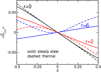
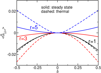
Figure 1: Comparison of the steady-state and thermal expectation values of $\tilde{G}_{j,j+r}$ as a function of the quench amplitude $\delta$ for $j=0$ and different even $r$. At fixed $r$ the two values agree to order $\delta$ (leading order thermalization). The more local the observable the longer the linear term prevails, that is the longer the steady-state and thermal values agree, when $|\delta|$ is increased.

Figure 2: The same as in Fig. 2 but for odd $r$. The leading $\delta$-dependence is of second order (‘factor of two class’ observables). For $r=1$ the prefactors of the second order terms agree and we find second order thermalization (‘thermalization class’ operator). This does not hold for $r=3,5$ as further analyzed in Fig. 3. The more local the observable the longer the steady-state and thermal values agree when $|\delta|$ is increased.

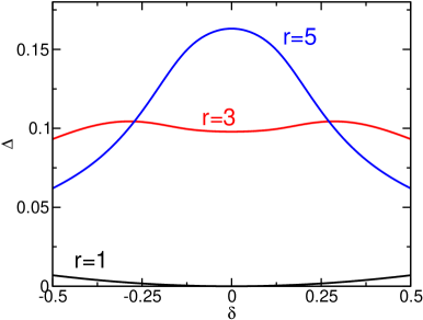
Figure 3: The difference $\Delta=\left|\left<\tilde{G}_{j,j+r}\right>_{\rm ss}-\left<\tilde{G}_{j,j+r}\right>_{\rm th}\right|/\delta^{2}$ as a function of $\delta$ for $j=0$ and different odd $r$. The vanishing of $\Delta$ for $\delta\to 0$ and $r=1$ shows that $\tilde{G}_{j,j+1}$ is a ‘thermalization class’ operator. For odd $r>1$, $\tilde{G}_{j,j+r}$ is not from this class but still from the ‘factor of two class’ (see Fig. 2).

We finally compare results for $\left<\tilde{G}_{j,j+r}\right>_{\rm ss}$ and $\left<\tilde{G}_{j,j+r}\right>_{\rm th}$ obtained by numerically solving the integrals in the exact expressions Eqs. (43) to (50). Figure 2 shows $\left<\tilde{G}_{j,j+r}\right>_{\rm ss/th}$ as a function of $\delta$ for $r=0,2,6$. Consistent with our analytical insights the steady-state and thermal expectation values agree to linear order (first order thermalization). We observe that the smaller $r$, that is the more local the observable, the longer the linear term prevails for increasing $|\delta|$. Figure 2 shows $\left<\tilde{G}_{j,j+r}\right>_{\rm ss/th}$ as a function of $\delta$ for $r=1,3,5$. The just described trend on the locality of the observable and the agreement of the steady-state and thermal expectation values obviously also holds for odd $r$. For such $r$, $\tilde{G}_{j,j+r}$ is a ‘factor of two class’ operator and the steady-state expectation value is ${\mathcal{O}}(\delta^{2})$. As just shown analytically, the same holds for $\left<\tilde{G}_{j,j+r}\right>_{\rm th}$. This is consistent with our numerical results. Being order $g^{2}$ the expectation values for small $|\delta|$ are rather small. To further investigate the second order term in Fig. 3 we show $\Delta=\left|\left<\tilde{G}_{j,j+r}\right>_{\rm ss}-\left<\tilde{G}_{j,j+r}\right>_{\rm th}\right|/\delta^{2}$ for the data of Fig. 2. For $r=1$, $\tilde{G}_{j,j+r}$ is a ‘thermalization class’ operator and $\lim_{\delta\to 0}\Delta=0$. In contrast, for $r=3,5$, $\tilde{G}_{j,j+r}$ is not from this class and $\lim_{\delta\to 0}\Delta$ remains finite; for odd $r>1$, $\tilde{G}_{j,j+r}$ does thus not thermalize to second order.

Our computations exemplify that for small even or odd $r$, that is a local $\tilde{G}_{j,j+r}$, and small $|\delta|$, either the differences or the absolute values of the expectation values are rather small. It indicates that based on purely numerical data obtained for models which cannot be solved exactly and which are prone to errors – for examples see Sect. V – it will be very difficult to make any definite statements on thermalization for small quenches.

IV Interaction quench in the Tomonaga-Luttinger model

In this section we study steady-state expectation values of a variety of observables after small interaction quenches in the spinless TL model.Giamarchi03 ; Schoenhammer05 The quench dynamics of the TL model was studied before,Cazalilla06 ; Uhrig09 ; Iucci09 ; Rentrop12 ; Karrasch12 however, not in the context of interest to us. This continuum model presents one of the rare examples in which closed analytical expressions for the expectation values of observables and correlation functions at all times can be obtained for an interacting system. To achieve this bosonization is used. This method consists of two steps. First the fermionic Hamiltonian is rewritten in terms of collective bosonic degrees of freedom (bosonization of the Hamiltonian). This is possible as right- and left-moving fermions with linear dispersion as well as two-particle scattering processes with only small momentum transfer are considered. To be able to compute all fermionic expectation values of interest, in a second step one has to express the fermionic field in terms of the bosons (bosonization of the field operator).Schoenhammer05 ; vonDelft98 We here adopt the notation and conventions of Ref. Rentrop12, .

IV.1 The Hamiltonian and eigenstates

The bosonized Hamiltonian is given by

$$H=\sum_{n>0} \left[k_{n}\left(v_{\rm F}+\frac{v(k_{n})}{2\pi}\right)\left(b_{n}^{\dagger}b_{n}+b_{-n}^{\dagger}b_{-n}\right)\right.$$

$$\left.+k_{n}\frac{v(k_{n})}{2\pi}\left(b_{n}^{\dagger}b_{-n}^{\dagger}+b_{-n}b_{n}\right)\right],$$ (57)

with bosonic operators $b_{n}^{({\dagger})}$, $n\in{\mathbb{Z}}$, which are linked to the densities $\rho_{n,\pm}$ of the right($+$)- and left($-$)-moving fermions in momentum space by

$$b_{n}=\frac{1}{\sqrt{|n|}}\left\{\begin{array}[]{cc}\rho_{n,+}&\mbox{for}\;n>0\\ \rho_{n,-}&\mbox{for}\;n<0\end{array}\right.,$$ (60)

and which obey the standard commutation relations. The two-particle potential is denoted as $v(k)$, the Fermi velocity as $v_{\rm F}$, and momenta are given by $k_{n}=n2\pi/L$ (periodic boundary conditions) with system size $L$. For vanishing interaction $v(k)=0$ the $b_{n}^{({\dagger})}$ are the eigenmode ladder operators and the boson dispersion is $\omega_{0}(k)=v_{\rm F}|k|$. We note that the interaction only couples the modes with fixed $|n|$. The Hamiltonian is thus a sum of commuting terms and the problem of finding the new eigenmodes factorizes. The eigenstates are product states (over $n\in{\mathbb{N}}$).

By a Bogoliubov transform $H$ can straightforwardly be diagonalized

$$H=\sum_{n\neq 0}\omega(k_{n})\,\alpha_{n}^{\dagger}\alpha_{n}+E_{\rm gs}$$ (61)

in terms of the eigenmodes

$$\alpha_{n}=c(k_{n})b_{n}-s(k_{n})b_{-n}^{\dagger}$$ (62)

with

$$s^{2}(k)=\frac{1}{2}\left[\frac{1+\hat{v}(k)/2}{\sqrt{1+\hat{v}(k)}}-1\right],\;c^{2}(k)=1+s^{2}(k),$$

$$\omega(k)=v_{\rm F}\,|k|\,\sqrt{1+\hat{v}(k)},$$ (63)

and the dimensionless potential $\hat{v}(k)=v(k)/(\pi v_{\rm F})$. For small interactions

$$s^{2}(k)=\hat{v}^{2}(k)/16+{\mathcal{O}}(\hat{v}^{3}).$$ (64)

We assume that the Fourier transform $v(q)$ of the two-particle potential is an even function which for $q>0$ decreases monotonically on a characteristic scale $q_{\rm c}$. It can be expressed as a function of $q/q_{\rm c}$. In integrals over momenta we often substitute $q^{\prime}=q/q_{\rm c}$ which implies $\hat{v}(q)=\hat{v}(q_{\rm c}q^{\prime})$, $c^{2}(q)=c^{2}(q_{\rm c}q^{\prime})$, …. We here focus on two-particle potentials with $\hat{v}(0)\geq 0$.

The nondegenerate ground state of $H$ is given by the product state (over the mode index) of the vacua with respect to the eigenmodes $\left|\mbox{vac}(\alpha)\right>$ and

$$E_{\rm gs}=-2\sum_{n>0}\omega(k_{n})\,s^{2}(k_{n})$$ (65)

is the ground-state energy. The excited states can be constructed by populating the bosonic states of the different eigenmodes $n$. Momentum conservation of the Hamiltonian Eq. (57) implies that every excited state is at least doubly degenerate. Depending on the momentum dependence of the eigenmode dispersion $\omega(k)$ Eq. (63) and thus the momentum dependence of the (dimensionless) two-particle potential $\hat{v}(k)$ further degeneracies might appear. Note that often $\omega(k)$ is linearized (in $k$) which leads to a vast number of degeneracies. However, all eigenstates are product states over the mode index $n\in{\mathbb{N}}$ and every factor is uniquely determined by the energy and the momentum contained in the given mode. Employing this one can generalize the proof of Sect. II.2 for time averages which is then based on an analog of Eq. (6) with the state being one of the factors of the many-body eigenstate. We refrain from going into details as even the direct applicability of the considerations of Sect. II.2 for the TL model does not imply that time-averaged and steady-state expectation values are equal (see the discussion of Sect. I.3).

To be able to compute arbitrary fermionic expectation values one has to bosonize the field operator. We here focus on the right-moving particles with momentum space ladder operators $c_{n,+}^{({\dagger})}$ and field operator

$$\psi_{+}^{\dagger}(x)=\frac{1}{\sqrt{L}}\sum_{n}e^{-ik_{n}x}c_{n,+}^{\dagger}\;\;.$$ (66)

One can prove the operator identity Schoenhammer05 ; vonDelft98

$$\psi^{\dagger}_{+}(x)=\frac{e^{-ix\pi/L}}{\sqrt{L}}e^{-i\Phi^{\dagger}(x)}U^{\dagger}e^{-i\Phi(x)}\;\;,$$ (67)

with

$$\Phi(x)=\frac{\pi}{L}Nx-i\sum_{n>0}e^{iq_{n}x}\left(\frac{2\pi}{Lq_{n}}\right)^{1/2}b_{n}\;\;,$$ (68)

where $N$ denotes the particle number operator and $U^{\dagger}$ a unitary fermionic raising operator which commutes with the $b_{n}^{({\dagger})}$. It maps the $N$-electron ground state to the $(N+1)$-electron one. Particle number contributions do not matter for our considerations and will not be discussed in detail. We emphasize that the relation between the original fermionic degrees of freedom and the bosonic eigenmodes is highly nonlinear.

As the initial state we consider the ground state of the noninteracting Hamiltonian Eq. (57) with $v(k)=0$. It corresponds to the product state of the vacua with respect to the $b_{n}$, $\left|E_{0}^{\rm i}\right>=\left|\mbox{vac}(b)\right>$, and the ground-state energy $E_{0}^{\rm i}$ vanishes. The excited states are constructed by filling the bosonic modes associated to the $b_{n}^{({\dagger})}$. The time evolution is performed with the two-particle interaction switched on and $H_{\rm f}$ given by Eq. (57). The (dimensionless) quench parameter is the amplitude of the two-particle potential $\hat{v}(0)$ at vanishing momentum transfer.

IV.2 The observables

As ‘observables’ we consider the kinetic energy

$$H_{0}=\sum_{n\neq 0}v_{\rm F}|k_{n}|b_{n}^{\dagger}b_{n}=H_{\rm i},$$ (69)

which is equivalent to the initial Hamiltonian, the operator content of the density-density correlation function of the right movers

$$D(x)=\rho_{+}(x)\rho_{+}(0)=\frac{1}{L^{2}}\sum_{n,n^{\prime}\neq 0}e^{ik_{n}x}\rho_{n,+}\rho_{n^{\prime},+},$$ (70)

as well as the one of the single-particle Green function of the right movers

$$G(x)=\psi_{+}^{\dagger}(x)\psi_{+}(0).$$ (71)

We note that for arbitrary $x$, $D(x)$ and $G(x)$ do not commute with $H_{\rm i}=H_{0}$ and do thus not fall into the class of operators considered in Refs. Moeckel08, and Moeckel09, .

We explicitely show that $\tilde{D}(x)$ and $\tilde{G}(x)$ are ‘factor of two class’ operators by computing their steady-state and interacting ground state expectation values.

Employing Eq. (60) $D(x)$ can be written as

$$D(x)=\frac{1}{2\pi L}\sum_{l,l^{\prime}>0} \sqrt{k_{l}k_{l^{\prime}}}\left(e^{ik_{l}x}b_{l}b_{l^{\prime}}+e^{ik_{l}x}b_{l}b_{l^{\prime}}^{\dagger}\right.$$

$$\left.+e^{-ik_{l}x}b_{l}^{\dagger}b_{l^{\prime}}+e^{-ik_{l}x}b_{l}^{\dagger}b_{l^{\prime}}^{\dagger}\right).$$ (72)

To show that Eq. (26) defining the ‘thermalization class’ holds for small $x$ we employ that $H_{\rm i}$ and $H_{\rm f}$ both conserve the total momentum $\sim\sum_{l\neq 0}k_{l}b_{l}^{\dagger}b_{l}$ and that $b_{l}^{({\dagger})}$ destroys (creates) a momentum $k_{l}$. Both ensures that in the steady-state and thermal expectation values of $D(x)$ Eq. (72) only the second and the third term with $l=l^{\prime}$ contribute. Furthermore, for $x=0$ the exponential terms in Eq. (72) are equal to 1 and $D(0)$ is proportional to the positive momentum part of the kinetic energy $H_{\rm i}$. In the steady-state and thermal expectation values of the kinetic energy the positive and negative momentum parts of the sum contribute equally (by symmetry). Up to the prefactor $(2\pi v_{\rm F}L)^{-1}$, these expectation values of $D(0)$ are thus equal to the ones of $H_{0}$. Thus the local operator $\tilde{D}(0)$ is element of the ‘thermalization class’. Comparing the steady-state and thermal expectation values of $D(0)$ we explicitely verify that it thermalizes to second order in the two-particle interaction.

Employing Eqs. (66) to (68) and the Baker-Campbell-Hausdorff formula $G(x)$ can be written as

$$G(x)=G_{0}(x) \exp\left\{\sum_{l>0}\frac{e^{-ik_{l}x}-1}{\sqrt{l}}b_{l}^{\dagger}\right\}$$

$$\times\exp\left\{\sum_{l^{\prime}>0}\frac{1-e^{ik_{l^{\prime}}x}}{\sqrt{l^{\prime}}}b_{l^{\prime}}\right\},$$ (73)

with

$$G_{0}(x)=\frac{1}{L}\,\frac{e^{-ik_{\rm F}x}}{1-e^{i(2\pi x/L+i0)}}.$$ (74)

Following the same reasoning as for $D(0)$ it is straight forward to show that

$$\frac{\left<G(x)\right>_{\rm ss/th}}{G_{0}(x)}=1-x^{2}\frac{2\pi}{L}\sum_{l>0}k_{l}\left<b_{l}^{\dagger}b_{l}\right>_{\rm ss/th}+{\mathcal{O}}(x^{4}).$$ (75)

This shows that for small $x$, $G(x)$ is from the ‘thermalization class’. Comparing the steady-state and thermal expectation values of $G(x)$ at small $x$ we explicitely verify that it thermalizes to second order.

observable	first order therm.	fact 2 cl.	therm. cl.
$\tilde{G}(x)$	first order vanishes	yes	for $q_{\rm c}x\ll 1$
$\tilde{D}(x)$	first order vanishes	yes	for $q_{\rm c}x\ll 1$
$\tilde{H}_{\rm i}$	first order vanishes	yes	yes
$\rho(x)$	yes	no	no

Table 2: Classification of the considered operators.

We furthermore verify that Eq. (24) holds for

$$V=\sum_{n>0} \left[k_{n}\frac{v(k_{n})}{2\pi\hat{v}(0)}\left(b_{n}^{\dagger}b_{n}+b_{-n}^{\dagger}b_{-n}\right)\right.$$

$$\left.+k_{n}\frac{v(k_{n})}{2\pi\hat{v}(0)}\left(b_{n}^{\dagger}b_{-n}^{\dagger}+b_{-n}b_{n}\right)\right]$$ (76)

[see Eq. (4)]. With the results of Sect. II.5 we can thus be sure that all ‘thermalization class’ operators thermalize to second order in $\hat{v}(0)$.

The classification of the considered operators is summarized in Table 2.

IV.3 The time evolution and steady state

Employing Eq. (67), the simple time dependence of the eigenmode ladder operators

$$\alpha_{n}(t)=e^{-i\omega(k_{n})t}\,\alpha_{n},\quad\alpha_{n}^{{\dagger}}(t)=e^{i\omega(k_{n})t}\,\alpha_{n}^{{\dagger}},$$ (77)

the ladder operator properties of the $b_{n}^{({\dagger})}$ and $\alpha_{n}^{({\dagger})}$, as well as the knowledge of the interacting and noninteracting ground states the time evolution of the expectation values of our observables out of the noninteracting ground state can be computed straightforwardly. After the thermodynamic limit was taken – note that the kinetic energy is extensive and must first be divided by $L$ – the limit $t\to\infty$ can be performed and the expectation values assume steady-state values.

For the dimensionless kinetic energy per length we obtain

$$e_{\rm ss}=\lim_{L\to\infty}\frac{\left<\tilde{H}_{0}\right>_{\rm ss}}{v_{\rm F}q_{\rm c}^{2}L}=\frac{2}{\pi}\int_{0}^{\infty}dqqs^{2}(q_{\rm c}q)c^{2}(q_{\rm c}q),$$ (78)

where we have substituted $q/q_{\rm c}\to q$.

The dimensionless steady-state expectation value of $\tilde{D}(x)$ is given by

$$q_{\rm c}^{-2}\left<\tilde{D}(x)\right>_{\rm ss}=\frac{1}{\pi^{2}}\int_{0}^{\infty}dqqs^{2}(q_{\rm c}q)c^{2}(q_{\rm c}q)\cos[q(q_{\rm c}x)].$$ (79)

If we expand the cosine function on the right-hand side for small $q_{\rm c}|x|$ and keep only the leading term we obtain

$$q_{\rm c}^{-2}\left<\tilde{D}(x)\right>_{\rm ss}= \frac{1}{\pi^{2}}\int_{0}^{\infty}dqqs^{2}(q_{\rm c}q)c^{2}(q_{\rm c}q)+{\mathcal{O}}([q_{\rm c}x]^{2})$$

$$= \frac{1}{2\pi}e_{\rm ss}+{\mathcal{O}}([q_{\rm c}x]^{2}).$$ (80)

In the last step we used Eq. (78). The relation between the local part of the steady-state expectation value of $\tilde{D}(x)$ and the kinetic energy is in accordance with the discussion following Eq. (72).

We finally consider the single-particle Green function $G(x)$. Its steady state expression was derived earlier; see e.g. Eq. (33) of Ref. Rentrop12, . It can be written as

$$\left<\tilde{G}(x)\right>_{\rm ss}=G_{0}(x)\left[e^{g_{\rm ss}(x)}-1\right],$$ (81)

with

$$g_{\rm ss}(x)=4\int_{0}^{\infty}dqs^{2}(q_{\rm c}q)c^{2}(q_{\rm c}q)\frac{\cos[q(q_{\rm c}x)]-1}{q}.$$ (82)

For $q_{\rm c}|x|\ll 1$, $g_{\rm ss}(x)$ further simplifies to

$$g_{\rm ss}(x) =-2(q_{\rm c}x)^{2}\int_{0}^{\infty}dqqs^{2}(q_{\rm c}q)c^{2}(q_{\rm c}q)+{\mathcal{O}}([q_{\rm c}x]^{4})$$

$$=-\pi(q_{\rm c}x)^{2}e_{\rm ss}+{\mathcal{O}}([q_{\rm c}x]^{4})$$ (83)

[for the second line see Eq. (78)] and thus

$$\frac{\left<\tilde{G}(x)\right>_{\rm ss}}{G_{0}(x)}=-\pi(q_{\rm c}x)^{2}e_{\rm ss}+{\mathcal{O}}([q_{\rm c}x]^{4}),$$ (84)

in accordance with Eq. (75).

The steady-state expectation values can also be obtained using a GGE.Cazalilla06 As for the quench in the tight-binding chain we, however, preferred to compute the full time evolution to verify that all the observables of interest become stationary.

IV.4 The thermal expectation values

We next compute the thermal expectation values.

The effective temperature corresponding to the energy quenched into the system is determined by

$$\lim_{L\to\infty}\frac{\left<\mbox{vac}(b)\right|H_{\rm f}\left|\mbox{vac}(b)\right>}{L}\overset{!}{=}\lim_{L\to\infty}\frac{1}{LZ_{\rm f}}\mbox{Tr}\left(e^{-H_{\rm f}/T_{\rm f}}H_{\rm f}\right)$$

$$\Leftrightarrow 0\overset{!}{=}\int_{0}^{\infty}dk\omega(k)\left[n\left(\frac{\omega(k)}{T_{\rm f}}\right)-s^{2}(k)\right],$$ (85)

where $n(x)=\left[e^{x}-1\right]^{-1}$ is the Bose function. We note that for the phonon-like bosons $\alpha_{n}^{({\dagger})}$ the chemical potential vanishes. Equation (85) can straightforwardly be solved numerically. For small quenches $|\hat{v}(0)|\ll 1$ we can make analytical progress using Eq. (64) and obtain

$$\left(\frac{T_{\rm f}}{v_{\rm F}q_{\rm c}}\right)^{2}=\frac{3}{8\pi^{2}}\int_{0}^{\infty}dqq\hat{v}^{2}(q_{\rm c}q)+{\mathcal{O}}\left(\hat{v}^{3}(0)\right).$$ (86)

This is consistent with Eq. (20).

The thermal expectation values of our observables can be computed employing the same ideas as used for the time evolution. They are given by

$$e_{\rm th}= \frac{1}{\pi}\int_{0}^{\infty}dqq$$

$$\times\left[s^{2}(q_{\rm c}q)+\left\{1+2s^{2}(q_{\rm c}q)\right\}n\left(\frac{\omega(q_{\rm c}q)}{T_{\rm f}}\right)\right]$$ (87)

for the kinetic energy,

$$q_{\rm c}^{-2} \left<\tilde{D}(x)\right>_{\rm th}=\frac{1}{2\pi^{2}}\int_{0}^{\infty}dqq\cos[q(q_{\rm c}x)]$$

$$\times\left[s^{2}(q_{\rm c}q)+\left\{1+2s^{2}(q_{\rm c}q)\right\}n\left(\frac{\omega(q_{\rm c}q)}{T_{\rm f}}\right)\right].$$ (88)

for the density-density-correlation function, and

$$\left<\tilde{G}(x)\right>_{\rm th}=G_{0}(x)\left[e^{g_{\rm th}(x)}-1\right],$$ (89)

with

$$g_{\rm th}(x) =2\int_{0}^{\infty}dq\frac{\cos[q(q_{\rm c}x)]-1}{q}$$

$$\times\left[s^{2}(q_{\rm c}q)+\left\{1+2s^{2}(q_{\rm c}q)\right\}n\left(\frac{\omega(q_{\rm c}q)}{T_{\rm f}}\right)\right]$$ (90)

for the single-particle Green function. Remarkably, in all expressions the interaction and temperature enter via the same factor given by the square brackets.

IV.5 Comparison

We are now in a position to explicitly confirm Eq. (7) (with $\overline{\left<\ldots\right>}$ replaced by $\left<\ldots\right>_{\rm ss}$) for all the considered observables. Expanding the steady-state expectation values Eqs. (78), (79), and (81) [with Eq. (82) inserted] for $|\hat{v}(0)|\ll 1$ leads to

$$e_{\rm ss}=\frac{1}{8\pi}\int_{0}^{\infty}dqq\hat{v}^{2}(q_{\rm c}q)+{\mathcal{O}}\left(\hat{v}^{3}(0)\right),$$ (91)

$$q_{\rm c}^{-2}\left<\tilde{D}(x)\right>_{\rm ss}= \frac{1}{16\pi^{2}}\int_{0}^{\infty}dqq\hat{v}^{2}(q_{\rm c}q)\cos[q(q_{\rm c}x)]$$

$$+{\mathcal{O}}\left(\hat{v}^{3}(0)\right),$$ (92)

and

$$\frac{\left<\tilde{G}(x)\right>_{\rm ss}}{G_{0}(x)}= \frac{1}{4}\int_{0}^{\infty}dq\hat{v}^{2}(q_{\rm c}q)\frac{\cos[q(q_{\rm c}x)]-1}{q}$$

$$+{\mathcal{O}}\left(\hat{v}^{3}(0)\right),$$ (93)

where we used Eq. (64). Setting $T_{\rm f}=0$ and thus $n(\omega(q_{\rm c}q)/T_{\rm f})\to 0$ in Eqs. (87), (88), and (90) we obtain the ground-state expectation values of our observables with respect to $H_{\rm f}$. If we expand the resulting expressions for $|\hat{v}(0)|\ll 1$ employing Eq. (64) we recover Eqs. (91), (92), and (93) up to a factor $1/2$ which confirms Eq. (7); all the considered observables are from the ‘factor of two class’.

We next explicitly investigate thermalization to order $\hat{v}^{2}(0)$. We start out with the thermal kinetic energy Eq. (87). For $T_{\rm f}>0$ also the second term in the square brackets associated to thermal excitations contributes. For small quenches we can use that $T_{\rm f}$ is of order $\hat{v}(0)$ [see Eq. (86)] and obtain

$$e_{\rm th}= \frac{1}{\pi}\int_{0}^{\infty}dqq\Big{[}\underbrace{\frac{1}{16}\hat{v}^{2}(q)}_{T_{\rm f}=0-\mbox{\scriptsize contr.}}+\underbrace{n\left(\frac{\omega_{0}(q_{\rm c}q)}{T_{\rm f}}\right)}_{T_{\rm f}>0-\mbox{\scriptsize contr.}}\Big{]}+{\mathcal{O}}\left(\hat{v}^{3}(0)\right)$$

$$= \frac{1}{\pi}\int_{0}^{\infty}\!\!\!\!\!dq\Big{[}\underbrace{\frac{q}{16}\hat{v}^{2}(q)}_{T_{\rm f}=0-\mbox{\scriptsize contr.}}+\underbrace{\left(\frac{T_{\rm f}}{v_{\rm F}q_{\rm c}}\right)^{2}\frac{q}{e^{q}-1}}_{T_{\rm f}>0-\mbox{\scriptsize contr.}}\Big{]}+{\mathcal{O}}\left(\hat{v}^{3}(0)\right)$$

$$= \frac{1}{\pi}\int_{0}^{\infty}\!\!\!\!\!dq\Big{[}\underbrace{\frac{q}{16}\hat{v}^{2}(q)}_{T_{\rm f}=0-\mbox{\scriptsize contr.}}+\underbrace{\frac{q}{16}\hat{v}^{2}(q)}_{T_{\rm f}>0-\mbox{\scriptsize contr.}}\Big{]}+{\mathcal{O}}\left(\hat{v}^{3}(0)\right).$$ (94)

In the last step we used Eq. (86) and $\int_{0}^{\infty}dqq/(e^{q}-1)=\pi^{2}/6$. The ground-state contribution and the one from the thermal excitations at $T_{\rm f}$ – both being equal – add up to give the steady-state expectation value Eq. (91) up to corrections of order $\hat{v}^{3}(0)$. This confirms thermalization to quadratic order and provides yet another example for our explanation of the factor of 2 in Eq. (7) for observables which are simultaneously from the ‘factor of two class’ and the ‘thermalization class’.

After expanding the cosine appearing in Eqs. (88) and (90) to lowest nonvanishing order the same steps can be performed as the remaining integrals are exactly of the form which appeared in the analysis of the kinetic energy. Thus $D(x)$ thermalizes to order $\hat{v}^{2}(0)$ up to corrections of order $(q_{\rm c}x)^{2}$ and $G(x)$ up to corrections of order $(q_{\rm c}x)^{4}$. In other words, the local parts of $D(x)$ and $G(x)$ thermalize for small quenches. The factor of two of Eq. (7) can again be traced back to the two equal contributions from the ground state and the thermal excitations.

This is in full agreement with the general results of Sect. II.5. The operator content of the first term of $V$ Eq. (76) is identical to that of the kinetic energy. For the latter we have just shown that the steady-state and thermal expectation values are identical up to corrections of order $\hat{v}^{3}(0)$. Thus the same holds for this contribution to $V$. To show that also the second term in $V$ fulfills Eq. (24) does also not require any additional computations. When computing thermal expectation values of products of two $b$ ladder operators temperature always enters via the Bose function. As we have just seen when going from the first to the second line in Eq. (94) $q$ times the Bose function always contributes a factor $T_{\rm f}^{2}\sim\hat{v}^{2}(0)$. The $T_{\rm f}=0$ and $T_{\rm f}>0$ expectation values thus agree up to corrections of order $\hat{v}^{2}(0)$ and Eq. (24) holds for $V$ of Eq. (76).

IV.6 The density in the semi-infinite Tomonaga-Luttinger model

The observables we considered so far for the TL model were all from the ‘factor of two class’ and, if local, in addition from the ‘thermalization class’. To provide an example of an observable which does not fall into the ‘factor of two class’, we investigate the density $\rho_{+}(x)=\psi_{+}^{\dagger}(x)\psi_{+}(x)$. For a translationally invariant system its expectation value is $x$-independent and turns out to be time-independent after the interaction quench. Neither is true if we consider the TL model with open boundary conditions.Fabrizio95 The quench dynamics of the TL model in the presence of open boundaries was studied earlier.Kennes13 The exact computation of the quench dynamics of this model requires so-called open boundary bosonization.Fabrizio95 ; Meden00 ; Grap09 We here refrain from giving details and only report on the results. The steps required to obtain these are very similar to the ones taken above for the quench dynamics of the translationally invariant TL model.

In the long-time limit the density becomes stationary and its steady-state expectation value $d_{\rm ss}(x)$ is given by

$$\frac{d_{\rm ss}(x)}{d_{0}(x)}=\exp\Biggl{\{} \int_{0}^{\infty}dq2s(q_{\rm c}q)c(q_{\rm c}q)\left[s(q_{\rm c}q)+c(q_{\rm c}q)\right]^{2}$$

$$\times\frac{\cos[q(q_{\rm c}x)]-1}{q}\Biggr{\}},$$ (95)

where $d_{0}(x)$ denotes the density of the open system at vanishing two-particle interaction. The thermal expectation value is

$$\frac{d_{\rm th}(x)}{d_{0}(x)}=\exp\Biggl{\{}\int_{0}^{\infty}dq2 \Biggl{[}s^{2}(q_{\rm c}q)+s(q_{\rm c}q)c(q_{\rm c}q)$$

$$+\left\{s(q_{\rm c}q)+c(q_{\rm c}q)\right\}^{2}n\left(\frac{\omega(q_{\rm c}q)}{T_{\rm f}}\right)\Biggr{]}$$

$$\times\frac{\cos[q(q_{\rm c}x)]-1}{q}\Biggr{\}}.$$ (96)

Via the term $s(q_{\rm c}q)c(q_{\rm c}q)$ the interaction now enters to linear order in $\hat{v}(0)$; $\rho_{+}(x)$ of the semi-infinite TL model is not from the ‘factor of two class’. To order $\hat{v}(0)$ the argument of the exponential function in $d_{\rm ss}(x)$ and $d_{\rm th}(x)$ is equal to $-\hat{v}(q_{\rm c}q)\{\cos[q(q_{\rm c}x)]-1\}/(2q)$ and the density thermalizes to order $\hat{v}(0)$. We emphasize that this holds independently of the position $x$ away from the open boundary; there is no requirement of locality for first order thermalization. Furthermore, to leading order $T_{\rm f}$ in Eq. (96) can be set to zero and Eq. (5) with $\overline{\left<\ldots\right>}$ replaced by $\left<\ldots\right>_{\rm ss}$ holds.

V Interaction quenches for spinless lattice fermions

V.1 The Hamiltonians and DMRG

Finally, we study interacting spinless fermions on a lattice of size $M$ described by the Hamiltonian

$$H= -\frac{1}{2}\sum_{j=1}^{M}\left(c_{j+1}^{\dagger}c_{j}+\mbox{H.c.}\right)$$

$$+U\sum_{j=1}^{M}\left(n_{j}-\frac{1}{2}\right)\left(n_{j+1}-\frac{1}{2}\right),$$ (97)

where $n_{j}=c_{j}^{\dagger}c_{j}$ is the density. The nearest-neighbor density-density-type two-particle interaction has the (dimensionless) strength $U$. We focus on repulsive interactions $U>0$ and half-filling of the band. Note that in contrast to the Hamiltonian of Sect. III where the amplitude of the nearest-neighbor hopping $J$ was set to $1$ it will turn out to be more convenient to take $J=1/2$ here. With this choice the bandwidth is two. The model can be mapped onto the XXZ-Heisenberg spin chain

$$H=\sum_{j=1}^{M}\left(S^{x}_{j+1}S^{x}_{j}+S^{y}_{j}S^{y}_{j+1}\right)+U\sum_{j=1}^{M}S^{z}_{j}S^{z}_{j+1},$$ (98)

using a Jordan-Wigner transform. The $S_{j}^{\zeta}$, with $\zeta=x,y,z$, denote spin-1/2 operators. This simple form justifies a posteriori the choice $J=1/2$. The spin Hamiltonian is convenient when using DMRG.

The XXZ-Heisenberg spin chain is Bethe ansatz solvable. Therefore, many of its equilibrium properties are known analytically (see e.g. Refs. Giamarchi03, and Schoenhammer05, ). The system is gapless for $0\leq U<1$, while for $U>1$ a gap opens. In the latter regime long-ranged anti-ferromagnetic ordering emerges – charge-density-wave order in the language of the fermions. The former displays (metallic) Luttinger liquid behavior. The model is characterized by an extensive set of (quasi-) local integrals of motion and thus constitutes a prototypical model of the class (iii) defined in the Introduction.

The implications of this set of conserved quantities on the relaxation dynamics was heavily debated.Gogolin15 We stress that our general considerations of Sect. II do not make use of integrals of motion and our predictions are thus valid in the presence as well as in the absence of such a set. To emphasize this we in addition study a model in which the nearest-neighbor interaction is supplemented by a next-nearest-neighbor one with (dimensionless) strength $W\geq 0$

$$H= \sum_{j=1}^{M}\left(S^{x}_{j+1}S^{x}_{j}+S^{y}_{j}S^{y}_{j+1}\right)+U\sum_{j=1}^{M}S^{z}_{j}S^{z}_{j+1}$$

$$+W\sum_{j=1}^{M}S^{z}_{j}S^{z}_{j+2}.$$ (99)

For such a system a Bethe ansatz solution is not known. It is generally believed that the model is not solvable employing this method. The model thus represents the most generic class (iv). The equilibrium phase diagram including the next-nearest-neighbor interaction is more complicated, but displays an extended gapless phase at small $U$ and small $W$.

Besides the degeneracies associated to translation invariance at least for $U=W=0$ further ‘accidental’ degeneracies can be found.Deguchi01 ; Fagotti14a The same considerations as in Sect. III hold and Eq. (6) cannot be exploited directly.

As the initial state we consider the nondegenerate ground state $\left|E^{\rm i}_{0}\right>$ for $U=W=0$ (odd number of particles) and perform the time evolution with respect to finite $U$ and possibly $W$. Thus for small quenches the system will remain in its gapless phase, which is at the center of our interest. For completeness we will also show results for gapped systems (after the quench) to illustrate how the perturbatively motivated analytical insights become invalid at larger interactions.

As the Hamiltonians introduced above include two-particle interactions which are difficult to treat analytically, we rely on the numerically exact DMRG in the following. The accuracy of the DMRG is (in practice) controlled by a numerical parameter called the bond dimension $\chi$. Increasing $\chi$ and with it the numerical effort, one can achieve converged results. In the following $\chi$ is always chosen such that no changes of the results can be observed on the scales of the respective plots if it is further increased (‘numerically exact results’).

We are left with performing three tasks: (a) preparing the ground state of the noninteracting ($U=0=W$) system, (ii) subsequently performing the time evolution with respect to finite $U$ and possibly $W$ and (iii) calculating the finite temperature canonical ensemble with respect to finite $U$ and possibly $W$ (which is independent of the previous two tasks).

We implement our DMRG algorithm using the language of matrix product states (MPS) and so-called infinite boundary conditions, which can be coded very elegantly. More importantly, one obtains results directly in the thermodynamic limit $M\to\infty$Vidal07 ; Orus08 and does not need to perform a finite-size scaling analysis.Karrasch12a As the algorithms are well documentedSchollwoeck11 we will skip the technical details and provide only an overview. The ground state is found via an iterative procedure. One starts with a random MPS and repetitively applies $e^{-H_{\rm i}\Delta\tau}$, normalizing the MPS after each step. To apply $e^{-H_{\rm i}\Delta\tau}$ we choose a second order Trotter decomposition. We start with larger values of $\Delta\tau$ and successively lower it until the MPS converges to $\left|E^{\rm i}_{0}\right>$. We aim at a relative accuracy of the total energy per lattice site of $10^{-10}$; after this is reached we stop the algorithm. It is straightforward to benchmark the outcome of this procedure, as the ground state preparation is done for the noninteracting system $U=0=W$. Next we perform a real-time evolution of this MPS by repetitively applying $e^{-iH_{\rm f}\Delta t}$, where we use a fourth order Suzuki-Trotter decomposition and choose $\Delta t$ small enough such that the error arising from this decomposition is negligible. To determine the finite temperature canonical ensemble we use purification at $\beta=1/T=0$ effectively rewriting the ensemble as an MPS in enlarged physical space.Verstraete04 Afterwards one can ‘cool down’ the MPS by repetitively applying $e^{-H_{\rm f}\Delta\beta}$ (and normalizing) in an appropriately Trotter decomposed fashion.

V.2 The observables

As in Sects. III and IV we consider several observables. We study the spin-spin correlations of the $z$-direction

$$C^{zz}_{r}=S^{z}_{j}S^{z}_{j+r},$$ (100)

which due to translation invariance are $j$-independent. As explicitly discussed below (see Figs. 4 and 5) $\left<E_{0}^{\rm i}\right|C^{zz}_{r}(t)\left|E_{0}^{\rm i}\right>$ converges towards a steady-state value for all $r$ and all parameter sets studied. The expectation values $\left\langle C^{zz}_{r}\right\rangle_{\rm ss/th}$ turn out to have a leading linear order dependence on the quench amplitude and $C^{zz}_{r}$ is neither from the ‘factor of two class’ nor the ‘thermalization class’. As shown in the lower panels of Figs. 6 (lower three) and 8 (lower two) the numerical results for the steady-state and ground state (with respect to $H_{\rm f}$) expectation values at sufficiently small $U$ are fully consistent with Eq. (5) where $\overline{\left<\ldots\right>}$ is replaced by $\left<\ldots\right>_{\rm ss}$ (compare the crosses and the solid lines). We thus expect Eq. (22) to hold for $\left\langle C^{zz}_{r}\right\rangle_{\rm ss/th}$ indicating thermalization to linear order.

We furthermore compute the kinetic energy per lattice site

$$\tilde{h}_{\rm kin}=\frac{1}{M}\left(H_{\rm{i}}-\left\langle E_{0}^{\rm i}\right|H_{\rm{i}}\left|E_{0}^{\rm i}\right\rangle\right),$$ (101)

where we have subtracted the value of the kinetic energy before the quench to eliminate an irrelevant constant. It takes a steady-state value; see Figs. 4 and 5. The numerical results for the steady-state expectation value of the kinetic energy are consistent with an order $g^{2}$ dependence; see the crosses in the upper panel of Figs. 6 and 8. A comparison of the crosses with the solid lines which show twice the ground state (with respect to $H_{\rm f}$) expectation values indicate that Eq. (7) with $\overline{\left<\ldots\right>}$ replaced by $\left<\ldots\right>_{\rm ss}$ holds; the kinetic energy is a ‘factor of two class’ operator. It is per definition from the ‘thermalization class’ and we expect thermalization to second order.

observable	first order therm.	fact 2 cl.	therm. cl.
$C^{zz}_{r}$	yes	no	no
$\tilde{h}_{\rm kin}$	first order vanishes	yes	yes
$\tilde{B}_{r}$	first order vanishes	yes	for $r=1$

Table 3: Classification of the considered operators.

Finally, we introduce observables which are of the ‘factor of two class’, but not necessarily of the ‘thermalization class’. A simple example of such are the fermionic bond operators

$$\tilde{B}_{r}=c_{j}^{\dagger}c_{j+r}+{\rm H.c.}-\left\langle E_{0}^{\rm i}\right|c_{j}^{\dagger}c_{j+r}+{\rm H.c.}\left|E_{0}^{\rm i}\right\rangle,$$ (102)

which take steady-state values (not shown). The system remains translationally invariant by one lattice site even after the quench. The expectation values (during the time evolution, in the steady state as well as in the thermal state) of the operator will thus be independent of $j$. This explains why we suppressed the index $j$ in the definition of $\tilde{B}_{r}$. The sum of $\tilde{B}_{r}$ over $j$ can be expressed in terms of the noninteracting eigenmode number operators $c_{k}^{\dagger}c_{k}$. Those in turn commute with $H_{\rm i}$ and the condition (c) of Refs. Moeckel08, and Moeckel09, to prove Eq. (2) is fulfilled; our generalization is not required. The combination of translational and particle-hole symmetry (at half-filling) ensures that $\left\langle\tilde{B}_{r}\right\rangle_{\rm ss}=0=\left\langle\tilde{B}_{r}\right\rangle_{\rm th}$ for even $r$. Thus we focus on $r$ being odd. As exemplified in Fig. 7 all $\tilde{B}_{r}$ are element of the ‘factor of two class’ (compare the crosses and solid lines). However, only $\tilde{B}_{1}$ can be related to the kinetic energy due to spatial translation invariance and is thus also of the ‘thermalization class’. Thus Eq. (7) with $\overline{\left<\ldots\right>}$ replaced by $\left<\ldots\right>_{\rm ss}$ holds for all $\tilde{B}_{r}$ but thermalization to second order can only be expected for $\tilde{B}_{1}$.

The classification of the considered operators is summarized in Table 3.

V.3 Time evolution towards the steady state

First, we benchmark the time scales accessible within our numerical DMRG approach at given computational resources and show that on these all observables of interest take steady-state values. To reach a designated accuracy in DMRG simulations the bond dimension $\chi$ must be increased for increasing entanglement of the system. As entanglement generically grows with time one can only reach a finite time scale (for given numerical resources).

We show the dynamics resulting out of different quench protocols in Figs. 4 and 5 for two different small quench amplitudes. The time evolution of the observables shows an initial transient behavior on times of the order of the inverse bandwidth. Within this transient regime the observables exhibit damped oscillatory behavior, where the amplitude almost perfectly dies out (on the scale of the plots) after times of the order of ten times the inverse bandwidth. Generically, the lower the value of $U$ and $W$ the larger is the time scale which can be reached at given resources (compare Figs. 4 and 5). This is very reasonable as larger quenches result in a larger entropy production and thus a larger entanglement growth. In any case one can access time scales of the order of a $100$ or $10$ times the inverse bandwidth for smaller and larger quenches, respectively. This is sufficient to extract what appears to be the steady value to high precision for all our observables and all parameter sets considered. This demonstrates the usefulness of the DMRG for the analysis we have in mind. Note that there is no notable difference in the time evolution for the cases of vanishing and finite $W$, that is for systems with an extensive set of (quasi-) local integrals of motion and without this. We emphasize, that we studied the time evolution for many more parameter sets and always found a behavior similar to the one shown in Figs. 4 and 5.

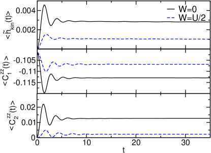
Figure 4: Time evolution of $\left<O(t)\right>=\left<E_{0}^{\rm i}\right|O(t)\left|E_{0}^{\rm i}\right>$ for different observables $O$ after an interaction quench with amplitude $U=0.25$, $W=0$ and $U=0.25$, $W=0.125$ obtained by DMRG. The initial state is the noninteracting ground state. For all observables the results become stationary for the times reachable.

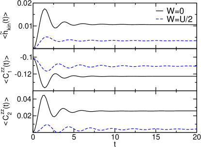
Figure 5: The same as in Fig. 4 but for $U=0.5$, $W=0$ and $U=0.5$, $W=0.25$. The larger the interaction quench the stronger the entanglement grows with time and the shorter the time scales reachable for given computational resources (compare to Fig. 4).

In the following, the steady state value of an observable is approximated by its value at the largest time reached within our simulation. Obviously purely based on the numerics we cannot rule out that at much larger time scales another relaxation mechanism sets in leading towards a different steady-state value. However, we cannot observe an indication of this in any of our data sets (for $W=0$ and $W>0$). In fact, the agreement of the steady-state value read off from the numerical data with the thermal expectation value according to our general considerations of Sects. II.4 and II.5 we discuss next gives us confidence that we have reached the ultimate steady state value. We emphasize that the observed single step relaxation of local observables is in accordance with the prethermalization conjecture.Berges04

V.4 Steady state for the model with nearest-neighbor interaction

We next compare the steady-state expectation value of our observables obtained after an interaction quench to their thermal counterparts. The temperature $T_{\rm f}$ of the thermal ensemble is computed using DMRG and Eq. (8) by an iterative procedure. The inset of Fig. 6 shows the effective temperature determined this way in dependence of $U$ after the quench in comparison to our order $U$ prediction Eq. (20).

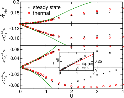
Figure 6: Comparison of the steady-state (crosses) and thermal (circles) expectation value for different observables as a function of the quench amplitude $U$. The kinetic energy (upper panel) is a ‘factor of two class’ as well as a ‘thermalization class’ operator. Accordingly its leading term is ${\mathcal{O}}(U^{2})$ with agreeing prefactors of the steady-state and thermal values. The solid line shows twice the ground state (with respect to $H_{\rm f}$) expectation value [see Eq. (7) with with $\overline{\left<\ldots\right>}$ replaced by $\left<\ldots\right>_{\rm ss}$]. The spin-spin correlations (lower three panels) are neither from the ‘factor of two class’ nor the ‘thermalization class’ and show thermalization to order $U$. The more local the observable, that is, the smaller $r$, the longer the linear order term prevails. The solid lines show the ground state (with respect to $H_{\rm f}$) expectation values [see Eq. (5) with with $\overline{\left<\ldots\right>}$ replaced by $\left<\ldots\right>_{\rm ss}$]. The inset shows the $U$-dependence of the effective temperature $T_{\rm f}$ (over the entire gapless phase) obtained numerically as well as from the order $U$ expression Eq. (20).

First, we focus on $W=0$ [model class (iii)] and consider the kinetic energy $\tilde{h}_{\rm kin}$ as well as the spin-spin correlations $C_{r}^{zz}$ with $r\in\{1,2,3\}$ as typical examples of local observables. As argued above, the kinetic energy is of the ‘factor of two class’ (compare crosses and line in the upper panel of Fig. 6) and by definition from the ‘thermalization class’, while the spin-spin correlator is neither element of the former nor the latter. The comparison is summarized in the main panels of Fig. 6, where the $x$-axis labeled by $U$ denotes the strength of the interaction after the quench. The steady-state and thermal kinetic energy show a leading $U^{2}$-dependence and within the accuracy of our numerics the two prefactors agree. This second order thermalization is in full agreement with our general considerations. This can be understood in more detail considering the spin-spin correlations. The steady-state as well as thermal expectation values of the three $r$ shown display a linear $U$-dependence. Within the accuracy of the results the prefactors of the steady-state and thermal values agree; the $C_{r}^{zz}$ thermalize to linear order in accordance with Sect. II.4. For the Hamiltonian (98) $C_{1}^{zz}$ is directly linked to $V$ of Eq. (4). Thus Eq. (24) holds and thermalization of $\tilde{h}_{\rm kin}$ to second order can be concluded from our considerations of Sect. II.5.

The numerical findings for the XXZ-chain are thus in full agreement with our ‘small-quench thermalization phenomenology’. A more sophisticated analysis to extract and compare the differences in the next to leading order (as performed in Sect. III) is currently beyond the accuracy of the DMRG results, as very small but finite contributions from the transient dynamics spoil this extremely sensitive numerical test.

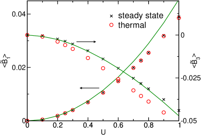
Figure 7: The same as in Fig. 6 but for the ‘factor of two class’ operators $\tilde{B}_{r}$ with odd $r$ (the expectation values for even $r$ vanish by symmetry). The solid line shows twice the ground state (with respect to $H_{\rm f}$) expectation value [see Eq. (7) with with $\overline{\left<\ldots\right>}$ replaced by $\left<\ldots\right>_{\rm ss}$]. The operator $\tilde{B}_{1}$ is directly related to the kinetic energy and thus in addition from the ‘thermalization class’. The prefactor of the leading $U^{2}$-terms of the steady-state and thermal expectation values agree (crosses and circles coincide for sufficiently small $U$). This does not hold for $\tilde{B}_{3}$.

In Fig. 6 we consider $U$ being as large as $4$, which means that the quench leads out of the gapless into the gapped phase of the system. We do so to illustrate how deviations of the thermal and steady state expectation values continuously develop at larger values of $U$. Surprisingly, the quantitative agreement between steady state and thermal expectation values of the local observables $\tilde{h}_{\rm kin}(t)$ and $C_{r}^{zz}$ with $r\in\{1,2\}$ is very good over a rather large range of $U$. The differences in the prefactors of the higher order terms – $\mathcal{O}(U^{3})$ and $\mathcal{O}(U^{2})$ for $\tilde{h}_{\rm kin}(t)$ and $C_{r}^{zz}$ with $r\in\{1,2\}$, respectively – must be small. In fact, the expectation values almost perfectly agree in the entire gapless phase $U<1$. For $C_{r}^{zz}$, thermalizing to order $U$, we observe that the smaller $r$, that is the more local the observable, the longer the linear term prevails and the longer the two expectation values agree. This is in full accordance with the results of Sect. III.5. It also illustrates that for small $U$ it was virtually impossible to reliably distinguish between thermal and nonthermal steady-state behavior in earlier purely numerical studies of the metallic XXZ-chain and related models.

Next, we turn our attention to the bond operators $\tilde{B}_{r}$, which as argued above are for any $r$ element of the ‘factor of two class’ (compare crosses and lines in Fig. 7), while $r=1$ is additionally in the ‘thermalization class’. The results are summarized for $r=1$ and $r=3$ in Fig. 7. The data is fully consistent with a $U^{2}$-dependence. For $\tilde{B}_{1}$ we expect that the prefactors of the thermal and the steady-state expectation values agree. Figure 7 indicates this. Also the increasing deviation between $\left<\tilde{B}_{3}\right>_{\rm ss}$ and $\left<\tilde{B}_{3}\right>_{\rm th}$ at increasing $U$ is consistent with the absence of second order thermalization for $\tilde{B}_{3}$ (not a ‘thermalization class’ observable). However, $\left<\tilde{B}_{3}\right>_{\rm ss}$ can still be related to the ground state (with respect to $H_{\rm f}$) expectation value by Eq. (7). Also for ‘factor of two class’ observables we again observe the general trend that the more local the observable the longer the steady-state and thermal expectation values agree when increasing the quench amplitude (see also Sect. III.5). In addition, due to the quadratic dependence on the quench parameter at small quenches the expectation values themselves are small (see Fig. 7).

V.5 Steady state for the model including next-nearest-neighbor interaction

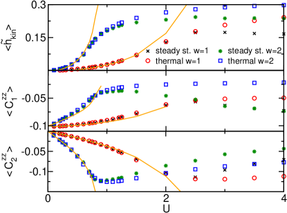
Figure 8: The same as in Fig. 6 but for the model including a next-nearest-neighbor interaction.

We perform an analysis similar to the one of the last section in the presence of the next-nearest-neighbor interaction $W$. For this model no extensive set of (quasi-) local integrals of motion is known. It is generally believed that such a set does not exist. We perform the time evolution with $H_{\rm f}=H$ of Eq. (99) with $U>0$ as well as $W=wU>0$. We show exemplary results for the steady-state and thermal expectation values of $\tilde{h}_{\rm kin}(t)$ and $C_{r}^{zz}$, with $r=1,2$, in Fig. 8. Again we find that our numerical results for $\tilde{h}_{\rm kin}(t)$ being out of the ‘thermalization class’ (as well as the ‘factor of two class’) are consistent with second order thermalization. For spin-spin correlations, not being in the ‘factor of two class’, only the leading linear order of $\left<\tilde{C}_{r}^{zz}\right>_{\rm ss}$ and $\left<\tilde{C}_{r}^{zz}\right>_{\rm th}$ agree. As for $W=0$, the quantitative agreement between thermal and steady-state expectation values of $\tilde{h}_{\rm kin}(t)$ as well as $C_{r}^{zz}$ with $r=1,2$ are surprisingly good even for interactions as large as $U=2$ ($U=1$) for $W=U$ ($W=2U$), indicating that differences in the prefactors of subleading contributions must be small.

The results of this section illustrate that leading order thermalization investigated by us is insensitive to the presence or absence of an extensive set of (known) integrals of motion.

VI Summary

A complete summary of our work on small quenches was already given in the introductory Sects. I.3 to I.7 and we here refrain from repeating this. Instead we emphasize our main results and put them into a broader perspective.

Based on analytical insights for time-averages we have developed a ‘small-quench thermalization phenomenology’ which shows that leading (nonvanishing) order thermalization of local observables and correlation functions is a ubiquitous phenomenon for quenches out of the ground state of $H_{\rm i}$. This holds independently of the number and nature of the integrals of motion inherent to a certain model as was shown by explicitly studying the quench dynamics of four distinct 1d models from different classes.

In accordance with the prethermalization conjecture the steady-state expectation value is reached in a single-step relaxation procedure and is thus unaffected by a possible second step of the dynamics of the nonlocal mode occupancies (which we did not investigate).

The more local the observable the smaller either the differences between the steady-state and thermal expectation values or the smaller the values themselves even for sizable amplitudes $g$ of the quench parameter. Both makes it very difficult to make reliable statements about thermalization for small $|g|$ based on purely computational studies (prone to numerical errors) of models which cannot be solved exactly. The heavily studied interaction quench in the XXZ-chain and related models is a particularly astonishing example for this as the steady-state and thermal expectation values of typical local observables are virtually indistinguishable in the entire metallic regime.

We start the time evolution in a pure state and the unitary dynamics implies a pure state also at large times. Thermalization of local observables can still be expected as the rest of the system can be viewed as a reservoir to the (small) subsystem which supports the observable. This argument cannot be used for the nonlocal mode occupancies and other nonlocal observables. We thus believe that our results for small quenches provide a rather satisfying picture of thermalization.

The expectation values of the observables computed in many of our model studies can be obtained from the statistical average taken with a properly chosen GGE. This is obvious for the quadratic as well as the effectively quadratic models (and mentioned in Sects. III and IV)Barthel08 ; Sotiriadis14 and, most likely, also holds true for the XXZ-chain with nearest-neighbor interaction.Pozsgay14 ; Wouters14 . This raises the question under what conditions (for which observables) a GGE prediction happens to be identical to a thermal description up to a given order in the quench amplitude. It would be very interesting to further pursue this question.

We finally emphasize that our explicit results of second order thermalization for the studied observables of 1d Fermi systems of Sects. IV and V are not at odds with earlier indications of (nonthermal) Luttinger liquid universality of the same observables in the steady state after an interaction quench.Karrasch12 ; Kennes13 The Luttinger liquid universality can be found in the large distance behavior of post-quench correlation functions while the thermal behavior is restricted to local correlation functions and observables.

- (1) A. Polkovnikov, K. Sengupta, A. Silva, and M. Vengalattore, Rev. Mod. Phys. 83, 863 (2011).
- (2) C. Gogolin and J. Eisert, Rep. Prog. Phys. 79, 056001 (2016).
- (3) I. Bloch, J. Dalibard, and W. Zwerger, Rev. Mod. Phys. 80, 885 (2008).
- (4) L. D’Alessio, Y. Kafri, A. Polkovnikov, and M. Rigol, Adv. Phys. 65, 239 (2016).
- (5) M. Moeckel and S. Kehrein, Phys. Rev. Lett. 100, 175702 (2008).
- (6) M. Moeckel and S. Kehrein, Annals of Physics 324, 2146 (2009).
- (7) P. Calabrese, F.H.L. Essler, and M. Fagotti, Phys. Rev. Lett. 106, 227203 (2011).
- (8) P. Calabrese, F.H.L. Essler, and M. Fagotti, J. Stat. Mech. P07016 (2012).
- (9) U. Schollwöck, Ann. Phys. 326, 96 (2011).
- (10) C. Karrasch and J. E. Moore, Phys. Rev. B 86, 155156 (2012).
- (11) E.A. Yuzbashyan, B.L. Altshuler, and B.S. Shastry, J. Phys. A: Math. Gen. 35, 7525 (2002).
- (12) J. Berges, S. Borsányi, and C. Wetterich, Phys. Rev. Lett. 93, 142002 (2004).
- (13) M. Eckstein, M. Kollar, and P. Werner, Phys. Rev. Lett. 103, 056403 (2009).
- (14) M. Kollar, F.A. Wolf, and M. Eckstein, Phys. Rev. B 84, 054304 (2011).
- (15) T. Giamarchi, Quantum Physics in One Dimension (New York: Oxford University Press, 2003).
- (16) K. Schönhammer in Interacting Electrons in Low Dimensions ed. by D. Baeriswyl (Dordrecht: Kluwer Academic Publishers, 2005), arXiv:cond-mat/0305035.
- (17) M.A. Cazalilla, Phys. Rev. Lett. 97, 156403 (2006).
- (18) G.S. Uhrig, Phys. Rev. A 80, 061602 (2009).
- (19) A. Iucci and M.A. Cazalilla, Phys. Rev. A 80, 063619 (2009).
- (20) J. Rentrop, D. Schuricht, and V. Meden, New J. Phys. 14, 075001 (2012).
- (21) C. Karrasch, J. Rentrop, D. Schuricht, and V. Meden, Phys. Rev. Lett. 109, 126406 (2012).
- (22) M. Fabrizio and A.O. Gogolin, Phys. Rev. B 51, 17827 (1995).
- (23) S.R. White, Phys. Rev. Lett. 69, 2863 (1992).
- (24) M. Fagotti, M. Collura, F.H.L. Essler, and P. Calabrese, Phys. Rev. B 89, 125101 (2014).
- (25) B. Pozsgay, M. Mestyán, M.A. Werner, M. Kormos, G. Zaránd, and G. Takács, Phys. Rev. Lett. 113, 117203 (2014).
- (26) B. Wouters, J. De Nardis, M. Brockmann, D. Fioretto, M. Rigol, and J.-S. Caux, Phys. Rev. Lett. 113, 117202 (2014).
- (27) E. Ilievski, J. De Nardis, B. Wouters, J.-S. Caux, F.H.L. Essler, and T. Prosen, Phys. Rev. Lett. 115, 157201 (2015).
- (28) F.H.L. Essler, H. Frahm, F. Göhmann, A. Klümper, and V.E. Korepin, The One-Dimensional Hubbard Model (Cambridge: Cambridge University Press, 2005)
- (29) M. Rigol, V. Dunjko, V. Yurovsky, and M. Olshanii, Phys. Rev. Lett. 98, 050405 (2007).
- (30) T. Barthel and U. Schollwöck, Phys. Rev. Lett. 100, 100601 (2008).
- (31) S. Sotiriadis and P. Calabrese, J. Stat. Mech., P07024 (2014).
- (32) J. von Delft and H. Schoeller, Annalen der Physik 7, 225 (1998).
- (33) D.M. Kennes and V. Meden, Phys. Rev. B 88, 165131 (2013).
- (34) V. Meden, W. Metzner, U. Schollwöck, O. Schneider, T. Stauber, and K. Schönhammer, Eur. Phys. J. B 16, 631 (2000).
- (35) S. Grap and V. Meden, Phys. Rev. B 80, 193106 (2009).
- (36) T. Deguchi, K. Fabricius, and B.M. McCoy, J. Stat. Phys. 102, 701 (2001).
- (37) M. Fagotti, J. Stat. Mech. P0301 (2014).
- (38) G. Vidal, Phys. Rev. Lett. 98, 070201 (2007).
- (39) R. Orus and G. Vidal, Phys. Rev. B 78, 155117 (2008).
- (40) F. Verstraete, J.J. García-Ripoll, J.I. Cirac, Phys. Rev. Lett. 93 207204 (2004).