Analytical expression for radial distribution function of hard sphere system:
density derivative and application to perturbation theories

Abstract

Model of hard sphere system is important part of modern theories of liquids. Radial distribution function of hard sphere fluid represented in form of explicit analytical expression allows to obtain thermodynamic potentials in analytical form, which is very helpful for further analysis and applications. A new analytical expression of radial distribution function of hard sphere fluid is developed. The density derivative of the radial distribution function and the first two terms of Barker-Henderson perturbation theory are derived as analytical expressions. The obtained results agree well with published simulation data. These results have important implications for real fluid modeling using density functional theory and perturbation theories.

I Introduction

Perturbation theories (PT) play crucial role in description of thermodynamic properties of fluids at wide range of densities Zwanzig (1954); Weeks et al. (1971); Barker and Henderson (1967a, b). General idea of these theories is the transition from complex real system to more simple reference system, which is described by the repulsive part of interaction potential. As the reference system the hard sphere (HS) fluid is commonly used Hansen and McDonald (1990).

One of the most successful PT is the one suggested by Barker-Henderson (BH) Barker and Henderson (1967a, b). This theory describes molecules as spheres of diameter $\sigma$ interacting by pair potential $U(r)$, where $r$ is the distance between centers of the molecules. In BH theory the intermolecular potential is decomposed into a sum of two piecewise functions $U(r)=U_{0}(r)+U_{1}(r)$: a reference $U_{0}$ and a perturbation $U_{1}$ term. Then, it is possible to represent the Helmholtz free energy $A$ as following series

$$A=\sum_{n=0}^{\infty}\beta^{n}A_{n},$$

where $\beta=(kT)^{-1}$, $k$ is the Boltzmann constant, $T$ is temperature, $A_{0}$ is the Helmholtz free energy of the reference fluid, $A_{n}$ is the n-th order perturbation term. Exact properties of $A_{0}$ are unknown, however, it is possible to map the reference fluid to hard spheres system with another effective diameter Barker and Henderson (1967b):

$$d=\int_{0}^{\sigma}\left(1-e^{-\beta U(r)}\right)dr<\sigma.$$

In order to describe the behavior of reference system, the theory of correlation functions is used Hansen and McDonald (1990); Barker and Henderson (1976). Thus, the only data one needs for calculation of the first term of PT $a_{1}=\beta A_{1}/N$ ($N$ is the number of molecules) is information about radial distribution function $g(r)$ (RDF) (i.e., pair correlation function):

$$a_{1}=2\pi\rho\int_{\sigma}^{\infty}g(r)U(r)r^{2}dr.$$ (1)

Description of second-order perturbation term is more complicated, since information about correlation functions of order higher then the first is needed Smith et al. (1970). However, Barker and Henderson developed compressibility approximation Barker and Henderson (1967a, b). According to this model the second term $a_{2}=\beta A_{2}/N$ is:

$$a_{2}=-\pi\rho K^{HS}\int_{\sigma}^{\infty}g(r)(U(r))^{2}r^{2}dr,$$ (2)

where $K^{HS}=kT(\partial\rho/\partial P)_{T}$ is the isothermal compressibility of reference system (HS fluid), $\rho$ and $P$ are the density and the pressure of HS fluid, respectively. Parameter $K^{HS}$ can be calculated from the density derivative of the Carnahan Starling compressibility Carnahan and Starling (1969)

$$K^{HS}=\frac{(1-\phi)^{4}}{1+4\phi+4\phi^{2}-4\phi^{3}+\phi^{4}},$$

where $\phi=\pi\rho d^{3}/6$ is the dimensionless density. Everywhere below when we say the density $\phi$. As one can see above, all the required properties of HS system can be obtained from RDF.

The initial description of HS fluid was performed by by Wertheim Wertheim (1963) and Thile Thiele (1963). They obtained the solution of Ornstein–Zernike equation in Percus-Yevick (PY) approximation Percus and Yevick (1958). However, analytical result was obtained only for the Laplace transform $G(t,\phi)$ of product $rg(r,\phi)$

$$G(t,\phi)=\int_{0}^{\infty}rg(r,\phi)e^{-tr}dr.$$ (3)

Wertheim Wertheim (1963) obtained Laplace image $G(t)$ as analytical function. According to him RDF has the following form:

$$g(r,\phi)=\frac{1}{2\pi i}\int_{\delta-i\infty}^{\delta+i\infty}\frac{tL(t,\phi)e^{tr}dt}{12\phi r\left[L(t,\phi)+S(t,\phi)e^{t}\right]},$$ (4)

where, $\delta$ is point on the real coordinate of the complex plane, such that $\delta$ is greater than the real part of all singularities of the integrand.

$$L(t,\phi)=12\phi[(1+1/2\phi)t+(1+2\phi)],$$

$$S(t,\phi)=(1-\phi)^{2}t^{3}+6\phi(1-\phi)t^{2}+18\phi^{2}t-$$ (5)

$$-12\phi(1+2\phi).$$

To obtain inverse Laplace transform, Wertheim expanded the denominator of integrand in (4) and applied residue theorem

$$g(r,\phi)=\sum_{n=1}^{\infty}\theta(r-nd)g_{n}(r,\phi),$$ (6)

where $\theta(r)$ is the Heaviside step function, and $g_{n}(r)$ is result of residue theorem defined at certain shell $nd<r<(n+1)d$. Also, Wertheim obtained $g_{1}$ in the range $d<r<2d$. Then several authors Throop and Bearman (1965); Smith and Henderson (1970); Henderson (1988) extended Wertheim’s result to wider range of RDF definitions. Later results for RDF in a same form as (6) were obtained using alternative methods by Chang and Sandler (1994); Santos (2016). These results are useful for applications, but are subject to certain limitations. Expressions for RDF defined in a wide range of $r$ are very complicated. As the result, it is not possible to obtain simple analytical expressions for (1), (2) and for the density derivative of RDF. Thus construction RDF in new form allowing, to avoid further numerical calculations is actual problem Henderson (2015); Kelly et al. (2016)

In case of HS fluid PY theory provides excellent approximation to the exact solution, and it is widely used. The accuracy problem arise in the cases of small $r$ or large $\phi$. In order to improve PY result, Verlet and Weis Verlet and Weis (1972) proposed an analytical construction, which provides new results within 1% accuracy Kalikmanov (2013).

In this paper new analytical expression for RDF is obtained. This result makes possible to make explicit integrations (1), (2) and derive their analytical expressions. Also analytical expression of the density derivative $\partial g(r,\phi)/\partial\phi$ is obtained. The results of this work are satisfied to the following points:

• HS fluid is considered as reference system for several PT, for this reason, it is necessary to know explicit expression for $g(r)$ over whole range $r>d$.

• The functional form of RDF has to be appropriate for calculation of integrals (1), (2) in convenient explicit way.

• The minimum of functional for Helmholtz free energy and the pressure are obtained by differentiation with respect to $\rho$. Thus, explicit expression for RDF derivatives is needed

II Theory

II.1 New form of RDF

In this section integral (4) is calculated by direct method using residue theorem of complex analysis. For determination of singularity points it is necessary to solve following equation in variable $t$ (denominator of (4) equals to zero):

$$F(t,\phi)=L(t,\phi)+S(t,\phi)e^{t}=0$$ (7)

after substitution of expressions (I), it transforms into transcendental equation for variable $t$:

$$12\phi[(1+1/2\phi)t+(1+2\phi)]+[(1-\phi)^{2}t^{3}+$$

$$+6\phi(1-\phi)t^{2}+18\phi^{2}t-12\phi(1+2\phi)]e^{t}=0.$$ (8)

Equation (II.1) has infinite number of roots on complex plane. Let us start with obvious root $t=0$ which is pole of the third rang, also it is unique real solution of (II.1). The other roots are conjugated complex simple poles $t_{n}=R_{n}\pm iI_{n}$, where $R_{n}$, $I_{n}$ are real and imaginary parts of complex number. Thus, in accordance to residue theorem, expression (4) can be rewritten as:

$$g(r,\phi)=1+\dfrac{d}{r}\sum\limits_{\left\{t_{n}\right\}}\dfrac{t_{n}L(t_{n},\phi)}{12\phi F^{\prime}(t_{n},\phi)}e^{t_{n}r/d}=$$

$$=1+\dfrac{d}{r}\sum\limits_{\left\{t_{n}\right\}}C_{n}(\phi)e^{t_{n}r/d},$$ (9)

where $F^{\prime}(t_{n},\phi)$ is derivative with respect to $t$ at the point $t=t_{n}$, here the first term “1”corresponds to the residue at point $t=0$, the second term is sum over all simple complex poles. Simpler expression can be obtained after summing conjugated poles:

$$g(r,\phi)=1+\dfrac{2d}{r}\sum\limits_{n=1}^{\infty}A_{n}(\phi)e^{R_{n}r/d}\cos(I_{n}r/d+\alpha_{n}),$$

where

$$A_{n}=\left|\dfrac{t_{n}L(t_{n},\phi)}{12\phi F^{\prime}(t_{n},\phi)}\right|,\,\,\,\ \alpha_{n}=\arg\left(\dfrac{t_{n}L(t_{n},\phi)}{12\phi F^{\prime}(t_{n},\phi)}\right).$$

Expression (II.1) contains only real functions which are depended on $\phi,t_{n}$. Thus, as one can see from (II.1), in order to calculate RDF, the distributions of roots $t_{n}(\phi)$ is only needed.

Let us consider new equation which is the limit $|t|\to\infty$ of equation (II.1):

$$12\phi(1+1/2\phi)+(1-\phi)^{2}z^{2}e^{z}=0$$ (12)

By introduction of a new variable $q=-\frac{12\phi(1+1/2\phi)}{(1-\phi)^{2}}$ it is possible to rewrite (12) in more simple form: $z^{2}e^{z}=q$. Such equation can be solved exactly in terms of Lambert functions $W(x)$ Scott et al. (2006); Corless et al. (1996)

$$W(x)e^{W(x)}=x.$$

After simple modifications, the above equation can be written as $(2W(x))^{2}e^{2W(x)}=4x^{2}$. Thus, solution of equation (12) has the following form

$$z_{n}=2W(n,\pm q^{1/2}/2),$$ (13)

where $n=1,2,...$ enumerates complex branch of Lambert function.

Using exact solution (13) as the limit, the solution of (II.1) can be written as series of $z_{n}^{-1}$:

$$t_{n}=z_{n}+\sum_{k=1}^{\infty}a_{k}z_{n}^{-k}$$ (14)

where coefficients $a_{n}$ depend only on density $\phi$ and can be found after substitution of (14) in (II.1). In this work four terms were calculated, in Fig. 1 one can see typical distribution of the poles on upper half complex plane (down half plane looks same, but symmetry reflected). From this figure and Table 1, one can see that analytical expression with 4 terms (14) is accurate approximation for numerical solutions of (II.1).

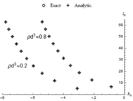
Figure 1: Typical distribution of the poles in the upper half complex plane. Circle points correspond to numerical solution (II.1), cross points are results of analytical expression with 4 terms (14).

Table 1: Comparison of real $R_{1}$ and imaginary $I_{1}$ parts of first root $t_{1}$ which are calculated by numerical results for (II.1) (“Exact”-column) and by analytical expression (14) with 4 terms (“Analytic.”-column). Results are obtained for several densities, relative deviation is not biger than 1%.

$\rho d^{3}$	Exact $R_{1}$	Exact $I_{1}$	Analytic. $R_{1}$	Analytic. $I_{1}$
0.1	-4.072	4.761	-4.072	4.761
0.3	-2.487	5.398	-2.482	5.396
0.5	-1.667	5.889	-1.650	5.901
0.7	-1.089	6.351	-1.079	6.418

For the aims of this work it will be enough to consider only one term in the sum (14). Here and below following expression is used as approximations for the roots of (II.1):

$$t_{n}\simeq z_{n}+\frac{2(1-5\phi+5\phi^{2})}{(1-\phi)(2+\phi)}z_{n}^{-1}$$ (15)

It is easy to verify, that for all poles $R_{n}=Re(t_{n})<0$, and $R_{n+1}<R_{n}$, then contribution of exponential n-th term in sum (II.1) rapidly decreases, when the number $n$ increases. Thus, for accurate result summation over all terms in (II.1) is not required and (II.1) can be rewritten as analytical expression with $M$ terms:

$$g(r)=1+\frac{2d}{r}\sum_{n=1}^{M}A_{n}(\phi)e^{R_{n}r/d}\cos(I_{n}r/d+\alpha_{n}).$$ (16)

Accurate result for the point of contact ($r=d$) requires summation over large number of terms (poles). This effect is well known in inverse Laplace or Fourier transforms and is called “Gibbs phenomenon”. Non-formally there is the overestimate in value of finite series near the point of function jump ($g(r)$ near $r=d$). This artifact appears when discontinuous function approximated by finite series of continuous functions. Amplitude of the overestimate does not disappear as $M$ increases, and tends to finite value. However infinite limit of series does not the overestimates, because the location of the overestimate moves aside point of function discontinuity. In other words, there is pointwise convergence, but not uniform convergence Pinsky (2002). Practical result can be found as $g(d)\simeq g(d+\epsilon(M))$, where $\epsilon\ll d$ and $\epsilon\to 0$ when $M\to\infty$. Solid and dashed curves in Fig. 2 correspond to $M=1000$. In this figure one can see, that comparison of analytical expression (16) and numerical results Throop and Bearman (1965) demonstrates good accuracy. For further calculations it is enough to use only $M=100$ terms in (16).

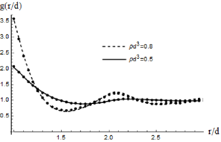
Figure 2: PY RDF as function of dimensionless distance $r/d$ calculated for two cases of density $\rho d^{3}=0.8,\rho d^{3}=0.6$, dashed and solid lines, respectively. Points correspond to published numerical data Throop and Bearman (1965).

In spite of wide applications, PY approximation has two weak points: the contact value $g(d)$ is too low at high density; phase of oscillation at large distance $r$ differs from the exact one. In order to correct these artifacts construction of Verlet-Weis can be used Verlet and Weis (1972). This is achieved by introduction of a modified density $\phi_{m}=\phi+\phi^{2}/16$ and modified HS diameter $d_{m}=\left(\phi_{m}/\phi\right)^{1/3}d$ in order to correct RDF oscillation. Verlet and Weis, also, proposed an addition term which improved contact value $g(d)$, so corrected RDF has following form:

$$g^{VW}(r/d)=g(r/d_{m};\phi_{m})+\dfrac{1}{r}e^{\frac{\alpha(r-d)}{d}}\cos\dfrac{\alpha(r-d)}{d},$$

where parameters $A$ and $\alpha$ can be found from

$$\dfrac{A}{d}=\dfrac{3}{4}\dfrac{\phi_{m}(1-0.7117\phi_{m}-0.114\phi_{m}^{2})}{(1-\phi_{m})^{4}}$$

$$\alpha=\dfrac{24A/d}{\phi_{m}g(d_{m},\phi_{m})}$$

The form of expression of added term in (II.1) coincides with analytical result (II.1). This fact helps the process of further calculations of corrected form (II.1).

After application of VW procedure the obtained RDF can be compared with the results of HS modeling. Fig. 3 demonstrates, that analytical expression (II.1) for M=100 with VW corrections correctly describes the behavior of HS fluid.

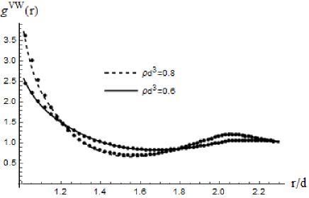
Figure 3: Corrected RDF (II.1) as function of dimensionless distance $r/d$ calculated for two cases of density: $\rho d^{3}=0.8,\rho d^{3}=0.6$, dashed and solid lines, respectively. Points correspond to published data of Monte Carlo simulations Barker and Henderson (1971)

It is important to note that approximated expressions for singularities of (4) were investigated in Perram and Smith (1980). However, in previous works exact solution of (12) has never been implemented. The exact solution of (12) is required to obtain right expression for derivative $\partial g(r,\phi)/\partial\phi$.

II.2 Density derivative of RDF

The method proposed in this work allows to obtain the density derivative of RDF without decrease of accuracy. It follows from the fact that all variables of (II.1) are explicit functions of density, so all partial derivatives can be written as analytical expressions.

$$\frac{\partial g(r,\phi)}{\partial\phi}=\frac{1}{r}\sum_{n}\left[\frac{\partial C_{n}}{\partial\phi}+\frac{\partial C_{n}}{\partial t_{n}}\frac{\partial t_{n}}{\partial\phi}+rC_{n}\frac{\partial t_{n}}{\partial\phi}\right]e^{t_{n}r},$$

where derivative $\partial t_{n}/\partial\phi$ can be calculated exactly using properties of Lambert function Corless et al. (1996)

$$\frac{\partial W_{n}(x)}{\partial x}=\frac{1}{x}\frac{W_{n}(x)}{W_{n}(x)+1}.$$

This relationship is correct for any branch of Lambert function. Thus,

$$\dfrac{\partial z_{n}}{\partial\phi}=\dfrac{1}{q}\dfrac{W_{n}(\pm q^{1/2}/2)}{W_{n}(\pm q^{1/2}/2)+1}\frac{\partial q}{\partial\phi}=$$

$$=\dfrac{-1-2\phi}{\sqrt{6}(-\phi(2+\phi))^{3/2}}\dfrac{z_{n}}{z_{n}+2}.$$

II.3 Perturbation terms

Analytical expressions of RDF play important role in calculation of perturbation terms. Indeed, numerical integrations of (1) and (2) at each density is inconvenient. The derived above expression for RDF of HS makes it possible to obtain the perturbation terms in analytical form. Also analytical integrated expressions (1), (2) can be used in equation of state for real fluid and density functional theory calculations.

Let us consider the system of molecules interacting by potential

$$U(r)=\epsilon\gamma\left[\left(\frac{\sigma}{r}\right)^{\lambda_{r}}-\left(\frac{\sigma}{r}\right)^{\lambda_{a}}\right],$$

where $\epsilon$ is characteristic energy, $\gamma=\frac{\lambda_{r}}{\lambda_{r}-\lambda_{a}}\left(\frac{\lambda_{r}}{\lambda_{a}}\right)^{\frac{\lambda_{r}}{\lambda_{r}-\lambda_{a}}}$ is a constant, which in case of Lennard-Jones (LJ) fluid ($\lambda_{r}=12,\lambda_{a}=6$) equals to $\gamma=4$. Then, at certain temperature $T$ for Barker-Henderson PT the reference system is a system of HS molecules with diameter $d(T)<\sigma$. Thus, the first two terms of PT are defined by RDF of HS molecules with known diameter $d$. Using the explicit spatial dependence of RDF $g^{VW}(r)$ (II.1), all necessary integrals can be expressed in the following general form:

$$\int_{x_{0}}^{\infty}\frac{dr}{r^{n}}e^{ar}=x_{0}^{-n+1}E_{n}(-ax_{0})$$ (18)

where $E_{n}(x)$ is the exponential integral Gradshteyn and Ryzhik (2014). After substitution of RDF $\eqref{RDF_VW}$ into (1) and (2), the first and the second terms of PT are

$$a_{1}(\phi)=12\gamma\epsilon\phi\left\{\dfrac{x_{0}^{3}}{\lambda_{r}-1}+\dfrac{x_{0}^{3}}{\lambda_{a}-1}+\dfrac{x_{0}^{2}}{k}\sum_{n}C_{n}\left[E_{\lambda_{r}-1}(-kx_{0}t_{n})+E_{\lambda_{a}-1}(-kx_{0}t_{n})\right]+\right.$$ (19)

$$\left.+\dfrac{x_{0}^{2}A}{2}\left[E_{\lambda_{r}-1}(-x_{0}\tau)+E_{\lambda_{r}-1}(-x_{0}\tau^{*})+E_{\lambda_{a}-1}(-x_{0}\tau)+E_{\lambda_{a}-1}(-x_{0}\tau^{*})\right]\right\}$$

$$a_{2}(\phi)=-6\gamma^{2}\epsilon^{2}\phi K\bigg{\{}\dfrac{x_{0}^{3}}{2\lambda_{r}-1}-\dfrac{2x_{0}^{3}}{\lambda_{r}+\lambda_{a}-1}+\dfrac{x_{0}^{3}}{2\lambda_{a}-1}+$$

$$+\dfrac{x_{0}^{2}}{k}\sum_{n}C_{n}\left[E_{2\lambda_{r}-1}(-kx_{0}t_{n})-2E_{\lambda_{r}+\lambda_{a}-1}(-kx_{0}t_{n})+E_{2\lambda_{a}-1}(-kx_{0}t_{n})\right]+$$ (20)

$$+\dfrac{x_{0}^{2}A}{2}\left[E_{2\lambda_{r}-1}(-x_{0}\tau)+E_{2\lambda_{r}-1}(-x_{0}\tau^{*})-2E_{\lambda_{r}+\lambda_{a}-1}(-x_{0}\tau)-\right.$$

$$\left.-2E_{\lambda_{r}+\lambda_{a}-1}(-x_{0}\tau^{*})+E_{2\lambda_{a}-1}(-x_{0}\tau)+E_{2\lambda_{a}-1}(-x_{0}\tau^{*})\right]\bigg{\}}$$

where $\tau=-\alpha+i\alpha$ and conjugated one $\tau^{*}=-\alpha-i\alpha$. Taking into account expression (15), results (19),(II.3) are analytical expressions with explicit dependence on the density $\phi$. Fig. 4 shows the dependence on density $\rho\sigma^{3}$ of $a_{1}$ for LJ fluid at temperature $T=\epsilon/k$ . As one can see, analytical expression (19) (solid line) demonstrates excellent agreement with Monte Carlo simulations (dots) Lafitte et al. (2013).

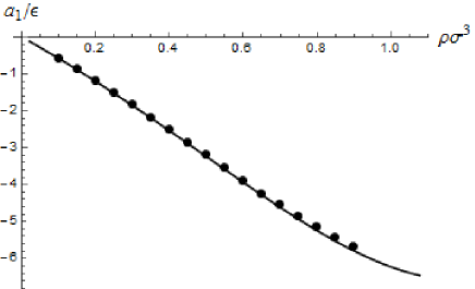
Figure 4: The density $\rho\sigma^{3}$ dependence of the first perturbation terms for the LJ system at temperature $T=\epsilon/k$. Solid curve is analytical result (19), dots correspond to Monte Carlo simulations Lafitte et al. (2013)

.

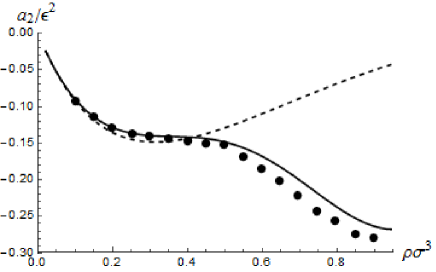
Figure 5: The density $\rho\sigma^{3}$ dependence of the second perturbation terms for the LJ system at temperature $T=\epsilon/k$. Dashed curve corresponds to analytical result (II.3) without correction prefactor $\chi=0$. Solid curve is analytical result (II.3) taking into account correction prefactor from work Lafitte et al. (2013). Dots correspond to Monte Carlo simulations Lafitte et al. (2013).

In case of the second term $a_{2}$, the comparison with simulation data is more complicated. Definition (2) is approximated result and corresponds to “compressibility approximation”of BH. How one can see from Fig. 5, result (II.3) without correction prefactor (dashed line) works well only for low range of densities. Better version of correction prefactor $1+\chi$ was implemented in work Lafitte et al. (2013). With account of this $\chi$ from work Lafitte et al. (2013), expression (II.3) matches numerical data in whole range of the densities, solid line in Fig. 5.

III Conclusion

In this work analytical expression for inverse Laplace transform of Wertheim’s result was calculated. This expression was represented as the sum of the residues at the simple poles. Exact expressions for the complex poles were found in terms of Lambert function. Accurate results were obtained by appropriate approximations for poles and the overall sum. After Verlet-Weis corrections this result can be applied to description of hard sphere fluid. Also the density derivative, and two first terms of Barker-Henderson perturbation theory were calculated. All obtained results coincide well with published results of Monte Carlo simulations. Results of this work have important implications for modeling of real fluids by density functional methods and perturbation theories.

References

- Zwanzig (1954) R. W. Zwanzig, The Journal of Chemical Physics 22, 1420 (1954).
- Weeks et al. (1971) J. D. Weeks, D. Chandler, and H. C. Andersen, The Journal of chemical physics 54, 5237 (1971).
- Barker and Henderson (1967a) J. A. Barker and D. Henderson, The Journal of Chemical Physics 47, 2856 (1967a).
- Barker and Henderson (1967b) J. A. Barker and D. Henderson, The Journal of Chemical Physics 47, 4714 (1967b).
- Hansen and McDonald (1990) J.-P. Hansen and I. R. McDonald, Theory of simple liquids (Elsevier, 1990).
- Barker and Henderson (1976) J. A. Barker and D. Henderson, Reviews of Modern Physics 48, 587 (1976).
- Smith et al. (1970) W. Smith, D. Henderson, and J. Barker, Journal of Chemical Physics 53, 508 (1970).
- Carnahan and Starling (1969) N. F. Carnahan and K. E. Starling, The Journal of Chemical Physics 51, 635 (1969).
- Wertheim (1963) M. Wertheim, Physical Review Letters 10, 321 (1963).
- Thiele (1963) E. Thiele, The Journal of Chemical Physics 39, 474 (1963).
- Percus and Yevick (1958) J. K. Percus and G. J. Yevick, Physical Review 110, 1 (1958).
- Throop and Bearman (1965) G. J. Throop and R. J. Bearman, The Journal of Chemical Physics 42, 2408 (1965).
- Smith and Henderson (1970) W. Smith and D. Henderson, Molecular Physics 19, 411 (1970).
- Henderson (1988) D. Henderson, Journal of colloid and interface science 121, 486 (1988).
- Chang and Sandler (1994) J. Chang and S. I. Sandler, Molecular Physics 81, 735 (1994).
- Santos (2016) A. Santos, in A Concise Course on the Theory of Classical Liquids (Springer, 2016) pp. 203–253.
- Henderson (2015) D. Henderson, Molecular Physics , 1 (2015).
- Kelly et al. (2016) B. D. Kelly, W. R. Smith, and D. Henderson, Molecular Physics , 1 (2016).
- Verlet and Weis (1972) L. Verlet and J.-J. Weis, Physical Review A 5, 939 (1972).
- Kalikmanov (2013) V. Kalikmanov, Statistical physics of fluids: basic concepts and applications (Springer Science & Business Media, 2013).
- Scott et al. (2006) T. C. Scott, R. Mann, and R. E. Martinez Ii, Applicable Algebra in Engineering, Communication and Computing 17, 41 (2006).
- Corless et al. (1996) R. M. Corless, G. H. Gonnet, D. E. Hare, D. J. Jeffrey, and D. E. Knuth, Advances in Computational mathematics 5, 329 (1996).
- Pinsky (2002) M. A. Pinsky, Introduction to Fourier analysis and wavelets, Vol. 102 (American Mathematical Soc., 2002).
- Barker and Henderson (1971) J. Barker and D. Henderson, Molecular Physics 21, 187 (1971).
- Perram and Smith (1980) J. Perram and E. Smith, Journal of Physics A: Mathematical and General 13, 2219 (1980).
- Gradshteyn and Ryzhik (2014) I. S. Gradshteyn and I. M. Ryzhik, Table of integrals, series, and products (Academic press, 2014).
- Lafitte et al. (2013) T. Lafitte, A. Apostolakou, C. Avendano, A. Galindo, C. S. Adjiman, E. A. Müller, and G. Jackson, The Journal of chemical physics 139, 154504 (2013).