STASH: Securing transparent authentication schemes using prover-side proximity verification

Abstract

Transparent authentication (TA) schemes are those in which a user is authenticated by a verifier without requiring explicit user interaction. By doing so, those schemes promise high usability and security simultaneously. The majority of TA implementations rely on the received signal strength as an indicator for the proximity of a user device (prover). However, such implicit proximity verification is not secure against an adversary who can relay messages over a larger distance.

In this paper, we propose a novel approach for thwarting relay attacks in TA schemes: the prover permits access to authentication credentials only if it can confirm that it is near the verifier. We present STASH, a system for relay-resilient transparent authentication in which the prover does proximity verification by comparing its approach trajectory towards the intended verifier with known authorized reference trajectories. Trajectories are measured using low-cost sensors commonly available on personal devices. We demonstrate the security of STASH against a class of adversaries and its ease-of-use by analyzing empirical data, collected using a STASH prototype. STASH is efficient and can be easily integrated to complement existing TA schemes.

I Introduction

User authentication is necessary in order to regulate access to data or physical objects. The predominant approach still relies on the use of passwords which suffers from drawbacks in terms of both usability and security [3]. Effective and secure alternatives to password-based authentication have yet to emerge [2]. This has sparked the development of transparent authentication (TA) with systems exploiting characteristic cues such as behavior [31], biometrics [25], or environmental context [28]. Zero-interaction authentication (ZIA) is a class of TA schemes [5] that relies on a verifier $\mathcal{V}$ to authenticate a user when a prover device $\mathcal{P}$ associated with the user is nearby. In ZIA schemes $\mathcal{V}$ typically verifies the proximity of $\mathcal{P}$ by measuring either the strength of radio signals emitted from $\mathcal{P}$ over some short range wireless channel, e.g. BlueProximity [24], or the time required to transmit messages over that channel, e.g. “keyless entry and start” systems for cars. However, these TA schemes remain vulnerable to relay attacks [9, 10], where the attacker relays messages between $\mathcal{P}$ and $\mathcal{V}$ when they are not co-located, leading to $\mathcal{V}$ falsely concluding that $\mathcal{P}$ is nearby.

There are several known defense techniques against these attacks such as distance bounding protocols [4] and comparison of ambient contexts between $\mathcal{P}$ and $\mathcal{V}$ [11, 28]. However, these methods are faced with deployment challenges. In effect, context-based relay attack defense systems have unclear security guarantees [23]. Additionally, distance bounding methods require precise timing, and 1 ns measurement error can affect the estimated distance by 30 cm. Therefore, additional hardware and low-level software changes seem necessary.

In this paper we propose a novel approach to thwart relay attacks on proximity-based transparent authentication systems. We present STASH, a system that enforces proximity verification by $\mathcal{P}$ to an intended $\mathcal{V}$ before allowing access to the credentials used in the authentication protocol. The method uses $\mathcal{P}$’s on-board micro-electromechanical system (MEMS) sensors to measure its approach trajectory towards $\mathcal{V}$ and compares it with authorized reference paths. A central design principle in STASH is to rely only on sensors monitoring $\mathcal{P}$’s own movement (e.g. accelerometer and gyroscope) rather than on sensors that measure environmental factors that can be manipulated or falsified (e.g. GPS, radio signal emission, or ambient properties). We built STASH as an Android application and used it to gather trajectory data of 20 different routes in two cities (totaling 123 km). Using this dataset, we demonstrate that STASH has acceptable false reject (FRR) and false accept (FAR) rates.

Commodity devices provide low-cost MEMS sensors that are noisy, include bias terms and miss data. Designing STASH to work on commodity devices raised several technical challenges leading to questions like “how to effectively represent a trajectory using only accelerometer/gyroscope measurements?” and “how to best compare two trajectories?”. Additionally, an energy budget examination of portable devices is necessary to understand the feasibility of STASH. In this paper, we address these challenges and evaluate the resulting system systemically. Briefly, our contributions are the following:

• We propose using prover-side proximity verification to resist relay attacks against proximity-based transparent authentication systems (Sections II and III).

• We design and implement a concrete system, STASH, incorporating this idea by addressing several challenges in measuring prover’s approach trajectory and using it to determine proximity to verifier (Section III).

• By systematically analyzing trajectory data in two cities, we demonstrate the security and usability of STASH (Section IV). We also show that STASH’s average energy consumption is low: we estimate that under typical usage conditions, the battery drain due to STASH over the course of a work day is in the range of 4%-7% of battery capacity. (Section IV-G).

II Concept and Assumptions

II-A System Model

Figure 1 illustrates the basis of proximity-based transparent authentication. The goal of this model is to enable confirmation from the verifier $\mathcal{V}$ that a user $\mathcal{U}$ is nearby. For this purpose, $\mathcal{U}$ has a personal device $\mathcal{P}$ and authentication is then based on a challenge-response protocol using a previously established security association, e.g. a shared symmetric key between $\mathcal{P}$ and $\mathcal{V}$. However, in addition to verifying authenticity of $\mathcal{P}$, $\mathcal{V}$ also verifies its proximity to $\mathcal{P}$, a process which is vulnerable to relay attacks.

Figure 1: Transparent authentication: challenge-response protocol triggered upon sensing proximity of $\mathcal{P}$ to $\mathcal{V}$. The proximity verification component introduced in our approach is shown as a red dashed box.

To protect against those attacks, we improve this model by having $\mathcal{P}$ regulate access to the authentication credentials through first verifying its proximity to $\mathcal{V}$. In particular, we propose that $\mathcal{P}$ does this proximity verification by examining its approach trajectory towards $\mathcal{V}$. If proximity verification fails, $\mathcal{U}$ is asked to explicitly confirm she is near $\mathcal{V}$.

Application scenario: premise access control. We target a scenario where a person $\mathcal{U}$ accompanied by $\mathcal{P}$ routinely approaches an access controlling barrier $\mathcal{V}$. After transparently authenticating $\mathcal{P}$, $\mathcal{V}$ will open the barrier to let $\mathcal{U}$ pass. If proximity verification fails, $\mathcal{U}$ may still open the gate through explicit proximity confirmation using $\mathcal{P}$. Examples for such scenario are: a person $\mathcal{U}$ on a vehicle $\mathcal{P}$ such as a bicycle, wheelchair or car requiring easy and fast access through a gate or door $\mathcal{V}$ at her home or workplace.

II-B Adversary Model

We consider an adversary $\mathcal{A}$ who has deployed a wireless relay providing him with Dolev-Yao [6] capabilities. Although $\mathcal{A}$ can control the message flow between $\mathcal{P}$ and $\mathcal{V}$, he cannot break the cryptographic protection of a secured channel. Nevertheless, by relaying the challenge and response and thus artificially extending the range of the wireless channel, $\mathcal{A}$ can successfully bypass the proximity verification since $\mathcal{V}$ will be measuring the relay device’s signal strength rather than $\mathcal{P}$’s. Even if time of flight is used to estimate the distance, off-the-shelf hardware is not precise enough to provide a secure estimate of the distance between two devices. Attacks like this are actively being exploited as demonstrated for several scenarios [9, 10].

We do not consider adversaries who gain physical access to $\mathcal{P}$. Continuous user authentication techniques, such as biometric authentication [20] can ensure it is the legitimate user who is in possession of the the device. We also assume that the device has not been infected with malware which can be ensured using platform security and anti-malware tools.

II-C Design Goals and Challenges

Goals. We set the following goals for our relay-resilient proximity verification system:

1. Usability: Transparent authentication must minimize explicit user action. If trajectory comparison fails when $\mathcal{U}$ is in fact near $\mathcal{V}$, $\mathcal{U}$ will be required to fall back to explicit proximity confirmation. Our system should therefore minimize the false reject rate.

2. Security: The system should not incorrectly conclude that $\mathcal{U}$ is near $\mathcal{V}$ even in the presence of a relay. Therefore it should minimize the false accept rate.

3. Efficiency: The computational and energy costs of proximity verification should be small to not diminish the user experience.

4. No external signals: Since $\mathcal{A}$ can control ambient properties, proximity verification should not depend on any external signals.

5. Local decision-making: Proximity verification must be carried out entirely within $\mathcal{P}$.

There are two rationales for R5. One is privacy: data collected for proximity verification should not be exposed to any third party. The other is deployability: a local solution can be seamlessly integrated into any proximity-based transparent authentication scheme by only modifying $\mathcal{P}$ without having to change the protocol and thus the implementation of $\mathcal{V}$.

III STASH Architecture

We now describe STASH, our system that uses prover-side proximity verification to prevent relay attacks.

III-A Trajectory Representation

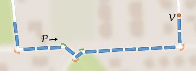
Figure 2: $\mathcal{P}$’s approach trajectory towards $\mathcal{V}$ is described by a set of primitives needed to reach $\mathcal{V}$. In this example, the primitives are move 2, left 90^∘, move 3, right 30^∘, move 1, left 90^∘, move 1, right 30^∘, move 7, left 90^∘, move 2.

To satisfy requirement R4, we avoid external, insecure, data sources like GPS [26] or ambient sensor modalities and rely only on gyroscope and accelerometer to capture user’s movement. We represent a trajectory as a temporally ordered sequence of discrete primitives consisting of segments of movement interleaved with left or right turns derived from angular information. (See Figure 2 for an example.)

An intuitive way to represent a trajectory is as a sequence of coordinates, like in dead reckoning [15]. However, a one-dimensional sequence of primitives is more robust to sensor noise than a two-(or even three-) dimensional coordinate: the impact of a missed turn on the resulting sequence is less than it is on the result of a dead reckoning algorithm.

Using sensor data, we recognize two streams of primitives: $(M/S,t_{i})$ symbols (for “movement” or “stationary” at time $t_{i}$) are generated at a fixed rate and $(L/R,t_{i})$ symbols (turn “left” or “right” at time $t_{i}$) are generated opportunistically whenever a turn is detected. The two streams are then combined into one sequence, with turn events taking precedence. The overall system has three essential parts: primitive generation, trajectory comparison and authorized trajectory updating.

III-B Primitive Generation

Turn primitives. By exploring different sampling rates and sensors, we concluded that a 20 Hz sampling rate is sufficient to detect turns with a precision of 15^∘. To achieve this, we project the gyroscope to ground direction, obtain the heading angle by integrating the angular speed and then record turns when the 2s sliding window standard deviation of the heading angle is above a threshold ($\sigma_{1}=3^{\circ}$). However, sudden gravity shifts cause errors in turn estimation: we disregard gyroscope data as unreliable in such situations. To remove drift in MEMS gyroscopes, we use a high-pass filter, where gyroscope measurements smaller than $8.6^{\circ}$/s are exponentially weighted down. Fine-grained beginnings and ends of turns are found where the sliding window standard deviation is above a smaller threshold ($\sigma_{2}=1^{\circ}$). The turn detection system assumes that $\mathcal{P}$ has reliable gravity estimates: $\mathcal{P}$ could for instance be integrated into a vehicle or firmly attached to the body to avoid disturbing the gravity direction. In this paper we collect data by integrating $\mathcal{P}$ with a bicycle.

Movement primitives. To identify movement, we use a logistic regression (LR) algorithm [17] that continuously predicts movement mode at one second intervals. The prediction is done on-the-spot, and does not take previous prediction results into account. In reality however, two successive events are dependent. We additionally use a Hidden Markov Model (HMM) [7] to capture this dependency.

In HMMs, probabilities to move between hidden states are modeled with a first-order Markov chain. Each hidden state gives a cue about itself by emitting a primitive at any given time. In our case, we want to determine movement primitives ($M$ or $S$) by observing the output of LR. We use HMM Viterbi algorithm [7] to smoothen the observations into the most likely sequence of primitives. Finally, we determine the representative primitive for each five measurements as the most frequent among the five. This scheme gives us a continuous stream of one $M$ or $S$ primitive in five seconds intervals.

III-C Trajectory Comparison

We differentiate between two types of trajectories. Reference paths are previously authorized trajectories of a $\mathcal{P}$ towards some verifier $\mathcal{V}$. Candidate paths are trajectories towards $\mathcal{V}$ perceived by $\mathcal{P}$ before a proximity verification session. These can contain errors introduced through noisy measurements. To verify proximity to $\mathcal{V}$, $\mathcal{P}$ compares the candidate path to the reference path. Figure 3 shows our proposed proximity verification scheme. If the trajectory comparison succeeds, $\mathcal{P}$ continues with the authentication protocol by computing the response to the challenge and sending it to $\mathcal{V}$. If trajectory comparison fails, the system falls back to explicit proximity confirmation by $\mathcal{U}$. Successful explicit confirmation implies that $\mathcal{P}$’s candidate path can be added to the trajectory repository as an authorized trajectory: a reference path.

Figure 3: Prover-side proximity verification. $\mathcal{P}$ compares the current candidate path against reference paths in the repository. $\mathcal{P}$ computes the response to $\mathcal{V}$’s challenge if the candidate path matches a reference path. The user is asked for explicit proximity confirmation if this check fails.

Candidate and reference paths are represented as sequences of characters as discussed in Section III-A. Trajectory comparison is therefore a similarity comparison between strings. We evaluated several string matching metrics and chose to use Needleman-Wunsch (NW) similarity [7], which is a combination of the longest common sub-sequence and edit distance algorithms. In NW terminology, both insertions and deletions are called gaps. We chose the parametrization: match +1, mismatch -2 and gap -1. Matches can be seen as evidence and mismatches counter-evidence that two sequences are related. Before comparison, $S$ symbols are removed and timestamps ($t_{i}$) are used to trim strings to the same temporal length.

Instances of the same reference path will differ due to noise from various sources. Therefore, we need to establish a decision threshold that determines how much noise is acceptable. If the similarity score is higher than the threshold, the candidate path is accepted. Otherwise it is rejected. This introduces a trade-off between usability (FRR) and security (FAR). An initial threshold that has a good FAR/FRR trade-off is determined prior to deployment as discussed in Section IV-D.

III-D Updating Reference Paths

Once the system is deployed, we use feedback from failed and successful trajectory comparison attempts to adjust the decision threshold. The initial threshold might under- or overestimate the variation in future instances of a given reference path $r$. The decision threshold should be adjusted to achieve a better FAR/FRR trade-off, either by decreasing (better usability) or increasing (better security) it.

We call such a path-specific decision threshold a local threshold. To compute local thresholds for a given $r$ we need instances $i_{r}$ of $r$ and instances $i_{\bar{r}}$ of reference paths towards other verifiers $\bar{\mathcal{V}}$. These are used to calculate within- and between-class similarities. When a user $\mathcal{U}$ starts using STASH we do not have enough instances $i_{r}$, $i_{\bar{r}}$ to compute within- and between-class similarities. Instances $i_{r}$ will be gradually collected as the user repeatedly traverses $r$. We consider two ways to acquire instances $i_{\bar{r}}$ of paths towards another $\bar{\mathcal{V}}$:

• Use trajectories generated from a map for the current geographic region.

• Collect all trajectories of a given user and create a generative probabilistic model (Markov chain) to simulate new reference paths instances.

We choose the latter option in STASH. In the beginning, STASH will only observe a few instances of a reference path and any new local decision threshold we obtain would be severely over-learned. Naively trusting the seen instances risks a small sample size fallacy. Therefore, we need a way to model the trustworthiness of the estimated local threshold. We model the confidence as a mixture model using a convex combination [17] of the thresholds $d_{i}$ (initial) and $d_{l}$ (local) with a confidence factor $\lambda\in[0,1]$:

$$d=\lambda d_{l}+(1-\lambda)d_{i}.$$ (1)

We call the resulting threshold $d$ a mixed threshold. A common way to model the confidence in small sample sizes is to use add-one smoothing [17]. When $n$ is the number of seen instances of a reference path, we can model $\lambda$ as:

$$\lambda(n)=\dfrac{n-1}{n}.$$ (2)

This fulfills our boundary conditions for $\lambda$: $\lambda(1)=0$, implies no confidence when we have only seen one instance of a reference path and $\lambda(\infty)=1$, signifying full confidence with infinitely many instances. Figure 4 shows how the confidence factor increases w.r.t. the number of reference path instances seen so far. We use equations 1 and 2 to determine mixed thresholds throughout this paper. The three thresholds mixed, local and initial are evaluated in Section IV-F.

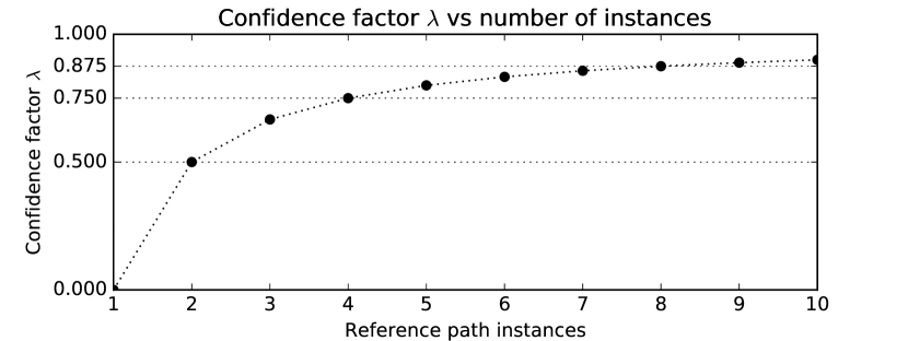
Figure 4: The confidence factor $\lambda$ increases with the number of observed reference path instances. The distance to one halves at every multiple of two.

IV Implementation and Evaluation

To be able to evaluate the performance and resource requirements of STASH under real-world conditions, we implemented our system on Android (See Figure 8).

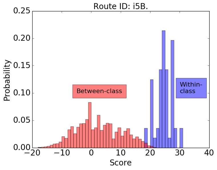
Figure 5: An example of within-class (blue) and between-class similarities (red) for one route. Choosing a reference path-specific threshold 18 minimizes equal error rate (EER) on this route.

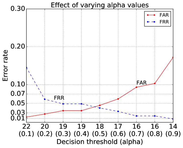
Figure 6: Error rates vs. $\alpha$ (with corresponding decision threshold). Large $\alpha$ values result in low FRR, while small $\alpha$ results in low FAR.

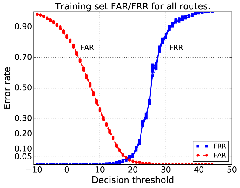
Figure 7: Training set FAR (red) and FRR (blue) for 20 routes (20 graphs). Training set for each route consists of paths of all other routes pooled together. EER is achieved at 18 in all graphs.

IV-A Prototype for STASH

To optimize power consumption, the device enters sleep after being stationary for 5 minutes. STASH acquires a wakelock [1] when significant motion is detected to ensure that no relevant sensor data is lost due to power optimization.

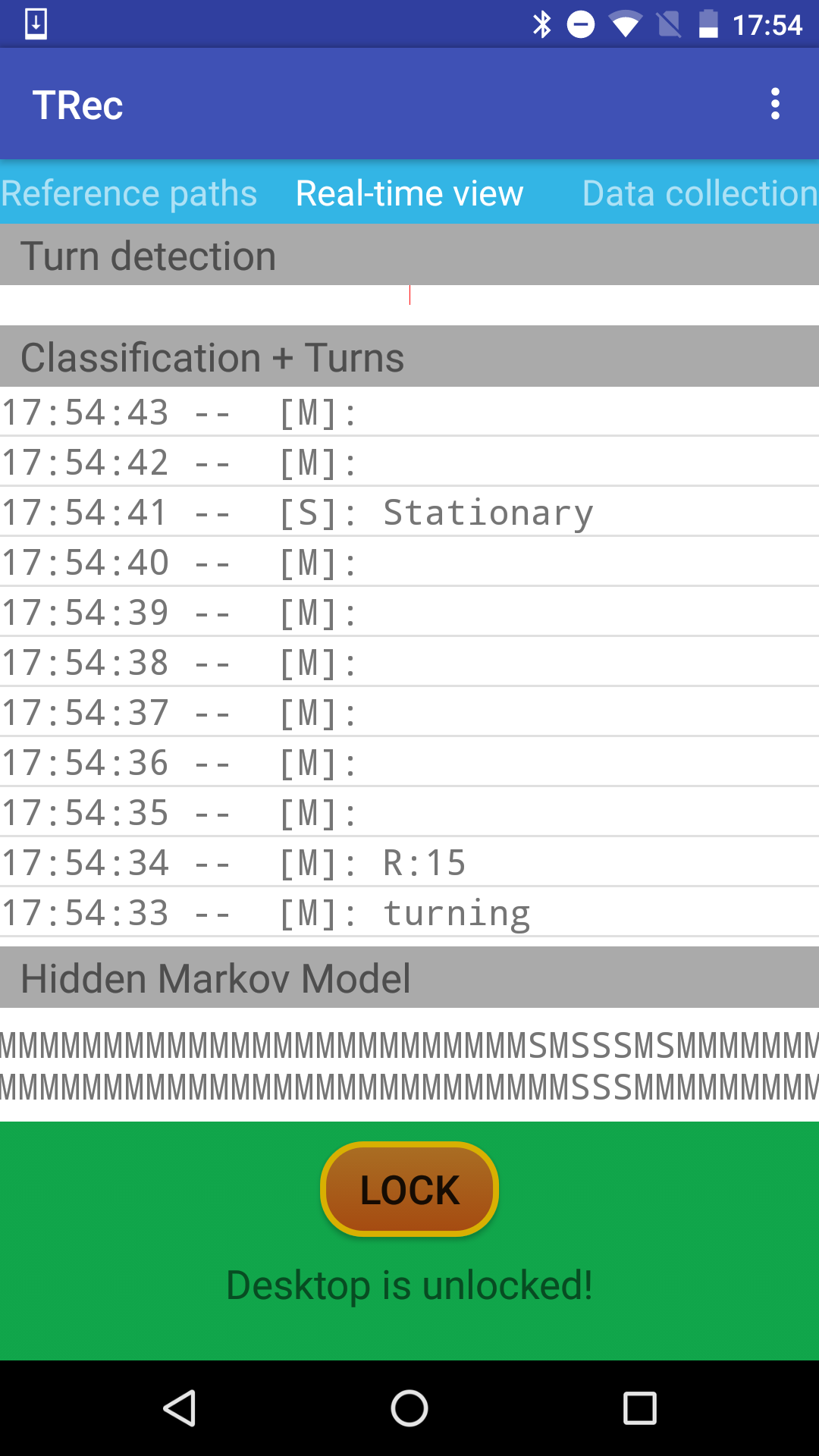
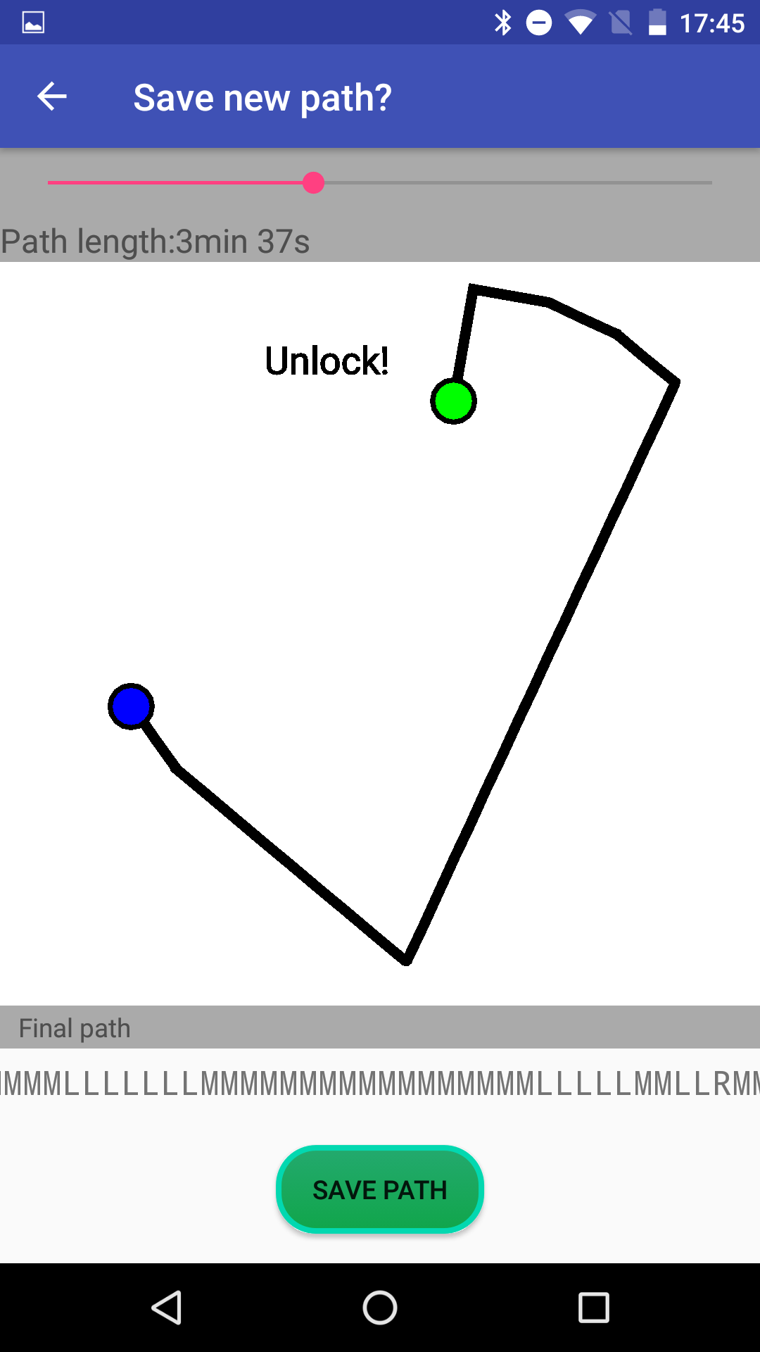
Figure 8: STASH classifies movement at one second intervals. Left: Users can quickly lock $\mathcal{V}$ in case of false accepts. Right: Interface for saving unrecognized paths. The length of the reference path can be adjusted.

Resource requirements. STASH expects a continuous stream of raw accelerometer and gyroscope data to extract the current trajectory. It re-samples the input data to 20Hz before storing it into a memory buffer (2.3MB/h each with 32bit precision), which is a fixed circular buffer holding the past hour of measurements. The values are classified on-demand with LR and the classification results are stored into a separate circular buffer (3.6kB/h with 8 bit booleans). By calculating gravity and linear accelerometer values from raw accelerometer data, STASH’s memory buffer requirements are brought down to less than 5MB in total. We use weka [12] to model logistic regression on Android. The data is only smoothed when trajectory comparison is needed. Once triggered, comparison is done continuously at one second intervals for a set of ten attempts by default. If successful, the data is written to disk and a response is generated. Otherwise the authentication attempt is aborted, whereby explicit proximity confirmation is required.

IV-B Movement Recognition

To evaluate the accuracy of movement recognition, we collected a preliminary dataset covering different motion conditions over four hours. We applied noise-based regularization [17] to reduce potential over-learning. We then evaluated the resulting LR model using five-fold stratified cross-validation to separate training and testing data.

Out of ten features, we found that the three most significant features were the standard deviation of the 5 second and 1 second sliding window of 3D differentiated accelerometer values, and the peak-to-peak value for the 5 second sliding window of gyroscope measurements: these corresponded to 58% of the weights of the LR model. Evaluation results for LR showed a true positive rate of 98% for movement (M), and 92% for stationary (S). These probabilities are used as emission probabilities in the HMM, and we use a default value of 99% probability to switch between hidden states.

IV-C Experimental Data Acquisition

To evaluate the accuracy of STASH as a whole, we collected real-world data by repeatedly traversing a series of routes. The dataset consists of paths corresponding to 20 different, 6 to 12 minute long routes in Espoo and Oxford. In order to generalize across different devices, we gathered data from five different device models at 200Hz sampling rate. We integrated the measurement devices with bicycles to avoid uncontrolled orientation changes. Each trajectory was repeated between 7 and 11 times. Routes contain real-world obstacles, such as traffic lights, gravel, asphalt or cobblestone roads and crowds. In total, the 7.7 GB dataset consists of the equivalent of 38.6 hours of recording, collected over a total distance of 123 km.

IV-D Path Similarity Thresholds

Separability. For each of 20 unique routes $R_{k},k\in\{1,\dots,20\}$, our data contains between 7 and 11 instances $i_{R_{k}}$. In order to evaluate the within-class similarities of each route and determine if the Needleman-Wunsch measure supports consistent classification, we calculated the similarities between all pairs of instances, trimmed to a duration of 2 minutes. For each route, this results in at least 21 unique pairwise within-class, and 1595 unique pairwise between-class, similarities.

Figure 7 shows an example of within-class and between-class similarities for one such route in our dataset, with all other routes showing similar behavior. In an ideal noiseless case, all instances $i_{R}$ of a route $R$ are identical, but in real-world data, sensor noise results in a spread of similarities. While there is an overlap of within-class and between-class similarities in the score range [18,21], most within-class and between-class cases are separated, confirming that Needleman-Wunsch is indeed a good measure of similarity.

Determining the initial threshold. As described in Section III, decision thresholds that STASH uses are adapted based on the number of instances of a reference path seen so far. When only a single instance has been authorized by the user, STASH uses the initial threshold; as more instances are seen, their similarities to the reference path are used to compute a local threshold, and subsequently the mixed threshold, which is a combination of initial and local thresholds that depends increasingly less on the initial threshold as the number of seen instances of a reference path increases.

We can compute the threshold with respect to a chosen trade-off between FAR and FRR by minimizing the combined error rate $\alpha\cdot FRR+(1-\alpha)\cdot FAR$ for a specific value of the trade-off parameter $\alpha$. Figure 7 shows optimal achievable FARs and FRRs for pooled reference paths. For each value of $\alpha$, the minimum combined FAR/FRR is found by varying the decision threshold. In scenarios where the usability of the system is more important, larger $\alpha$ values should be used.

The decision threshold is naturally tied to the length $L$ of the reference path. In order for STASH to make a classification decision for a candidate path given only one instance of a reference path, we need to determine a function for the initial threshold that depends on the length of the reference path $L$. We did this by searching for the value $d_{L}$ that minimizes the combined error rate for $\alpha\in\{0.1,0.2,\dots,0.9\}$ for reference path lengths $L\in\{1,2,\dots,6\}$. This gave us 6 dependent-independent variable pairs per $\alpha$, i.e. 9 linear regressions [17]. We found that the relationship between optimal decision threshold and the length of the path is affine. Figure 7 shows that $\alpha^{*}=0.5$ is closest to equal error rate. Setting $\alpha^{*}$ to 0.5, we obtained the decision thresholds for pooled scores as:

$$\begin{split}D^{*}(L)&=9.69L-1.40\end{split}$$ (3)

These are rounded to integers such as: $D^{*}(1)=8$, $D^{*}(2)=18$ and $D^{*}(5)=47$. These particular decision thresholds serve as examples on how initial thresholds are calculated, and we use them in our STASH prototype. However, in order to give an unbiased estimate of system performance, we do not use exactly these values in the remainder of system evaluation, as this might lead to over-fitting.

TABLE I: Mean and standard deviation of FAR/FRR using only the initial decision threshold individually for 20 paths.

$L$ (min)	FAR	FRR
1.0 min	$\textbf{0.064}\pm 0.057$	$\textbf{0.137}\pm{0.143}$
2.0 min	$\textbf{0.043}\pm 0.048$	$\textbf{0.039}\pm{0.102}$
3.0 min	$\textbf{0.073}\pm 0.085$	$\textbf{0.047}\pm{0.107}$
4.0 min	$\textbf{0.072}\pm 0.074$	$\textbf{0.061}\pm{0.133}$
5.0 min	$\textbf{0.049}\pm 0.061$	$\textbf{0.057}\pm{0.103}$
6.0 min	$\textbf{0.047}\pm 0.070$	$\textbf{0.040}\pm{0.081}$

Instead, we calculate decision thresholds for each reference path separately, using the leave-one-reference-path-out method, which we use for all subsequent analysis (a training set is constructed using 19 reference paths; it is used to determine the initial threshold for the remaining reference path). Figure 7 shows the FARs and FRRs by removing one and retaining the 19 other reference paths (there are 20 lines in total). As can be seen, training set error rates below 5% are achievable for all 20 sets.

The next two sections discuss actual test error rates for specific paths that use individual and mixed thresholds, evaluated w.r.t. two different parameters: the reference path length and the number of instances of a reference path.

IV-E Impact of Reference Path Length

The mean error rates and standard deviations for our 20 reference paths using the initial threshold with varying reference path lengths are shown in Table I. FRRs are calculated over all unique combinations of dividing instances $i_{R}$ of routes $R$ into reference path instances (training) and candidate paths (testing). FARs are calculated by treating all other instances $i_{\bar{R}}$ of routes $\bar{R}$ as candidate paths. We know the temporal length of the reference path and require the same length for each candidate path. Both FAR and FRR drop when increasing the length of the path from one to two minute, and reach lowest mean FAR and FRR on 2 and 6 min long reference paths. Initially, the mean FAR is between 4.3% and 7.3% and FRR between 3.9% and 6.1% for reference paths longer than two minutes. However, the variation in FRRs is high between different reference paths. We see a clear drop at 2 min, but FARs/FRRs for individual paths do not change significantly beyond $L=2$ min (Wilcoxon signed rank test). We thus use $L=2$ min for the rest of the analysis in this paper.

IV-F Using Multiple Reference Path Instances

Multiple instances of a reference path can be used to increase security and usability of the system. This is done by selecting a good representative for the reference path among the seen instances (the instance at the cluster center - the medoid) and by adopting a mixed threshold using equations 1 and 2 (combination of $d_{i}$ and $d_{l}$). The local decision threshold is calculated with the same scheme as the initial decision threshold, by setting $\alpha=0.5$. If there are multiple solutions that provide the same minimum error rate, we use the decision threshold that is center most among these for a maximum margin. The difference to the initial threshold derivation is that we generate paths to estimate the distribution of between-class similarities using a Markov chain [17]. This is done to prevent over-learning by only using collected, real world paths.

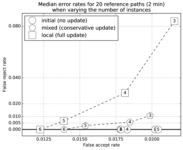
Figure 9: Increasing the number of instances of reference paths leads to a median decrease in FAR and FRR. The extent of this effect varies depending on the used threshold derivation algorithm. Coordinates describe median (FAR, FRR), numbers describe number of instances used.

To evaluate the effects of using the medoid and Equation 2 to calculate the confidence factor $\lambda$ we plotted the median FARs and FRRs (per reference path), by varying the number of instances and the decision threshold calculation scheme. It is easier to investigate trends with the median, since it is a robust estimator that tolerates outliers better than the mean. Figure 9 shows the median FARs and FRRs for the initial, local and mixed thresholds using 2 min reference paths. These represent doing no update, doing a full update or a conservative update to the decision threshold, respectively. At each update, the pairwise similarities are calculated between the instances, and the instance with the largest summed similarity to the other instances is selected as the medoid. The medoid is used for calculating the similarity to each new candidate path. The benefit in using the medoid to represent the reference path is that only one similarity score needs to be calculated, and that the score is calculated on the most representative instance. In Figure 9, circles represent the continued usage of the initial threshold. The median FRR is zero, but the FAR does not improve with more instances, because the FAR depends on the decision threshold, not on the reference path representative. Using the initial threshold is equivalent to a constant confidence factor $\lambda=0$, no trust in $d_{l}$.

The squares represents the effect of using only the local threshold. While FARs are at a similar level as the initial threshold, median FRRs are significantly worse. With five or more instances, median FARs drop to a lower level than with initial thresholds. Using only the local threshold is equivalent to a constant confidence factor $\lambda=1$ (full trust in $d_{l}$).

Mixed thresholds are derived from initial and local threshold values using equations 1 and 2, and are shown with pentagons. The mixed thresholds retain the good FRR of initial thresholds when few reference path instances are seen, and achieve improved performance similar to local thresholds when more instances have been observed. Using the confidence factor in conjunction with medoids to calculate decision thresholds is empirically shown to increase performance on two-minute paths, dropping the median FAR from $2.0\%\to 1.5\%$ when increasing the number of instances from 1 to 5, while the median FRR increases from $0.0\%\to 0.3\%$. Simultaneously, the mean FAR drops from $4.3\%\to 3.4\%$ and mean FRR drops from $3.8\%\to 2.8\%$. To further validate our results, we analyze the results of STASH when five instances are used with mixed thresholds.

Table II shows the resulting mean FARs and FRRs for different reference path lengths. Mean FARs are in the range of 2.3% to 5.0% and mean FRRs are in the range of 1.8% to 3.1% for reference paths longer than 2 min. Both FAR and FRR are smaller for these paths, and the spreads in FRRs are significantly lower than in Table I. We find again that FARs/FRRs for individual paths do not change significantly by considering reference paths beyond 2 min (Wilcoxon signed rank test).

Figure 10 shows box-and-whiskers plots [17] for FARs and FRRs for our 20 reference paths, evaluated over different lengths, once five instances have been observed by STASH. The outer lines of the boxes denote the 75th and 25th percentiles, while the line in the boxes denotes the median. The whiskers denote the range, i.e. maximum and minimum values. Note that on average, FARs and FRRs are lower than the mean values reported in Table II.

TABLE II: Mean and standard deviation of FAR/FRR using five instances and mixed decision thresholds for 20 paths.

$L$ (min)	FAR	FRR
1.0 min	$\textbf{0.141}\pm 0.135$	$\textbf{0.046}\pm{0.054}$
2.0 min	$\textbf{0.034}\pm 0.049$	$\textbf{0.028}\pm{0.042}$
3.0 min	$\textbf{0.023}\pm 0.028$	$\textbf{0.018}\pm{0.031}$
4.0 min	$\textbf{0.050}\pm 0.078$	$\textbf{0.031}\pm{0.050}$
5.0 min	$\textbf{0.042}\pm 0.058$	$\textbf{0.017}\pm{0.032}$
6.0 min	$\textbf{0.030}\pm 0.050$	$\textbf{0.015}\pm{0.032}$

For reference paths longer than 2 min, median FARs are below 3% and FRRs below 0.5%.

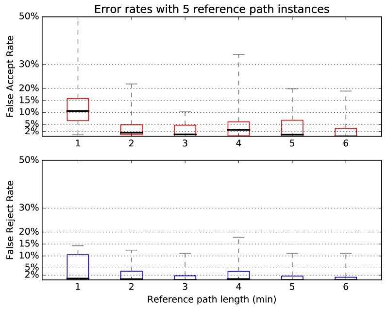
Figure 10: Mixed decision thresholds. Box-and-whiskers plot over FARs and FRRs of different temporal lengths when STASH has seen five instances of a reference path. On average FARs are below 3% and FRRs are below 0.5% when $L\geq 2min$.

Our implementation of STASH uses mixed thresholds so that its performance improves with time.

IV-G Energy Consumption

To evaluate requirement R3, we created a controlled experiment to measure the energy consumption of STASH. We obtained 3-hour consumption reports on three different devices, ten times each. A control group had no STASH installed, and did not have WiFi nor mobile connectivity.

Case 1. We model a scenario where an office employee periodically moves away from her workplace and returns back, triggering an access control decision. Movement initiates data collection at full sampling rate. Upon approaching the premise, and thus $\mathcal{V}$, path recognition is triggered and runs 60 times. Table III reports the net contribution of STASH, compared to the control group. The increase in energy consumption varies between devices. On average we recorded a drain of $0.56\%$ (of total battery capacity) per hour.

TABLE III: Net increases in hourly battery consumption rates (percentage of total capacity) and milliampere (case 1).

Device	$\%/h$	$mA$
Nexus 5	$0.41\pm 0.23$	($9.32\pm 5.22$)
Nexus 5X	$0.63\pm 0.33$	($17.13\pm 8.92$)
Samsung S6	$0.61\pm 0.24$	($15.45\pm 6.44$)

Case 2. We observed that the largest contributor to battery usage was the wakelock that ensured sensor measurements were processed quickly and not lost due to an overflowing sensor buffer. Therefore, we recorded the energy usage with wakelock acquired for three hours. This represents the worst case scenario. The hourly net battery drains for our devices are shown in Table IV. The mean increase in battery usage varies across devices, with an overall average of $1.9\%$ per hour. We believe that the drain increase in Nexus 5X and Samsung S6 is a result of these devices using different power states efficiently, causing the consumption in the control group to be lower.

TABLE IV: Net increases in hourly battery consumption rates (percentage of total capacity) and milliampere (case 2).

Device	$\%/h$	$mA$
Nexus 5	$0.87\pm 0.28$	($20.11\pm 6.40$)
Nexus 5X	$2.31\pm 0.24$	($62.28\pm 6.60$)
Samsung S6	$2.55\pm 0.17$	($65.14\pm 4.33$)

Case 3. Energy consumption of smart phone models can vary significantly for different settings and sensors. On average users recharge their batteries within an hour of depletion [29]. A study [21] found the average battery life to be nine hours (11% consumption rate) under favorable circumstances. In a setting where $\mathcal{U}$ commutes for one hour and does office work for eight hours, we estimate (using data from Tables III and IV) the additional battery drain due to STASH to be between 4% and 7%, depending on the phone model. These correspond to a decrease of approximately 20-40 minutes for a device with a battery life of nine hours. For comparison, the loss in battery life when moving from an area with average WiFi to bad coverage was estimated to be 6.29% [21].

V Security Analysis

STASH prevents relay attacks by having $\mathcal{P}$ verify its proximity to $\mathcal{V}$ through prover-side trajectory comparison: if $\mathcal{P}$’s current trajectory (candidate path) matches the authorized approach trajectory (reference path) to $\mathcal{V}$, $\mathcal{P}$ locally decides to participate in the authentication protocol with $\mathcal{V}$.

To evaluate the security guarantees of STASH, we analyze our dataset (Section IV) corresponding to a total of 123 km equivalent to 38.6 hours of movement. We used false accept rate of trajectory comparison as the measure for security. We showed that, on average, an adversary has a less then 5% chance even when STASH has only observed one instance of a reference path (Table I). This drops steadily as more instances are collected so that we can report a rate below 3.5% in Table II on average and 1.5% in median (Figure 9) after 5 path instances.

For a successful relay attack (a) $\mathcal{A}$ is required to follow $\mathcal{U}$ in close proximity and (b) $\mathcal{P}$ has to be in motion in order to produce a path recording. In a typical attack scenario, a thief tries to gain access through $\mathcal{V}$ to steal a keyless-entry car while $\mathcal{U}$ and $\mathcal{P}$ are stationary which leads to a failing proximity verification and thus $\mathcal{P}$ denying access to the authentication credentials. In this case STASH successfully improves security by completely preventing the relay attack.

The security of the trajectory leading to $\mathcal{V}$ is inversely proportional to the likelihood that there exists another route (not terminating in $\mathcal{V}$) that $\mathcal{A}$ could use to mount a relay attack if $\mathcal{U}$ happens to traverse it. The measure for security however depends on the geographic neighborhood: for instance, a trajectory with many turns can be considered to be more complex than a straight-line in most cities but in an old town that has few straight roads, such a trajectory may be uniquer. We can incorporate such uniqueness assessment of a reference path into STASH by analyzing a city’s road data to find paths that are similar to a given reference path and hence vulnerable to relay attacks. This is equivalent to the likelihood of the user unintentionally authenticating to $\mathcal{V}$ while she is traversing some other route not leading to $\mathcal{V}$. This estimate can be used as a security level indicator.

VI Discussion and Future Work

Why transparent authentication. When trajectory comparison fails, STASH will prompt the user for explicit proximity confirmation as to whether the current candidate path should be included in the set of authorized reference paths for a given verifier. The popularity of keyless entry as a premium feature across different car manufacturers suggest that consumers are willing to pay for the convenience of transparent authentication. Google’s Trust API (Project Abacus) [14] underscores TA as a trend. STASH’s contribution is to retain the convenience promised by transparent authentication while significantly enhancing resilience against relay attacks.

Verification of return paths. By relying on reference path instances gathered over time, STASH is currently limited to scenarios with stationary verifiers. But since STASH represents trajectories as sequences of primitives it is possible to compare a reference path that starts from the location of the verifier to a candidate path that ends at the verifier by reversing the reference path. This allows transparent authentication even for mobile verifiers: e.g., when a user parks his car at a new place and goes to a mall and returns to the car via the same route. Our evaluation showed promising results, and we leave its comprehensive analysis for future work.

Prover orientation changes. If $\mathcal{P}$ is a portable device like a smart phone, fast changes in $\mathcal{P}$’s orientation (e.g. taking the phone out of the pocket) affect turn detection reliability. In our evaluation, we avoided this by integrating $\mathcal{P}$ with a vehicle, we chose a bike for our experiments.

Additional sequence primitives. While this paper focuses only on using low-cost internal sensors, STASH can be extended to use additional primitives besides movement, left and right turn. If the requirement to use only internal sensors is relaxed, the system could start detecting presence of specific wireless networks or indoor short-range beacons; if the user is indeed taking the same path as was the case when the corresponding reference path was recorded, then the same events should be detected at specific locations. Such detected presences can easily be represented by additional symbols and seamlessly integrated into the current implementation of STASH. Additionally, while we currently focus only on a single movement modality, STASH can be augmented with a transport mode detection scheme [13] that would add further entropy and hence uniqueness to generated paths. As such, a path that includes walking, then taking a bus, and then walking would be more specific than if all movement intervals are represented with the same symbol.

VII Related Work

Trajectory recognition. Trajectory recognition estimates the location of a user and can be used to enable additional convenience functions but also to subvert a user’s privacy. The following techniques do not rely on GPS location information but use a different way to obtain location ground truth, e.g. a street map or the timetable of public transportation. After a correlation between mobile measurements and this information the system estimate the user’s location.

Gao et al. [8] propose an approach using vehicular speed and the start location to estimate final destination and path of a car. By matching these segments to map data they achieved an accuracy of 500 meters for 24% of traces in the New Jersey and 26% of traces in the Seattle area. Further, Watanabe et al. [30] identify a user’s train trips based on inertial measurements. First, the user’s activity is classified into inside a vehicle, walking and remaining stationary. Afterwards, the transition times between the different modes are used to correlate them with timetables. Each train trip is weighted according to its popularity to reduce the number of candidates. Their results show that location detection along train networks is feasible. The work by Nawaz and Mascolo [19] explores the significant transport routes of a user based on gyroscope data. According to their hypothesis, a route exposes a certain signature based on angular momentum. They apply dynamic time warping to account for differences in routes due to traffic conditions. Our system in contrast ignores stationary phases which makes time warping unnecessary. As shown by Narain et al. [18], it is possible to infer routes taken by a user solely based on permission free on-board sensors, e.g. gyroscope. Hence, to protect a user’s privacy our approach processes the information locally without the need of a remote service.

Co-presence verification. The co-location of devices is an important countermeasure against impersonation and relay attacks. In some cases it is also used as a second factor for authentication. Although GPS could be used to assert co-location in theory, these signals are not authenticated and thus not trustworthy [26]. A range of alternatives based on context comparison has recently emerged.

Halevi et al. [11] propose co-presence detection based on comparing audio and light. A merchant terminal and mobile phone probe their environments to compare them to assert co-location. They evaluate both modalities separately, and achieve a FAR of 6.5% and a 5% FRR for light while reporting a FAR and FRR of 0% for audio.

A similar approach to mitigate relay attacks is explored by Shrestha et al. [22] and Truong et al. [27]. They use natural environment properties as well as digital signals. Truong et al. [27] identify WiFi as the dominating feature with a FAR of 2% and a FRR of 1%. In their approach, Shrestha et al. conclude that a modality fusion reduces the FRR of up to 24% and FAR of up to 33% of an individual features to 3% and 6% respectively. However, in follow-up work they were able to increase the FAR from 3% to 66% by manipulating a single modality [23]. Hence, increasing the number of modalities does not necessarily strengthen security as it depends on the weights machine learning models assign to them. A thorough analysis of these algorithms is required to give sophisticated security guarantees. Karapanos et al. [16] use the audio fingerprint of a location as a second factor for authentication. Their threat model assumes a remote attacker who obtained the user’s credentials.

VIII Conclusion

We proposed, implemented and evaluated STASH, a novel approach to prevent relay attacks in transparent authentication schemes. As STASH is entirely realized on the prover device it allows easy integration into existing systems while preserving the user’s privacy at the same time. The performance of our approach and the negligible resource requirements make it a valuable extension of current TA schemes.

Algorithm 1 Turn detection with angular data.

Heading angle $\alpha(t_{0})=0$

repeat

     Update heading angle $\alpha(t_{i})$

     Update rolling standard deviation for last 2 seconds

     Update time when turn begins ($t_{begin}$) and ends ($t_{end}$)

     if turn ends then

         $d=\alpha(t_{end})-\alpha(t_{begin})$

         $n=|round(d/15^{\circ})|$

         if $d>0$ then

              add $n$ symbols $R$

         else[$d<0$]

              add $n$ symbols $L$               

until app closed

Algorithm 1 shows pseudocode for our turn detection algorithm. Gyroscope and accelerometer signals are re-sampled to 20Hz in STASH. Axis-specific gyroscope noise is set to zero during stationary time ($std<0.01$). Gyroscope events are realigned to the earth’s frame by projecting along the gravity direction. The heading angle is acquired by integration (initial angle zero). Turns (yaw angle differences) are acquired continuously with Algorithm 1.

Trajectories are defined a sequences of $M$ (movement) and $L/R$ (left/right) primitives. Parameters used in STASH are shown in Table V. Movement is classified with a logistic regression function every second. A hidden Markov model smooths the classified result into the sequence of most likely events. The sequence of movement and turn events are combined with turns taking precedence. Table V summarizes parameters used in STASH. Trajectory comparison is done using the Needleman-Wunsch (NW) algorithm.

TABLE V: Parameter used in STASH.

Parameter	value
Movement event time	$5$ seconds
$M$-event TPR	98 %
$S$-event TPR	92 %
HMM prior $p(M\rightarrow M)$	99 %
HMM prior $p(S\rightarrow S)$	99 %
Movement classification frequency	$1$ second
HMM Viterbi smoothing	at arrival to $\mathcal{V}$
Turn event granularity	$15^{\circ}$
Gyroscope flatten std thr.	$0.01^{\circ}$
Turn detection std thr.	$3^{\circ}$
Turn fine-tune std thr.	$1^{\circ}$
Needleman-Wunsch match	$+1$
Needleman-Wu. mismatch	$-2$
Needleman-Wunsch gap	$-1$

Table VI shows the initial decision thresholds in NW obtained by minimizing the error rate $\alpha\cdot FRR+(1-\alpha)\cdot FAR$. A candidate path is accepted if its similarity to a reference path is higher than the decision threshold. The values are calculated for the pooled thresholds (see Section IV-D).

TABLE VI: Decision thresholds for Needleman-Wunsch algorithm, w.r.t. trajectory lengths in minutes. The r value for the OLS fit is shown in parentheses.

$\alpha$	$D(L)$
$0.1$	$10.171L+1.400$ ($r=0.998$)
$0.2$	$10.314L-0.600$ ($r=0.999$)
$0.3$	$10.143L-1.000$ ($r=0.999$)
$0.4$	$9.543L-0.067$ ($r=0.998$)
$0.5$	$9.686L-1.400$ ($r=0.998$)
$0.6$	$9.914L-2.533$ ($r=0.998$)
$0.7$	$9.771L-3.533$ ($r=0.996$)
$0.8$	$8.600L-1.600$ ($r=0.993$)
$0.9$	$7.914L-2.200$ ($r=0.989$)

References

- [1] Android. Keeping the device awake, 2016. https://developer.android.com/training/scheduling/wakelock.html.
- [2] J. Bonneau, C. Herley, P. C. van Oorschot, and F. Stajano. The quest to replace passwords: A framework for comparative evaluation of web authentication schemes. In IEEE Symposium on Security and Privacy, SP 2012, 21-23 May 2012, San Francisco, California, USA, pages 553–567. IEEE Computer Society, 2012.
- [3] J. Bonneau, C. Herley, P. C. van Oorschot, and F. Stajano. Passwords and the evolution of imperfect authentication. Commun. ACM, 58(7):78–87, 2015.
- [4] S. Brands and D. Chaum. Distance-Bounding Protocols. In Advances in Cryptology — EUROCRYPT ’93, pages 344–359. Springer Berlin Heidelberg, Berlin, Heidelberg, 1993.
- [5] M. D. Corner and B. D. Noble. Zero-interaction authentication. In Proceedings of the 8th annual international conference on Mobile computing and networking - MobiCom ’02, page 1, New York, New York, USA, sep 2002. ACM Press.
- [6] D. Dolev and A. C. Yao. On the security of public key protocols. Information Theory, IEEE Transactions on, 29(2):198–208, 1983.
- [7] R. Durbin, S. R. Eddy, A. Krogh, and G. Mitchison. Biological sequence analysis: probabilistic models of proteins and nucleic acids. Cambridge university press, 1998.
- [8] B. Firner, S. Sugrim, Y. Yang, and J. Lindqvist. Elastic pathing: Your speed is enough to track you. arXiv preprint arXiv:1401.0052, pages 975–986, 2013.
- [9] A. Francillon, B. Danev, and S. Capkun. Relay Attacks on Passive Keyless Entry and Start Systems in Modern Cars. Network and Distributed System Security Symposium, pages 431–439, 2011.
- [10] L. Francis, G. Hancke, K. Mayes, and K. Markantonakis. Practical relay attack on contactless transactions by using NFC mobile phones. In Cryptology and Information Security Series, volume 8, pages 21–32, 2012.
- [11] T. Halevi, D. Ma, N. Saxena, and T. Xiang. Secure Proximity Detection for NFC Devices Based on Ambient Sensor Data. pages 379–396. Springer Berlin Heidelberg, 2012.
- [12] M. Hall, E. Frank, G. Holmes, B. Pfahringer, P. Reutemann, and I. H. Witten. The weka data mining software: an update. ACM SIGKDD explorations newsletter, 11(1):10–18, 2009.
- [13] S. Hemminki, P. Nurmi, and S. Tarkoma. Accelerometer-based transportation mode detection on smartphones. In Proceedings of the 11th ACM Conference on Embedded Networked Sensor Systems, page 13. ACM, 2013.
- [14] A. Hern. Google aims to kill passwords by the end of this year — Technology — The Guardian, 2016.
- [15] A. R. Jimenez, F. Seco, C. Prieto, and J. Guevara. A comparison of pedestrian dead-reckoning algorithms using a low-cost mems imu. In Intelligent Signal Processing, 2009. WISP 2009. IEEE International Symposium on, pages 37–42. IEEE, 2009.
- [16] N. Karapanos, C. Marforio, C. Soriente, and S. Capkun. Sound-Proof: Usable Two-Factor Authentication Based on Ambient Sound. In 24th USENIX Security Symposium (USENIX Security 15), pages 483–498, 2015.
- [17] K. P. Murphy. Machine learning: a probabilistic perspective. MIT press, 2012.
- [18] S. Narain, T. D. Vo-Huu, K. Block, and G. Noubir. Inferring user routes and locations using zero-permission mobile sensors. 2016.
- [19] S. Nawaz and C. Mascolo. Mining users’ significant driving routes with low-power sensors. In Proceedings of the 12th ACM Conference on Embedded Network Sensor Systems, pages 236–250. ACM, 2014.
- [20] V. M. Patel, R. Chellappa, D. Chandra, and B. Barbello. Continuous User Authentication on Mobile Devices: Recent progress and remaining challenges. IEEE Signal Processing Magazine, 33(4):49–61, jul 2016.
- [21] E. Peltonen, E. Lagerspetz, P. Nurmi, and S. Tarkoma. Energy modeling of system settings: A crowdsourced approach. In Pervasive Computing and Communications (PerCom), 2015 IEEE International Conference on, pages 37–45. IEEE, 2015.
- [22] B. Shrestha, N. Saxena, H. T. T. Truong, and N. Asokan. Drone to the Rescue: Relay-Resilient Authentication using Ambient Multi-sensing. pages 349–364. Springer Berlin Heidelberg, 2014.
- [23] B. Shrestha, N. Saxena, H. T. T. Truong, and N. Asokan. Contextual Proximity Detection in the Face of Context-Manipulating Adversaries. Nov 2015. arXiv report /1511.00905 http://arxiv.org/abs/1511.00905.
- [24] SourceForge. BlueProximity. https://sourceforge.net/projects/blueproxi-mity/.
- [25] A. Tefas, C. Kotropoulos, and L. Pitas. Using Support Vector Machines to enhance the performance of elastic graph matching for frontal face authentication. IEEE Transactions on Pattern Analysis and Machine Intelligence, 23(7):735–746, 2001.
- [26] N. O. Tippenhauer, C. Pöpper, K. B. Rasmussen, and S. Capkun. On the requirements for successful GPS spoofing attacks. ACM conference on Computer and communications security, CCS, page 75, 2011.
- [27] H. T. T. Truong, X. Gao, B. Shrestha, N. Saxena, N. Asokan, and P. Nurmi. Using contextual co-presence to strengthen Zero-Interaction Authentication: Design, integration and usability. Pervasive and Mobile Computing, 16:187–204, 2015.
- [28] H. T. T. Truong, B. Shrestha, N. Saxena, N. Asokan, and P. Nurmi. Comparing and fusing different sensor modalities for relay attack resistance in Zero-Interaction Authentication. In 2014 IEEE International Conference on Pervasive Computing and Communications (PerCom), pages 163–171. IEEE, mar 2014.
- [29] D. T. Wagner, A. Rice, and A. R. Beresford. Device analyzer: Understanding smartphone usage. In International Conference on Mobile and Ubiquitous Systems: Computing, Networking, and Services, pages 195–208. Springer, 2013.
- [30] T. Watanabe, M. Akiyama, and T. Mori. RouteDetector: Sensor-based Positioning System That Exploits Spatio-Temporal Regularity of Human Mobility. 2015.
- [31] G. Xiao, M. Milanova, and M. Xie. Secure behavioral biometric authentication with leap motion. In 2016 4th International Symposium on Digital Forensic and Security (ISDFS), pages 112–118. IEEE, apr 2016.