The Stochastic Topic Block Model for the Clustering of Vertices in Networks with Textual Edges

Abstract

Due to the significant increase of communications between individuals via social media (Facebook, Twitter, Linkedin) or electronic formats (email, web, e-publication) in the past two decades, network analysis has become a unavoidable discipline. Many random graph models have been proposed to extract information from networks based on person-to-person links only, without taking into account information on the contents. This paper introduces the stochastic topic block model (STBM), a probabilistic model for networks with textual edges. We address here the problem of discovering meaningful clusters of vertices that are coherent from both the network interactions and the text contents. A classification variational expectation-maximization (C-VEM) algorithm is proposed to perform inference. Simulated data sets are considered in order to assess the proposed approach and to highlight its main features. Finally, we demonstrate the effectiveness of our methodology on two real-word data sets: a directed communication network and a undirected co-authorship network.

1 Introduction

The significant and recent increase of interactions between individuals via social media or through electronic communications enables to observe frequently networks with textual edges. It is obviously of strong interest to be able to model and cluster the vertices of those networks using information on both the network structure and the text contents. Techniques able to provide such a clustering would allow a deeper understanding of the studied networks. As a motivating example, Figure 1 shows a network made of three “communities” of vertices where one of the communities can in fact be split into two separate groups based on the topics of communication between nodes of these groups (see legend of Figure 1 for details). Despite the important efforts in both network analysis and text analytics, only a few works have focused on the joint modeling of network vertices and textual edges.

Figure 1: A sample network made of 3 “communities” where one of the communities is made of two topic-specific groups. The left panel only shows the observed (binary) edges in the network. The center panel shows the network with only the partition of edges into 3 topics (edge colors indicate the majority topics of texts). The right panel shows the network with the clustering of its nodes (vertex colors indicate the groups) and the majority topic of the edges. The latter visualization allows to see the topic-conditional structure of one of the three communities.

1.1 Statistical models for network analysis

On the one hand, there is a long history of research in the statistical analysis of networks, which has received strong interest in the last decade. In particular, statistical methods have imposed theirselves as efficient and flexible techniques for network clustering. Most of those methods look for specific structures, so called communities, which exhibit a transitivity property such that nodes of the same community are more likely to be connected (Hofman and Wiggins, 2008). Popular approaches for community discovering, though asymptotically biased (Bickel and Chen, 2009), are based on the modularity score given by Girvan and Newman (2002). Alternative clustering methods usually rely on the latent position cluster model (LPCM) of Handcock et al. (2007), or the stochastic block model (SBM) (Wang and Wong, 1987; Nowicki and Snijders, 2001). The LPCM model, which extends the work of Hoff et al. (2002), assumes that the links between the vertices depend on their positions in a social latent space and allows the simultaneous visualization and clustering of a network.

The SBM model is a flexible random graph model which is based on a probabilistic generalization of the method applied by White et al. (1976) on Sampson’s famous monastery (Fienberg and Wasserman, 1981). It assumes that each vertex belongs to a latent group, and that the probability of connection between a pair of vertices depends exclusively on their group. Because no specific assumption is made on the connection probabilities, various types of structures of vertices can be taken into account. At this point, it is important to notice that, in network clustering, two types of clusters are usually considered: communities (vertices within a community are more likely to connect than vertices of different communities) and stars or disassortative clusters (the vertices of a cluster highly connect to vertices of another). In this context, SBM is particularly useful in practice since it has the ability to characterize both types of clusters.

While SBM was originally developed to analyze mainly binary networks, many extensions have been proposed since to deal for instance with valued edges (Mariadassou et al., 2010), categorical edges (Jernite et al., 2014) or to take into account prior information (Zanghi et al., 2010; Matias and Robin, 2014). Note that other extensions of SBM have focused on looking for overlapping clusters (Airoldi et al., 2008; Latouche et al., 2011) or on the modeling of dynamic networks (Yang et al., 2011; Xu and Hero III, 2013; Bouveyron et al., 2016; Matias and Miele, 2016).

The inference of SBM-like models is usually done using variational expectation maximization (VEM) (Daudin et al., 2008), variational Bayes EM (VBEM) (Latouche et al., 2012), or Gibbs sampling (Nowicki and Snijders, 2001). Moreover, we emphasize that various strategies have been derived to estimates the number of corresponding clusters using model selection criteria (Daudin et al., 2008; Latouche et al., 2012), allocation sampler (Mc Daid et al., 2013), greedy search (Côme and Latouche, 2015), or non parametric schemes (Kemp et al., 2006). We refer to (Salter-Townshend et al., 2012) for a overview of statistical models for network analysis.

1.2 Statistical models for text analytics

On the other hand, the statistical modeling of texts appeared at the end of the last century with an early model described by Papadimitriou et al. (1998) for latent semantic indexing (LSI) (Deerwester et al., 1990). LSI is known in particular for allowing to recover linguistic notions such as synonymy and polysemy from “term frequency - inverse document frequency” (tf-idf) data. Hofmann (1999) proposed an alternative model for LSI, called probabilistic latent semantic analysis (pLSI), which models each word within a document using a mixture model. In pLSI, each mixture component is modeled by a multinomial random variable and the latent groups can be viewed as “topics”. Thus, each word is generated from a single topic and different words in a document can be generated from different topics. However, pLSI has no model at the document level and may suffer from overfitting. Notice that pLSI can also be viewed has an extension of the mixture of unigrams, proposed by Nigam et al. (2000).

The model which finally concentrates most desired features was proposed by Blei et al. (2003) and is called latent Dirichlet allocation (LDA). The LDA model has rapidly become a standard tool in statistical text analytics and is even used in different scientific fields such has image analysis (Lazebnik et al., 2006) or transportation research (Côme et al., 2014) for instance. The idea of LDA is that documents are represented as random mixtures over latent topics, where each topic is characterized by a distribution over words. LDA is therefore similar to pLSI except that the topic distribution in LDA has a Dirichlet distribution. Several inference procedures have been proposed in the literature ranging from VEM (Blei et al., 2003) to collapsed VBEM (Teh et al., 2006).

Note that a limitation of LDA would be the inability to take into account possible topic correlations. This is due to the use of the Dirichlet distribution to model the variability among the topic proportions. To overcome this limitation, the correlated topic model (CTM) was also developed by Blei and Lafferty (2006). Similarly, the relational topic model (RTM) (Chang and Blei, 2009) models the links between documents as binary random variables conditioned on their contents, but ignoring the community ties between the authors of these documents. Notice that the “itopic” model (Sun et al., 2009) extends RTM to weighted networks. The reader may refer to Blei (2012) for an overview on probabilistic topic models.

1.3 Statistical models for the joint analysis of texts and networks

Finally, a few recent works have focused on the joint modeling of texts and networks. Those works are mainly motivated by the will of analyzing social networks, such as Twitter or Facebook, or electronic communication networks. Some of them are partially based on LDA: the author-topic (AT) (Steyvers et al., 2004; Rosen-Zvi et al., 2004) and the author-recipient-topic (ART) (McCallum et al., 2005) models. The AT model extends LDA to include authorship information whereas the ART model includes authorships and information about the recipients. Though potentially powerful, these models do not take into account the network structure (communities, stars, …) while the concept of community is very important in the context of social networks, in the sense that a community is a group of users sharing similar interests.

Among the most advanced models for the joint analysis of texts and networks, the first models which explicitly take into account both text contents and network structure are the community-user-topic (CUT) models proposed by (Zhou et al., 2006). Two models are proposed: CUT1 and CUT2, which differ on the way they construct the communities. Indeed, CUT1 determines the communities only based on the network structure whereas CUT2 model the communities based on the content information solely. The CUT models therefore deal each with only a part of the problem we are interested in. It is also worth noticing that the authors of these models rely for inference on Gibbs sampling which may prohibit their use on large networks.

A second attempt was made by Pathak et al. (2008) who extended the ART model by introducing the community-author-recipient-topic (CART) model. The CART model adds to the ART model that authors and recipients belong to latent communities and allows CART to recover groups of nodes that are homogenous both regarding the network structure and the message contents. Notice that CART allows the nodes to be part of multiple communities and each couple of actors to have a specific topic. Thus, though extremely flexible, CART is also a highly parametrized model. In addition, the recommended inference procedure based on Gibbs sampling may also prohibit its application to large networks.

More recently, the topic-link LDA (Liu et al., 2009) also performs topic modeling and author community discovery in a unified framework. As its name suggests, topic-link LDA extends LDA with a community layer where the link between two documents (and consequently its authors) depends on both topic proportions and author latent features through a logistic transformation. However, whereas CART focuses only on directed networks, topic-link LDA is only able to deal with undirected networks. On the positive side, the authors derive a variational EM algorithm for inference, allowing topic-link LDA to eventually be applied to large networks.

Finally, a family of 4 topic-user-community models (TUCM) were proposed by Sachan et al. (2012). The TUCM models are designed such that they can find topic-meaningful communities in networks with different types of edges. This in particular relevant in social networks such as Twitter where different types of interactions (followers, tweet, re-tweet, …) exist. Another specificity of the TUCM models is that they allow both multiple community and topic memberships. Inference is also done here through Gibbs sampling, implying a possible scale limitation.

1.4 Contributions and organization of the paper

We propose here a new generative model for the clustering of networks with textual edges, such as communication or co-authorship networks. Conversely to existing works which have either too simple or highly-parametrized models for the network structure, our model relies for the network modeling on the SBM model which offers a sufficient flexibility with a reasonable complexity. This model is one of the few able to recover different topological structures such as communities, stars or disassortative clusters (see Latouche et al., 2012, for instance). Regarding the topic modeling, our approach is based on the LDA model, in which the topics are conditioned on the latent groups. Thus, the proposed modeling will be able to exhibit node partitions that are meaningful both regarding the network structure and the topics, with a model of limited complexity, highly interpretable, and for both directed and undirected networks. In addition, the proposed inference procedure – a classification-VEM algorithm – allows the use of our model on large-scale networks.

The proposed model, named stochastic topic block model (STBM), is introduced in Section 2. The model inference is discussed in Section 3 as well as model selection. Section 4 is devoted to numerical experiments highlighting the main features of the proposed approach and proving the validity of the inference procedure. Two applications to real-world networks (the Enron email and the Nips co-authorship networks) are presented in Section 5. Section 6 finally provides some concluding remarks.

2 The model

This section presents the notations used in the paper and introduces the STBM model. The joint distributions of the model to create edges and the corresponding documents are also given.

2.1 Context and notations

A directed network with $M$ vertices, described by its $M\times M$ adjacency matrix $A$, is considered. Thus, $A_{ij}=1$ if there is an edge from vertex $i$ to vertex $j$, $0$ otherwise. The network is assumed not to have any self-loop and therefore $A_{ii}=0$ for all $i$. If an edge from $i$ to $j$ is present, then it is characterized by a set of $D_{ij}$ documents, denoted $W_{ij}=(W_{ij}^{d})_{d}$. Each document $W_{ij}^{d}$ is made of a collection of $N_{ij}^{d}$ words $W_{ij}^{d}=(W_{ij}^{dn})_{n}$. In the directed scenario considered, $W_{ij}$ can model for instance a set of emails or text messages sent from actor $i$ to actor $j$. Note that all the methodology proposed in this paper easily extends to undirected networks. In such a case, $A_{ij}=A_{ji}$ and $W_{ij}^{d}=W_{ji}^{d}$ for all $i$ and $j$. The set $W_{ij}^{d}$ of documents can then model for example books or scientific papers written by both $i$ and $j$. In the following, we denote $W=(W_{ij})_{ij}$ the set of all documents exchanged, for all the edges present in the network.

Our goal is to cluster the vertices into $Q$ latent groups sharing homogeneous connection profiles, i.e. find an estimate of the set $Y=(Y_{1},\dots,Y_{M})$ of latent variables $Y_{i}$ such that $Y_{iq}=1$ if vertex $i$ belongs to cluster $q$, and $0$ otherwise. Although in some cases, discrete or continuous edges are taken into account, the literature on networks focuses on modeling the presence of edges as binary variables. The clustering task then consists in building groups of vertices having similar trends to connect to others. In this paper, the connection profiles are both characterized by the presence of edges and the documents between pairs of vertices. Therefore, we aim at uncovering clusters by integrating these two sources of information. Two nodes in the same cluster should have the same trend to connect to others, and when connected, the documents they are involved in should be made of words related to similar topics.

2.2 Modeling the presence of edges

In order to model the presence of edges between pairs of vertices, a stochastic block model (Wang and Wong, 1987; Nowicki and Snijders, 2001) is considered. Thus, the vertices are assumed to be spread into $Q$ latent clusters such that $Y_{iq}=1$ if vertex $i$ belongs to cluster $q$, and $0$ otherwise. In practice, the binary vector $Y_{i}$ is assumed to be drawn from a multinomial distribution

$$Y_{i}\sim\mathcal{M}\left(1,\rho=(\rho_{1},\dots,\rho_{Q})\right),$$

where $\rho$ denotes the vector of class proportions. By construction, $\sum_{q=1}^{Q}\rho_{q}=1$ and $\sum_{q=1}^{Q}Y_{iq}=1,\forall i$.

An edge from $i$ to $j$ is then sampled from a Bernoulli distribution, depending on their respective clusters

$$A_{ij}|Y_{iq}Y_{jr}=1\sim\mathcal{B}(\pi_{qr}).$$ (1)

In words, if $i$ is in cluster $q$ and $j$ in $r$, then $A_{ij}$ is $1$ with probability $\pi_{qr}$. In the following, we denote $\pi$ the $Q\times Q$ matrix of connection probabilities. Note that in the undirected case, $\pi$ is symmetric.

All vectors $Y_{i}$ are sampled independently, and given $Y=(Y_{1},\dots,Y_{M})$, all edges in $A$ are assumed to be independent. This leads to the following joint distribution

$$p(A,Y|\rho,\pi)=p(A|Y,\pi)p(Y|\rho),$$

where

$$p(A|Y,\pi) =\prod_{i\neq j}^{M}p(A_{ij}|Y_{i},Y_{j},\pi)$$

$$=\prod_{i\neq j}^{M}\prod_{q,l}^{Q}p(A_{ij}|\pi_{qr})^{Y_{iq}Y_{jr}},$$

and

$$p(Y|\rho) =\prod_{i=1}^{M}p(Y_{i}|\rho)$$

$$=\prod_{i=1}^{M}\prod_{q=1}^{Q}\rho_{q}^{Y_{iq}}.$$

2.3 Modeling the construction of documents

As mentioned previously, if an edge is present from vertex $i$ to vertex $j$, then a set of documents $W_{ij}=(W_{ij}^{d})_{d}$, characterizing the oriented pair $(i,j)$, is assumed to be given. Thus, in a generative perspective, the edges in $A$ are first sampled using previous section. Given $A$, the documents in $W=(W_{ij})_{ij}$ are then constructed. The generative process we consider to build documents is strongly related to the latent Dirichlet allocation (LDA) model of Blei et al. (2003). The link between STBM and LDA is made clear in the following section. The STBM model relies on two concepts at the core of the SBM and LDA models respectively. On the one hand, a generalization of the SBM model would assume that any kind of relationships between two vertices can be explained by their latent clusters only. In the LDA model on the other hand, the main assumption is that words in documents are drawn from a mixture distribution over topics, each document $d$ having its own vector of topic proportions $\theta_{d}$. The STBM model combines these two concepts to introduce a new generative procedure for documents in networks.

Each pair of clusters $(q,r)$ of vertices is first associated to a vector of topic proportions $\theta_{qr}=(\theta_{qrk})_{k}$ sampled independently from a Dirichlet distribution

$$\theta_{qr}\sim\mathrm{Dir}\left(\alpha=(\alpha_{1},\dots,\alpha_{K})\right),$$

such that $\sum_{k=1}^{K}\theta_{qrk}=1,\forall(q,r)$. We denote $\theta=(\theta_{qr})_{qr}$ and $\alpha=(\alpha_{1},\dots,\alpha_{K})$ the parameter vector controlling the Dirichlet distribution. Note that in all our experiments we set each component of $\alpha$ to $1$ in order to obtain a uniform distribution. Since $\alpha$ is fixed, it does not appear in the conditional distributions provided in the following. The $n$th word $W_{ij}^{dn}$ of documents $d$ in $W_{ij}$ is then associated to a latent topic vector $Z_{ij}^{dn}$ assumed to be drawn from a multinomial distribution, depending on the latent vectors $Y_{i}$ and $Y_{j}$

$$Z_{ij}^{dn}|\left\{Y_{iq}Y_{jr}A_{ij}=1,\theta\right\}\sim\mathcal{M}\left(1,\theta_{qr}=(\theta_{qr1},\dots,\theta_{qrK})\right).$$ (2)

Note that $\sum_{k=1}^{K}Z_{ij}^{dnk}=1,\forall(i,j,d),A_{ij}=1$. Equations (1) and (2) are related: they both involve the construction of random variables depending on the cluster assignment of vertices $i$ and $j$. Thus, if an edge is present ($A_{ij}=1$) and if $i$ is in cluster $q$ and $j$ in $r$, then the word $W_{ij}^{dn}$ is in topic $k$ ($Z_{ij}^{dnk}=1$) with probability $\theta_{qrk}$.

Then, given $Z_{ij}^{dn}$, the word $W_{ij}^{dn}$ is assumed to be drawn from a multinomial distribution

$$W_{ij}^{dn}|Z_{ij}^{dnk}=1\sim\mathcal{M}\left(1,\beta_{k}=(\beta_{k1},\dots,\beta_{kV})\right),$$ (3)

where $V$ is the number of (different) words in the vocabulary considered and $\sum_{v=1}^{V}\beta_{kv}=1,\forall k$ as well as $\sum_{v=1}^{V}W_{ij}^{dnv}=1,\forall(i,j,d,n)$. Therefore, if $W_{ij}^{dn}$ is from topic $k$, then it is associated to word $v$ of the vocabulary ($W_{ij}^{dnv}=1$) with probability $\beta_{kv}$. Equations (2) and (3) lead to the following mixture model for words over topics

$$W_{ij}^{dn}|\left\{Y_{iq}Y_{jr}A_{ij}=1,\theta\right\}\sim\sum_{k=1}^{K}\theta_{qrk}\mathcal{M}\left(1,\beta_{k}\right),$$

where the $K\times V$ matrix $\beta=(\beta_{kv})_{kv}$ of probabilities does not depend on the cluster assignments. Note that words of different documents $d$ and $d^{{}^{\prime}}$ in $W_{ij}$ have the same mixture distribution which only depends on the respective clusters of $i$ and $j$. We also point out that words of the vocabulary appear in any document $d$ of $W_{ij}$ with probabilities

$$\mathbb{P}(W_{ij}^{dnv}=1|Y_{iq}Y_{jr}A_{ij}=1,\theta)=\sum_{k=1}^{K}\theta_{qrk}\beta_{kv}.$$

Because pairs $(q,r)$ of clusters can have different vectors of topics proportions $\theta_{qr}$, the documents they are associated with can have different mixture distribution of words over topics. For instance, most words exchanged from vertices of cluster $q$ to vertices of cluster $r$ can be related to mathematics while vertices from $q^{\prime}$ can discuss with vertices of $r^{\prime}$ with words related to cinema and in some cases to sport.

All the latent variables $Z_{ij}^{dn}$ are assumed to be sampled independently and, given the latent variables, the words $W_{ij}^{dn}$ are assumed to be independent. Denoting $Z=(Z_{ij}^{dn})_{ijdn}$, this leads to the following joint distribution

$$p(W,Z,\theta|A,Y,\beta)=p(W|A,Z,\beta)p(Z|A,Y,\theta)p(\theta),$$

where

$$p(W|A,Z,\beta) =\prod_{i\neq j}^{M}\left\{\prod_{d=1}^{D_{ij}}\prod_{n=1}^{N_{ij}^{d}}p(W_{ij}^{dn}|Z_{ij}^{dn},\beta)\right\}^{A_{ij}}$$

$$=\prod_{i\neq j}^{M}\left\{\prod_{d=1}^{D_{ij}}\prod_{n=1}^{N_{ij}^{d}}\prod_{k=1}^{K}p(W_{ij}^{dn}|\beta_{k})^{Z_{ij}^{dnk}}\right\}^{A_{ij}},$$

and

$$p(Z|A,Y,\theta) =\prod_{i\neq j}^{M}\left\{\prod_{d=1}^{D_{ij}}\prod_{n=1}^{N_{ij}^{d}}p(Z_{ij}^{dn}|Y_{i},Y_{j},\theta)\right\}^{A_{ij}}$$

$$=\prod_{i\neq j}^{M}\left\{\prod_{d=1}^{D_{ij}}\prod_{n=1}^{N_{ij}^{d}}\prod_{q,r}^{Q}p(Z_{ij}^{dn}|\theta_{qr})^{Y_{iq}Y_{jr}}\right\}^{A_{ij}},$$

as well as

$$p(\theta)=\prod_{q,r}^{Q}\mathrm{Dir}(\theta_{qr};\alpha).$$

2.4 Link with LDA and SBM

Figure 2: Graphical representation of the stochastic topic block model.

The full joint distribution of the STBM model is given by

$$p(A,W,Y,Z,\theta|\rho,\pi,\beta)=p(W,Z,\theta|A,Y,\beta)p(A,Y|\rho,\pi),$$ (4)

and the corresponding graphical model is provided in Figure 2. Thus, all the documents in $W$ are involved in the full joint distribution through $p(W,Z,\theta|A,Y,\beta)$. Now, let us assume that $Y$ is available. It then possible to reorganize the documents in $W$ such that $W=(\tilde{W}_{qr})_{qr}$ where $\tilde{W}_{qr}=\left\{W_{ij}^{d},\forall(d,i,j),Y_{iq}Y_{jr}A_{ij}=1\right\}$ is the set of all documents exchanged from any vertex $i$ in cluster $q$ to any vertex $j$ in cluster $r$. As mentioned in the previous section, each word $W_{ij}^{dn}$ has a mixture distribution over topics which only depends on the clusters of $i$ and $j$. Because all words in $\tilde{W}_{qr}$ are associated with the same pair $(q,r)$ of clusters, they share the same mixture distribution. Removing temporarily the knowledge of $(q,r$), i.e. simply seeing $\tilde{W}_{qr}$ as a document $d$, the sampling scheme described previously then corresponds to the one of a LDA model with $D=Q^{2}$ independent documents $\tilde{W}_{qr}$, each document having its own vector $\theta_{qr}$ of topic proportions. The model is then characterized by the matrix $\beta$ of probabilities. Note that contrary to the original LDA model (Blei et al., 2003), the Dirichlet distributions considered for the $\theta_{qr}$ depend on a fixed vector $\alpha$.

As mentioned in Section 2.2, the second part of Equation (4) involves the sampling of the clusters and the construction of binary variables describing the presence of edges between pairs of vertices. Interestingly, it corresponds exactly to the complete data likelihood of the SBM model, as considered in Zanghi et al. (2008) for instance. Such a likelihood term only involves the model parameters $\rho$ and $\pi$.

3 Inference

We aim at maximizing the complete data log-likelihood

$$\log p(A,W,Y|\rho,\pi,\beta)=\log\sum_{Z}\int_{\theta}p(A,W,Y,Z,\theta|\rho,\pi,\beta)d\theta,$$ (5)

with respect to the model parameters $(\rho,\pi,\beta)$ and the set $Y=(Y_{1},\dots,Y_{M})$ of cluster membership vectors. Note that $Y$ is not seen here as a set of latent variables over which the log-likelihood should be integrated out, as in standard expectation maximization (EM) (Dempster et al., 1977) or variational EM algorithms (Hathaway, 1986). Moreover, the goal is not to provide any approximate posterior distribution of $Y$ given the data and model parameters. Conversely, $Y$ is seen here as a set of (binary) vectors for which we aim at providing estimates. This choice is motivated by the key property of the STBM model, i.e. for a given $Y$, the full joint distribution factorizes into a LDA like term and SBM like term. In particular, given $Y$, words in $W$ can be seen as being drawn from a LDA model with $D=Q^{2}$ documents (see Section 2.4), for which fast optimization tools have been derived, as pointed out in the introduction. Note that the choice of optimizing a complete data log-likelihood with respect to the set of cluster membership vectors has been considered in the literature, for simple mixture model such as Gaussian mixture models, but also for the SBM model (Zanghi et al., 2008). The corresponding algorithm, so called classification EM (CEM) (Celeux and Govaert, 1991) alternates between the estimation of $Y$ and the estimation of the model parameters.

As mentioned previously, we introduce our methodology in the directed case. However, we emphasize that the STBM package for R we developed, implements the inference strategy for both directed and undirected networks.

3.1 Variational decomposition

Unfortunately, in our case, Equation (5) is not tractable. Moreover the posterior distribution $p(Z,\theta|A,W,Y,\rho,\pi,\beta)$ does not have any analytical form. Therefore, following the work of Blei et al. (2003) on the LDA model, we propose to rely on a variational decomposition. In the case of the STBM model, it leads to

$$\log p(A,W,Y|\rho,\pi,\beta)=\mathcal{L}\left(R(\cdot);Y,\rho,\pi,\beta\right)+\mathrm{KL}\left(R(\cdot)\parallel p(\cdot|A,W,Y,\rho,\pi,\beta\right)),$$

where

$$\mathcal{L}\left(R(\cdot);Y,\rho,\pi,\beta\right)=\sum_{Z}\int_{\theta}R(Z,\theta)\log\frac{p(A,W,Y,Z,\theta|\rho,\pi,\beta)}{R(Z,\theta)}d\theta,$$ (6)

and $\mathrm{KL}$ denotes the Kullback-Leibler divergence between the true and approximate posterior distribution $R(\cdot)$ of $(Z,\theta)$, given the data and model parameters

$$\mathrm{KL}\left(R(\cdot)\parallel p(\cdot|A,W,Y,\rho,\pi,\beta\right))=-\sum_{Z}\int_{\theta}R(Z,\theta)\log\frac{p(Z,\theta|A,W,Y,\rho,\pi,\beta)}{R(Z,\theta)}d\theta.$$

Since $\log p(A,W,Y|\rho,\pi,\beta)$ does not depend on the distribution $R(Z,\theta)$, maximizing the lower bound $\mathcal{L}$ with respect to $R(Z,\theta)$ induces a minimization of the KL divergence. As in Blei et al. (2003), we assume that $R(Z,\theta)$ can be factorized over the latent variables in $\theta$ and $Z$. In our case, this translates into

$$R(Z,\theta)=R(Z)R(\theta)=R(\theta)\prod_{i\neq j,A_{ij}=1}^{M}\prod_{d=1}^{D_{ij}}\prod_{n=1}^{N_{ij}^{d}}R(Z_{ij}^{dn}).$$

3.2 Model decomposition

As pointed out in Section 2.4, the set of latent variables in $Y$ allows the decomposition of the full joint distribution in two terms, from the sampling of $Y$ and $A$ to the construction of documents given $A$ and $Y$. When deriving the lower bound (6), this property leads to

$$\mathcal{L}\left(R(\cdot);Y,\rho,\pi,\beta\right)=\tilde{\mathcal{L}}\left(R(\cdot);Y,\beta\right)+\log p(A,Y|\rho,\pi),$$

where

$$\tilde{\mathcal{L}}\left(R(\cdot);Y,\beta\right)=\sum_{Z}\int_{\theta}R(Z,\theta)\log\frac{p(W,Z,\theta|A,Y,\beta)}{R(Z,\theta)}d\theta,$$ (7)

and $\log p(A,Y|\rho,\pi)$ is the complete data log-likelihood of the SBM model. The parameter $\beta$ and the distribution $R(Z,\theta)$ are only involved in the lower bound $\tilde{\mathcal{L}}$ while $\rho$ and $\pi$ only appear in $\log p(A,Y|\rho,\pi)$. Therefore, given $Y$, these two terms can be maximized independently. Moreover, given $Y$, $\tilde{\mathcal{L}}$ is the lower bound for the LDA model, as proposed by Blei et al. (2003), after building the set $W=(\tilde{W}_{qr})_{qr}$ of $D=Q^{2}$ documents, as described in Section 2.4. In the next section, we derive a VEM algorithm to maximize $\tilde{\mathcal{L}}$ with respect $\beta$ and $R(Z,\theta)$, which essentially corresponds to the VEM algorithm of Blei et al. (2003). Then, $\log p(A,Y|\rho,\pi)$ is maximized with respect to $\rho$ and $\pi$ to provide estimates. Finally, $\mathcal{L}\left(R(\cdot);Y,\rho,\pi,\beta\right)$ is maximized with respect to $Y$, which is the only term involved in both $\tilde{\mathcal{L}}$ and the SBM complete data log-likelihood. Because the methodology we propose requires a variational EM approach as well as a classification step, to provide estimates of $Y$, we call the corresponding strategy a classification VEM (C-VEM) algorithm.

3.3 Optimization

In this section, we derive the optimization steps of the C-VEM algorithm we propose, which aims at maximizing the lower bound $\mathcal{L}$. The algorithm alternates between the optimization of $R(Z,\theta)$, $Y$ and $(\rho,\pi,\beta)$ until convergence of the lower bound.

Estimation of $R(Z,\theta)$

The following propositions give the update formulae of the E step of the VEM algorithm applied on Equation (7).

Proposition 1

(Proof in Appendix  A.1) The VEM update step for each distribution $R(Z_{ij}^{dn})$ is given by

$$R(Z_{ij}^{dn})=\mathcal{M}\left(Z_{ij}^{dn};1,\phi_{ij}^{dn}=(\phi_{ij}^{dn1},\dots,\phi_{ij}^{dnK})\right),$$

where

$$\phi_{ij}^{dnk}\propto\left(\prod_{v=1}^{V}\beta_{kv}^{W_{ij}^{dnv}}\right)\prod_{q,r}^{Q}\exp\Big{(}\psi(\gamma_{qrk}-\psi(\sum_{l=1}^{K}\gamma_{qrl})\Big{)}^{Y_{iq}Y_{jr}},\forall(d,n,k).$$

$\phi_{ij}^{dnk}$ is the (approximate) posterior distribution of words $W_{ij}^{dn}$ being in topic $k$.

Proposition 2

(Proof in Appendix  A.2) The VEM update step for distribution $R(\theta)$ is given by

$$R(\theta)=\prod_{q,r}^{Q}\mathrm{Dir}(\theta_{qr};\gamma_{qr}=(\gamma_{qr1},\dots,\gamma_{qrK})),$$

where

$$\gamma_{qrk}=\alpha_{k}+\sum_{i\neq j}^{M}A_{ij}Y_{iq}Y_{jr}\sum_{d=1}^{N_{ij}^{d}}\sum_{n=1}^{N_{ij}^{dn}}\phi_{ij}^{dnk},\forall(q,r,k).$$

Estimation of the model parameters

Maximizing the lower bound $\mathcal{L}$ in Equation (7) is used to provide estimates of the model parameters $(\rho,\pi,\beta)$. We recall that $\beta$ is only involved in $\tilde{\mathcal{L}}$ while $(\rho,\pi)$ only appear in the SBM complete data log-likelihood. The derivation of $\tilde{\mathcal{L}}$ is given in Appendix A.3.

Proposition 3

(Proofs in Appendices  A.4, A.5, A.6) The estimates of $\beta$, $\rho$, and $\pi$, are given by

$$\beta_{kv}\propto\sum_{i\neq j}^{M}A_{ij}\sum_{d=1}^{D_{ij}}\sum_{n=1}^{N_{ij}^{dn}}\phi_{ij}^{dnk}W_{ij}^{dnv},\forall(k,v),$$

$$\rho_{q}\propto\sum_{i=1}^{M}Y_{iq},\forall q,$$

$$\pi_{qr}=\frac{\sum_{i\neq j}^{M}\sum_{q,r}^{Q}Y_{iq}Y_{jr}A_{ij}}{\sum_{i\neq j}^{M}\sum_{q,r}^{Q}Y_{iq}Y_{jr}},\forall(q,r).$$

Estimation of $Y$

At this step, the model parameters $(\rho,\pi,\beta)$ along with the distribution $R(Z,\theta)$ are held fixed. Therefore, the lower bound $\mathcal{L}$ in (7) only involves the set $Y$ of cluster membership vectors. Looking for the optimal solution $Y$ maximizing this bound is not feasible since it involves testing the $Q^{M}$ possible cluster assignments. However, heuristics are available to provide local maxima for this combinatorial problem. These so called greedy methods have been used for instance to look for communities in networks by Newman (2004); Blondel et al. (2008) but also for the SBM model (Côme and Latouche, 2015). They are sometimes referred to as on line clustering methods (Zanghi et al., 2008).

The algorithm cycles randomly through the vertices. At each step, a single vertex is considered and all membership vectors $Y_{j}$ are held fixed, except $Y_{i}$. If $i$ is currently in cluster $q$, then the method looks for every possible label swap, i.e. removing $i$ from cluster $q$ and assigning it to a cluster $r\neq q$. The corresponding change in $\mathcal{L}$ is then computed. If no label swap induces an increase in $\mathcal{L}$, then $Y_{i}$ remains unchanged. Otherwise, the label swap that yields the maximal increase is applied, and $Y_{i}$ is changed accordingly.

3.4 Initialization strategy and model selection

The C-VEM introduced in the previous section allows the estimation of $R(Z,\theta)$, $Y$, as well as $(\rho,\pi,\beta$), for a fixed number $Q$ of clusters and a fixed number $K$ of topics. As any EM-like algorithms, the C-VEM method depends on the initialization and is only guaranteed to converge to a local optimum (Bilmes, 1998). Strategies to tackle this issue include simulated annealing and the use of multiple initializations (Biernacki et al., 2003). In this work, we choose the latter option. Our C-VEM algorithm is run for several initializations of a k-means like algorithm on a distance matrix between the vertices obtained as follows.

1. The VEM algorithm (Blei et al., 2003) for LDA is applied on the aggregation of all documents exchanged from vertex $i$ to vertex $j$, for each pair $(i,j)$ of vertices, in order to characterize a type of interaction from $i$ to $j$. Thus, a $M\times M$ matrix $X$ is first built such that $X_{ij}=k$ if $k$ is the majority topic used by $i$ when discussing with $j$.

2. The distance $M\times M$ matrix $\Delta$ is then computed as follows

   $$\Delta(i,j)=\sum_{h=1}^{N}\delta(X_{ih}\neq X_{jh})A_{ih}A_{jh}+\sum_{h=1}^{N}\delta(X_{hi}\neq X_{hj})A_{hi}A_{hj}.$$ (8)

   The first term looks at all possible edges from $i$ and $j$ towards a third vertex $h$. If both $i$ and $j$ are connected to $h$, i.e. $A_{ih}A_{jh}=1$, the edge types $X_{ih}$ and $X_{jh}$ are compared. By symmetry, the second term looks at all possible edges from a vertex $h$ to both $i$ as well as $j$, and compare their types. Thus, the distance computes the number of discordances in the way both $i$ and $j$ connect to other vertices or vertices connect to them.

Regarding model selection, since a model based approach is proposed here, two STBM models will be seen as different if they have different values of $Q$ and/or $K$. Therefore, the task of estimating $Q$ and $K$ can be viewed as a model selection problem. Many model selection criteria have been proposed in the literature, such as the Akaike information criterion (Akaike, 1973) (AIC) and the Bayesian information criterion (Schwarz, 1978) (BIC). In this paper, because the optimization procedure considered involves the optimization of the binary matrix $Y$, we rely on a ICL-like criterion. This criterion was originally proposed by Biernacki et al. (2000) for Gaussian mixture models. In the STBM context, it aims at approximating the integrated complete data log-likelihood $\log p(A,W,Y)$.

Proposition 4

(Proof in Appendix  A.7) A $ICL$ criterion for the STBM model can be obtained

$$ICL_{STBM}=\tilde{\mathcal{L}}(R(\cdot);Y,\beta)-\frac{K(V-1)}{2}\log Q^{2}+\max_{\rho,\pi}\log p(A,Y|\rho,\pi,Q)-\frac{Q^{2}}{2}\log M(M-1)-\frac{Q-1}{2}\log M$$

Notice that this result relies on two Laplace approximations, a variational estimation, as well as Stirling formula. It is also worth noticing that this criterion involves two parts, as shown in the appendix: a BIC like term associated to a LDA model (see Than and Ho, 2012, for instance) with $Q^{2}$ documents and the ICL criterion for the SBM model, as introduced by Daudin et al. (2008).

4 Numerical experiments

This section aims at highlighting the main features of the proposed approach on synthetic data and at proving the validity of the inference algorithm presented in the previous section. Model selection is also considered to validate the criterion choice. Numerical comparisons with state-of-the-art methods conclude this section.

4.1 Experimental setup

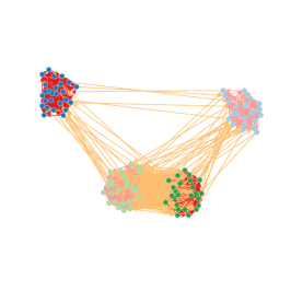
Scenario A	Scenario B	Scenario C

Figure 3: Networks sampled according to the three simulation scenarios A, B and C. See text for details.

Scenario	A	B	C
M (nb of nodes)	100
K (topics)	4	3	3
Q (groups)	3	2	4
$\rho$ (group prop.)	$(1/Q,...,1/Q)$
$\pi$ (connection prob.)	$\begin{cases}\pi_{qq}=&0.25\\ \pi_{qr,\,r\neq q}=&0.01\end{cases}$	$\pi_{qr,\,\forall q,r}=0.25$	$\begin{cases}\pi_{qq}=&0.25\\ \pi_{qr,\,r\neq q}=&0.01\end{cases}$
$\theta$ (prop. of topics)	$\begin{cases}\theta_{111}=\theta_{222}=&1\\ \theta_{333}=&1\\ \theta_{qr4,\,r\neq q}=&1\\ \textnormal{otherwise}&0\end{cases}$	$\begin{cases}\theta_{111}=\theta_{222}=&1\\ \theta_{qr3,\,r\neq q}=&1\\ \textnormal{otherwise}&0\end{cases}$	$\begin{cases}\theta_{111}=\theta_{331}=&1\\ \theta_{222}=\theta_{442}=&1\\ \theta_{qr3,\,r\neq q}=&1\\ \textnormal{otherwise}&0\end{cases}$

Table 1: Parameter values for the three simulation scenarios (see text for details).

First, regarding the parametrization of our approach, we chose $\alpha_{k}=1,\forall k$ which induces a uniform distribution over the topic proportions $\theta_{qr}$.

Second, regarding the simulation setup and in order to illustrate the interest of the proposed methodology, three different simulation setups will be used in this section. To simplify the characterization and facilitate the reproducibility of the experiments, we designed three different scenarios. They are as follows:

• scenario A consists in networks with $Q=3$ groups, corresponding to clear communities, where persons within a group talk preferentially about a unique topic and use a different topic when talking with persons of other groups. Thus, those networks contain $K=4$ topics.

• scenario B consists in networks with a unique community where the $Q=2$ groups are only differentiated by the way they discuss within and between groups. Persons within groups 1 and 2 talk preferentially about topics 1 and 2 respectively. A third topic is used for the communications between persons of different groups.

• scenario C, finally, consists in networks with $Q=4$ groups which use $K=3$ topics to communicate. Among the $4$ groups, two groups correspond to clear communities where persons talk preferentially about a unique topic within the communities. The two other groups correspond to a single community and are only discriminated by the topic used in the communications. People from group 3 use topic 1 and the topic 2 is used in group 4. The third topic is used for communications between groups.

For all scenarios, the simulated messages are sampled from four texts from BBC news: one text is about the birth of Princess Charlotte, the second one is about black holes in astrophysics, the third one is focused on UK politics and the last one is about cancer diseases in medicine. All messages are made of 150 words. Table 1 provides the parameter values for the three simulation scenarios. Figure 3 shows simulated networks according to the three simulation scenarios. It is worth noticing that all simulation scenarios have been designed such that they do not to strictly follow the STBM model and therefore they do not favor the model we propose in comparisons.

4.2 Introductory example

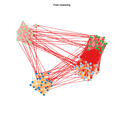
Figure 4: Clustering result for the introductory example (scenario C). See text for details.

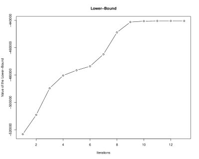
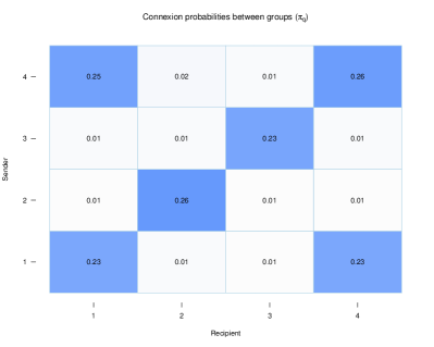
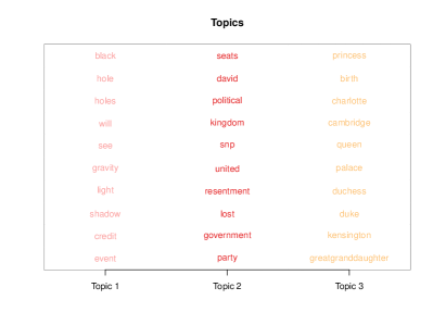
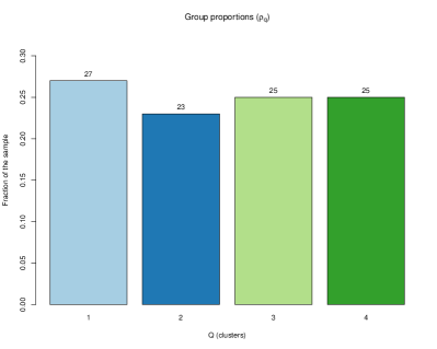
Figure 5: Clustering result for the introductory example (scenario C). See text for details.

As an introductory example, we consider a network of $M=100$ nodes sampled according to scenario C ($3$ communities, $Q=4$ groups and $K=3$ topics). This scenario corresponds to a situation where both network structure and topic information are needed to correctly recover the data structure. Indeed, groups 3 and 4 form a single community when looking at the network structure and it is necessary to look at the way they communicate to discriminate the two groups.

The C-VEM algorithm for STBM was run on the network with the actual number of groups and topics (the problem of model selection will be considered in next section). Figure 4 first shows the obtained clustering, which is here perfect both regarding the simulated node and edges partitions. More interestingly, Figure 5 allows to visualize the evolution of the lower bound $\mathcal{L}$ along the algorithm iterations (top-left panel), the estimated model parameters $\pi$ and $\rho$ (right panels), and the most frequent words in the $3$ found topics (left-bottom panel). It turns out that both the model parameters, $\pi$ and $\rho$ (see Table 1 for actual values), and the topic meanings are well recovered. STBM indeed perfectly recovers the three themes that we used for simulating the textual edges: one is a “royal baby” topic, one is a political one and the last one is focused on Physics. Notice also that this result was obtained in only a few iterations of the C-VEM algorithm, that we proposed for inferring STBM models.

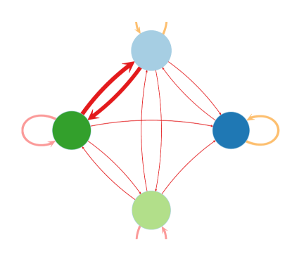
Figure 6: Introductory example: summary of connexion probabilities between groups ($\pi$, edge widths), group proportions ($\rho$, node sizes) and most probable topics for group interactions (edge colors).

A useful and compact view of both parameters $\pi$ and $\rho$, and of the most probable topics for group interactions can be offered by Figure 6. Here, edge widths correspond to connexion probabilities between groups ($\pi$), the node sizes are proportional to group proportions ($\rho$) and edge colors indicate the majority topics for group interactions. It is important to notice that, even though only the most probable topic is displayed here, each textual edge may use different topics.

4.3 Model selection

Scenario A ($Q=3$, $K=4$)
$K$\$Q$	1	2	3	4	5	6
1	0	0	0	0	0	0
2	12	0	0	0	0	0
3	0	0	0	0	0	0
4	0	0	82	2	0	2
5	0	0	2	0	0	0
6	0	0	0	0	0	0

Scenario B ($Q=2$, $K=3$)
$K$\$Q$	1	2	3	4	5	6
1	0	0	0	0	0	0
2	12	0	0	0	0	0
3	0	88	0	0	0	0
4	0	0	0	0	0	0
5	0	0	0	0	0	0
6	0	0	0	0	0	0

Scenario C ($Q=4$, $K=3$)
$K$\$Q$	1	2	3	4	5	6
1	0	0	0	0	0	0
2	0	0	0	0	0	0
3	0	0	2	82	0	0
4	0	0	0	16	0	0
5	0	0	0	0	0	0
6	0	0	0	0	0	0

Table 2: Percentage of selections by ICL for each STBM model $(Q,K)$ on 50 simulated networks of each of three scenarios. Highlighted rows and columns correspond to the actual values for $Q$ and $K$.

This experiment focuses on the ability of the ICL criterion to select appropriate values for $Q$ and $K$. To this end, we simulated 50 networks according to each of the three scenarios and STBM was applied on those networks for values of $Q$ and $K$ ranging from $1$ to $6$. Table 2 presents the percentage of selections by ICL for each STBM model $(Q,K)$ on 50 simulated networks of each of the three scenarios.

In the three different situations, ICL succeeds most of the time in identifying the actual combination of the number of groups and topics. For scenarios A and B, when ICL does not select the correct values for $Q$ and $K$, the criterion seems to underestimate the values of $Q$ and $K$ whereas it tends to overestimate them in case of scenario C. One can also notice that wrongly selected models are usually close to the simulated one. Let us also recall that, since the data are not strictly simulated according to a STBM model, the ICL criterion does not have the model which generated the data in the set of tested models. This experiment allows to validate ICL as a model selection tool for STBM.

4.4 Benchmark study

This third experiment aims at comparing the ability of STBM to recover the network structure both in term of node partition and topics. STBM is here compared to SBM, using the mixer package (Ambroise et al., 2010), and LDA, using the topicmodels package (Grun and Hornik, 2013). Obviously, SBM and LDA will be only able to recover either the node partition or the topics. We chose here to evaluate the results by comparing the resulting node and topic partitions with the actual ones (the simulated partitions). In the clustering community, the adjusted Rand index (ARI) (Rand, 1971) serves as a widely accepted criterion for the difficult task of clustering evaluation. The ARI looks at all pairs of nodes and checks whether they are classified in the same group or not in both partitions. As a result, an ARI value close to 1 means that the partitions are similar. Notice that the actual values of $Q$ and $K$ are provided to the three algorithms.

In addition to the different simulation scenarios, we considered three different situations: the standard simulation situation as described in Table 1 (hereafter “Easy”), a simulation situation (hereafter “Hard 1”) where the communities are less differentiated ($\pi_{qq}=0.25$ and $\pi_{q\neq r}=0.2$, except for scenario B) and a situation (hereafter “Hard 2”) where $40\%$ of message words are sampled in different topics than the actual topic.

Easy		Scenario A		Scenario B		Scenario C
	Method	node ARI	edge ARI	node ARI	edge ARI	node ARI	edge ARI
	SBM	1.00$\pm$0.00	–	0.01$\pm$0.01	–	0.69$\pm$0.07	–
	LDA	–	0.97$\pm$0.06	–	1.00$\pm$0.00	–	1.00$\pm$0.00
	STBM	0.98$\pm$0.04	0.98$\pm$0.04	1.00$\pm$0.00	1.00$\pm$0.00	1.00$\pm$0.00	1.00$\pm$0.00

Hard 1		Scenario A		Scenario B		Scenario C
	Method	node ARI	edge ARI	node ARI	edge ARI	node ARI	edge ARI
	SBM	0.01$\pm$0.01	–	0.01$\pm$0.01	–	0.01$\pm$0.01	–
	LDA	–	0.90$\pm$0.17	–	1.00$\pm$0.00	–	0.99$\pm$0.01
	STBM	1.00$\pm$0.00	0.90$\pm$0.13	1.00$\pm$0.00	1.00$\pm$0.00	1.00$\pm$0.00	0.98$\pm$0.03

Hard 2		Scenario A		Scenario B		Scenario C
	Method	node ARI	edge ARI	node ARI	edge ARI	node ARI	edge ARI
	SBM	1.00$\pm$0.00	–	-0.01$\pm$0.01	–	0.65$\pm$0.05	–
	LDA	–	0.21$\pm$0.13	–	0.08$\pm$0.06	–	0.09$\pm$0.05
	STBM	0.99$\pm$0.02	0.99$\pm$0.01	0.59$\pm$0.35	0.54$\pm$0.40	0.68$\pm$0.07	0.62$\pm$0.14

Table 3: Clustering results for the SBM, LDA and STBM on 20 networks simulated according to the three scenarios. Average ARI values are reported with standard deviations for both node and edge clustering. The “Easy” situation corresponds to the simulation situation describes in Table 1. In the “Hard 1” situation, the communities are very few differentiated ($\pi_{qq}=0.25$ and $\pi_{q\neq r}=0.2$, except for scenario B). The “Hard 2” situation finally corresponds to a setup where $40\%$ of message words are sampled in different topics than the actual topic.

In the “Easy” situation, the results are coherent with our initial guess when building the simulation scenarios. Indeed, besides the fact that SBM and LDA are only able to recover one of the two partitions, scenario A is an easy situation for all methods since the clusters perfectly match the topic partition. Scenario B, which has no communities and where groups only depend on topics, is obviously a difficult situation for SBM but does not disturb LDA which perfectly recovers the topics. In scenario C, LDA still succeeds in identifying the topics whereas SBM well recognizes the two communities but fails in discriminating the two groups hidden in a single community. Here, STBM obtains in all scenarios the best performance on both nodes and edges.

The “Hard 1” situation considers the case where the communities are actually not well differentiated. Here, LDA is little affected (only in scenario A) whereas SBM is no longer able to distinguish the groups of nodes. Conversely, STBM relies on the found topics to correctly identifies the node groups and obtains, here again, excellent ARI values in all the three scenarios.

The last situation, the so-called “Hard 2” case, aims at highlighting the effect of the word sampling in the recovering of the used topics. On the one hand, SBM now achieves a satisfying classification of nodes for scenarios A and C while LDA fails in recovering the majority topic used for simulation. On those two scenarios, STBM performs well on both nodes and topics. This proves that STBM is also able to recover the topics in a noisy situation by relying on the network structure. On the other hand, scenario B presents an extremely difficult situation where topics are noised and there are no communities. Here, although both LDA and SBM fail, STBM achieves a satisfying result on both nodes and edges. This is, once again, an illustration of the fact that the joint modeling of network structure and topics allows to recover complex hidden structures in a network with textual edges.

5 Application to real-world problems

In this section, we present two applications of STBM to real-world networks: the Enron email and the Nips co-authorship networks. These two data sets have been chosen because one is a directed network of moderate size whereas the other one is undirected and of a large size.

5.1 Analysis of the Enron email network

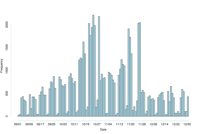
Figure 7: Frequency of messages between Enron employees between September 1st and December 31th, 2001.

We consider here a classical communication network, the Enron data set, which contains all email communications between 149 employees of the famous company from 1999 to 2002. The original data set is available at https://www.cs.cmu.edu/~./enron/. Here, we focus on the period September, 1st to December, 31th, 2001. We chose this specific time window because it is the denser period in term of sent emails and since it corresponds to a critical period for the company. Indeed, after the announcement early September 2001 that the company was “in the strongest and best shape that it has ever been in”, the Securities and Exchange Commission (SEC) opened an investigation on October, 31th for fraud and the company finally filed for bankruptcy on December, 2nd, 2001. By this time, it was the largest bankruptcy in U.S. history and resulted in more than 4,000 lost jobs. Unsurprisingly, those key dates actually correspond to breaks in the email activity of the company, as shown by Figure 7.

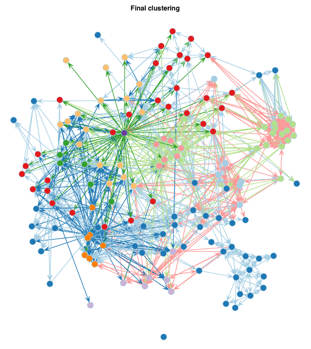
Figure 8: Clustering result with STBM on the Enron data set (Sept.-Dec. 2001).

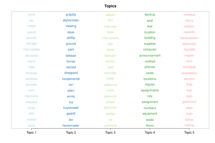
Figure 9: Most specific words for the 5 found topics with STBM on the Enron data set.

The data set considered here contains 20 940 emails sent between the $M=149$ employees. All messages sent between two individuals were coerced in a single meta-message. Thus, we end up with a data set of 1 234 directed edges between employees, each edge carrying the text of all messages between two persons.

The C-VEM algorithm we developed for STBM was run on these data for a number $Q$ of groups from $1$ to $14$ and a number $K$ of topics from $2$ to $20$. As one can see on Figure 1 of the supplementary material the model with the highest value was $(Q,K)=(10,5)$. Figure 8 shows the clustering obtained with STBM for $10$ groups of nodes and $5$ topics. As previously, edge colors refer to the majority topics for the communications between the individuals. The found topics can be easily interpreted by looking at the most specific words of each topic, displayed in Figure 9. In a few words, we can summarize the found topics as follows:

• Topic 1 seems to refer to the financial and trading activities of Enron,

• Topic 2 is concerned with Enron activities in Afghanistan (Enron and the Bush administration were suspected to work secretly with Talibans up to a few weeks before the 9/11 attacks),

• Topic 3 contains elements related to the California electricity crisis, in which Enron was involved, and which almost caused the bankruptcy of SCE-corp (Southern California Edison Corporation) early 2001,

• Topic 4 is about usual logistic issues (building equipment, computers, …),

• Topic 5 refers to technical discussions on gas deliveries (mmBTU represents 1 million of British thermal unit, which is equal to 1055 joules).

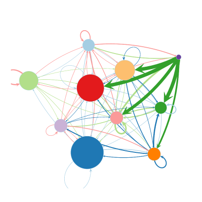
Figure 10: Enron data set: summary of connexion probabilities between groups ($\pi$, edge widths), group proportions ($\rho$, node sizes) and most probable topics for group interactions (edge colors).

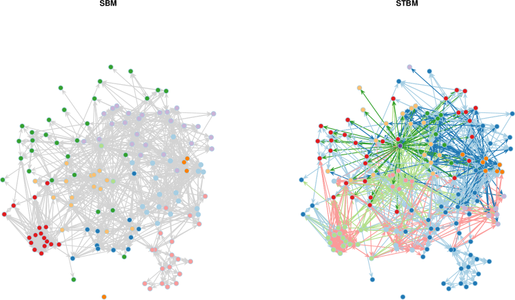
Figure 11: Clustering results with SBM (left) and STBM (right) on the Enron data set. The selected number of groups for SBM is $Q=8$ whereas STBM selects 10 groups and 5 topics.

Figure 10 presents a visual summary of connexion probabilities between groups (the estimated $\pi$ matrix) and majority topics for group interactions. A few elements deserve to be highlighted in view of this summary. First, group 10 contains a single individual who has a central place in the network and who mostly discusses about logistic issues (topic 4) with groups 4, 5, 6 and 7. Second, group 8 is made of 6 individuals who mainly communicates about Enron activities in Afghanistan (topic 2) between them and with other groups. Finally, groups 4 and 6 seem to be more focused on trading activities (topic 1) whereas groups 1, 3 and 9 are dealing with technical issues on gas deliveries (topic 5).

As a comparison, the network has also been processed with SBM, using the mixer package (Ambroise et al., 2010). The chosen number $K$ of groups by SBM was 8. Figure 11 allows to compare the partitions of nodes provided by SBM and STBM. One can observe that the two partitions differ on several points. On the one hand, some clusters found by SBM (the bottom-left one for instance) have been split by STBM since some nodes use different topics than the rest of the community. On the other hand, SBM isolates two “hubs” which seem to have similar behaviors. Conversely, STBM identifies a unique “hub” and the second node is gathered with other nodes, using similar discussion topics. STBM has therefore allowed a better and deeper understanding of the Enron network through the combination of text contents with network structure.

5.2 Analysis of the Nips co-authorship network

This second network is a co-authorship network within a scientific conference: the Neural Information Processing Systems (Nips) conference. The conference was initially mainly focused on computational neurosciences and is nowadays one of the famous conferences in statistical learning and artificial intelligence. We here consider the data between the 1988 and 2003 editions (Nips 1–17). The data set, available at http://robotics.stanford.edu/~gal/data.html, contains the abstracts of 2 484 accepted papers from 2 740 contributing authors. The vocabulary used in the paper abstracts has 14 036 words. Once the co-authorship network reconstructed, we have an undirected network between 2 740 authors with 22 640 textual edges.

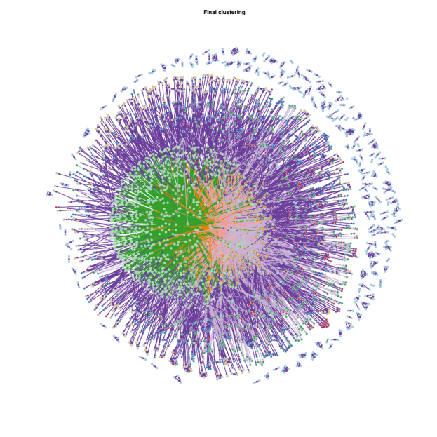
Figure 12: Clustering result with STBM on the Nips co-authorship network.

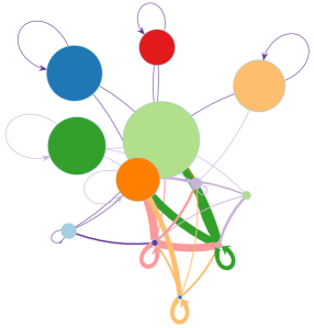
Figure 13: Nips co-authorship network: summary of connexion probabilities between groups ($\pi$, edge widths), group proportions ($\rho$, node sizes) and most probable topics for group interactions (edge colors).

We applied STBM on this large data set and the selected model by ICL was $(Q,K)=(13,7)$. The values of ICL are presented in Figure 4 of the supplementary material. Note that the values of the criterion for $K>Q$ are not indicated since we found ICL to have higher values for $K\leq Q$ on this data set. It is worth noticing that STBM chose here a limited number of topics compared to what a simple LDA analysis of the data would have provided. Indeed, STBM looks for topics which are useful for clustering the nodes. In this sense, the topics of STBM may be slightly different than those of LDA. Figure 12 shows the clustering obtained with STBM for $13$ groups of nodes and $7$ topics. Due to size and density of the network, the visualization and interpretation from this figure are actually tricky. Fortunately, the meta-view of the network shown by Figure 13 is of a greater help and allows to get a clear idea of the network organization. To this end, it is necessary to first picture out the meaning of the found topics (see Figure 14):

• Topic 1 seems to be focused on neural network theory, which was and still is a central topic in Nips,

• Topic 2 is concerned with phoneme classification or recognition,

• Topic 3 is a more general topic about statistical learning and artificial intelligence,

• Topic 4 is about Neuroscience and focuses on experimental works about the visual cortex,

• Topic 5 deals with network learning theory,

• Topic 6 is also about Neuroscience but seems to be more focused on EEG,

• Topic 7 is finally devoted to neural coding, i.e. characterizing the relationship between the stimulus and the individual responses.

In light of these interpretations, we can eventually comment some specific relationships between groups. First of all, we have an obvious community (group 1) which is disconnected with the rest of the network and which is focused on neural coding (topic 7). One can also clearly identifies, on both Figure 13 and the reorganized adjacency matrix (Figure 6 of the supplementary material) that groups 2, 5 and 10 are three “hubs” of a few individuals. Group 2 seems to mainly work on the visual cortex understanding whereas group 10 is focused on phoneme analysis. Group 5 is mainly concerned with the general neural network theory but has also collaborations in phoneme analysis. From a more general point of view, topics 6 and 7 seem to be popular themes in the network. Notice that group 3 has a specific behavior in the network since people in this cluster publish preferentially with people in other groups than together. This is the exact definition of a disassortative cluster. This appears clearly on Figure 6 of the supplementary material. It is also of interest to notice that statistical learning and artificial intelligence (which are probably now 90% of the submissions at Nips) were not yet by this time proper thematics. They were probably used more as tools in phoneme recognition studies and EEG analyses. This is confirmed by the fact that words used in topic 3 are less specific to the topic and are frequently used in other topics as well (see Figure 7 of the supplementary material).

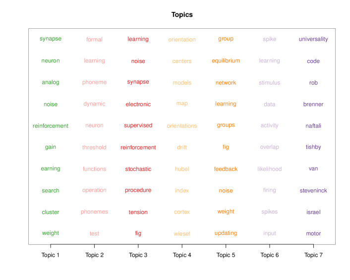
Figure 14: Most specific words for the 5 found topics with STBM on the Nips co-authorship network.

As a conclusive remark on this network, STBM has proved its ability to bring out concise and relevant analyses on the structure of a large and dense network. In this view, the meta-network of Figure 13 is a great help since it summarizes several model parameters of STBM.

6 Conclusion

This work has introduced a probabilistic model, named the stochastic topic bloc model (STBM), for the modeling and clustering of vertices in networks with textual edges. The proposed model allows the modeling of both directed and undirected networks, authorizing its application to networks of various types (communication, social medias, co-authorship, …). A classification variational EM (C-VEM) algorithm has been proposed for model inference and model selection is done through the ICL criterion. Numerical experiments on simulated data sets have proved the effectiveness of the proposed methodology. Two real-world networks (a communication and a co-authorship network) have also been studied using the STBM model and insightful results have been exhibited. It is worth noticing that STBM has been applied to a large co-authorship network with thousands of vertices, proving the scalability of our approach.

Further work may include the extension of the STBM model to dynamic networks and networks with covariate information on the nodes and / or edges. The extension to the dynamic framework would be possible by adding for instance a state space model over group and topics proportions. Such an approach has already been used with success on SBM-like models, such as in Bouveyron et al. (2016). It would also be possible to take into account covariate information available on the nodes by adopting a mixture of experts approach, such as in Gormley and Murphy (2010). Extending the STBM model to overlapping clusters of nodes would be another natural idea. It is indeed commonplace in social analysis to allow individuals to belong to multiple groups (family, work, friends, …). One possible choice would be to derive an extension of the MMSBM model (Airoldi et al., 2008). However, this would increase significantly the parameterization of the model. Finally, STBM could also be adapted in order to take into account the intensity or the type of communications between individuals.

Appendix A Appendix

A.1 Optimization of $R(Z)$

The VEM update step for each distribution $R(Z_{ij}^{dn})$, $A_{ij}=1$, is given by

$$\log R(Z_{ij}^{dn}) =\mathrm{E}_{Z^{\backslash i,j,d,n},\theta}[\log p(W|A,Z,\beta)+\log p(Z|A,Y,\theta)]+\mathrm{const}$$ (9)

$$=\sum_{k=1}^{K}Z_{ij}^{dnk}\sum_{v=1}^{V}W_{ij}^{dnv}\log\beta_{kv}+\sum_{q,r}^{Q}Y_{iq}Y_{jr}\sum_{k=1}^{K}Z_{ij}^{dnk}\mathrm{E}_{\theta_{qr}}[\log\theta_{qrk}]+\mathrm{const}$$

$$=\sum_{k=1}^{K}Z_{ij}^{dnk}\left(\sum_{v=1}^{V}W_{ij}^{dnv}\log\beta_{kv}+\sum_{q,r}^{Q}Y_{iq}Y_{jr}\Big{(}\psi(\gamma_{qrk}-\psi(\sum_{k=1}^{K}\gamma_{qrk})\Big{)}\right)+\mathrm{const},$$

where all terms that do not depend on $Z_{ij}^{dn}$ have been put into the constant term $\mathrm{const}$. Moreover, $\psi(\cdot)$ denotes the digamma function. The functional form of a multinomial distribution is then recognized in (9)

$$R(Z_{ij}^{dn})=\mathcal{M}\left(Z_{ij}^{dn};1,\phi_{ij}^{dn}=(\phi_{ij}^{dn1},\dots,\phi_{ij}^{dnK})\right),$$

where

$$\phi_{ij}^{dnk}\propto\left(\prod_{v=1}^{V}\beta_{kv}^{W_{ij}^{dnv}}\right)\prod_{q,r}^{Q}\exp\Big{(}\psi(\gamma_{qrk}-\psi(\sum_{l=1}^{K}\gamma_{qrl})\Big{)}^{Y_{iq}Y_{jr}}.$$

$\phi_{ij}^{dnk}$ is the (approximate) posterior distribution of words $W_{ij}^{dn}$ being in topic $k$.

A.2 Optimization of $R(\theta)$

The VEM update step for distribution $R(\theta)$ is given by

$$\log R(\theta) =\mathrm{E}_{Z}[\log p(Z|A,Y,\theta)]+\mathrm{const}$$

$$=\sum_{i\neq j}^{M}A_{ij}\sum_{d=1}^{D_{ij}}\sum_{n=1}^{N_{ij}^{d}}\sum_{q,r}^{Q}Y_{iq}Y_{jr}\sum_{k=1}^{K}\mathrm{E}_{Z_{ij}^{dn}}[Z_{ij}^{dnk}]\log\theta_{qrk}+\sum_{q,r}^{Q}\sum_{k=1}^{K}(\alpha_{k}-1)\log\theta_{qrk}+\mathrm{const}$$

$$=\sum_{q,r}^{Q}\sum_{k=1}^{K}\left(\alpha_{k}+\sum_{i\neq j}^{M}A_{ij}Y_{iq}Y_{jr}\sum_{d=1}^{N_{ij}^{d}}\sum_{n=1}^{N_{ij}^{dn}}\phi_{ij}^{dnk}-1\right)\log\theta_{qrk}+\mathrm{const}.$$

We recognize the functional form of a product of Dirichlet distributions

$$R(\theta)=\prod_{q,r}^{Q}\mathrm{Dir}(\theta_{qr};\gamma_{qr}=(\gamma_{qr1},\dots,\gamma_{qrK})),$$

where

$$\gamma_{qrk}=\alpha_{k}+\sum_{i\neq j}^{M}A_{ij}Y_{iq}Y_{jr}\sum_{d=1}^{N_{ij}^{d}}\sum_{n=1}^{N_{ij}^{dn}}\phi_{ij}^{dnk}.$$

A.3 Derivation of the lower bound $\tilde{\mathcal{L}}\left(R(\cdot);Y,\beta\right)$

The lower bound $\tilde{\mathcal{L}}\left(R(\cdot);Y,\beta\right)$ in (7) is given by

$$\tilde{\mathcal{L}}\left(R(\cdot);Y,\beta\right) =\sum_{Z}\int_{\theta}R(Z,\theta)\log\frac{p(W,Z,\theta|A,Y,\beta)}{R(Z,\theta)}d\theta$$ (10)

$$=\mathrm{E}_{Z}[\log p(W|A,Z,\beta)]+\mathrm{E}_{Z,\theta}[\log p(Z|A,Y,\theta)]+\mathrm{E}_{\theta}[\log p(\theta)]-\mathrm{E}_{Z}[\log R(Z)]-\mathrm{E}_{\theta}[\log R(\theta)]$$

$$=\sum_{i\neq j}^{M}A_{ij}\sum_{d=1}^{D_{ij}}\sum_{n=1}^{N_{ij}^{dn}}\sum_{k=1}^{K}\phi_{ij}^{dnk}\sum_{v=1}^{V}W_{ij}^{dnv}\log\beta_{kv}$$

$$\quad\quad+\sum_{i\neq j}^{M}A_{ij}\sum_{d=1}^{D_{ij}}\sum_{n=1}^{N_{ij}^{dn}}\sum_{q,r}^{Q}Y_{iq}Y_{jr}\sum_{k=1}^{K}\phi_{ij}^{dnk}\Big{(}\psi(\gamma_{qrk})-\psi(\sum_{l=1}^{K}\gamma_{qrl})\Big{)}$$

$$\quad\quad+\sum_{q,r}^{Q}\left(\log\Gamma(\sum_{l=1}^{K}\alpha_{k})-\sum_{l=1}^{K}\log\Gamma(\alpha_{l})+\sum_{k=1}^{K}(\alpha_{k}-1)\Big{(}\psi(\gamma_{qrk})-\psi(\sum_{l=1}^{K}\gamma_{qrl})\Big{)}\right)$$

$$\quad\quad-\sum_{i\neq j}^{M}A_{ij}\sum_{d=1}^{D_{ij}}\sum_{n=1}^{N_{ij}^{dn}}\sum_{k=1}^{K}\phi_{ij}^{dnk}\log\phi_{ij}^{dnk}$$

$$\quad\quad-\sum_{q,r}^{Q}\left(\log\Gamma(\sum_{l=1}^{K}\gamma_{qrl})-\sum_{l=1}^{K}\log\Gamma(\gamma_{qrl})+\sum_{k=1}^{K}(\gamma_{qrk}-1)\Big{(}\psi(\gamma_{qrk})-\psi(\sum_{l=1}^{K}\gamma_{qrl})\Big{)}\right)$$

A.4 Optimization of $\beta$

In order to maximize the lower bound $\tilde{\mathcal{L}}\left(R(\cdot);Y,\beta\right)$, we isolate the terms in (10) that depend on $\beta$ and add Lagrange multipliers to satisfy the constraints $\sum_{v=1}^{V}\beta_{kv}=1,\forall k$

$$\tilde{\mathcal{L}}_{\beta}=\sum_{i\neq j}^{M}A_{ij}\sum_{d=1}^{D_{ij}}\sum_{n=1}^{N_{ij}^{dn}}\sum_{k=1}^{K}\phi_{ij}^{dnk}\sum_{v=1}^{V}W_{ij}^{dnv}\log\beta_{kv}+\sum_{k=1}^{K}\lambda_{k}(\sum_{v=1}^{V}\beta_{kv}-1).$$

Setting the derivative, with respect to $\beta_{kv}$, to zero, we find

$$\beta_{kv}\propto\sum_{i\neq j}^{M}A_{ij}\sum_{d=1}^{D_{ij}}\sum_{n=1}^{N_{ij}^{dn}}\phi_{ij}^{dnk}W_{ij}^{dnv}.$$

A.5 Optimization of $\rho$

Only the distribution $p(Y|\rho)$ in the complete data log-likelihood $\log p(A,Y|\rho,\pi)$ depends on the parameter vector $\rho$ of cluster proportions. Taking the log and adding a Lagrange multiplier to satisfy the constraint $\sum_{q=1}^{Q}\rho_{q}=1$, we have

$$\log p(Y|\rho)=\sum_{i=1}^{M}\sum_{q=1}^{Q}Y_{iq}\log\rho_{q}.$$

Taking the derivative with respect $\rho$ to zero, we find

$$\rho_{q}\propto\sum_{i=1}^{M}Y_{iq}.$$

A.6 Optimization of $\pi$

Only the distribution $p(A|Y,\pi)$ in the complete data log-likelihood $\log p(A,Y|\rho,\pi)$ depends on the parameter matrix $\pi$ of connection probabilities. Taking the log we have

$$\log p(A|Y,\pi)=\sum_{i\neq j}^{M}\sum_{q,r}^{Q}Y_{iq}Y_{jr}\Big{(}A_{ij}\log\pi_{qr}+(1-A_{ij})\log(1-\pi_{qr})\Big{)}.$$

Taking the derivative with respect to $\pi_{qr}$ to zero, we obtain

$$\pi_{qr}=\frac{\sum_{i\neq j}^{M}\sum_{q,r}^{Q}Y_{iq}Y_{jr}A_{ij}}{\sum_{i\neq j}^{M}\sum_{q,r}^{Q}Y_{iq}Y_{jr}}.$$

A.7 Model selection

Assuming that the prior distribution over the model parameters $(\rho,\pi,\beta)$ can be factorized, the integrated complete data log-likelihood $\log p(A,W,Y|K,Q)$ is given by

$$\log p(A,W,Y|K,Q) =\log\int_{\rho,\pi,\beta}p(A,W,Y,\rho,\pi,\beta|K,Q)d\rho d\pi d\theta$$

$$=\log\int_{\rho,\pi,\beta}p(A,W,Y|\rho,\pi,\beta,K,Q)p(\rho|Q)p(\pi|Q)p(\beta|K)d\rho d\pi d\beta.$$

Note that the dependency on $K$ and $Q$ is made explicit here, in all expressions. In all other sections of the paper, we did not include these terms to keep the notations uncluttered. We find

$$\log p(A,W,Y|K,Q) =\log\int_{\rho,\pi,\beta}\left(\sum_{Z}\int_{\theta}p(A,W,Y,Z,\theta|\rho,\pi,\beta,K,Q)d\theta\right)p(\rho|Q)p(\pi|Q)p(\beta|K)d\rho d\pi d\beta$$ (11)

$$=\log\int_{\rho,\pi,\beta}\left(\sum_{Z}\int_{\theta}p(W,Z,\theta|A,Y,\beta,K,Q)p(A,Y|\rho,\pi,Q)d\theta\right)p(\rho|Q)p(\pi|Q)p(\beta|K)d\rho d\pi d\beta$$

$$=\log\int_{\rho,\pi,\beta}p(W|A,Y,\beta,K,Q)p(A|Y,\pi,Q)p(Y|\rho,Q)p(\rho|Q)p(\pi|Q)p(\beta|K)d\rho d\pi d\beta$$

$$=\log\int_{\beta}p(W|A,Y,\beta,K,Q)p(\beta|K)d\beta+\log\int_{\pi}p(A|Y,\pi,Q)p(\pi|Q)d\pi$$

$$\quad\quad+\log\int_{\rho}p(Y|\rho,Q)p(\rho|Q)d\rho.$$

Following the derivation of the ICL criterion, we apply a Laplace (BIC-like) approximation on the second term of Equation (11). Moreover, considering a Jeffreys prior distribution for $\rho$ and using Stirling formula for large values of $M$, we obtain

$$\log\int_{\pi}p(A|Y,\pi,Q)p(\pi|Q)d\pi\approx\max_{\pi}\log p(A|Y,\pi,Q)-\frac{Q^{2}}{2}\log M(M-1),$$

as well as

$$\log\int_{\rho}p(Y|\rho,Q)p(\rho|Q)d\rho\approx\max_{\rho}\log p(Y|\rho,Q)-\frac{Q-1}{2}\log M.$$

For more details, we refer to Biernacki et al. (2000). Furthermore, we emphasize that adding these two approximations leads to the ICL criterion for the SBM model, as derived by Daudin et al. (2008)

$$ICL_{SBM} =\max_{\pi}\log p(A|Y,\pi,Q)-\frac{Q^{2}}{2}\log M(M-1)+\max_{\rho}\log p(Y|\rho,Q)-\frac{Q-1}{2}\log M$$

$$=\max_{\rho,\pi}\log p(A,Y|\rho,\pi,Q)-\frac{Q^{2}}{2}\log M(M-1)-\frac{Q-1}{2}\log M.$$

In Daudin et al. (2008), $M(M-1)$ is replaced by $M(M-1)/2$ and $Q^{2}$ by $Q(Q+1)/2$ since they considered undirected networks.

Now, it is worth taking a closer look at the first term of Equation (11). This term involves a marginalization over $\beta$. Let us emphasize that $p(W|A,Y,\beta,K,Q)$ is related to the LDA model and involves a marginalization over $\theta$ (and $Z$). Because we aim at approximating the first term of Equation (11), also with a Laplace (BIC-like) approximation, it is crucial to identify the number of observations in the associated likelihood term $p(W|A,Y,\beta,K,Q)$. As pointed out in Section 2.4, given $Y$ (and $\theta$), it is possible to reorganize the documents in $W$ as $W=(\tilde{W}_{qr})_{qr}$ is such a way that all words in $\tilde{W}_{qr}$ follow the same mixture distribution over topics. Each aggregated document $\tilde{W}_{qr}$ has its own vector $\theta_{qr}$ of topic proportions and since the distribution over $\theta$ factorizes ($p(\theta)=\prod_{q,r}^{Q}p(\theta_{qr}))$, we find

$$p(W|A,Y,\beta,K,Q) =\int_{\theta}p(W|A,Y,\theta,\beta,K,Q)p(\theta|K,Q)d\theta$$

$$=\prod_{q,r}^{Q}\int_{\theta_{qr}}p(\tilde{W}_{qr}|\theta_{qr},\beta,K,Q)p(\theta_{qr}|K)d\theta_{qr}$$

$$=\prod_{q,r}^{Q}\ell(\tilde{W}_{qr}|\beta,K,Q),$$

where $\ell(\tilde{W}_{qr}|\beta,K,Q)$ is exactly the likelihood term of the LDA model associated with document $\tilde{W}_{qr}$, as described in Blei et al. (2003). Thus

$$\log\int_{\beta}p(W|A,Y,\beta,K,Q)p(\beta|K)d\beta=\log\int_{\beta}p(\beta|K)\prod_{q,r}^{Q}\ell(\tilde{W}_{qr}|\beta,K,Q)d\beta.$$ (12)

Applying a Laplace approximation on Equation (12) is then equivalent to deriving a BIC-like criterion for the LDA model with documents in $W=(\tilde{W}_{qr})_{qr}$. In the LDA model, the number of observations in the penalization term of BIC is the number of documents (see Than and Ho, 2012, for instance). In our case, this leads to

$$\log\int_{\beta}p(W|A,Y,\beta,K,Q)p(\beta|K)d\beta\approx\max_{\beta}\log p(W|A,Y,\beta,K,Q)-\frac{K(V-1)}{2}\log Q^{2}.$$ (13)

Unfortunately, $\log p(W|A,Y,\beta,K,Q)$ is not tractable and so we propose to replace it with its variational approximation $\tilde{\mathcal{L}}$, after convergence of the C-VEM algorithm. By analogy with $ICL_{SBM}$, we call the corresponding criterion $BIC_{LDA|Y}$ such that

$$\log p(A,W,Y|K,Q)\approx BIC_{LDA|Y}+ICL_{SBM}.$$

References

- Airoldi et al. (2008) Airoldi, E., Blei, D., Fienberg, S. and Xing, E. (2008). Mixed membership stochastic blockmodels. The Journal of Machine Learning Research. 9 1981–2014.
- Akaike (1973) Akaike, H. (1973). Information theory and an extension of the maximum likelihood principle. In Second International Symposium on Information Theory, 267–281.
- Ambroise et al. (2010) Ambroise, C., Grasseau, G., Hoebeke, M., Latouche, P., Miele, V. and Picard, F., (2010). The mixer R package (version 1.8). http://cran.r-project.org/web/packages/mixer/.
- Bickel and Chen (2009) Bickel, P. and Chen, A. (2009). A nonparametric view of network models and newman–girvan and other modularities. Proceedings of the National Academy of Sciences. 106 (50) 21068–21073.
- Biernacki et al. (2000) Biernacki, C., Celeux, G. and Govaert, G. (2000). Assessing a mixture model for clustering with the integrated completed likelihood. IEEE Trans. Pattern Anal. Machine Intel. 7 719–725.
- Biernacki et al. (2003) Biernacki, C., Celeux, G. and Govaert, G. (2003). Choosing starting values for the EM algorithm for getting the highest likelihood in multivariate gaussian mixture models. Computational Statistics and Data Analysis. 41 (3-4) 561–575.
- Bilmes (1998) Bilmes, J. (1998). A gentle tutorial of the EM algorithm and its application to parameter estimation for gaussian mixture and hidden markov models. International Computer Science Institute. 4 126.
- Blei and Lafferty (2006) Blei, D. and Lafferty, J. (2006). Correlated topic models. Advances in neural information processing systems. 18 147.
- Blei (2012) Blei, D. M. (2012). Probabilistic topic models. Communications of the ACM. 55 (4) 77–84.
- Blei et al. (2003) Blei, D. M., Ng, A. Y. and Jordan, M. I. (2003). Latent dirichlet allocation. the Journal of machine Learning research. 3 993–1022.
- Blondel et al. (2008) Blondel, V. D., Guillaume, J.-L., Lambiotte, R. and Lefebvre, E. (2008). Fast unfolding of communities in large networks. Journal of Statistical Mechanics: Theory and Experiment. 10 10008–10020.
- Bouveyron et al. (2016) Bouveyron, C., Latouche, P. and Zreik, R. (2016). The dynamic random subgraph model for the clustering of evolving networks. Computational Statistics. in press.
- Celeux and Govaert (1991) Celeux, G. and Govaert, G. (1991). A classification em algorithm for clustering and two stochastic versions. Computational Statistics Quaterly. 2 (1) 73–82.
- Chang and Blei (2009) Chang, J. and Blei, D. M. (2009). Relational topic models for document networks. In International Conference on Artificial Intelligence and Statistics, 81–88.
- Côme and Latouche (2015) Côme, E. and Latouche, P. (2015). Model selection and clustering in stochastic block models with the exact integrated complete data likelihood. Statistical Modelling. to appear.
- Côme et al. (2014) Côme, E., Randriamanamihaga, A., Oukhellou, L. and Aknin, P. (2014). Spatio-temporal analysis of dynamic origin-destination data using latent dirichlet allocation. application to the vélib? bike sharing system of paris. In In Proceedings of 93rd Annual Meeting of the Transportation Research Board.
- Daudin et al. (2008) Daudin, J.-J., Picard, F. and Robin, S. (2008). A mixture model for random graphs. Statistics and Computing. 18 (2) 173–183.
- Deerwester et al. (1990) Deerwester, S., Dumais, S., Furnas, G., Landauer, T. and Harshman, R. (1990). Indexing by latent semantic analysis. Journal of the American society for information science. 41 (6) 391.
- Dempster et al. (1977) Dempster, A., Laird, N. and Rubin, D. (1977). Maximum likelihood from incomplete data via the EM algorithm. Journal of the Royal Statistical Society. Series B (Methodological). 1–38.
- Fienberg and Wasserman (1981) Fienberg, S. and Wasserman, S. (1981). Categorical data analysis of single sociometric relations. Sociological Methodology. 12 156–192.
- Girvan and Newman (2002) Girvan, M. and Newman, M. (2002). Community structure in social and biological networks. Proceedings of the National Academy of Sciences. 99 (12) 7821.
- Gormley and Murphy (2010) Gormley, I. C. and Murphy, T. B. (2010). A mixture of experts latent position cluster model for social network data. Statistical methodology. 7 (3) 385–405.
- Grun and Hornik (2013) Grun, B. and Hornik, K., (2013). The mixer topicmodels package (version 0.2-3). http://cran.r- project.org/web/packages/topicmodels/.
- Handcock et al. (2007) Handcock, M., Raftery, A. and Tantrum, J. (2007). Model-based clustering for social networks. Journal of the Royal Statistical Society: Series A (Statistics in Society). 170 (2) 301–354.
- Hathaway (1986) Hathaway, R. (1986). Another interpretation of the EM algorithm for mixture distributions. Statistics & Probability Letters. 4 (2) 53–56.
- Hoff et al. (2002) Hoff, P., Raftery, A. and Handcock, M. (2002). Latent space approaches to social network analysis. Journal of the American Statistical Association. 97 (460) 1090–1098.
- Hofman and Wiggins (2008) Hofman, J. and Wiggins, C. (2008). Bayesian approach to network modularity. Physical review letters. 100 (25) 258701.
- Hofmann (1999) Hofmann, T. (1999). Probabilistic latent semantic indexing. In Proceedings of the 22nd annual international ACM SIGIR conference on Research and development in information retrieval, 50–57. ACM.
- Jernite et al. (2014) Jernite, Y., Latouche, P., Bouveyron, C., Rivera, P., Jegou, L. and Lamassé, S. (2014). The random subgraph model for the analysis of an acclesiastical network in merovingian gaul. Annals of Applied Statistics. 8 (1) 55–74.
- Kemp et al. (2006) Kemp, C., Tenenbaum, J., Griffiths, T., Yamada, T. and Ueda, N. (2006). Learning systems of concepts with an infinite relational model. In Proceedings of the National Conference on Artificial Intelligence, volume 21, 381–391.
- Latouche et al. (2011) Latouche, P., Birmelé, E. and Ambroise, C. (2011). Overlapping stochastic block models with application to the french political blogosphere. Annals of Applied Statistics. 5 (1) 309–336.
- Latouche et al. (2012) Latouche, P., Birmelé, E. and Ambroise, C. (2012). Variational bayesian inference and complexity control for stochastic block models. Statistical Modelling. 12 (1) 93–115.
- Lazebnik et al. (2006) Lazebnik, S., Schmid, C. and Ponce, J. (2006). Beyond bags of features: Spatial pyramid matching for recognizing natural scene categories. In Computer Vision and Pattern Recognition, 2006 IEEE Computer Society Conference on, volume 2, 2169–2178. IEEE.
- Liu et al. (2009) Liu, Y., Niculescu-Mizil, A. and Gryc, W. (2009). Topic-link lda: joint models of topic and author community. In proceedings of the 26th annual international conference on machine learning, 665–672. ACM.
- Mariadassou et al. (2010) Mariadassou, M., Robin, S. and Vacher, C. (2010). Uncovering latent structure in valued graphs: a variational approach. Annals of Applied Statistics. 4 (2) 715–742.
- Matias and Miele (2016) Matias, C. and Miele, V. (2016). Statistical clustering of temporal networks through a dynamic stochastic block model. Preprint HAL. n.01167837.
- Matias and Robin (2014) Matias, C. and Robin, S. (2014). Modeling heterogeneity in random graphs through latent space models: a selective review. Esaim Proc. and Surveys. 47 55–74.
- Mc Daid et al. (2013) Mc Daid, A., Murphy, T., N., F. and Hurley, N. (2013). Improved bayesian inference for the stochastic block model with application to large networks. Computational Statistics and Data Analysis. 60 12–31.
- McCallum et al. (2005) McCallum, A., Corrada-Emmanuel, A. and Wang, X. (2005). The author-recipient-topic model for topic and role discovery in social networks, with application to enron and academic email. In Workshop on Link Analysis, Counterterrorism and Security, 33–44.
- Newman (2004) Newman, M. E. J. (2004). Fast algorithm for detecting community structure in networks. Physical Review Letter E. 69 0066133.
- Nigam et al. (2000) Nigam, K., McCallum, A., Thrun, S. and Mitchell, T. (2000). Text classification from labeled and unlabeled documents using em. Machine learning. 39 (2-3) 103–134.
- Nowicki and Snijders (2001) Nowicki, K. and Snijders, T. (2001). Estimation and prediction for stochastic blockstructures. Journal of the American Statistical Association. 96 (455) 1077–1087.
- Papadimitriou et al. (1998) Papadimitriou, C., Raghavan, P., Tamaki, H. and Vempala, S. (1998). Latent semantic indexing: A probabilistic analysis. In Proceedings of the tenth ACM PODS, 159–168. ACM.
- Pathak et al. (2008) Pathak, N., DeLong, C., Banerjee, A. and Erickson, K. (2008). Social topic models for community extraction. In The 2nd SNA-KDD workshop, volume 8. Citeseer.
- Rand (1971) Rand, W. (1971). Objective criteria for the evaluation of clustering methods. Journal of the American Statistical association. 846–850.
- Rosen-Zvi et al. (2004) Rosen-Zvi, M., Griffiths, T., Steyvers, M. and Smyth, P. (2004). The author-topic model for authors and documents. In Proceedings of the 20th conference on Uncertainty in artificial intelligence, 487–494. AUAI Press.
- Sachan et al. (2012) Sachan, M., Contractor, D., Faruquie, T. and Subramaniam, L. (2012). Using content and interactions for discovering communities in social networks. In Proceedings of the 21st international conference on World Wide Web, 331–340. ACM.
- Salter-Townshend et al. (2012) Salter-Townshend, M., White, A., Gollini, I. and Murphy, T. B. (2012). Review of statistical network analysis: models, algorithms, and software. Statistical Analysis and Data Mining. 5 (4) 243–264.
- Schwarz (1978) Schwarz, G. (1978). Estimating the dimension of a model. Annals of Statistics. 6 461–464.
- Steyvers et al. (2004) Steyvers, M., Smyth, P., Rosen-Zvi, M. and Griffiths, T. (2004). Probabilistic author-topic models for information discovery. In Proceedings of the tenth ACM SIGKDD international conference on Knowledge discovery and data mining, 306–315. ACM.
- Sun et al. (2009) Sun, Y., Han, J., Gao, J. and Yu, Y. (2009). itopicmodel: Information network-integrated topic modeling. In Data Mining, 2009. ICDM’09. Ninth IEEE International Conference on, 493–502. IEEE.
- Teh et al. (2006) Teh, Y., Newman, D. and Welling, M. (2006). A collapsed variational bayesian inference algorithm for latent Dirichlet allocation. Advances in neural information processing systems. 18 1353–1360.
- Than and Ho (2012) Than, K. and Ho, T. (2012). Machine Learning and Knowledge Discovery in Databases, Lecture Notes in Computer Science. volume 7523, chapter Fully sparse topic models, 490–505. Springer.
- Wang and Wong (1987) Wang, Y. and Wong, G. (1987). Stochastic blockmodels for directed graphs. Journal of the American Statistical Association. 82 8–19.
- White et al. (1976) White, H., Boorman, S. and Breiger, R. (1976). Social structure from multiple networks. i. blockmodels of roles and positions. American Journal of Sociology. 730–780.
- Xu and Hero III (2013) Xu, K. and Hero III, A. (2013). Dynamic stochastic blockmodels: Statistical models for time-evolving networks. In Social Computing, Behavioral-Cultural Modeling and Prediction, 201–210. Springer.
- Yang et al. (2011) Yang, T., Chi, Y., Zhu, S., Gong, Y. and Jin, R. (2011). Detecting communities and their evolutions in dynamic social networks: a bayesian approach. Machine learning. 82 (2) 157–189.
- Zanghi et al. (2008) Zanghi, H., Ambroise, C. and Miele, V. (2008). Fast online graph clustering via erdos-renyi mixture. Pattern recognition. 41 3592–3599.
- Zanghi et al. (2010) Zanghi, H., Volant, S. and Ambroise, C. (2010). Clustering based on random graph model embedding vertex features. Pattern Recognition Letters. 31 (9) 830–836.
- Zhou et al. (2006) Zhou, D., Manavoglu, E., Li, J., Giles, C. and Zha, H. (2006). Probabilistic models for discovering e-communities. In Proceedings of the 15th international conference on World Wide Web, 173–182. ACM.