Interplay of Site and Bond Electron-Phonon Coupling in One Dimension

Abstract

The interplay of bond and charge correlations is studied in a one-dimensional model with both Holstein and Su-Schrieffer-Heeger (SSH) couplings to quantum phonons. The problem is solved exactly by quantum Monte Carlo simulations. If one of the couplings dominates, the ground state is a Peierls insulator with long-range bond or charge order. At weak coupling, the results suggest a spin-gapped and repulsive metallic phase arising from the competing order parameters and lattice fluctuations. Such a phase is absent from the pure SSH model even for quantum phonons. At strong coupling, evidence for a continuous transition between the two Peierls states is presented.

Electron-phonon coupling is at the heart of phenomena such as polaron formation, the Peierls instability, superconductivity, and relaxation in nonequilibrium. At the same time, a correct quantum mechanical treatment poses a serious challenge even for modern numerical methods. The rich physics arising from the fundamental Holstein density-displacement [1] or Su-Schrieffer-Heeger (SSH) hopping-displacement coupling [2] has been studied in great detail . However, their interplay is so far unexplored , even though both couplings will typically be present in materials [5].

For a half-filled band in one dimension with Fermi wave vector $k_{\text{F}}=\pi/2$, a Holstein coupling causes a Peierls transition to a $2k_{\text{F}}$ charge-density-wave (CDW) insulator at a critical coupling $\lambda_{\text{s}}^{c}>0$, as illustrated in Fig. 1. In contrast to mean-field theory, quantum lattice fluctuations destroy the Peierls state for $\lambda_{\text{s}}<\lambda_{\text{s}}^{c}$ and produce a spin-gapped metallic phase [6]. On the other hand, the $2k_{\text{F}}$ bond-order wave (BOW) Peierls state of the (spinful) SSH model—with alternating weak and strong bonds—is stable for any $\lambda_{\text{b}}>0$ [7; 8; 9; 10; 11]. Hence, in this case, Peierls's theorem [12] holds beyond the adiabatic limit. Different components of the retarded phonon-mediated interactions give rise to the spin gap and the Peierls state. Even a qualitatively correct understanding of these models is beyond the widely used adiabatic and antiadiabatic approximations or even the bosonization, and instead requires advanced methods [10; 13]. More realistic models with both interactions have so far not been studied.

The competition between interactions in the presence of lattice fluctuations is complex. Whereas metallic behavior arises from competing electron-electron and Holstein electron-phonon interactions [14; 15], SSH models only support Peierls and Mott states [8; 10; 11]. In contrast to the simpler yet intricate extended Hubbard model [16; 17; 18; 19], there are no nontrivial integrable limiting cases in the electron-phonon problem. Two key questions are if a metallic phase can emerge from the interplay of CDW and BOW order, and how the transition between the different Peierls states takes place.

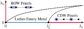
Figure 1: Schematic phase diagram of the model (Interplay of Site and Bond Electron-Phonon Coupling in One Dimension). Dots indicate critical points of the Holstein and SSH models, dashed lines illustrate the expected phase boundaries.

In this Letter, we study this problem by exact quantum Monte Carlo simulations of the Hamiltonian

$$\hat{H} =-t\sum_{i}\hat{B}_{i}+\sum_{i,\alpha}\left[\mbox{$\frac{1}{2M_{\alpha}}$}\hat{P}^{2}_{i,\alpha}+\mbox{$\frac{K_{\alpha}}{2}$}\hat{Q}_{i,\alpha}^{2}\right]$$

$$\phantom{=}-g_{\text{s}}\sum_{i}(\hat{n}_{i}-1)\hat{Q}_{i,\text{s}}-g_{\text{b}}\sum_{i}\hat{B}_{i}\hat{Q}_{i,\text{b}}\,.$$ (1)

The bond operator $\hat{B}_{i}=\sum_{\sigma}(\hat{c}^{\dagger}_{i\sigma}\hat{c}^{\phantom{{\dagger}}}_{i+1\sigma}+\hat{c}^{\dagger}_{i+1\sigma}\hat{c}^{\phantom{{\dagger}}}_{i\sigma})$, where $\hat{c}^{\dagger}_{i\sigma}$ creates an electron with spin $\sigma$ at lattice site $i$, and the density operator $\hat{n}_{i}=\sum_{\sigma}c^{\dagger}_{i\sigma}c^{\phantom{{\dagger}}}_{i\sigma}$. The first term in Eq. (Interplay of Site and Bond Electron-Phonon Coupling in One Dimension) describes the hopping of electrons between neighboring lattice sites with amplitude $t$. The second term models harmonic oscillations on site or bond $i$, with $M_{\alpha}$ and $K_{\alpha}$ the mass and stiffness constant associated with the independent site ($\alpha=\text{s}$) and bond phonons ($\alpha=\text{b}$), respectively. The third (fourth) term is a Holstein (SSH) coupling to site (bond) displacements $\hat{Q}_{i,\text{s}}$ ($\hat{Q}_{i,\text{b}}$). Equation (Interplay of Site and Bond Electron-Phonon Coupling in One Dimension) reduces to the Holstein model for $\lambda_{\text{b}}=0$, and to the optical SSH model for $\lambda_{\text{s}}=0$. The latter gives the same results as the SSH model with acoustic phonons and a coupling $g_{\text{b}}\sum_{i}\hat{B}_{i}(\hat{Q}_{i+1,\text{b}}-\hat{Q}_{i,\text{b}})$ but has no sign problem [11]. In terms of the $g_{\alpha}$, the coupling constants $\lambda_{\alpha}$ are given by $\lambda_{\text{s}}=g_{\text{s}}^{2}/(4K_{\text{s}}t)$ and $\lambda_{\text{b}}=g_{\text{b}}^{2}/(K_{\text{b}}t)$, respectively. We take the phonon frequencies $\omega_{0,\alpha}=\sqrt{K_{\alpha}/M_{\alpha}}$ to be equal, $\omega_{0,\alpha}=\omega_{0}=0.5t$, set $\hbar=k_{\text{B}}=1$, and consider half-filled ($\langle\hat{n}_{i}\rangle=1$, chemical potential $\mu=0$) periodic chains with $L$ sites at inverse temperature $\beta t=t/T=L$.

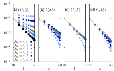
Figure 2: (a) Bond, (b) charge, (c) pairing, (d) spin correlations as a function of the conformal distance $\xi$ (see text). Here, $\lambda_{\text{s}}=0.15<\lambda_{\text{s}}^{c}$, $L=50$. Solid lines illustrate a $r^{-2}$ decay.

Hamiltonian (Interplay of Site and Bond Electron-Phonon Coupling in One Dimension) represents a significant challenge due to the different time scales for the dynamics of electrons and phonons and the infinite bosonic Hilbert space. It can be simulated with the continuous-time quantum Monte Carlo method of Ref. [20] which is based on the exact summation of a weak-coupling expansion of the partition function. A key advantage of this method is that its path-integral formulation permits integrating out the phonons and simulating an effective fermionic model [21] that captures the full dynamics of the quantum phonons. The resulting retarded interactions have the form $S^{1}_{\alpha}=-\gamma^{2}_{\alpha}\iint_{0}^{\beta}\text{d}\tau\text{d}\tau^{\prime}\sum_{q}\overline{\rho}_{\alpha}(q,\tau)D^{0}_{\alpha}(q,\tau-\tau^{\prime})\rho_{\alpha}(q,\tau^{\prime})$, where $D^{0}_{\alpha}$ is the free phonon propagator; $\rho_{\alpha}(q,\tau)$ is a Grassmann bilinear corresponding to the Fourier transform of the bond operator $\hat{B}_{i}$ (for $\alpha=\text{b}$) or the charge operator $\hat{n}_{i}$ (for $\alpha=\text{s}$), respectively. As in previous work, we used single-vertex updates and Ising spin flips [21]. To calculate spectral functions, we applied a maximum-entropy method for the analytic continuation [22].

Theoretical expectations.—Luttinger liquid theory describes one-dimensional systems in terms of charge or spin Luttinger parameters $K_{\rho/\sigma}$ and velocities $v_{\rho/\sigma}$ [23]. Whereas the metallic phase of the Holstein model is only captured if the momentum and frequency dependence of the interaction is taken into account [10], the simple g-ology representation in terms of backward ($g_{1}$), forward ($g_{2}$), and umklapp ($g_{3}$) scattering [23] already reveals important differences to the SSH model. Whereas $g_{2}$ terms only renormalize the quadratic theory, $g_{1}$ and $g_{3}$ have the potential to open gaps and/or break symmetries if relevant in the renormalization group sense [23]. The Holstein coupling gives $g_{\text{1,s}}=g_{\text{2,s}}=g_{\text{3,s}}=-2g_{\text{s}}^{2}/\omega_{0,\text{s}}$, whereas the SSH coupling leads to $g_{\text{1,b}}=-g_{\text{3,b}}=-2g_{\text{b}}^{2}/\omega_{0,\text{b}}$, and $g_{\text{2,b}}=0$ [10]. In the combined model (Interplay of Site and Bond Electron-Phonon Coupling in One Dimension) the backscattering $g_{1}=g_{\text{1,s}}+g_{\text{1,b}}$ is always attractive, whereas the total umklapp matrix element $g_{3}=g_{\text{3,s}}+g_{\text{3,b}}$ can be small or zero for suitable $g_{\text{s}}$ and $g_{\text{b}}$ (or $\lambda_{\text{s}}$ and $\lambda_{\text{b}}$).

As in the attractive Hubbard model, any $g_{1}<0$ opens a spin gap in Holstein and SSH models [24; 11]. The relevance of umklapp scattering for any $\lambda_{\text{b}}>0$ in the SSH model has been attributed to the vanishing of $g_{\text{2,b}}$ [10]. In contrast, weak umklapp scattering is irrelevant in the Holstein model and gives a metallic Luther-Emery phase with a gap for single-particle and spin excitations but gapless charge excitations [6; 14; 15; 24; 13]. The model (Interplay of Site and Bond Electron-Phonon Coupling in One Dimension) should permit metallic behavior due to $g_{2}\neq 0$ and the compensation of $g_{\text{3,s}}$ and $g_{\text{3,b}}$. Similarly, attractive umklapp scattering is compensated by repulsive contributions from the electron-electron interaction in the Holstein-Hubbard model [14], whereas all $g_{3}$ terms are positive in the SSH-Hubbard model for polyacetylene [10]. Finally, the Peierls states break a discrete Ising symmetry at $T=0$, allowing for long-range order.

Weak site coupling.—We first consider the impact of the SSH coupling on the metallic phase of the Holstein model with $\lambda_{\text{s}}=0.15<\lambda_{\text{s}}^{c}\approx 0.25$ [25; 15; 13]. Figure 2 shows the correlators $C_{\text{b}}(r)=\langle\hat{B}_{r}\hat{B}_{0}\rangle-\langle\hat{B}_{r}\rangle^{2}$, $C_{\rho}(r)=\langle(\hat{n}_{r}-1)(\hat{n}_{0}-1)\rangle$, $C_{\text{p}}(r)=\langle c^{\phantom{{\dagger}}}_{r\uparrow}c^{\phantom{{\dagger}}}_{r\downarrow}c^{\dagger}_{0\uparrow}c^{\dagger}_{0\downarrow}\rangle$, and $C_{\sigma}(r)=\langle\hat{s}^{x}_{r}\hat{s}^{x}_{0}\rangle$ ($\hat{s}^{x}_{r}=c^{\dagger}_{r\uparrow}c^{\phantom{{\dagger}}}_{r\downarrow}+c^{{\dagger}}_{r\downarrow}c^{\phantom{{\dagger}}}_{r\uparrow}$) as a function of the conformal distance $\xi=L\sin({\pi r}/{L})$ [26]. Starting from dominant CDW correlations at $\lambda_{\text{b}}=0$, CDW (BOW) correlations are suppressed (enhanced) with increasing $\lambda_{\text{b}}$. At the same time, pairing is slightly enhanced [Fig. 2(c)]. All three channels initially retain a power-law form, compatible with a metallic phase. For larger $\lambda_{\text{b}}$ we observe long-range bond order, and exponentially decaying charge, pairing, and spin correlations. The different decay of charge (or bond) and spin correlations implies a spin gap for all $\lambda_{\text{b}}$: In a gapless Luttinger liquid the $2k_{\text{F}}$ part of all three correlators decays with exponent $K_{\rho}+K_{\sigma}$ [27]. In contrast, in a Luther-Emery liquid, the exponent is $K_{\rho}$ for bond/charge ($K_{\rho}^{-1}$ for pairing) while spin correlations decay exponentially . The dominance of bond over pairing correlations indicates effectively repulsive interactions ($K_{\rho}<1$).

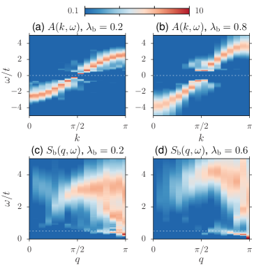
Figure 3: (a)–(b) Single-particle spectral function, and (c)–(d) dynamic bond structure factor. Here, $\lambda_{\text{s}}=0.15<\lambda_{\text{s}}^{c}$, and $L=30$. Dashed lines indicate $\omega=0$ and $\omega=\omega_{0}$, respectively.

The transition to the BOW-Peierls phase is also reflected in the excitation spectra shown in Fig. 3. For $\lambda_{\text{b}}=0.2$ [Fig. 3(a)], the single-particle spectral function reveals a small spin gap at the Fermi level. The electron-phonon coupling significantly broadens the excitations outside the coherent interval $|\omega|<\omega_{0}$ [30; 31]. A clear Peierls gap can be seen for $\lambda_{\text{b}}=0.8$ [Fig. 3(b)]. The bond phonon dispersion is visible in the dynamic bond structure factor $S_{\text{b}}(q,\omega)$ , in addition to signatures of the particle-hole continuum. For $\lambda_{\text{b}}=0.2$ [Fig. 3(c)] the mode is slightly softened near the zone boundary, whereas the complete softening for $\lambda_{\text{b}}=0.6$ [Fig. 3(d)] is consistent with long-range bond order.

Strong site coupling.—We now consider the effect of the bond coupling on the CDW Peierls state at $\lambda_{\text{s}}=0.3$. For $\lambda_{\text{b}}=0$ we have long-range charge order [Fig. 4(b)] and exponential bond, pairing, and spin correlations. A nonzero bond coupling enhances bond correlations, whereas charge correlations are suppressed until they closely follow the free-fermion result $1/r^{2}$ for $\lambda_{\text{b}}=0.5$. The pairing and spin correlations are enhanced at intermediate $\lambda_{\text{b}}$, but remain exponential.

The single-particle spectral function is shown in Fig. 5 for $\lambda_{\text{s}}=0.4$. For weak bond coupling $\lambda_{\text{b}}=0.2$, the spectrum in Fig. 5(a) exhibits the key features of a Peierls insulator, namely a gap at the Fermi level, backfolded shadow bands, and soliton excitations inside the mean-field gap [33; 31]. Remarkably, for $\lambda_{\text{b}}=0.6$ [Fig. 5(b)], the Peierls features are strongly suppressed and the spectrum closely resembles that of Fig. 3(a), despite the strong bare couplings. The corresponding bond and charge structure factors are discussed below.

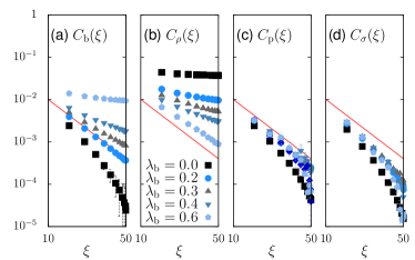
Figure 4: As in Fig. 2 but for $\lambda_{\text{s}}=0.3>\lambda_{\text{s}}^{c}$.

Metallic phase and CDW-BOW transition.—To substantiate metallic behavior at weak coupling, we consider the bond correlations at the largest distance $L/2$, which serve as an order parameter for the Peierls transition. Figure 6(a) illustrates that at $\lambda_{\text{b}}=0.1$ these correlations are smaller for $\lambda_{\text{s}}>0$ than for $\lambda_{\text{s}}=0$ for each $L$. While the extrapolation $L\to\infty$ is nontrivial [11], the suppression of $2k_{\text{F}}$ bond order together with the absence of CDW order in the Holstein model for $\lambda_{\text{s}}=0.15$ and the power-law decay of bond, charge, and pairing correlations (Fig. 2) all indicate metallic behavior in the weak-coupling regime of the phase diagram. The Holstein coupling hence stabilizes the system against the BOW-Peierls transition of the SSH model.

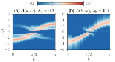
Figure 5: Single-particle spectral function for $\lambda_{\text{s}}=0.4$, $L=30$. Here, (a) $\lambda_{\text{b}}=0.2$ and (b) $\lambda_{\text{b}}=0.6$.

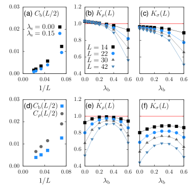
Figure 6: (a) Bond correlations for $r=L/2$, $\lambda_{\text{b}}=0.1$. (b)–(c), (e)–(f) Finite-size estimates of the Luttinger parameters $K_{\rho}$ and $K_{\sigma}$. (d) Bond and charge correlations for $r=L/2$, $\lambda_{\text{b}}=0.4$. Here, $\lambda_{\text{s}}=0.15$ in (b)–(c) and $\lambda_{\text{s}}=0.3$ in (d)–(f).

The exact determination of $K_{\rho}$ and $K_{\sigma}$ is problematic for Luther-Emery liquids [13]. However, even the qualitative behavior yields important insights. The usual finite-size estimates $K_{\rho/\sigma}(L)=\pi C_{\rho/\sigma}(q_{1})/q_{1}$ (with $q_{1}=2\pi/L$) are shown in Figs. 6(b)–(c) for $\lambda_{\text{s}}=0.15$. We have $K_{\rho}(L)\gtrsim 1$ for small $\lambda_{\text{b}}$ although pairing correlations are subdominant (Fig. 2). This mismatch is due to the spin gap that causes a logarithmic convergence with $L$ [13]. At larger $\lambda_{\text{b}}$, $K_{\rho}(L)$ is suppressed and scales to zero for $L\to\infty$. Given the SU(2) spin symmetry of Hamiltonian (Interplay of Site and Bond Electron-Phonon Coupling in One Dimension) we expect $K_{\sigma}=1$ for a Luttinger liquid [23]. Instead, $K_{\sigma}(L)<1$ implies a nonzero spin gap [34] even if the latter is too small to be visible from the spin correlation functions. The results for $K_{\rho/\sigma}(L)$ in Fig. 6(b) resemble those for the Holstein model [14; 13], and support a metal-insulator transition at $\lambda_{\text{b}}^{c}>0$.

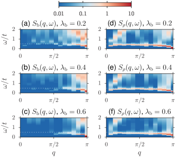
Figure 7: (a)–(c) Dynamic bond structure factor and (d)–(f) dynamic charge structure factor for $\lambda_{\text{s}}=0.3$, $L=30$.

For a stronger site coupling $\lambda_{\text{s}}=0.3$, the system undergoes a transition from the CDW Peierls phase to the BOW Peierls phase with increasing $\lambda_{\text{b}}$. The corresponding suppression (enhancement) of CDW (BOW) correlations was demonstrated in Fig. 4. Figure 6(d) suggests the absence of long-range BOW or CDW order at intermediate $\lambda_{\text{b}}=0.4$, and hence metallic behavior. The value $\lambda_{\text{b}}=0.4$ matches the position of the maximum in $K_{\rho/\sigma}(L)$ in Figs. 6(e)–(f), near which we also observe the crossover from dominant CDW to dominant BOW correlations. Furthermore, the single-particle gap is found to take on a minimum (not shown). The data for $K_{\rho}(L)$ in Fig. 6(e) appear to saturate near the maximum—a signature of a continuous phase transition with a closing of the charge gap [18]. In contrast, $K_{\sigma}(L)<1$ and $K_{\sigma}(L)\to 0$ for $L\to\infty$ [Fig. 6(f)] is consistent with a nonzero spin gap across the transition. These findings contrast the behavior across the Peierls-Mott transition in the Holstein-Hubbard model (at which all gaps close and $K_{\rho}=K_{\sigma}=1$ at the critical point [14; 15]) and in the SSH-Hubbard model (at which only the spin gap closes [8; 11]). The extended Hubbard model also exhibits CDW and BOW phases, but the intermediate Luther-Emery phase is restricted to a line [16; 17; 18; 19].

The transition from CDW to BOW order is further reflected in the renormalized phonon dispersions in Fig. 7. For weak coupling $\lambda_{\text{b}}=0.2$, the bond phonon mode is slightly renormalized [Fig. 7(a)] whereas the site phonon mode is soft [Fig. 7(d)]. At strong coupling $\lambda_{\text{b}}=0.6$, the bond mode is soft [Fig. 7(c)] while the site mode has hardened toward $\omega_{0}$ [Fig. 7(f)]. In between, Figs. 7(b) and (e), neither mode is soft, consistent with the absence of long-range order and metallic behavior.

Phase diagram.—While quantitative phase boundaries are beyond the scope of the present work, the schematic phase diagram of Fig. 1 was inferred from the following observations. Starting from $\lambda_{\text{s}}=0$, the metallic region is expected to grow because for a larger $\lambda_{\text{s}}$ the umklapp terms cancel at a larger $\lambda_{\text{b}}$. More physically, stronger CDW correlations require a larger $\lambda_{\text{b}}$ to be compensated before the BOW Peierls phase can emerge. An increase of the critical coupling is supported by a maximum in $K_{\rho/\sigma}(L)$ at larger $\lambda_{\text{b}}^{\text{max}}\approx 0.55$ for $\lambda_{\text{s}}=0.4$ as compared to $\lambda_{\text{b}}^{\text{max}}\approx 0.4$ for $\lambda_{\text{s}}=0.3$. Similarly, the CDW Peierls phase should appear at larger $\lambda_{\text{s}}$ for $\lambda_{\text{b}}>0$ due to the competing BOW correlations. Finally, the reduced extent of the metallic phase for $\lambda_{\text{s}}>\lambda_{\text{s}}^{c}$ was deduced from the observation of a sharper maximum in $K_{\rho}(L)$ for the same $L$ at $\lambda_{\text{s}}=0.4$ compared to $\lambda_{\text{s}}=0.3$. Whether there is a finite metallic phase or a metallic transition point in this regime has to be answered elsewhere.

Conclusions and outlook.—We studied a half-filled one-dimensional model of electrons coupled to site and bond quantum phonons by an exact quantum Monte Carlo method. The corresponding Holstein and SSH couplings favor different Peierls states. The results suggest that their competition provides a mechanism to restore the metallic behavior spuriously absent from the SSH model, in the form of a repulsive Luther-Emery phase with a spin gap. The transition between the two Peierls states appears to be continuous, and the Peierls gaps partially cancel each other. A physical picture is that of either bond or site spin singlets that are ordered in the Peierls phases but disordered in the metallic phase. While originally motivated by electron-phonon coupling in materials, the model also represents a generalization of extended Hubbard models to the case of retarded interactions, and describes the interplay of spin, charge and lattice fluctuations. Directions for future work include the exact phase diagram with its potential multicritical point, the impact of Mott physics driven by electron-electron repulsion, as well as competing interactions and finite-temperature phase transitions in two dimensions.