Photohadronic scenario in interpreting the February-March 2014 flare of 1ES 1011+496

Abstract

The extraordinary multi-TeV flare from 1ES 1011 +496 during February-March 2014 was observed by MAGIC telescopes for 17 nights and the average spectrum of the whole period has a non-trivial shape. We have used the photohadronic model and a template EBL model to explain the average spectrum which fits well to the flare data. The spectral index $\alpha$ is the only free parameter in our model. We have also shown that the non-trivial nature of the spectrum is due to the change in the behavior of the optical depth above $\sim 600$ GeV $\gamma$-ray energy accompanied with the high SSC flux.

I Introduction

The 1ES 1011+496 (RA: $153.767^{\circ}$, DEC: $49.434^{\circ}$) is a high frequency peaked BL Lac (HBL) object at a redshift of z= 0.212. This HBL was discovered at very high energy (VHE) $>$ 100 GeV by the MAGIC telescope in 2007 following an optical high state reported by the Tuorla Blazar Monitoring ProgramAlbert:2007kw . Two more multi-wavelength observations of the HBL were carried out by MAGIC in 2008Ahnen:2016hsc and in 2011-12Aleksic:2016wfj . During these two observation periods the source did not show any flux variability. On 5th February 2014, the VERITAS collaborationWeekes:2001pd issued an alert about the flaring of 1ES 1011+496 which was immediately followed by MAGIC telescopes from February 6th to March 7th, a total of 17 nightsAhnen:2016gog . The flare was observed in the energy range $\sim$ 75 GeV-3100 GeV and the flux could reach more than 10 times higher than any previously recorded flaring state of the sourceAlbert:2007kw ; Reinthal:2012gz . Despite this large variation, no significant intra-night variability was observed in the flux. This allowed the collaboration to use the average of the 17 nights observed spectral energy distribution (SED) to look for the imprint of the extragalactic background light (EBL) induced $\gamma$-rays absorption on itAhnen:2016gog .

The light produced from all the sources in the universe throughout the cosmic history pervades the intergalactic space which is now at longer wavelengths due to the expansion of the Universe and absorption/re-emission by dust and the light in the band 0.1–100 ${\mu}$m is called the diffuse EBLHauser:2001xs . The observed VHE spectrum of the distant sources are attenuated by EBL producing $e^{+}e^{-}$ pairs. While the EBL is problematic for the study of high redshift VHE $\gamma$-ray sources, at the same time the observed VHE $\gamma$-rays also provides an indirect method to probe the EBL. The relation between the intrinsic VHE flux $F_{\gamma,int}$ and the observed one $F_{\gamma,obs}$ are related throughHauser:2001xs ; Dominguez:2010bv

$$F_{\gamma,obs}(E_{\gamma})=F_{\gamma,int}(E_{\gamma})\,e^{-\tau_{\gamma\gamma}(E_{\gamma},z)},$$ (1)

where $\tau_{\gamma\gamma}$ is the optical depth. As the HBL 1ES 1011+496 is at a intermediate redshift, the observation of the VHE flare from it will provide a good opportunity to study the EBL effect. Although a large number of different EBL models existStecker:1992wi ; Salamon:1997ac ; Franceschini:2008tp ; Dominguez:2010bv ; Dominguez:2013lfa , here we shall discuss two important models by Franceschini et al. Franceschini:2008tp and Dominguez et al.Dominguez:2010bv ; Dominguez:2013lfa , which are used by Imaging Atmospheric Cherenkov Telescopes (IACTs) to study the EBL effect on the propagation of high energy $\gamma$-rays.

The SEDs of the HBLs have a double peak structure in the $\nu-\nu F_{\nu}$ plane. While the low energy peak corresponds to the synchrotron radiation from a population of relativistic electrons in the jet, the high energy peak believed to be due to the synchrotron self Compton (SSC) scattering of the high energy electrons with their self-produced synchrotron photons. The so called leptonic model which incorporates both the synchrotron and SSC processes in it is very successful in explaining the multi-wavelength emission from blazars and FR I galaxiesFossati:1998zn ; Ghisellini:1998it ; Abdo:2010fk ; Roustazadeh:2011zz ; Dermer:1993cz ; Sikora:1994zb . However, difficulties arise in explaining the multi-TeV emission detected from many flaring AGNAharonian:2009xn ; Abramowski:2011ze ; Krawczynski:2003fq ; Cui:2004wi ; Blazejowski:2005ih which shows that leptonic model may not be efficient in multi-TeV regime.

II Photohadronic Model

We employ photohadronic model to explain the multi-TeV flaring from many HBLsMucke:1998mk ; Mucke:2000rn ; Sahu:2013ixa ; Sahu:2013cja ; Sahu:2015tua . Here the standard interpretation of the leptonic model is used to explain the low energy peaks. Thereafter, it is proposed that the low energy tail of the SSC photons in the blazar jet serve as the target for the Fermi-accelerated high energy protons, within the jet to produce TeV photons through the decay of $\pi^{0}$s from the $\Delta$-resonanceSahu:2013ixa . But the efficiency of the photohadronic process depends on the photon density in the blazar jet. In a normal jet, the photon density is low which makes the process inefficient. However, during the flaring, it is assumed that the photon density in the inner jet region can go up so that the $\Delta$-resonance production is moderately efficient. Here, the flaring occurs within a compact and confined volume of radius $R^{\prime}_{f}$ (quantity with ^′ implies in the jet comoving frame) inside the blob of radius $R^{\prime}_{b}$ ($R^{\prime}_{f}<R^{\prime}_{b}$). The bulk Lorentz factor in the inner jet should be larger than the outer jet. But for simplicity we assume $\Gamma_{out}\simeq\Gamma_{in}\simeq\Gamma$. We cannot estimate the photon density in the inner jet region directly as it is hidden. For simplicity, we assume the scaling behavior of the photon densities in different background energies as followsSahu:2013ixa ; Sahu:2013cja ; Sahu:2015tua :

$${n^{\prime}_{\gamma,f}(\epsilon^{\prime}_{\gamma_{1}})}{n^{\prime-1}_{\gamma,f}(\epsilon^{\prime}_{\gamma_{2}})}\simeq{n^{\prime}_{\gamma}(\epsilon^{\prime}_{\gamma_{1}})}{n^{\prime-1}_{\gamma}(\epsilon^{\prime}_{\gamma_{2}})}.$$ (2)

Above equation implies that the ratio of photon densities at two different background energies $\epsilon^{\prime}_{\gamma_{1}}$ and $\epsilon^{\prime}_{\gamma_{2}}$ in the flaring state ($n^{\prime}_{\gamma,f}$) and in the non-flaring state ($n^{\prime}_{\gamma}$) remain almost the same. The photon density in the outer region is calculated from the observed flux in the usual way. So the unknown internal photon density is expressed in terms of the known photon density calculated from the observed/fitted SED in the SSC region which is again related to the observed flux in the same region. This model explains very nicely the observed TeV flux from the orphan flares of 1ES1959+650, Markarian 421 as well as multi-TeV flaring from M87Sahu:2013ixa ; Sahu:2013cja ; Sahu:2015tua .

In the observer frame, the $\pi^{0}$-decay photon energy $E_{\gamma}$ and the background SSC photon energy $\epsilon_{\gamma}$ are related through,

$$E_{\gamma}\epsilon_{\gamma}\simeq 0.032\,{\cal D}^{2}\,(1+z)^{-2}~{}{\rm GeV}^{2},$$ (3)

where $E_{\gamma}$ satisfy the relation $E_{p}=10\Gamma{\cal D}^{-1}E_{\gamma}$. ${\cal D}\simeq\Gamma$ is the Doppler factor of the relativistic jet and $E_{p}$ is the observed proton energy. The intrinsic flux $F_{\gamma,int}$ of the flaring blazar is proportional to a power-law with an exponential cut-off given as $E^{-\alpha}_{\gamma}\,e^{-E_{\gamma}/E_{\gamma,c}}$, with the spectral index $\alpha\geq 2$ and the cut-off energy is $E_{\gamma,c}$Aharonian:2003be . The effect of both the exponential cut-off and the EBL contribution are to reduce the VHE flux. For far-off sources the EBL plays the dominant role which shows that the $E_{\gamma,c}$ is much higher than the highest energy $\gamma$-ray observed during the VHE flaring event. Including EBL effect in the photohadronic scenarioSahu:2015tua the observed multi-TeV flux is expressed as

$$F_{\gamma,obs}(E_{\gamma})=A_{\gamma}\Phi_{SSC}(\epsilon_{\gamma})E^{-\alpha+3}_{\gamma,GeV}\,e^{-\tau_{\gamma\gamma}(E_{\gamma},z)}.$$ (4)

The SSC energy $\epsilon_{\gamma}$ and the observed energy $E_{\gamma}$ satisfy the condition given in Eq. (3), $\Phi_{SSC}(\epsilon_{\gamma})$ is the SSC flux corresponding to the energy $\epsilon_{\gamma}$ and $E_{\gamma,GeV}$ implies $E_{\gamma}$ expressed in units of GeV and $A_{\gamma}$ is the dimensionless normalization constant calculated from the observed flare dataSahu:2015tua . The spectral index $\alpha$ is the only free parameter here. By comparing Eqs. (1) and (4) $F_{\gamma,int}$ can be obtained.

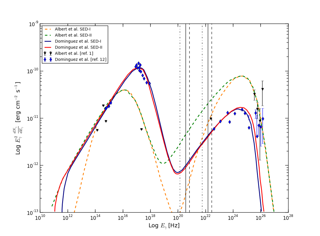
Figure 1: The leptonic SED of the HBL 1ES 1011+496 is shown by using two different models Albert et al. and Dominguez et al. Each of these models has two different parametrization which we call as SED-I and SED-II. Also the regions in the SED where the VHE protons interact with the SSC photons to produce the multi-TeV flare are shown: region between the two dashed dotted vertical lines corresponds to SED-II of Dominguez et al. with ${\cal D}=9.1$, region between the two vertical lines corresponds to SED-I of Dominguez et al. with ${\cal D}=14.6$ and the region between the two vertical dashed lines corresponds to SED-I, II of Albert et al. with ${\cal D}=20$.

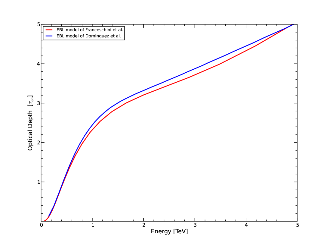
Figure 2: At a redshift of $z=0.212$, the optical depth $\tau_{\gamma\gamma}$ in the EBL models of Dominguez et al. and Franceschini et al. are shown for comparison.

III Results

The MAGIC collaboration fitted the average of the 17 nights observed SEDs of HBL 1ES 1011+496 with several functions, however, non of these fit well due to the non-trivial nature in the VHE limit. Also the intrinsic SED is calculated by subtracting the EBL contribution from the observed flux and is fitted with a simple power-law. We use the photohadronic scenario to interpret this flaring. The input for the photohadronic process comes from the leptonic model i.e. $\Gamma$, $\Phi_{SSC}$, and magnetic field etc. We come across two different leptonic models by Albert et al.Albert:2007kw and Dominguez et al. Dominguez:2013lfa which explain the low energy SED of the HBL 1ES 1011+496 and each of them has two different parametrization to fit the observed data as shown in Fig. 1. In Dominguez et al. model, the two different SEDs have almost the same flux in the SSC energy range. So we only consider one of the SEDs (SED-II) here.

The EBL models of Dominguez et al. and Franceschini et al., are widely used to constraint the imprint of EBL on the propagation of VHE $\gamma$-rays by IACTs . We compared $\tau_{\gamma\gamma}$ of both these models (the central value of the former model is used) for $E_{\gamma}<5$ TeV and found a very small difference as shown in Fig. 2. So for our analysis here we only consider the Dominguez et al. model. However, the results will be similar for the other one . There are three distinct regions of $E_{\gamma}$ in Fig. 2, where the behavior of $\tau_{\gamma\gamma}$ is different. Below $E_{\gamma}\sim 600$ GeV it has a rapid growth. In the energy range $\sim 600$ GeV to $\sim 1.2$ TeV the growth is slow and above $\sim 1.2$ TeV the growth is almost linear. This growth pattern of $\tau_{\gamma\gamma}$ influences the $F_{\gamma,obs}$ in different models and the results of the above two leptonic models are discussed separately.

III.1 Leptonic model of Albert et al.Albert:2007kw

Here the SED is modeled by using the single zone synchrotron-SSC model where the emission region is a spherical blob of radius $R^{\prime}_{b}\sim 10^{16}$ cm and a Doppler factor ${\cal D}=20$ is taken. The emission region has a magnetic field $B^{\prime}\sim 0.15$ G and the relativistic electrons emit synchrotron radiation which explain the low energy peak of the SED. The high energy emission from X-rays to few GeV $\gamma$-rays are from the Compton scattering of the seed synchrotron photons by the same population of high energy electrons. Here two different SEDs are considered to fit the low energy data. In the hadronic model alluded to previously, $75.6\,GeV\leq E_{\gamma}\leq 3.1\,TeV$ corresponds to the Fermi accelerated proton energy in the range $0.76\,TeV\leq E_{p}\leq 31\,TeV$ which collide with the SSC photons in the inner jet region in the energy range $115\,MeV\,(2.8\times 10^{22}\,Hz)\geq\epsilon_{\gamma}\geq 2.8\,MeV\,(6.8\times 10^{20}\,Hz)$ to produce the $\Delta$-resonance and its decay to $\pi^{0}$s produces observed multi-TeV $\gamma$-rays. Using the scaling behavior of Eq. (2), photon densities in the inner and outer regions of the jet can be related. In the outer region, the above range of $\epsilon_{\gamma}$ corresponds to the low energy tail of the SSC photons (energy range between two dashed vertical lines in Fig. 1). We observe that the $\Phi_{SSC}$ for SED-II is always larger than the corresponding flux of SED-I. As we know from Eq. (4), $F_{\gamma,obs}$ is proportional to $\Phi_{SSC}$, so with the inclusion of EBL contribution, the calculated $F_{\gamma,obs}$ with SED-II is always $\geq$ the flux with SED-I in the above range of $\epsilon_{\gamma}$.

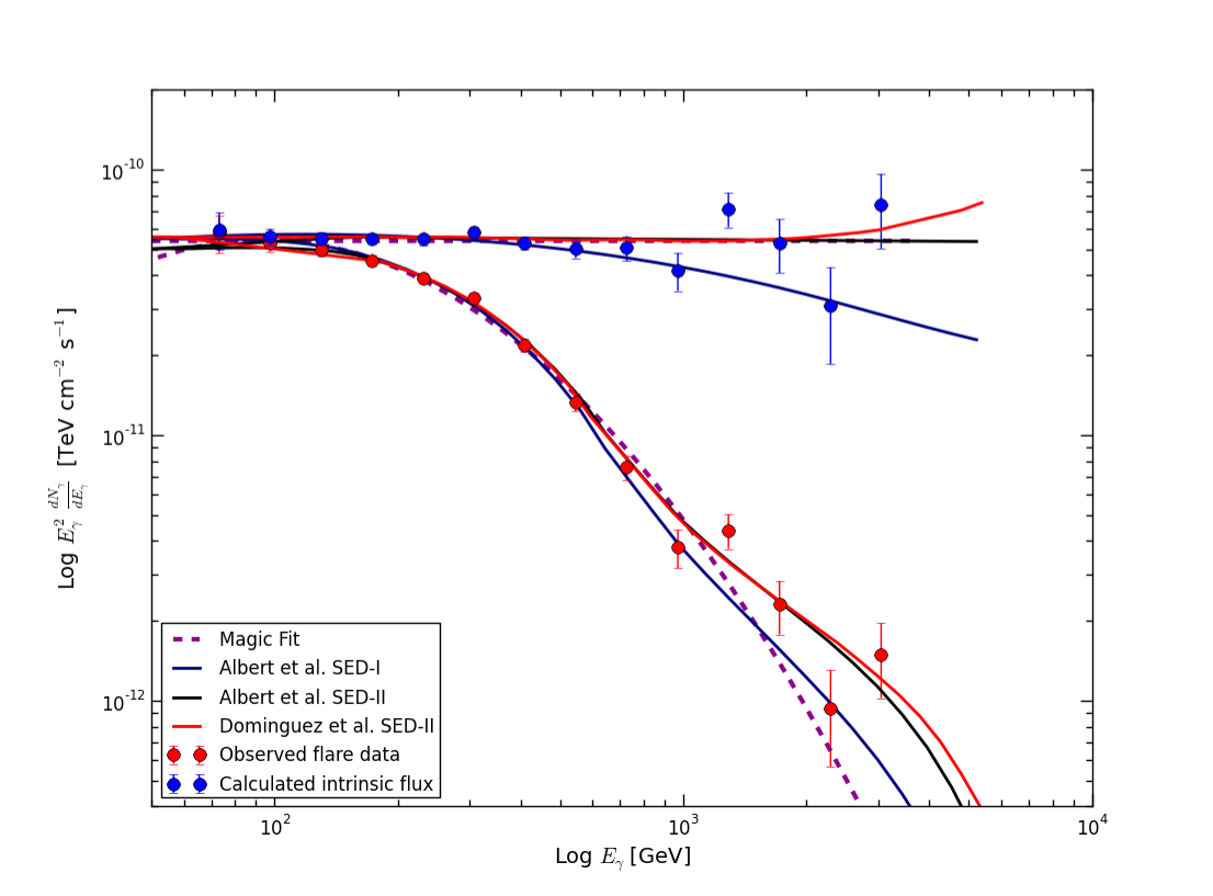
Figure 3: Using leptonic models of Albert et al. and Dominguez et al. and the EBL correction, the multi-TeV flare data are fitted in the photohadronic model (lower curves) and the corresponding intrinsic fluxes are also shown (upper curves). The lower and the upper curves of same color belong to a single model. For comparison the MAGIC fit to the observed flux (lower magenta dashed curve) and the intrinsic flux (upper magenta dashed curve) are shown.

The $F_{\gamma,obs}$ and $F_{\gamma,int}$ for SED-I are plotted as functions of $E_{\gamma}$ in Fig. 3. A good fit to flare data is obtained for the normalization constant $A_{\gamma}=0.37$ and the spectral index $\alpha=2.3$ (blue curves). Our model fits very well with the flare data up to energy $E_{\gamma}\sim 1$ TeV and above this energy the flux falls faster than the observed data. Above 500 GeV the $F_{\gamma,int}$ (upper blue curve) falls faster than the MAGIC fit which is a constant. This fall in $F_{\gamma,int}$ is also responsible for the faster fall in $F_{\gamma,obs}$ in the energy range $\sim 500$ GeV to 1.2 TeV even if the fall in $e^{-\tau_{\gamma\gamma}}$ is slow. Above $E_{\gamma}\sim 1.2$ TeV, the linear growth in $\tau_{\gamma\gamma}$ wins over the fall in $F_{\gamma,int}$ so that the fall in $F_{\gamma,obs}$ is slowed down. For comparison we have also shown the log-parabola fit by MAGIC collaboration (lower magenta dashed curve), however, both these fits are poor in VHE limit.

We have also plotted $F_{\gamma,obs}$ and $F_{\gamma,int}$ for SED-II. Here a good fit is obtained for $A_{\gamma}=0.64$ and $\alpha=2.6$ (lower black curve). We observed that the MAGIC fit to $F_{\gamma,int}$ and our result (upper black curve) are the same and constant in all the energy range. In the photohadronic model, above $\sim 1$ TeV the $F_{\gamma,obs}$ has a slow fall even though the $F_{\gamma,int}$ is constant for all energies. Again the curve changes its behavior above $\sim 1.2$ TeV. This peculiar behavior is due the slow growth of $\tau_{\gamma\gamma}$ in the range $600\,GeV\leq E_{\gamma}\sim 1.2$ TeV and above this energy almost a linear growth. The comparison of $F_{\gamma,obs}$ in SED-I and SED-II shows a marked difference for $E_{\gamma}>0.8$ TeV. The lower black curve (SED-II) falls slower than the lower blue curve (SED-I) . The higher value of $\Phi_{SSC}$ in SED-II compared to the one in SED-I in the energy range $115\,MeV\geq\epsilon_{\gamma}\geq 2.8\,MeV$ is responsible for this discrepancy which can be seen from Fig. 1.

III.2 Leptonic model of Dominguez et al.Dominguez:2013lfa

As discussed above, this model uses two different parameterizations to fit the leptonic SED which we call as SED-I and SED-II as shown in Fig. 1. The SEDs obtained in both these cases are almost the same in the SSC energy range. So here we only consider SED-II. However, for SED-I the results will be very similar. The SED-II is fitted by considering the spherical blob of size $R^{\prime}_{b}=2.2\times 10^{16}$ cm moving with a bulk Lorentz factor $\Gamma=9.1$. A constant magnetic field $B^{\prime}\sim 0.23$ G is present in the blob region where the charged particles undergo synchrotron emission.

In the photohadronic scenario, the flare energy range $75.6\,GeV\leq E_{\gamma}\leq 3.1\,TeV$ corresponds to $23.9\,MeV\,(5.8\times 10^{21}\,Hz)\geq\epsilon_{\gamma}\geq 0.58\,MeV\,(1.4\times 10^{20}\,Hz)$ and the VHE proton energy in the range $0.76\,TeV\leq E_{p}\leq 31\,TeV$. The above range of $\epsilon_{\gamma}$ lies in the tail region of the SSC spectrum as shown in Fig. 1. In Fig. 3 we have also shown $F_{\gamma,obs}$ and $F_{\gamma,int}$ for SED-II. A good fit to flare data is obtained by taking $A_{\gamma}=5.9$ and $\alpha=2.6$ (lower red curve). We observed that our model fit decreases slower than the MAGIC fit and model fits of Albert et al. above $\sim 1$ TeV. The comparison of $F_{\gamma,int}$ (upper red curve) with the MAGIC fit shows that both are practically the same for $E_{\gamma}<2$ TeV and above this energy the photohadronic prediction increases slightly, however, there is a big difference in $F_{\gamma,obs}$ above $E_{\gamma}>1$ TeV. From Eq. (4) we observed that both the intrinsic and the observed fluxes are proportional to $E^{-\alpha}_{\gamma}$ and are independent of an exponential cut-off. However, if at all there is a cut-off energy it must be $E_{\gamma,c}\geq 70$ TeV, otherwise the $F_{\gamma,obs}$ will fall faster than the predicted fluxes shown in black and red lower curves in Fig. 3 which will be non compatible with the flare data.

IV Conclusions

The multi-TeV flaring of February-March 2014 from 1ES 1011+496 is interpreted using the photohadronic scenario. To account for the effect of the diffuse radiation background on the VHE $\gamma$-rays we incorporate a template EBL model to calculate the observed flux. Also two different leptonic models are considered to fit the flare data and the results are compared. The spectral index $\alpha$ is the only free parameter here. The flare data has a non-trivial shape above $E_{\gamma}\sim 600$ GeV and in photohadronic model this behavior can be explained by the slow to linear growth in $\tau_{\gamma\gamma}$ above this energy range complemented by higher SSC flux. The EBL contribution alone cannot explain the non-trivial shape of the data which can be clearly seen by comparing the lower blue curve with the lower black and red curves in Fig. 3. Towards the end of the observation period by the MAGIC telescopes, the source activity was lower which amounted to larger uncertainties in the flux and correspondingly the average spectrum. Probably this might be the reason for larger uncertainties in the VHE range of the average spectrum. The MAGIC telescopes exposure period for most of the nights was $\sim 40$ minutes which was extended for $\sim 2$ hours on nights of 8th and 9th FebruaryAhnen:2016gog . This extended period of observation might have better flux resolution and our expectation is that photohadronic scenario will be able to fit the data well. In future, for a better understanding of the EBL effect and the role played by the SSC photons on the VHE $\gamma$-ray flux from intermediate to high redshift blazars, it is necessary to have simultaneous observations in multi-wavelength to the flaring objects.

We thank Adiv Gonzalez and Lucy Fortson for many useful discussions. The work of S. S. is partially supported by DGAPA-UNAM (Mexico) Project No. IN110815.

References

- (1) J. Albert et al. [MAGIC Collaboration], Astrophys. J. 667, L21 (2007).
- (2) M. L. Ahnen et al. [MAGIC and AGILE Collaborations], Mon. Not. Roy. Astron. Soc. 459, 2286 (2016).
- (3) J. Aleksić, et al., Astron. Astrophys. 591, A10 (2016).
- (4) T. C. Weekes et al., Astropart. Phys. 17, 221 (2002).
- (5) M. L. Ahnen et al., Astron. Astrophys. 590, A24 (2016).
- (6) R. Reinthal et al. [MAGIC and AGILE Team Collaborations], J. Phys. Conf. Ser. 355, 012017 (2012).
- (7) M. G. Hauser and E. Dwek, Ann. Rev. Astron. Astrophys. 39, 249 (2001).
- (8) A. Dominguez et al., Mon. Not. Roy. Astron. Soc. 410, 2556 (2011).
- (9) M. H. Salamon and F. W. Stecker, Astrophys. J. 493, 547 (1998).
- (10) F. W. Stecker, O. C. de Jager and M. H. Salamon, Astrophys. J. 390, L49 (1992).
- (11) A. Franceschini, G. Rodighiero and M. Vaccari, Astron. Astrophys. 487, 837 (2008).
- (12) A. Dominguez, J. D. Finke, F. Prada, J. R. Primack, F. S. Kitaura, B. Siana and D. Paneque, Astrophys. J. 770, 77 (2013).
- (13) A. A. Abdo et al. [Fermi LAT Collaboration], Astrophys. J. 719, 1433-1444 (2010).
- (14) P. Roustazadeh and M. Böttcher, Astrophys. J. 728, 134 (2011).
- (15) G. Fossati, L. Maraschi, A. Celotti, A. Comastri and G. Ghisellini, Mon. Not. Roy. Astron. Soc. 299 (1998) 433.
- (16) G. Ghisellini, A. Celotti, G. Fossati, L. Maraschi and A. Comastri, Mon. Not. Roy. Astron. Soc. 301 (1998) 451.
- (17) C. D. Dermer and R. Schlickeiser, Astrophys. J. 416, 458 (1993).
- (18) M. Sikora, M. C. Begelman and M. J. Rees, Astrophys. J. 421, 153 (1994).
- (19) F. Aharonian et al. [HESS Collaboration], Astrophys. J. 695, L40 (2009).
- (20) A. Abramowski et al. [H.E.S.S. and VERITAS Collaborations], Astrophys. J. 746, 151 (2012).
- (21) H. Krawczynski, S. B. Hughes, D. Horan, F. Aharonian, M. F. Aller, H. Aller, P. Boltwood and J. Buckley et al., Astrophys. J. 601, 151 (2004).
- (22) W. Cui et al. [VERITAS Collaboration], AIP Conf. Proc. 745, 455 (2005).
- (23) M. Blazejowski, G. Blaylock, I. H. Bond, S. M. Bradbury, J. H. Buckley, D. A. Carter-Lewis, O. Celik and P. Cogan et al., Astrophys. J. 630, 130 (2005).
- (24) A. Mucke, J. P. Rachen, R. Engel, R. J. Protheroe and T. Stanev, Publ. Astron. Soc. Austral. 16, 160 (1999).
- (25) A. Mucke and R. J. Protheroe, Astropart. Phys. 15, 121 (2001).
- (26) S. Sahu, A. F. O. Oliveros and J. C. Sanabria, Phys. Rev. D 87, 103015 (2013).
- (27) S. Sahu, L. S. Miranda and S. Rajpoot, Eur. Phys. J. C 76, 127 (2016).
- (28) S. Sahu and E. Palacios, Eur. Phys. J. C 75, 52 (2015).
- (29) F. Aharonian et al. [HEGRA Collaboration], Astron. Astrophys. 406, L9 (2003).