Binary classification of multi-channel EEG records based on the $\epsilon$-complexity of continuous vector functions

Abstract

A methodology for binary classification of EEG records which correspond to different mental states is proposed. This model-free methodology is based on our theory of the $\epsilon$-complexity of continuous functions which is extended here (see Appendix) to the case of vector functions. This extension permits us to handle multichannel EEG recordings. The essence of the methodology is to use the $\epsilon$-complexity coefficients as features to classify (using well known classifiers) different types of vector functions representing EEG-records corresponding to different types of mental states. We apply our methodology to the problem of classification of multichannel EEG-records related to a group of healthy adolescents and a group of adolescents with schizophrenia. We found that our methodology permits accurate classification of the data in the four-dimensional feather space of the $\epsilon$-complexity coefficients.

Introduction

An electroencephalogram (EEG) is a direct measure of electrical activities of the brain along the scalp. It is a rich source of information about the brain for healthy individuals and patients with neurological diseases. Compared to the blood flow neuroimaging techniques, such as magnetic resonance imaging (MRI) and functional magnetic resonance imaging (fMRI), which are indirect measures of brain activity, EEG is cheaper and easier to use. An additional strength of EEG is that it can detect changes within a millisecond time frame whereas fMRI has time resolution between seconds and minutes. Quantitative evaluation of cognitive functioning and mental states using EEG records is one of the important problems in applied psychophysiology [1]. They include brain-computer interface [2, 3, 4] for decoding intentions and their translation into commands, and diagnosis of mental illnesses such as schizophrenia [1, 5, 6].

To obtain useful information from the EEG data feature extraction is necessary. In the literature a whole set of quantitative estimates of the spectral and temporal features of the EEG signal have been developed (see, e.g. [7]). In particular, there is an extensive literature on attempts to use these characteristics for schizophrenia diagnosis (for review and meta-analysis of such papers see e.g. [8]). However such approach requires assumptions on a data generating mechanism but there are no generally excepted model on the data generated mechanism for EEG data.

Another approach to select features is related to the fundamental concepts of the modern theory of nonlinear dynamical systems such as entropy, correlation dimension $D_{2}$ and Lyapunov exponent (see, e.g. [9, 10, 11, 12]). These features can really reflect the complexity of a generating mechanism of a signal, but only under the assumptions of stationarity and ergodicity of a signal. Due to the nature of EEG signals these assumptions are not fully justifiable (see, e.g. [13, 14]).

To the best of our knowledge the papers which produce a high accuracy on classification of EEG signal use high-dimensional feature space and face the problem of overfitting (see e.g. [15])

In this paper we propose an approach to the feature selection problem which is model free (e.g. does not have any assumptions on data generating mechanism such as stationarity or ergodicity of the data). It also assures a good accuracy in small dimensional feature space. More precisely, we propose to apply the notion of the $\epsilon$-complexity of continuous functions to the classification problem of multichannel EEG-records. Such approach is in line with general Kolmogorov’s idea on a ‘‘complexity’’ of an object. At the basic level the idea of a Kolmogorov can be expressed as follows: A ‘‘complex’’ object requires a lot of information for its reconstruction and, for a ‘‘simple’’ object, little information is needed. Therefore, it is quite natural to measure the complexity of a continuous function by the number of function values on a uniform grid (e.g. function values given at equally distant points) which are necessary to reconstruct the function with a given error by a given set of methods. This characteristic of complexity was tested on evaluation of the functional states of the brain using the EEG recordings in [16, 18]. It was found that the mean values of complexity are statistically significantly different for the groups of subjects with different functional states. This result was obtained despite the fact that the easiest method of function reconstruction by piecewise-constant approximation was used. However, for further progress in this area the development of computational procedure for estimation of the ‘‘complexity’’ of an individual recording (i.e. an individual continuous function) was required. This was impossible without development of an appropriate mathematical theory.

In 2012-2014 ( see, [darkhovsky2012new, 19, 20, 21]) the theory of the $\epsilon$-complexity of continuous functions defined on a compact set in a finite-dimensional space was developed. It was proven that the $\epsilon$-complexity of ‘‘almost all’’ Hölder functions is effectively characterized by a pair of real numbers, which we call the $\epsilon$-complexity coefficients. This theory enabled us to develop a novel approach to the problems of segmentation and classification of time series of arbitrary nature. In this paper we extended the theory of the $\epsilon$-complexity of continuous functions to the case of continuous vector-functions (see Appendix). This extension enables us to apply such approach to the binary classification problem of EEG records.

The paper is organized as follows. In Section 1 we describe our methodology. In particular, in Subsection 1.1 we give a description of the notion of the $\epsilon$-complexity of a vector function on a semantic level and provide a characterization of the $\epsilon$-complexity for vector functions given by a finite set of values. In Subsection 1.2 we provide an algorithm for estimation of the $\epsilon$-complexity coefficients for the multichannel EEG records. In Subsection 1.3 we describe our classification procedure. In Section 2 we apply our methodology to the classification of the EEG records of adolescents with schizophrenic type of disorder and of healthy subjects. We have established that these data permit accurate classification in the four-dimensional space of the $\epsilon$-complexity coefficients of original EEG signals and $\epsilon$-complexity coefficients of fourth differences of EEG signals. In Section 3 we provide conclusions and discuss our results. The Appendix provides the precise definition of $\epsilon$-complexity and the theorem characterizing the complexity of Hölder vector functions

1 Methodology

In this section, we give a description of proposed methodology for classification of multi-channel EEG-records.

We will treat a multichannel EEG record as a $d$-dimensional vector function $x(t)=\left(x_{1}(t),\dots,x_{d}(t)\right)$, where $d$ is a number of channels, which is given on some fixed time interval $t\in[0,T]$ .

Since the modern recording equipment is digital, instead of a continuous vector function $x(t)$ the researcher received a discrete samples $\left(x(0),x(T/n),x(2T/n),\dots,x(T)\right)$, e.g. , the sequence of $n$ $d$-dimensional vectors. Here $n=fT$, where $f$ is a sample frequency (if the frequency is measured in Hz, e.g. time in seconds). For example, if $T=60$ seconds, and $f=128$Hz, then we have 7680 $d$-dimensional vectors.

Without loss of generality we can assume that $\max\limits_{0\leq k\leq n}|x_{i}(kT/n)|=R_{i}>0,\,i=1,2,\dots,d$, e.g. in each channel of EEG signal is present.

1.1 Description of the $\epsilon$-complexity of continuous vector function

Let us describe our notion of the $\epsilon$-complexity on semantic level. The precise definition and formulation of the theorem are given in Appendix.

We choose a number $0<S<1$ and discard from each component of a vector function $\{x_{i}(kT/n)\}_{k=0}^{k=n},\,i=1,\dots,d$ $[(1-S)n]$ values (henceforth, the symbol $[a]$ denotes the integral part of a number $a$), in such a way that the remaining values are approximately uniformly distributed. For example, if $S=0.5$, then we retain even or odds values in each component of the function.

Assume we have some fixed collection $\mathcal{F}$ of approximation methods which can be used for reconstruction of a continuous function by its values at some uniform grid. Employing collection of methods $\mathcal{F}$, we reconstruct the values of each component of the vector function $i,\,i=1,\dots,d$ in discarded points using the retained values of the function. We find the methods which reconstruct the function with minimum relative (in relation to $R_{i},i=1,\dots,d$) error (the error can be measured in any norm, because we are dealing with a finite a set of values).

Denote the value of the minimum relative reconstruction error in the $i$-th component through $\epsilon_{i}(S)$ and find the value $\epsilon(S)=\sum\limits_{i=1}^{d}\epsilon_{i}(S)$.

Now we will define the $(\epsilon,\mathcal{F})$-complexity (hereafter, for simplicity of presentation we will write $\epsilon$-complexity) of continuous vector function $x(t)$, which is given by its values on the uniform grid by $(-\log S)$.

In other words, the $\epsilon$-complexity of a vector function is the (minus) logarithm of relative fraction of their values, required for its recovery by methods from family $\mathcal{F}$ with a relative error no more than $\epsilon$. In other words, it is ‘‘the shortest’’ description of the vector function.

Let us consider the class of vector functions satisfying the Hölder condition. It means that for any $(t,s)\in[0,T]\times[0,T]$ the following inequality holds

$$\sum\limits_{i=1}^{d}|x_{i}(t)-x_{i}(s)|\leq L|t-s|^{p},\,\,L>0,p>0.$$ (1)

This class of vector functions is very wide, and it includes practically all vector functions which can be found in applications.

The main point of our classification methodology is as follows. For ‘‘almost all’’ vector functions satisfying the Hölder condition, in case of sufficiently rich family $\mathcal{F}$ of approximation methods and a sufficiently large sample size $n$ there exists range $0<\alpha(n)\leq S\leq\beta(n)<1$ (which depends from vector function) such that the following equality holds

$$\log\epsilon\approx A+B\log S$$ (2)

The precise meaning of the expression ‘‘almost any’’ and symbol $\approx$ will be explained in the Appendix.

The above parameters $A,B$ are called the $\epsilon$-complexity coefficients. These $\epsilon$-complexity coefficients will be utilized as features for classification of multichannel EEG records. In our work we will use supervised classifiers such as random forest and support vector machine.

These features don’t depend from the data generating mechanism and therefore they are model-free. In the scalar case they have been introduced and applied for the purpose to detect changes in generating mechanism [darkhovsky2012new, 19, 20, 21].

We would like to mention two facts. Firstly, in practical applications the family of function reconstruction methods $\mathcal{F}$ is finite. It follows from our main theorem (see Appendix) that if this family $\mathcal{F}$ is reach enough and the sample size of function values is large enough then the error of vector function reconstruction in discarded points by methods from this family (and therefore the $\epsilon$-complexity) is closed to the error of the reconstruction by all (computable ) methods.

Our experience with simulations and real data shows that the dependence (2) has been observed in case we chose piece-wise polynomial functions up to fourth degree as family $\mathcal{F}$.

Secondly, it is not significant which method gives the smallest error of reconstruction $\epsilon_{i}(S)$ in $i$-th channel ($i=1,\dots,d$). To find dependence (2) we need only values of minimal errors.

1.2 Algorithm for estimation of the $\epsilon$-complexity coefficients

In this subsection we will describe main steps of our algorithm for estimation of the $\epsilon$-complexity coefficients for multichannel EEG records.

1. Normalize each component of the EEG record $x_{i}(t)$, i.e replace our original components of the multichannel record by $x_{i}(t)/\max_{t}(|x_{i}(t)|)$.

2. Select $S$, the fraction of the remaining points as follows: $S_{1}=50\%$, $S_{2}=33\%$, $S_{3}=29\%$, $S_{4}=25\%$, $S_{5}=22.5\%$, $S_{6}=20\%$.

3. For each fixed $S_{i}$ ($i=1,\dots,6$) and for each component of the multichannel record discard the values of the functions at points which are placed uniformly, or almost uniformly, according to the following scheme: Let $x_{i}^{1},x_{i}^{2}$,$x_{i}^{3},\dots,x_{i}^{n}$ be the values of a function on a grid.

   1. ${S}_{1}=50\%$: Values of $x_{i}^{2},x_{i}^{4},\dots,x_{i}^{2j},\dots;$ or $x_{i}^{1},x_{i}^{3},\dots,x_{i}^{2j+1},\dots;$ are discarded. Notice we have two different ways to discard function values;

   2. $S_{2}=33\%$ :Values of $x_{i}^{1},x_{i}^{4},x_{i}^{7},x_{i}^{10},\dots$; or $x_{i}^{2},x_{i}^{5},x_{i}^{8},x_{i}^{11},\dots;$ or $x_{i}^{3},x_{i}^{6},x_{i}^{9},x_{i}^{12},\dots;$ are discarded. We have three different placements of discarded values;

   3. $S_{4}=25\%$ : Values of $x_{i}^{1},x_{i}^{5},x_{i}^{9},x_{i}^{13},x_{i}^{17},\dots;$ or $x_{i}^{2},x_{i}^{6},x_{i}^{10},x_{i}^{14},x_{i}^{18},\dots$;
      or $x_{i}^{3},x_{i}^{7},x_{11},x_{15},x_{19},\dots;$ or $x_{4},x_{8},x_{12},x_{16},x_{20},\dots;$ are discarded. We have 4 different placements of discarded values;

   4. The procedures are similar in the case $S_{3}=29\%$, $S_{5}=22.5\%$ and $S_{6}=20\%$.

4. For each $S_{k}$ and for each of those placements we consider all possible reconstructions of the function by piecewise polynomials up to fourth degree and select the one which provides the minimal error of reconstruction. Record this value of the minimal error.

5. For the same $S_{k}$ we consider other placements of the retained points and repeat the procedure. Record the obtained minimal errors.

6. Then we take a mean of the recorded errors calculated over all placements for each channel of the EEG-record.

7. Take sum of the mean errors over all channels. It is our estimation of $\epsilon_{k}$ in the case of $S_{k}$.

8. Repeat the procedure for $k=1,\dots,6$.

9. Consider points $(\log(S_{k}),\log(\epsilon_{k}))$, and find the best linear fit

   $$\log\epsilon\approx A+B\log S$$ (3)

   using the least squares method.

Each graph in Fig 1 demonstrates the typical dependence of the form (2) for given EEG recording (the theoretical dependence is shown by a solid line, and the experimental points are shown by circles). The left plot corresponds to the normal subject and the right one to the patient with schizophrenia.

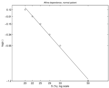
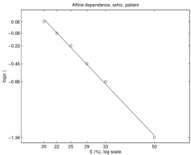
Figure 1: Typical dependencies of the form (3) of EEG recordings, left (A): normal subject, right (B): patient with schizophrenia. The theoretical dependence is shown by a solid line, and the experimental points are shown by circles.

Let us notice that the obtained above values of the coefficients $A$ and $B$ are our estimates for the $\epsilon$-complexity coefficients which are used in classification algorithm. For each subject we estimate the $\epsilon$-complexity coefficients as well as the $\epsilon$-complexity coefficients of some transformations of the EEG data (see next section).

1.3 Classification

In the next step we use the calculated $\epsilon$-complexity coefficients as an input to the supervised classifiers, such as Random Forest and Support Vector Machine. The results will be evaluated using the Out-Of-Bag (OOB) [22] error in case of the random forest and k-fold cross-validation procedure in both cases to be able to compare the performance of two classifiers.

Note that in case of OOB the model calculates the error using observations not trained for each decision tree in the forest and aggregates over all of them; therefore it has no bias. This is considered to be an accurate estimate of the test error for the Random Forest [22].

Cross-validation (CV), (see e.g,[23, 24] ) is a model validation technique for assessing how the results of a statistical analysis will be generalized to a new data set. In particular, the data set is partitioned into complementary subsets (so called training and validation sets). The classifier is built using the training data set and performance is tested on the validation set. In $k$-fold cross-validation (see, e.g [24, 25]), the original sample is randomly partitioned into $k$ equal-sized subsamples. Of the $k$ subsamples, a single subsample is retained as the validation data for testing the classifier, and the remaining $k-1$ subsamples are used as training data. The cross-validation process is then repeated $k$ times, with each of the $k$ subsamples used exactly once as the validation data. The $k$ results from the folds are averaged to produce a single estimate.

2 Results

Data description. EEG recordings which were analyzed previously in [26, 27, 28] are also used in this study. The data are publicly available at http://brain.bio.msu.ru/eeg_schizophrenia.htm. The recordings have been obtained for 45 boys (10-14 years old) suffering from schizophrenia and diagnosed using clinical interviews at the Research Center for Psychological Disorders of the Russian Academy of Medical Sciences according to the criteria given in [30]. Because the patients had not taken psychoactive drugs before participating in the study, we could exclude the influence of medications. The control group consists of 39 healthy boys (11-13 years old). The traditional approach to placement of electrodes used at Pirogov Russian National Research Medical University in similar studies was employed. For all subjects EEG were registered using the standard 10/20 international electrode scheme involving 16 electrodes (O1, O2, P3, P4, Pz, T5, T6, C3, C4, Cz, T3, T4, F3, F4, F7, F8) with the reference earlobe electrode.

Artifacts, mostly head and eyes movements, were removed manually based on the opinion of two experts. We received data which are free of the artifacts. During the recordings patients were in resting state with closed eyes. Impedance for all electrodes was kept below 10 k$\Omega$. Signal was sampled at frequency 128Hz and bandpass filter between 0.5Hz and 45Hz was applied. The length of each recording after removal of the artifacts is 7680 points.

Remark. The bandpass-filter between 0.5 and 45Hz was performed initially. We did not perform any additional filtration of the signal in different frequency bands. Note the filtration changes the signal and therefore, generally speaking its $\epsilon$-complexity. However in our attempt to classify the EEG signals into schizophrenic and control groups we did not have a preliminary information which frequency band can be used as classification feature. Therefore we did not perform such filtration and as it turned out later, we need not it.

In our analysis the multichannel EEG record is treated as a restriction of a continuous vector function $x(t)=\left(x_{1}(t),\dots,x_{16}(t)\right),t\in[a,b]$ at the uniform grid, i.e. values of continuous vector function are given in equally distant points of time with distance 1/128 sec.

For all individuals in our study we estimated the $\epsilon$-complexity coefficients $A_{i},B_{i}$ according to the above algorithm. Here, $i$ is the subject’s number, $i=1,\dots,84$, where the first 39 subjects are normal and the last 45 subjects are schizophrenic.

After that we consider differences of the original EEG signals, $x^{(1)}(t)=x(t+1)-x(t)$, $t=1,..,n-1$, $x^{(2)}(t)=x^{(1)}(t+1)-x^{(1)}(t)$ $t=1,....,n-2$, and etc. The $\epsilon$-complexity coefficients $ADk_{i},BDk_{i}$, $k=1,2,3,4$ are estimated up to the fourth difference.

The employment of differences corresponds to the analysis of derivatives of the EEG signal. Since, a priory , we did not know the features of the signal which are useful for classification, we tested different combinations of the $\epsilon$-complexity coefficients of the original series and the series of finite differences and found that the complexity coefficients $A_{i},B_{i}$, and complexity coefficients of 4th differences $AD4_{i},BD4_{i}$ ($i=1,\dots,84$) form the best set of features for classification of our patients into two groups: schizophrenic and control.

After that we use the machine learning techniques to separate data into two clusters. In particular, we feed the vectors $(A_{i},B_{i},AD4_{i},BD4_{i})$ into the supervised classifiers such as Random Forest (RF) and Support Vector Machine classifiers (SVM). This step is performed using R project software and its package "RandomForest" for the random forest classifier and package "e1071" for the SVM. We also perform 10-fold cross-validation using the "cart" package.

The results for the OOB and the $10$-fold cross-validation for Random Forest and SVM classifiers are presented in the Table 1. In this table we provide the accuracy of these classifiers and the percentage of false negative and false positive cases. False positive cases are the cases in which we classify the healthy patient as a patient with schizophrenia and false negative cases are the cases in which we classify a patient with schizophrenia as a healthy patient. To get 95% bootstrap confidence intervals (CI) we performed 10,000 replications of our experiments using random re-sampling of the data.

Table 1. (Results for the Random Forest (RF) and Support Vector Machine (SVM) classifiers)

Method		Accuracy (in $\%$)	False Positive (in $\%$)	False Negative (in $\%$)
RF	OOB	83.6	11.6	20.7
RF	95% CI	(80.9, 85.7)	(10.3, 15.4)	(17.8, 22.2)
RF	10-fold CV	83.2%	13.1%	21.5%
RF	95% CI	(79.2,86.8)	(7.5, 20.0)	(16.0,27.0)
SVM	10-fold CV	79.7%	13.6%	25.9%
SVM	95% bootstrap CI	(75.9,83.4)	(8.3, 19.2)	(20.5,31.7)

3 Conclusions and Discussion

Until now the problem of detecting EEG mental states in humans and in particular, in the diagnosis of mental diseases, remains open [7, 15]. This is due to the lack of effectiveness of traditional methods of EEG analysis in relation to the classification of normal and pathological mental states [badrakalimuthu2011eeg, 31] that causes the researchers to seek new methods of quantitative evaluation of the EEG including schizophrenia detection and classification [15].

In this paper, we proposed methodology which employs the $\epsilon$-complexity for the separation of different mental state. In particular, we apply this methodology to separate EEG records of patients with schizophrenia and control group.

We selected the multivariate $\epsilon$-complexity coefficients of the original data as well as the multivariate $\epsilon$-complexity coefficients of the fourth differences as markers in identification of schizophrenia in adolescents. We found that Random Forest classifier performs better for this data set than Support Vector Machine. The accuracy of proposed markers is relatively high, reaching on average $83.6\%$ in the test set used in the cross-validation on a sample of 45 schizophrenic patients and $39$ healthy subjects. The False Positive error rate on average is 11.6% and False Negative is 20.7%.

We would like to emphasize that the feature space used in classification algorithm has only four dimensions which is much smaller than the sample size. To the best of our knowledge, the literature does not contain any results on the classification of schizophrenic diseases in a space of features of EEG data of such small dimension.

In the previous work on these EEG data [27] six spectral and four time domain characteristics for 16 channels were considered as features for classification. In total 160 features were tested. It was found that 38 characteristics are sufficient for the separation of two groups of subjects: schizophrenic and normal.

In this paper we analyze EEG data for patients in resting condition without medical treatment. There are other known approaches to diagnose schizophrenia using EEG data([15, 32]), which are based on using different stimuli and post-treatment EEG in different groups of patients. This is a fundamentally different approach, and it is difficult to produce a comparative analysis of our approach with these approaches. The proposed methodology expands the arsenal of methods for classification of EEG signal into groups of schizophrenic and normal subjects.

Let us emphasize that this paper is the first attempt to apply the $\epsilon$-complexity of vector functions to real EEG data. Preliminarily, we verified this methodology on simulations but such results are not presented in this paper. In the future we will apply such methodology to other types of studies and classification problem for EEG signals, such as identification of pre-seizer states for epileptic patients.

Of interest is further development of the proposed methodology for the detection of fixed mental states (Motor Imagery) in real time in the context of brain-computer interface [33].

Appendix

Let us provide precise definitions and results following from the general $\epsilon$-complexity theory of continuous functions (see, [19]).

Consider a continuous vector function, $x(t)=\left(x_{1}(t),\dots,x_{d}(t)\right)$, defined on $[0,1]$. Let $R_{i}\stackrel{{\scriptstyle\textrm{def}}}{{=}}\max\limits_{t\in[0,1]}|x_{i}(t)|,\,i\in I\stackrel{{\scriptstyle\textrm{def}}}{{=}}\{1,\dots,d\}$. We will assume that

$$\min\limits_{i\in I}R_{i}>0$$

.

Let $\hat{x}_{i}(\cdot)$ be an approximation of the $i$-th component $x_{i}(\cdot),\,i\in I$ of the vector function $x(\cdot)$ constructed using its values at the nodes of a uniform grid with spacing $h$ by one of the allowable methods of function reconstruction from a given collection of approximation methods $\mathcal{F}$ .

The function $x_{i}(\cdot)$ is called $\mathcal{F}$-nontrivial (correspondingly, totally nontrivial) if it can not be recovered with an arbitrary small error by methods $\mathcal{F}$ (correspondingly, by any enumerable collection of methods) for any $h>0$.

The vector function $x(\cdot)$ is called $\mathcal{F}$-nontrivial (respectively, totally nontrivial) if all its components are $\mathcal{F}$-nontrivial (respectively, totally nontrivial).

Denote by $\tilde{I}\stackrel{{\scriptstyle\textrm{def}}}{{=}}\{i\in I:x_{i}(\cdot)\,\mbox{is an}\,\mathcal{F}-\mbox{nontrivial function}\}$, and put

$$\delta_{i}^{\mathcal{F}}(h)=\inf_{\hat{x}_{i}(\cdot)\in\mathcal{F}}\sup\limits_{t\in[0,1]}|x_{i}(t)-\hat{x}_{i}(t)|,\,i\in I.$$

The function $\delta_{i}^{\mathcal{F}}(h)$ is called the absolute recovery error of the component $x_{i}(\cdot)$ by methods $\mathcal{F}$. For each $\epsilon\geq 0$, define

$$h^{*}_{x}(\epsilon,\mathcal{F})=\left\{\begin{array}[]{ll}\inf\{h\leq 1:\sum\limits_{i\in\tilde{I}}\frac{\delta_{i}^{\mathcal{F}}(h)}{R_{i}}>\epsilon\},&\text{if}\,\tilde{I}\neq\emptyset\\ 1,&\text{in opposite case}\end{array}\right.$$

We will call $\frac{\delta_{i}^{\mathcal{F}}(h)}{R_{i}}$ the relative recovery error of the component $x_{i}(\cdot)$ by methods $\mathcal{F}$.

Definition 1.

The number

$$\mathbb{S}_{x}(\epsilon,\mathcal{F})=-\log h^{*}_{x}(\epsilon,\mathcal{F})$$

is called the $(\epsilon,\mathcal{F})$-complexity of an individual continuous vector function $x(\cdot)$.

This definition is a generalization of the main definition for scalar functions introduced in [19].

In most modern applications, one deals with functions (vector functions) defined by their values at a discrete set of equally distant moments of time (or as it is called, on uniform grid). We will assume that this array of values is the restriction of a continuous function to the points of some uniform grid.

Let $\mathcal{T}$ be a set of totally nontrivial vector functions satisfying the Hölder condition, which means that for any $(t,s)\in[0,1]\times[0,1]$

$$\sum\limits_{i\in I}|x_{i}(t)-x_{i}(s)|\leq L|t-s|^{p},\,L>0,\,p>0.$$

It can be shown that $\mathcal{T}$ is everywhere dense in the set of vector functions satisfying the Hölder condition. In other words, ‘‘almost any’’ Hölder vector function is totally nontrivial, i.e. has totally nontrivial component s.

In our context a vector function satisfying the Hölder condition is given by its $n$ values (i.e. by $n$ vectors from $\mathbb{R}^{d}$) on a uniform grid. We choose $0<S<1$ and discard $[(1-S)n]$ of the function values from each component of the vector function sample. Using the remaining values we approximate the values of the components of the vector function at the discarded points by the set of approximation methods $\mathcal{F}$, and for each component find the best approximation in the sense of minimal relative recovery error. Let the minimal relative recovery error of the $i$-th component be equal to $\epsilon_{i},\,i\in I$. Define the relative error of the vector function approximation as $\epsilon=\sum\limits_{i\in I}\epsilon_{i}$.

Following the main idea, we define now the $\epsilon$-complexity of continuous vector function, given by its values at a uniform grid, as (minus) logarithm of relative fraction of their values (i.e., $-\log S$), which should be retained to reconstruct this function in discarded points with relative error not large then the $\epsilon$. It is easy to show that the definition of the $\epsilon$-complexity of function given on discrete set of points converges to the $\epsilon$-complexity of the corresponding continuous function with the increasing of sampling frequency (see [21]).

Due to the fact that a vector function has a finite number of components and each component satisfies the Hölder condition, from the general theory (see [19]) we can immediately obtain the following

Theorem 1.

For any vector function $x(\cdot)$ from a dense subset of set $\mathcal{T}$, any (sufficiently small) $\kappa>0,\delta>0$, and $n\geq n_{\scriptscriptstyle 0}(x(\cdot))$ there exist a set of approximation methods $\mathcal{F}^{*}$, numbers $0<\alpha\left(n,x(\cdot)\right)<\beta\left(n,x(\cdot)\right)<1$, functions $\rho(S),\xi(S)$ and a set $N\subset Q=[\alpha(\cdot),\beta(\cdot)],\mu(N)>\mu(Q)-\delta$ ($\mu(\cdot)$ is Lebesgue measure) such that for all $\mathcal{F}\supseteq\mathcal{F}^{*}$ and $S\in N$ the following relations hold:

$$\log\epsilon=A+\left(B+\rho(S)\right)\log S+\xi(S),\,\sup_{S\in N}\max(|\rho(S)|,|\xi(S)|)\leq\kappa.$$

It follows from this theorem that (in the case of sufficiently rich family of approximation methods $\mathcal{F}$ and sufficiently large $n$) for vector functions satisfying the Höllder condition and defined by their $n$ values at a uniform grid the $\epsilon$-complexity is characterized by a pair of real numbers $(A,B)$ via the formula

$$\log\epsilon\approx A+B\log S.$$ (4)

Here the notation $\approx$ means ‘‘approximately equal’’ and its meaning is clear from the theorem.

These two parameters $A$, $B$ are features of the EEG signal useful in the classification of the ‘‘short’’ EEG records. These features don’t depend from the data generating mechanism and are model-free. In the scalar case they have been introduced and applied for the purpose to detect changes in generating mechanism [darkhovsky2012new, 19, 20, 21] of ‘‘long’’ EEG data.

References

- [1] J.-D. Haynes, G. Rees, Decoding mental states from brain activity in humans, Nature Reviews Neuroscience 7 (7) (2006) 523-534.
- [2] T. Aflalo, S. Kellis, C. Klaes, B. Lee, Y. Shi, K. Pejsa, K. Shanfield, S. Hayes-Jackson, M. Aisen, C. Heck, et al., Decoding motor imagery from the posterior parietal cortex of a tetraplegic human, Science 348 (6237) (2015) 906-910.
- [3] A. Y. Kaplan, J.-G. Byeon, J.-J. Lim, K.-S. Jin, B.-W. Park, S. U. Tarasova, Unconscious operant conditioning in the paradigm of brain-computer interface based on color perception, International journal of neuroscience 115 (6) (2005) 781-802.
- [4] A. Kaplan, S. Shishkin, I. Ganin, I. Basyul, A. Zhigalov, Adapting the p300-based brain-computer interface for gaming: a review, Computational Intelligence and AI in Games, IEEE Transactions on 5 (2) (2013) 141-149.
- [5] S. K. Loo, A. Lenartowicz, S. Makeig, Research review: use of eeg biomarkers in child psychiatry research–current state and future directions, Journal of Child Psychology and Psychiatry.
- [6] E. Neto, E. A. Allen, H. Aurlien, H. Nordby, T. Eichele, Eeg spectral features discriminate between alzheimeras and vascular dementia, Frontiers in neurology 6.
- [7] O. Van Der Stelt, A. Belger, Application of electroencephalography to the study of cognitive and brain functions in schizophrenia, Schizophrenia bulletin 33 (4) (2007) 955-970.
- [8] N. N. Boutros, C. Arfken, S. Galderisi, J. Warrick, G. Pratt, W. Iacono, The status of spectral eeg abnormality as a diagnostic test for schizophrenia, Schizophrenia research 99 (1) (2008) 225-237.
- [9] A. Babloyantz, Evidence of chaotic dynamics of brain activity during the sleep cycle, in: Dimensions and entropies in chaotic systems, Springer, 1986, pp. 241-245.
- [10] J. Röoschke, Strange attractors, chaotic behavior and informational aspects of sleep eeg data, Neuropsychobiology 25 (3) (1992) 172-176.
- [11] E. Pereda, A. Gamundi, R. Rial, J. González, Non-linear behaviour of human eeg: fractal exponent versus correlation dimension in awake and sleep stages, Neuroscience letters 250 (2) (1998) 91-94.
- [12] A. Kaplan, J. Röschke, B. Darkhovsky, J. Fell, Macrostructural eeg characterization based on nonparametric change point segmentation: application to sleep analysis, Journal of neuroscience methods 106 (1) (2001) 81-90.
- [13] D. P. Subha, P. K. Joseph, R. Acharya, C. M. Lim, Eeg signal analysis: a survey, Journal of medical systems 34 (2) (2010) 195-212.
- [14] A. Kaplan, Nonstationarity eeg: methodological and experimental analysis., Advances of Physiological Sciences 29 (3) (1998) 35-55.
- [15] Z. Dvey-Aharon, N. Fogelson, A. Peled, N. Intrator, Schizophrenia detection and classification by advanced analysis of eeg recordings using a single electrode approach, PloS one 10 (4) (2015) e0123033.
- [16] B. Darkhovskii, A. Kaplan, S. Shishkin, On an approach to the estimation of the complexity of curves (using as an example an electroencephalogram of a human being), Automation and Remote Control 63 (3) (2002) 468-474.
- [17] B. Darkhovsky, A. Kaplan, M. Kosinov, The estimation of complexity for the electroencephalogram in humans, in: 2006 IEEE Conference on Computer Aided Control System Design, 2006 IEEE International Conference on Control Applications, 2006 IEEE International Symposium on Intelligent Control, 2006.
- [18] B. Darkhovsky, A. Piryatinska, A new complexity-based algorithmic procedures for electroencephalogram (eeg) segmentation, in: Signal Processing in Medicine and Biology Symposium (SPMB), 2012 IEEE, IEEE, 2012, pp. 1-5.
- [19] B. Darkhovsky, A. Piryatinska, New approach to the segmentation problem for time series of arbitrary nature, Proceedings of the Steklov Institute of Mathematics 287 (1) (2014) 54-67.
- [20] B. Darkhovsky, A. Piryatinska, Quickest detection of changes in the generating mechanism of a time series via the "-complexity of continuous functions, Sequential Analysis 33 (2) (2014) 231-250.
- [21] B. Darkhovsky, A. Piryatinska, Novel methodology of change-points detection for time series with arbitrary generating mechanisms, in: Stochastic Models, Statistics and Their Applications, Springer, 2015, pp. 241-251.
- [22] L. Breiman, Random forests, Machine learning 45 (1) (2001) 5-32.
- [23] S. Geisser, Predictive inference, Vol. 55, CRC Press, 1993.
- [24] R. Kohavi, et al., A study of cross-validation and bootstrap for accuracy estimation and model selection, in: Ijcai, Vol. 14, 1995, pp. 1137-1145.
- [25] B. Efron, R. Tibshirani, Improvements on cross-validation: the 632+ bootstrap method, Journal of the American Statistical Association 92 (438) (1997) 548-560.
- [26] S. Borisov, A. Kaplan, N. Gorbachevskaia, I. Kozlova, Segmental structure of the eeg alpha activity in adolescents with disorders of schizophrenic spectrum, Zhurnal vysshei nervnoi deiatelnosti imeni IP Pavlova 55 (3) (2004) 329-335.
- [27] A. Kaplan, S. Borisov, V. Zheligovskii, Classification of the adolescent eeg by the spectral and segmental characteristics for normals, Zh Vyssh Nerv Deiat Im IP Pavlova 55 (2005) 478-86.
- [28] S. Borisov, A. Kaplan, N. Gorbachevskaia, I. Kozlova, Analysis of eeg structural synchrony in adolescents suffering from schizophrenic disorders, Fiziologiia cheloveka 31 (3) (2005) 16.
- [29] W. Maier, Diagnostic and statistical manual of mental disorders.
- [30] V. R. Badrakalimuthu, R. Swamiraju, H. de Waal, Eeg in psychiatric practice: to do or not to do?, Advances in psychiatric treatment 17 (2) (2011) 114-121.
- [31] J. W. Kim, Y. S. Lee, D. H. Han, K. J. Min, J. Lee, K. Lee, Diagnostic utility of quantitative eeg in un-medicated schizophrenia, Neuroscience letters 589 (2015) 126-131.
- [32] G. A. Light, N. R. Swerdlow, M. L. Thomas, M. E. Calkins, M. F. Green, T. A. Greenwood, R. E. Gur, R. C. Gur, L. C. Lazzeroni, K. H. Nuechterlein, et al., Validation of mismatch negativity and p3a for use in multi-site studies of schizophrenia: characterization of demographic, clinical, cognitive, and functional correlates in cogs-2, Schizophrenia research 163 (1) (2015) 63-72.
- [33] J. Höhne, E. Holz, P. Staiger-Sälzer, K.-R. Müller, A. Kübler, M. Tangermann, Motor imagery for severely motor-impaired patients: evidence for brain-computer interfacing as superior control solution.