The fuzzy space construction kit

Abstract

Fuzzy spaces like the fuzzy sphere or the fuzzy torus have received remarkable attention, since they appeared as objects in string theory. Although there are many higher dimensional examples, the most known and most studied fuzzy spaces are realized as matrix algebras defined by three Hermitian matrices, which may be seen as fuzzy membranes or fuzzy surfaces. We give a mapping between directed graphs and matrix algebras defined by three Hermitian matrices and show that the matrix algebras of known two-dimensional fuzzy spaces are associated with unbranched graphs. By including branchings into the graphs we find matrix algebras that represent fuzzy spaces associated with surfaces having genus 2 and higher.

1 Introduction

It is expected that space-time has a quantum structure at very short distances. However, the concrete form of this quantum structure is not known up to now. The different approaches to quantum gravity provide different concepts. For example in loop quantum gravity, the states are formed by so called spin networks, which are graphs having edges labeled by representations of $SU(2)$ and nodes labeled with intertwining operators that match the representations meeting at the respective node. Another concept is non-commutative geometry, which tries to generalize mathematical properties of ordinary manifolds to non-commutative algebras.

Some time ago, it was shown that also non-commutative structures emerges from solutions of string theory based Yang-Mills matrix models such as the IKKT and BFSS model [1, 2]. Interestingly, these structures are very similar to the structures developed in non-commutative geometry. A compact manifold of dimension $d$ is replaced by a set of $d$ finite dimensional matrices $X^{a}$, which may be seen as the quantized coordinate functions of a non-commutative manifold.

Up to now, only some examples of fuzzy spaces with very high symmetry have been explicitly constructed and studied. All these spaces have in common that they are associated with a classical manifold, which is the commutative limit of a series of fuzzy spaces numbered by a parameter. Recently, it was shown that also more general matrix algebras may be associated with a classical manifold by finding a set of generalized coherent states for the matrix algebra. In [5] this set of coherent states was defined based on finding minimal energy states of a quadratic Hamiltonian operator. In [4], starting from specific effective Lagrangians derived from string theory, a corresponding Hamiltonian similar to a Dirac operator was proposed, and its zero modes were used for defining the classical manifold. In [7] it was shown that these two approaches can be based on the same footing. In [6] two-dimensional surfaces emerging from the Hamiltonian defined in [5] were studied in more detail. Interestingly, for the more symmetric fuzzy spaces, which mainly are based on coadjoint orbits of Lie groups, the set of coherent states are very similar to the coadjoint orbit (seen as a manifold). These approaches makes it possible to study less symmetric fuzzy spaces by investigating their set of coherent states. Also fuzzy spaces without a classical limit may be studied.

In this work, we will give a quite general construction scheme for matrix algebras based on three Hermitian matrices, which result in surfaces of coherent states of arbitrary genus. Surfaces of higher order genus were also considered in [8] without providing an explicit representation for a genus higher than 1.

In the following chapter 2, we mainly review the content of [4, 5, 6, 7], which will be used in the following chapter 3. In general, the set of coherent states can be defined based on a Laplace operator [5] or a Dirac operator [4]. In the case of the Laplace operator, a coherent state can be defined as state with minimal energy, i.e. having a minimal eigenvalue for the Laplace operator. With the Dirac operator, a coherent state can be defined based on the square of the Dirac operator [7]. The zero modes of the Dirac operator, i.e. states with eigenvalue equal to zero, represent a very interesting class of coherent states.

It is very important for the following that in the last case, it is not necessary to determine the coherent states, when one is only interested in the shape of the set of coherent states. Only the zero eigenvalues of the Dirac operator have to be known. To this end, we will define a functional, which is the determinant of the Dirac operator. Whenever, the Dirac operator has a zero eigenvalue, this functional vanishes. Since for finite-dimensional matrices the determinant is a polynomial in the matrix entries, the set of coherent states or the surface of zero modes is the manifold defined by the zero points of this polynomial. The set of zero points of a polynomial easily can be visualized with a computer program, which we mainly use to show the shapes of the surfaces of zero modes.

In chapter 3, we then define a mapping from directed graphs with $N$ nodes to three Hermitian $N\times N$-matrices. For many known fuzzy spaces, such as the fuzzy sphere, the fuzzy torus and the fuzzy plane, we construct the corresponding graphs. We will see that all these fuzzy spaces are based on unbranched graphs. By generalizing to branched graphs, we then realize fuzzy spaces of higher genus (or at least with zero modes surfaces of higher genus).

2 Quasi-coherent states

In this chapter we mainly review the approach of investigating a fuzzy space based on coherent states as put forward in [4, 5, 6, 7].

A fuzzy space is defined via a set of $d$ Hermitian $N\times N$-matrices $X^{a},$ $a=1,\dots,d$, which can be interpreted as the quantized embedding functions $x^{a}$ of a classical manifold embedded in $\mathbb{R}^{d}$. There are numerous examples for such spaces, such as the fuzzy sphere or the fuzzy torus. It is also possible that the matrices are infinite dimensional, which, for example, is the case for the fuzzy plane. In general, such matrices can be seen as Hermitian operators of an possibly infinite dimensional Hilbert space.

The algebra generated by the matrices $X^{a}$ can be interpreted as the non-commutative version of the function algebra of the fuzzy space. There is a correspondence of states $\left|\psi\right\rangle$ of the Hilbert space the matrix algebra acts on, and the elements of the matrix algebra. For every normalized state $\left|\psi\right\rangle$ there is an projector $\left|\psi\right\rangle\left\langle\psi\right|$ in the matrix algebra. On the other hand for every projector $p$ with $p^{2}=p$ in the matrix algebra, there is a state $\left|\psi\right\rangle$ with $p_{\psi}=\left|\psi\right\rangle\left\langle\psi\right|$. Coherent states can be interpreted as generalization of $\delta-$functions, but we do not explore this direction further.

2.1 Coherent states

According to Perelomov [3] coherent states can be defined on representations of Lie groups. On more general fuzzy spaces, without the action of a group, the notion of coherent states can be generalized, for example to “quasi-coherent states" (see[7]) . A quasi-coherent state is defined as a state with minimal dispersion and maximal localization.

To be specific, for every state $\left|\psi\right\rangle$ we can calculate the expectation value of the matrices $X^{a}$

$$\left\langle X^{a}\right\rangle_{\psi}=\left\langle\psi\right|X^{a}\left|\psi\right\rangle=\mathrm{tr}\left(X^{a}p_{\psi}\right)$$ (2.1)

and based on the standard deviation

$$\left(\Delta_{\psi}(X^{a})\right)^{2}=\left\langle\psi\right|\left(X^{a}\right)^{2}\left|\psi\right\rangle-\left\langle\psi\right|X^{a}\left|\psi\right\rangle^{2}$$ (2.2)

the dispersion $\delta_{\psi}$ of a state may be defined

$$\delta_{\psi}=\sum_{a}\left(\Delta_{\psi}(X^{a})\right)^{2}$$ (2.3)

In [7] it is proposed to restrict to states, which have a low dispersion and are localized at a specific point $x$, meaning that the expectation values $\left\langle\psi\right|X^{a}-x^{a}\left|\psi\right\rangle$ are low in some sense. For example, both dispersion and localization can be optimized simultaneously by minimizing the function

$$E_{\Delta}(x)=\left|x^{a}-\left\langle X^{a}\right\rangle_{\psi}\right|^{2}+\delta_{\psi}$$ (2.4)

which can be interpreted as the energy of a string attached to the fuzzy space and extending to the point $x$. This energy can be derived by defining an extended coordinate function on a background space

$$\mathfrak{X}^{a}=\left(\begin{array}[]{cc}X^{a}\\ &x^{a}\end{array}\right)$$ (2.5)

which can be interpreted as the fuzzy space (or non-commutative brane) together with a point probe at the point $x^{a}$. The off-diagonal entries

$$\Psi=\left(\begin{array}[]{cc}&\left|\psi\right\rangle\\ \left\langle\psi\right|\end{array}\right)$$ (2.6)

on the background space can be interpreted as strings interconnecting the point probe with the fuzzy space. On the background space, an extended Laplace operator $\Delta_{\mathfrak{X}}$ can be defined, which when applied to the “strings” results in

$$\Delta_{\mathfrak{X}}\Psi=\delta_{ab}[\mathfrak{X}^{a},[\mathfrak{X}^{a},\Psi]]=\left(\begin{array}[]{cc}&\Delta_{x}\left|\psi\right\rangle\\ \left\langle\psi\right|\Delta_{x}\end{array}\right)$$ (2.7)

where $\Delta_{x}$ is a localized Laplace operator

$$\Delta_{x}=\sum_{a}(X^{a}-x^{a})^{2}$$ (2.8)

The localized Laplace operator has the property that $\left\langle\psi\right|\Delta_{x}\left|\psi\right\rangle=E_{\Delta}(x)$ or $\Delta_{x}\left|\psi\right\rangle=E_{\Delta}(x)\left|\psi\right\rangle$ with $E_{\Delta}(x)$ as defined in (2.4). Thus, the quasi-coherent states are ground states of the localized Laplace operator and in principle, the quasi-coherent states can be determined by solving an eigenvalue problem.

As an alternative, quasi-coherent spinor states can be considered [7, 4]. On the background space with the point probe, also a Dirac operator $D_{\mathfrak{X}}$ can be defined, which when acting on spinorial, off-diagonal “strings” results in a localized Dirac operator

$$D_{\mathfrak{X}}=\gamma_{a}[\mathfrak{X}^{a},\Psi]=\left(\begin{array}[]{cc}&D_{x}\left|\psi\right\rangle\\ \left\langle\psi\right|D_{x}\end{array}\right)$$

Here, the $\gamma_{a}$ are the $[\frac{d}{2}]$-dimensional generators of the Clifford algebra associated with $\mathbb{R}^{d}$, $\Psi$ is a spinor valued matrix on the background and $\left|\psi\right\rangle$ is a spinor valued vector. The localized Dirac operator is

$$D{}_{x}=\sum_{a}\gamma_{a}(X^{a}-x^{a})$$ (2.9)

The quasi-coherent spinor states can then be defined as the ground states of

$$D_{x}^{2}\left|\psi\right\rangle=E_{D}(x)\left|\psi\right\rangle$$ (2.10)

Note that the string energy $E_{D}(x)$ defined by the square of the localized Dirac operator $D{}_{x}$ differs from the string energy $E_{\Delta}(x)$ of the localized Laplace operator $\Delta_{x}$ (see [7]).

When one has defined quasi-coherent states, every point $x$ of $\mathbb{R}^{d}$ can be assigned to the minimal string energy $E(x)$ of the localized Laplace operator $\Delta_{x}$ or the localized Dirac operator $D_{x}$ at that point $x$.

$$E(x)=\min\left(\mathrm{spec}(\Delta_{x}\,\mathrm{or}\,D_{x})\right)$$ (2.11)

The function $E$ is differentiable nearly everywhere, expect at points, where minimal eigenvalues cross. At points, where the minimal string energy $E$ is much higher than an overall minimal string energy, we expect that the end of the string located at $x^{a}$ is far away from the fuzzy space defined by the matrices $X^{a}$. On the other hand, when the minimal string energy $E$ is small, we expect that the string is short and that we are near the fuzzy space. Due to (2.4), we see that when the end of the string is moved away from the fuzzy space, the energy should rise at least quadratically. A computer program for determining point sets with “small” string energies, which visualizes this behavior, is described in [7].

2.2 Zero modes manifolds of the localized Dirac operator

In [4, 6, 7] the observation was made that nearly all known fuzzy spaces not only have coherent states defined by (2.4) but also - which at a first glance seems to be more restrictive - defined by the zero modes of (2.9). In particular, when the localized Dirac operator $D_{x}$ (2.9) has a zero mode at the point $x$, i.e. the corresponding quasi-coherent state is an eigenvector with eigenvalue $0$: $D_{x}\left|\psi\right\rangle=0$, then $D_{x}^{2}\left|\psi\right\rangle=0$ and the (never negative) string energy defined by the positive definite Hermitian operator $D_{x}^{2}$ is minimal at this point.

When the matrices defining the fuzzy space are finite dimensional, the above statement is equivalent to

$$\det D_{x}=\det\left(\gamma_{a}(X^{a}-x^{a})\right)=0$$ (2.12)

as was already noted in [6]. The left hand side of this equation defines a multivariate polynomial of the $d$ variables $x^{a}$ of order $q=2[\frac{d}{2}]N$, where $[\cdot]$ takes the integer of its argument. Considering the term $-\gamma_{a}x^{a}$ inside the determinant (2.12), since the $\gamma_{a}$ contain an entry $\pm 1$ or $\pm i$ in every row and an even number of minus signs, the determinant comprises $\pm\sum_{a}(x_{a})^{q}$ as term of highest order. Thus, as a function, the polynomial goes to $\pm$infinity for $\left|x\right|$ going to infinity. If there is at least one point at which the polynomial is smaller or bigger than $0$, opposite to the sign of the highest term, then there has to be a submanifold that surrounds this point, on which the polynomial vanishes. In the following, we will call this manifold “zero modes manifold” or “zero modes surface” in the case of a two-dimensional manifold.

The determinant functional (2.12) has similar properties as the index function defined in [4]:

• It is invariant under unitary transformations

  $$X^{a}\longrightarrow UX^{a}U^{\dagger}$$ (2.13)

• It is covariant under translations, rotations and scaling

  $$X^{a}\longrightarrow\alpha R_{b}^{a}X^{b}+c^{a}$$ (2.14)

• If the matrices are block diagonal, i.e. the fuzzy spaces is defined by the direct sum of two smaller fuzzy spaces

  $$X^{a}=\left(\begin{array}[]{cc}X_{1}^{a}\\ &X_{2}^{a}\end{array}\right)$$ (2.15)

  the determinant splits

  $$\det D_{x}=\det\left(\gamma_{a}(X_{1}^{a}-x^{a})\right)\det\left(\gamma_{a}(X_{2}^{a}-x^{a})\right)=0$$ (2.16)

  which is equivalent to

  $$\det\left(\gamma_{a}(X_{1}^{a}-x^{a})\right)=0\;\mathrm{or}\;\det\left(\gamma_{a}(X_{2}^{a}-x^{a})\right)=0$$ (2.17)

  In this case, the overall zero modes manifold is the combine of the zero modes manifolds of the fuzzy spaces defined by $X_{1}^{a}$ and $X_{2}^{a}$.

The invariance with respect to unitary transformations has interesting implications. The transformation (2.13) can be seen as non-commutative symplectic coordinate transformation, since for $Y^{a}$$=UX^{a}U^{\dagger}$ a function on the fuzzy space transforms like $U\hat{f}(X^{a})U^{\dagger}=\hat{f}(Y^{a}).$ Furthermore, since explicitly $0=\det\left(\gamma_{a}(X^{a}-x^{a})\right)=\det\left(\gamma_{a}(Y^{a}-x^{a})\right)$, the matrices $X^{a}$ and $Y^{a}$ have the same zero modes manifold.

To get used to the determinant functional (2.12) , we study it in low space dimensions and low matrix dimensions:

• In one matrix dimension, i.e. $N=1$, equation (2.12) reduces to $X^{a}=x^{a}$, i.e. the one-dimensional matrices $X^{a}$ define a point in $\mathbb{R}^{d}$.
  There is an interesting consequence, when a fuzzy space is defined by $d$ commuting $N$-dimensional matrices $X^{a}$. In this case, the matrices $X^{a}$ are simultaneously diagonalizable, the determinant functional (2.12) is invariant with respect to the transformation necessary for diagonalizing the matrices, and due to the splitting property, the matrices $X^{a}$ define $N$ points in $\mathbb{R}^{d}$.

• In one space dimension, $d=1,$ there is only one matrix $X$, the matrix can be diagonalized and the eigenvalues define $N$ points on the line $\mathbb{R}$.

• In two space dimensions $d=2$, with two matrices $X$ and $Y$, equation (2.12) reduces to

  $$\det\left(\begin{array}[]{cc}0&(X-x)-i(Y-y)\\ (X-x)+i(Y-y)&0\end{array}\right)=0$$ (2.18)

  Thus with $V=X+iY$ and $v=x+iy$ we arrive at

  $$\det(V-v)=0$$ (2.19)

  The zero modes manifold of this fuzzy space is defined by the complex eigenvalues of the matrix $V$.

In the last case with $d=2$, there is an example, the fuzzy disc [12], which can be described by $V=\sum_{n=0}^{N-1}\sqrt{n+1}\left|n\right\rangle\left\langle n+1\right|$, i.e. an upper triangular matrix. For every upper triangular matrix $\det(V-v)=(-v)^{N}$, i.e. the eigenvalues are all zero. The zero modes manifold is only the origin. However, equation (2.18) is equal to $(x^{2}+y^{2})^{N}$. I.e. for large $N$, inside the circle with radius $1$, it is almost zero and outside of the circle it is very large. In this context, this justifies to speak of a fuzzy disc. However, the fuzzy disc does not have a surface as zero modes manifold.

In the remaining, we will consider three space dimensions $d=3$, with three matrices $X,$ $Y$ and $Z$. Equation (2.12) becomes

$$\det\left(\begin{array}[]{cc}Z-z&(X-x)-i(Y-y)\\ (X-x)+i(Y-y)&-(Z-z)\end{array}\right)=\det\left(\begin{array}[]{cc}Z-z&V^{\dagger}-\bar{v}\\ V-v&-(Z-z)\end{array}\right)=0$$ (2.20)

where we have set $V=X+iY$and $v=x+iy$.

3 Graphs and matrices

In this chapter, we give a mapping between directed graphs and three matrices $X,$ $Y$ and $Z$, which, at least in the case of sparse matrices, will result in a fuzzy space that (substantially) has the same topology as the graph. We will use the determinant functional (2.12) to determine the zero modes surface of specific graphs and will show, how to define graphs that are mapped to fuzzy spaces with a desired topology of the zero modes surface.

3.1 The basic building block

The basic building block is a graph with two nodes and one interconnecting edge. We label the two nodes with two points in $\mathbb{R}^{3}$, i.e. $(x_{1},y_{1},z_{1})$ and $(x_{2},y_{2},z_{2})$. The edge is labeled with two complex numbers $s_{x}$ and $s_{y}$. This graph is mapped to the matrices

$$X=\left(\begin{array}[]{cc}x_{1}&s_{x}\\ \overline{s_{x}}&x_{2}\end{array}\right),\ Y=\left(\begin{array}[]{cc}y_{1}&-is_{y}\\ i\overline{s_{y}}&y_{2}\end{array}\right),\ Z=\left(\begin{array}[]{cc}z_{1}\\ &z_{2}\end{array}\right)$$ (3.1)

When the numbers $s_{x}$ and $s_{y}$ are real, we will see that a very helpful visualization is that the two points are interconnected with a closed string that emerges from the first point, blows up to an ellipse with radii $s_{x}$ and $s_{y}$ in the $x$- respective $y$-direction and shrinks to the second point. A further analogy comes from the comparison with (2.6): The numbers $s_{x}$ and $s_{y}$ are the extreme case of open strings interconnecting the two point-probes $(x_{1},y_{1},z_{1})$ and $(x_{2},y_{2},z_{2})$.

It is also possible to map the Hermitian matrices $X$ and $Y$ to one complex matrix $V$ via $V=X+iY$. The coordinates for $x$ and $y$ can be provided with two complex numbers $v_{1}=x_{1}+iy_{1}$ and $v_{2}=x_{1}+iy_{2}$ and the “string radii” with two complex numbers $s_{12}=s_{x}+s_{y}$ and $s_{21}=\overline{s_{x}}-\overline{s_{y}}$. The matrices defined by the graph of the basic building block are then

$$V=\left(\begin{array}[]{cc}v_{1}&s_{12}\\ s_{21}&v_{2}\end{array}\right),\,Z=\left(\begin{array}[]{cc}z_{1}\\ &z_{2}\end{array}\right)$$ (3.2)

Fig. 1 shows the graph of the basic building block on the left side. On the right side a zero modes surface with $\vec{x}_{1}=(0,0,-1/2)$, $\vec{x}_{2}=(0,0,1/2)$, $s_{x}=\alpha/2$ and $s_{y}=\alpha/2$ for $\alpha=1/2$ is shown, which has been plotted with a simple computer program that is described in appendix A. Basically, the computer program approximately determines a surface in $\mathbb{R}^{3}$, where (2.12) is fulfilled.

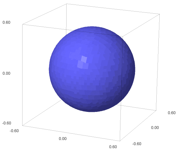
Figure 1: Basic building block

For the example on the right of Fig. 1, the coordinates and string radii are mapped to

$$X=\frac{1}{2}\left(\begin{array}[]{cc}0&1\\ 1&0\end{array}\right)=\frac{1}{2}\sigma_{1},\>Y=\frac{i}{2}\left(\begin{array}[]{cc}0&-1\\ 1&0\end{array}\right)=\frac{1}{2}\sigma_{2},\>Z=\alpha\left(\begin{array}[]{cc}1\\ &-1\end{array}\right)=\alpha\sigma_{3}$$ (3.3)

The factor $\frac{1}{2}$ has been chosen such that $V$ is simply $\left(\begin{array}[]{cc}0&1\\ 0&0\end{array}\right)$.

For this example with arbitrary $\alpha$, it is easy to analytically determine the determinant functional, which results in

$$p=\det\left(\gamma_{a}(X^{a}-x^{a})\right)=r^{4}+z^{4}+2r^{2}(z^{2}+\alpha^{2})+z^{2}(1-2\alpha^{2})+\alpha^{4}-\alpha^{2}$$ (3.4)

with $r^{2}=x^{2}+y^{2}$.

The zero modes surface has a rotational symmetry with respect to $x$ and $y$. For $r=0$ we can determine the coordinates for $z$ via

$$p(r=0)=\left(z^{2}-\alpha^{2}\right)\left(z^{2}-\alpha^{2}+1\right)$$ (3.5)

The $\alpha$-dependent family of zero modes surfaces shows many interesting features, which arise also for the more complicated fuzzy spaces constructed below.

• For $0<\alpha<\frac{1}{2}$ the zero modes surface has the shape of a quenched sphere or disc.

• For $\alpha=\frac{1}{2}$, the zero modes surface is a (real and not only topological) sphere with radius $\frac{1}{2}$ and the polynomial $p$ decomposes into

  $$p=\left(r^{2}+z^{2}-\frac{1}{4}\right)\left(r^{2}+z^{2}+\frac{3}{4}\right)$$ (3.6)

  (In this case, the matrices define the smallest fuzzy sphere.)

• For $\frac{1}{2}<\alpha<1$ the zero modes surface gets more and more narrower in the middle, like a barbell.

• For $\alpha=1$, the zero modes surface has a shape like a 2p-orbital along the $z$-axis or equivalently like a 8-curve rotated about the $z$-axis.

• For $\alpha>1$, the zero modes surface is composed of two disconnected topological spheres, which with increasing $\alpha$ shrink and are more and more remote from each other.

3.2 The general mapping

In general, we have a graph with $N$ nodes, which are labeled with $N$ points $(x_{i},y_{i},z_{i})$. The nodes are numbered, however the following mapping to matrices is covariant under permutations of the numbering of the nodes in the sense that a permutation of nodes results in a permutation of matrix row and line numbers. These permutations are a subgroup of the matrix transformation group under which $\det D_{x}$ is invariant. More general, a permutation of nodes corresponds to a permutation of a basis of the Hilbert space, the matrices act on.

As second ingredient, the graph has directed edges, which interconnect the nodes (only at least one edge interconnects two nodes). The edges are labeled with two complex numbers $(s_{xij},s_{yij})$ , where $i$ and $j$ are the number of the nodes, which are interconnected by the edge.

A graph defined in this way is mapped to three quadratic matrices $X,Y,Z$ of dimension $N$, where we demand that the $2\times 2$ sub-matrices of $X$, $Y$, and $Z$ corresponding to one edge have the form of the basic building block described above. In particular:

• The diagonal entries of the matrices are filled with the coordinates of the points, i.e.

  $$X_{ii}=x_{i},\ Y_{ii}=y_{i},\>Z_{ii}=z_{i}$$ (3.7)

• When the graph has an edge from node $i$ to node $j$, the off-diagonal elements of $X$ and $Y$are filled according to

  $$X_{ij}=s_{xij},\,X_{ij}=\overline{s_{xij}},\quad Y_{ij}=-is_{xij},\,Y_{ji}=i\overline{s_{xij}}$$ (3.8)

• The other entries of the matrices are zero.

The matrices $X$, $Y$ and $Z$ are Hermitian. Note that two graphs with the same nodes and edges but different edge directions are not equal and will not result in equal zero modes surfaces. Changing the direction of an edge corresponds to transposing the corresponding basic building block.

When using the matrix $V=X+iY$, the mapping is

$$V_{ii}=x_{i}+iy_{i}=v_{i},\>Z_{ii}=z_{i}$$ (3.9)

$$V_{ij}=s_{ij}=s_{xij}+s_{yij},\;V_{ji}=s_{ji}=\overline{s_{xij}}-\overline{s_{yij}}$$ (3.10)

Here, changing the direction of an edge from $i$ to $j$ corresponds to exchanging $s_{ij}$ with $s_{ji}$.

For three arbitrary Hermitian matrices it is also possible to provide an inverse mapping that results in a graph with a set of matrices that are equivalent to these matrices up to a unitary transformation. In particular, the three arbitrary matrices and the matrices of the graph have the same zero modes surface:

Since the three arbitrary matrices are Hermitian, one matrix, say $Z$, can be diagonalized with a unitary transformation. The other two matrices $X$ and $Y$ can be transformed with this unitary transformation. From the transformed matrices $X$ and $Y$ and the diagonalized matrix $Z$, the diagonal entries form the points of the graph. For every non-zero diagonal entry of $X$ and $Y$ an edge has to be added to the graph. The labels $s_{x}$ and $s_{y}$ of the edge can be read off from the corresponding matrix entries. Due to the choice of the matrix, which is diagonalized, there are in principle three different graphs associated with three Hermitian matrices.

Interestingly, after diagonalizing $Z$, what remains from the symmetry of unitary transformations are permutations of the eigenvectors (which are basis vectors for the space, on which the matrices act) and phase transformations of the eigenvectors. The permutation of eigenvectors corresponds to a permutation of a numbering of the nodes of the graph, i.e. the mapping is well-defined for graphs with unnumbered nodes.

The phase transformations of the eigenvectors can be encoded with diagonal unitary matrices $U$, i.e. matrices that only have diagonal entries $U_{ii}=e^{i\varphi_{i}}$ with real parameters $\varphi_{i}$. When one transforms the matrices $X$, $Y$ and $Z$ with such a transformation, one sees that the diagonal entries, i.e. the points associated to the nodes, are invariant under these transformations and that the entries for an edge from node $i$ to node $j$ acquire a phase $e^{i(\varphi_{i}-\varphi_{j})}$. Such a unitary transformation therefore can be seen at a first glance as a local $U(1)$ lattice gauge transformation defined on the nodes and acting on the ends of the edges. However, since all unitary transformations correspond to symplectomorphism, also these transformations correspond to coordinate transformations of the zero modes manifold.

In the following, we will illustrate the mapping in more and more complex examples. We will show that, when the entries of the matrices are all substantially of the same magnitude, the graphs define fuzzy spaces with zero modes surfaces that have an analogous topology as the graph. In such a way, we are able to define fuzzy spaces with zero modes surfaces of arbitrary genus.

3.3 Fuzzy cylinder

The algebra relations

$$VV^{\dagger}=V^{\dagger}V=r_{0}^{2}1,\quad[Z,V]=V$$ (3.11)

define an infinite fuzzy cylinder (for example, see [9]) with radius $r_{0}$. A matrix representation of this algebra is

$$V=\sum_{n\in\mathbb{Z}}r_{0}\left|n\right\rangle\left\langle n+1\right|,\quad Z=\sum_{n\in\mathbb{Z}}n\left|n\right\rangle\left\langle n\right|$$ (3.12)

In Fig. 2, the corresponding graph is shown on the left. In the graph we have indicated the $z_{n}$ of the points to the left of the nodes. The $x_{n}$ and $y_{n}$ are all zero. In the below, we will omit zero coordinates and will try to align the nodes of the graphs according to their $z$-coordinate. Furthermore, we have introduced a notation with only one number $s$ labeling an edge. This means that for $i<j$ the corresponding $s_{ij}=s$ and $s_{ji}=0$.

Figure 2: Fuzzy cylinder

The graph in the middle corresponds to a finite fuzzy cylinder of length 5, which in general can be defined by projecting out a finite part of the infinite cylinder with a projector $P=\sum_{n=0}^{N-1}\left|n\right\rangle\left\langle n\right|$. The matrices $Z_{P}=PZP$ and $V_{P}=PVP$ for the finite fuzzy cylinder can be represented by

$$V_{P}=r_{0}\sum_{n=0}^{N-2}\left|n\right\rangle\left\langle n+1\right|,\;Z_{P}=\sum_{n=0}^{N-1}n\left|n\right\rangle\left\langle n\right|$$ (3.13)

To the right of Fig. 2 we have included a picture of the zero modes surface of the middle graph with $s=1$. Interestingly, fuzzy spaces seem not to distinguish between open and closed “manifolds”. Although the matrix elements indicate that the fuzzy cylinder has two open ends, the zero modes surface has closed caps giving it more the shape of a capsule. Again, it is useful to visualize the edges of the graph with a closed string that is emerging at the lowest point $0$, which is a border of the graph, propagating along the inner points and vanishing at the other border point. It should be noted that the zero modes surface has a radius smaller than $1$, although due to $s=1$ one would expect a radius of $1$.

It is also interesting to investigate the zero modes surface of a fuzzy cylinder with one edge reversed. In this case, numerical studies with the computer program of the appendix show that the zero modes surface disconnects into two pieces. For example, the zero modes surface corresponding to a graph with three nodes and two edges pointing away from each other or towards each other with $x_{i}=y_{i}=0$, $z_{i}=i$ and $s=1$ looks like an 2p orbital along the $z$-axis.

3.4 Deformed fuzzy cylinder

We now can modify the fuzzy cylinder by moving the nodes (or the corresponding points) in space and by altering the string radii. In Fig. 3, a graph and its zero modes surface for a cylinder of length $N=6$ is shown, where we have set the radii of the outermost edges to $2$ and where we have moved the two inner node by one unit in $x$-direction. In the graph, we have arranged the nodes according to their $x$ and $z$-coordinates, which are indicated below and to the left of the graph.

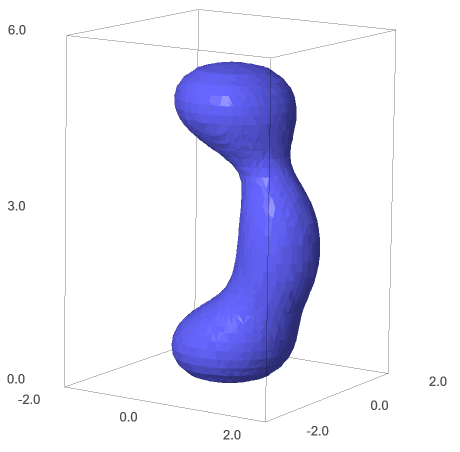
Figure 3: Deformed fuzzy cylinder

The corresponding matrices are

$$V=\left(\begin{array}[]{cccccc}0&2\\ &0&1\\ &&1&1\\ &&&1&1\\ &&&&0&2\\ &&&&&0\end{array}\right)\ Z=\left(\begin{array}[]{cccccc}0\\ &1\\ &&2\\ &&&3\\ &&&&4.5\\ &&&&&5.5\end{array}\right)$$ (3.14)

The edge between $z=3$ and $z=4.5$ has been made longer as the other edges. One sees that elongating the length of an edge results in a smaller radius of the zero modes surface between the two corresponding points. With the computer program, one also can see that there exists an edge length, where the upper part of the zero modes surface disconnects from the lower part.

3.5 Fuzzy sphere

The fuzzy sphere [9, 10] is defined by the representations of $SU(2)$. With $X_{i}=L_{i}/J$ where the $L_{i}$ form the $2j+1$-dimensional representation of the $SU(2)$ and $J=\sqrt{j(j+1)}$ is the root of the Casimir, we can define $V=X_{1}+iX_{2}$ and $Z=X_{3}$. This results in

$$Z = \frac{1}{\sqrt{j(j+1)}}\sum_{m=-j}^{j}m\left|m\right\rangle\left\langle m\right|$$ (3.15)

$$V = \sum_{m=-j}^{j}\sqrt{1-\frac{m(m-1)}{j(j+1)}}\left|m\right\rangle\left\langle m+1\right|$$ (3.16)

The graph of the fuzzy sphere is a simple graph of $N=2j+1$ nodes which are interconnected by $2j$ edges in a line. The node $m$ of the graph is label with $(0,0,m/J)$ and the edge interconnecting node $m$ with node $m+1$ is labeled with $s=\sqrt{1-m(m-1)/J^{2}}$. The fuzzy sphere can be seen as a fuzzy cylinder, which string radii are adjusted, such they fill out a sphere surface. Fig. 4 shows the graph of the fuzzy sphere with $j=2$, where we have visualized the parameters $s$ with circles of radius $s$. We have omitted a picture of the zero modes surface, which is a sphere.

Figure 4: Fuzzy sphere

3.6 Fuzzy torus

We continue with fuzzy spaces of genus 1. The usually described fuzzy torus, which is defined by clock and shift matrices (see, for example [9]), is based on a surface embedded in the four sphere. Although it is possible to define a graph with points in $\mathbb{R}^{4}$ that reproduces this torus, we rather continue with the “deformed fuzzy torus” as described in [8], which is naturally embedded in $\mathbb{R}^{3}$. This fuzzy torus is represented by the matrices

$$Z = \sum_{n=0}^{N-1}\mu\sin\left(\frac{2\pi}{N}(n+\delta)\right)\left|n\right\rangle\left\langle n\right|=\sum_{n=0}^{N-1}z_{n}\left|n\right\rangle\left\langle n\right|$$ (3.17)

$$V = \sum_{n=0}^{N-1}\sqrt{\frac{\mu}{\text{cos}\frac{\pi}{N}}\cos\left(\frac{2\pi}{N}(n+\delta+\frac{1}{2})\right)+\nu}\left|n\right\rangle\left\langle n+1\right|=\sum_{n=0}^{N-1}s_{n}\left|n\right\rangle\left\langle n+1\right|$$ (3.18)

for $\nu>\mu$. Note that in the last equation, $\left|N-1\right\rangle\left\langle N\right|$ is identified with $\left|N-1\right\rangle\left\langle 0\right|$, i.e. $V$ is “cyclic”, which will have interesting consequences in the following. (This is also a property of the shift matrix of the fuzzy torus with embedding in the four sphere.) For $\nu<\mu$ and the index $n$ restricted to real values for the factors $s_{n}$ of $V$ (the value under the square root should be non-negative), the matrices represent a “deformed” fuzzy sphere. However we will concentrate on the case of the deformed torus.

From (3.17, 3.18) immediately follows that the nodes of the graph only have different $z$-coordinates, but all lie on the $z$-axis. Due to the cyclic property of $V$, the associated graph is cyclic and the string radii $s_{n}$ are associated to the edges between node $n$ and node $n+1$ (where $N$ is identified with $0$). Since the deformed fuzzy torus is based on the relation

$$(\frac{VV^{\dagger}+V^{\dagger}V}{2}-\nu)^{2}+Z^{2}=\mu$$ (3.19)

the points $(z_{n},s_{n})$ lie substantially on a deformed circle around the point $(0,\nu)$. In the case of tori, it is a good visualization to draw the nodes of the graphs at the coordinates $(z_{n},s_{n})$ and to assume that the graph is a cross-section of the tori along the half-plane defined by the $z$-axis and the positive half of the $x$-axis. However, it is important to keep in mind that the $x$-coordinate of the visualized node is the string radius of the following edge and not the $x$-coordinate of the point associated to the node.

Fig. 5 shows an example with $N=6$, $\mu=1$ and $\nu=1.5$. The $\mathbb{Z}_{6}$-symmetry of the fuzzy torus is visible.

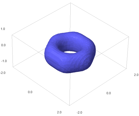
Figure 5: Deformed torus

We also can define a fuzzy version of the standard torus embedded in $\mathbb{R}^{3}$ with the same cyclic graph as the deformed torus but with $s_{n}=\mu\cos\left(\frac{2\pi}{N}(n+\delta)\right)+\nu$. Fig. 6 shows an example with $N=5$, $\mu=1$ and $\nu=1.5$. Our numerical approach shows that for the parameter $\nu$ between $1$ and 1.4, the corresponding zero modes surface does not have a hole in the middle but is bowl shaped.

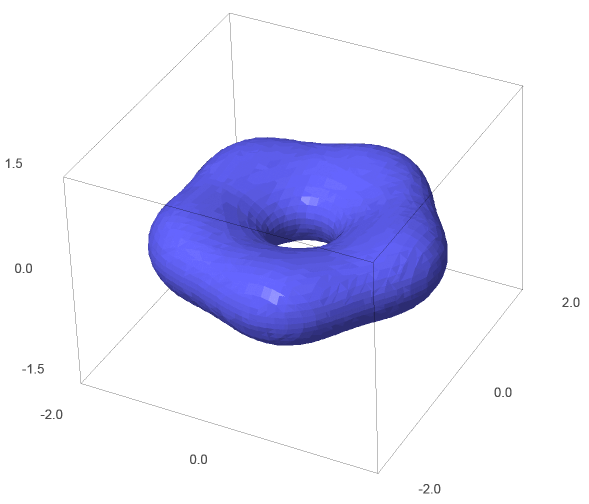
Figure 6: Standard torus

A very simple fuzzy torus can be formed from two fuzzy cylinders of different diameter that are connected at their ends. Fig. 7 shows a torus with $z_{n}=0,1,2,3,2,1$ and $s_{n}=1.5,1.5,1.5,4,4,4$.

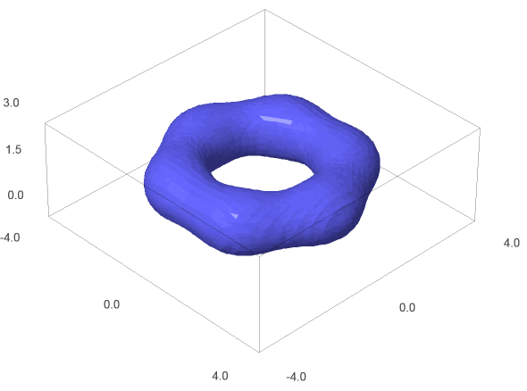
Figure 7: Simple torus

In general, with a spacing for $z_{n}$ about $1$, when the innermost $s_{n}$ approach $1$, the zero modes surface of the tori become more and more a bowl shaped topological sphere. When the $s_{n}$ are getting bigger, the zero modes surface decays into $N$ topological spheres, which centers are aligned equidistant on a circle. For even bigger $s_{n}$, the zero modes surface vanishes (at least as shown by the computer program). The question arises, whether there is still a manifold of minimal dispersion and how this manifold is shaped.

3.7 From cylinder to torus

It is interesting to start with a cylinder and to interconnect the uppermost node with the lowest node by an additional edge. Fig. 8 shows a transformation of a fuzzy torus based on a graph with two nodes at $z=0,1,2$, which are interconnected with two edges labeled by $s=1$. From the left upper plot to the right the string radius $s_{2}$ of an edge between the nodes at $z=0$ and $z=2$ is increased from $0$ to $16$ in steps of $2$. One sees that the fuzzy cylinder transforms in three (in general $N$) small (topological) spheres, which reunite and form a fuzzy torus, when the string radius $s_{2}$ increases. Furthermore, before the spheres are formed, according to the computer program, the zero modes surface vanishes between $s_{2}=1$ and $s_{2}=2$.

The increasing of the string radius $s_{2}$ was explained in [4] as adding strings with maximal angular momentum to the original fuzzy space.

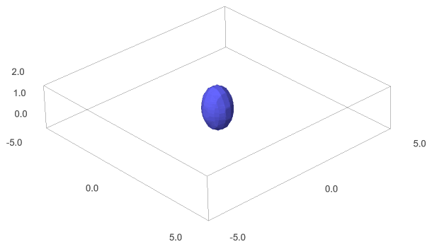
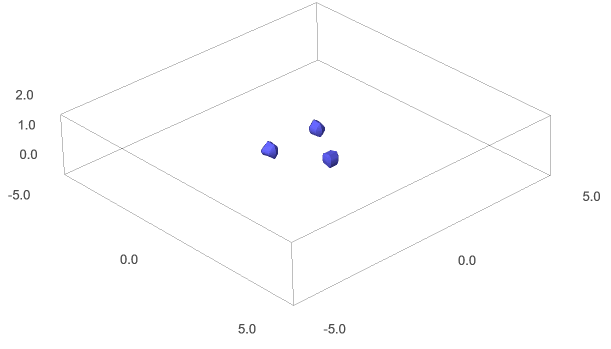
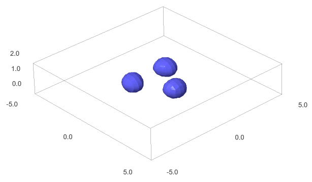
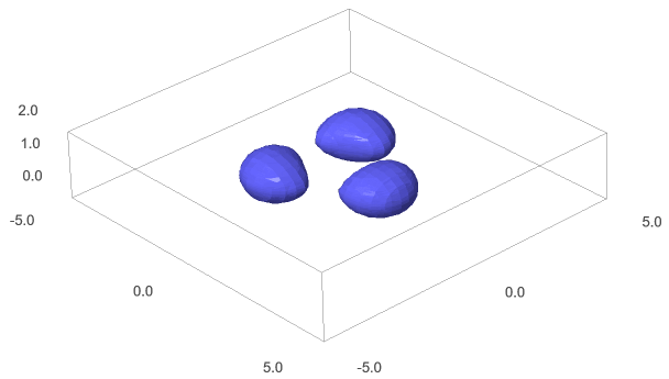
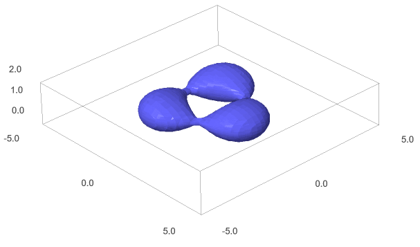
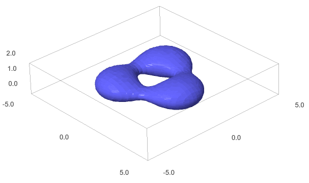
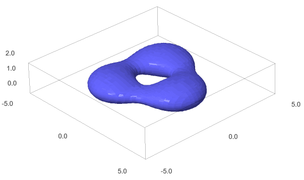
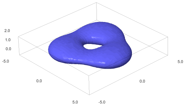
Figure 8: Cylinder transformation

3.8 Fuzzy plane

In three dimensions, with $X=\frac{1}{2}(V+V^{\dagger})$ and $Y=\frac{1}{2i}(V-V^{\dagger})$ the fuzzy plane can be described by

$$V=\sum_{n\in\mathbb{N}_{0}}\sqrt{n+1}\left|n\right\rangle\left\langle n+1\right|,\ Z=0$$ (3.20)

To be consistent, we have renamed the usual lowering and raising operators $A$ and $A^{\dagger}$ to $V$ and $V^{\dagger}$. This infinite dimensional matrices are related to a graph (see Fig. 9) with $\mathbb{N}_{0}$ nodes, in which the points $(x,y,z)$ of all nodes are zero. The $n+1$.th node is connected with the $n$.th node via an edge labeled with $\sqrt{n+1}$. Every node except the first node is connected with two other nodes.

Figure 9: Graph of the fuzzy plane

For calculating the zero modes surface, the zero eigenvalues of

$$D=\left(\begin{array}[]{cc}-z&V^{\dagger}-\bar{v}\\ V-v&z\end{array}\right)$$ (3.21)

have to be calculated, which has been done in [6]. Each eigenstate $\left|v\right\rangle$ of the lowering operator $V$ with $V\left|v\right\rangle=v\left|v\right\rangle$ (which defines the coherent states of the fuzzy plane) can be used to define a zero eigenvector for $D$ for $z=0$

$$\left|\psi\right\rangle=\left(\begin{array}[]{c}\left|v\right\rangle\\ 0\end{array}\right)$$ (3.22)

Since for every $v\in\mathbb{C}$ there is a coherent state $\left|\psi\right\rangle=\exp\left(vV^{\dagger}-\bar{v}V\right)\left|0\right\rangle$, the zero modes surface is the plane $z=0$. As mentioned above, if one projects out a fuzzy disc from the fuzzy plane, the zero modes manifold reduces to the origin.

3.9 Vertices

As we have seen above, fuzzy spaces with genus 0 are based on a graph with two open ends, while fuzzy spaces with genus 1 are based on a simple closed graph forming a loop. We will now extend the graph by a branching, which results in a fuzzy space in the form of a vertex.

Fig. 10 shows the most simple, basic vertex comprising one node, to which three other nodes are connected. To better emphasize the vertex structure, we have reduced $s$ for every edge to $\frac{2}{3}$.

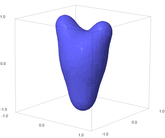
Figure 10: Basic vertex

The corresponding matrices are

$$V=\left(\begin{array}[]{cccc}0&\frac{2}{3}\\ &0&\frac{2}{3}&\frac{2}{3}\\ &&\frac{1}{2}\\ &&&-\frac{1}{2}\end{array}\right)\ Z=\left(\begin{array}[]{cccc}-1\\ &0\\ &&1\\ &&&1\end{array}\right)$$ (3.23)

For $s<\frac{1}{2}$, the three branches of the vertex detach from the central part and the zero modes surface reduces to four topological spheres. Furthermore, the direction of the edges is important. If one of the edges is reversed, then the corresponding part of the zero modes surface detaches from the rest of the zero modes surface.

To the free ends of the basic vertex further nodes can be attached. The result with one further node per branch is shown in Fig. 11.

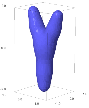
Figure 11: Extended vertex

The corresponding matrices are

$$V=\left(\begin{array}[]{ccccccc}0&\frac{2}{3}\\ &0&\frac{2}{3}\\ &&0&\frac{2}{3}&&\frac{2}{3}\\ &&&\frac{1}{2}&\frac{2}{3}\\ &&&&\frac{3}{4}\\ &&&&&-\frac{1}{2}&\frac{2}{3}\\ &&&&&&-\frac{3}{4}\end{array}\right)\ Z=\left(\begin{array}[]{ccccccc}-2\\ &-1\\ &&0\\ &&&1\\ &&&&2\\ &&&&&1\\ &&&&&&2\end{array}\right)$$ (3.24)

It is possible to add three infinite half cylinders to the basic node, which results in three infinite cylinders meeting in a vertex. The corresponding infinite dimensional matrices are

$$V=\left(\begin{array}[]{ccccccccccc}0&0&s&s\\ s&0&&&0\\ 0&&-x_{0}&&&s\\ 0&&&x_{0}&&&s\\ &s&&&0&&&0\\ &&0&&&-x_{1}&&&s\\ &&&0&&&x_{1}&&&s\\ &&&&s&&&0&&&\ddots\\ &&&&&0&&&-x_{2}\\ &&&&&&0&&&x_{2}\\ &&&&&&&\ddots&&&\ddots\end{array}\right)$$ (3.25)

$$Z=z_{0}\mathrm{\,diag}\left(\begin{array}[]{ccccccccccc}0&-1&1&1&-2&2&2&-3&3&3&\cdots\end{array}\right)$$ (3.26)

where the $x_{1}$ encode the distance from the upper nodes from the $z$-axis and $z_{o}$ is the vertical distance between the nodes.

3.10 Vertical tori

With a vertex it is now possible to construct tori that are aligned vertically, i.e. have a hole that is orthogonal to the $z$-direction. In particular, such a torus can be defined by two vertices that are interconnected with each other with two of their branches. As the other horizontal tori described above, the underlying graphs are also formed of loops. However, for the vertical tori, these loops do have nodes with points that form real loops and are not only restricted to the $z$-axis as the points of the horizontal tori.

A first example of a torus with a graph formed of 6 nodes is shown in Fig. 12.

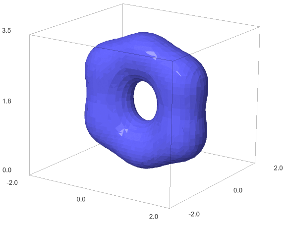
Figure 12: Vertical torus with $\mathbb{Z}_{6}$-symmetry

The matrices are

$$X=\frac{1}{2}\left(\begin{array}[]{cccccc}0&\frac{3}{2}&&&&\frac{3}{2}\\ \frac{3}{2}&-2&1\\ &1&-2&\frac{3}{2}\\ &&\frac{3}{2}&0&\frac{3}{2}\\ &&&\frac{3}{2}&2&1\\ \frac{3}{2}&&&&1&2\end{array}\right)\ Y=-\frac{i}{2}\left(\begin{array}[]{cccccc}0&1&&&&1\\ -1&0&1\\ &-1&0&1\\ &&-1&0&-1\\ &&&1&0&-1\\ -1&&&&1&0\end{array}\right)$$ (3.27)

$$Z=\left(\begin{array}[]{cccccc}0\\ &1\\ &&\frac{5}{2}\\ &&&\frac{7}{2}\\ &&&&\frac{5}{2}\\ &&&&&1\end{array}\right)$$ (3.28)

As a second example, a simple fuzzy vertical torus can be formed of only four nodes. The graph and the zero modes surface of this torus are shown in Fig. 13. The lattice spacing for $z$ and $x$ with $5/4$ and $3/4$ has been chosen to get a zero modes surface that is more symmetric with respect to rotations around the $y$-axis.

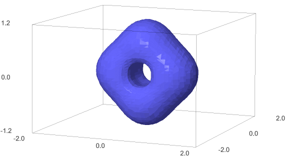
Figure 13: Simple vertical torus with $\mathbb{Z}_{4}$-symmetry

The matrices are

$$V=\left(\begin{array}[]{cccc}0&1&1\\ &\frac{3}{4}&&1\\ &&-\frac{3}{4}&1\\ &&&0\end{array}\right)\ Z=\frac{1}{4}\left(\begin{array}[]{cccc}-5\\ &0\\ &&0\\ &&&5\end{array}\right)$$ (3.29)

We have sorted the nodes in such a way that the matrix $V$ is triangular. This is achieved by sorting the nodes according to their $z$-coordinate. We will see in the following that this is useful for extending the torus to surfaces of higher genus.

3.11 Symmetric fuzzy eight (a genus two surface)

By interconnecting three vertices or two vertical tori we are now able to define fuzzy spaces of higher genus (or fuzzy spaces, which have at least zero modes surfaces of higher genus). Fig. 14 shows the graph and the zero modes surface of a fuzzy space with matrix dimension $N=7,$ which we call “fuzzy eight”. The graphs comprises two closed loops and the zero modes surface has two holes.

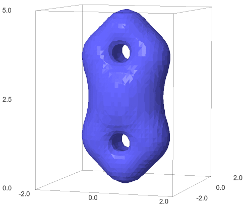
Figure 14: Symmetric fuzzy eight

$$V=\left(\begin{array}[]{ccccccc}0&1&1\\ &\frac{3}{4}&&1\\ &&-\frac{3}{4}&1\\ &&&0&1&1\\ &&&&\frac{3}{4}&&1\\ &&&&&-\frac{3}{4}&1\\ &&&&&&0\end{array}\right)\ Z=\frac{1}{4}\left(\begin{array}[]{ccccccc}0\\ &5\\ &&5\\ &&&10\\ &&&&15\\ &&&&&15\\ &&&&&&20\end{array}\right)$$ (3.30)

In Fig. 15, a section through the zero modes surface at $z=4$, i.e. through the upper hole is shown. The intermediate (blue) line is at $\det D_{x}=0$. The other two (red and green) lines are at $\det D_{x}$ equal to -200,0, and 200. One sees that even for $N=7$, the volume, where the points are nearly zero, is substantially the zero modes surface.

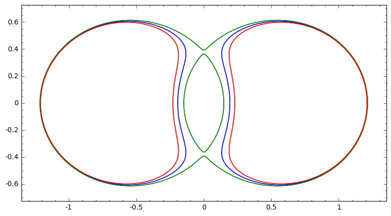
Figure 15: Section through fuzzy eight

Usually, when the fuzzy space is a member of a family of fuzzy spaces, which converge in a specific limit to a classical Poisson manifold, then the genus of the fuzzy space is defined by the genus of the classical manifold. However up to now, there is no mathematical definition for a genus for general non-commutative spaces. In [11] an interesting approach to this problem was considered. It was shown that for the fuzzy torus, i.e. a genus 1 surface, the eigenvalues of matrices have special properties, which there were called “eigenvalue sequences”. This behavior was related to Morse theory.

In the present case of the fuzzy eight, there is per se no commutative limit. However, due to the mapping of the graph to the diagonal $Z$-matrix, the two branches are automatically eigenvalue sequences and one would expect a fuzzy space of higher genus. In general, the branches of the graph can be seen as the eigenvalue sequences of the $Z$-matrix. On the other hand, when one numerically determines the eigenvalues of the $X$-matrix, one sees that there are three equal eigenvalues between one minimal and one maximal eigenvalue, i.e. there are three branches of eigenvalues in the $X$-direction, corresponding to the three hoses interconnecting the left and the right part of the zero modes surface.

3.12 Asymmetric fuzzy eight

A fuzzy space of genus 2 with $N=6$ can be generated with the following matrices, which graph and zero modes surface are shown in Fig. 16.

Figure 16: Asymmetric fuzzy eight

$$V=\left(\begin{array}[]{cccccc}0.8&1&1\\ &0&&1\\ &&1.6&1&1\\ &&&0.8&&1\\ &&&&2.4&1\\ &&&&&1.6\end{array}\right)\ Z=\left(\begin{array}[]{cccccc}0\\ &1.3\\ &&1.3\\ &&&2.6\\ &&&&2.6\\ &&&&&3.9\end{array}\right)$$ (3.31)

3.13 Genus $M$ fuzzy spaces

By extending the symmetric and asymmetric fuzzy eight, it is easy to define matrices, which result in a two-dimensional fuzzy space with genus $m$. An extension of the symmetric fuzzy eight results in the following $3M+1$-dimensional matrices, which define a genus $M$ fuzzy space.

$$V=\left(\begin{array}[]{ccccccccccc}0&1&1\\ &x_{0}&&1\\ &&-x_{0}&1\\ &&&0&1&1\\ &&&&x_{0}&&1\\ &&&&&-x_{0}&1&\ddots\\ &&&&&&0&\ddots\\ &&&&&&&\ddots&1&1\\ &&&&&&&&x_{0}&&1\\ &&&&&&&&&-x_{0}&1\\ &&&&&&&&&&0\end{array}\right)$$ (3.32)

$$Z=z_{0}\mathrm{\,diag}\left(\begin{array}[]{ccccccccccc}0&1&1&2&3&3&4&\cdots&2M-1&2M-1&2M-2\end{array}\right)$$

The parameters $x_{0}$ and $z_{0}$ should be about $1$ to ensure that the holes do not close and that the components of the zero modes surface do not disconnect.

The asymmetric fuzzy eight has an extension with $2M+1$-dimensional matrices, which also define a genus $M$ fuzzy space.

$$V=\left(\begin{array}[]{ccccccccc}x_{0}&1&1\\ &0&&1\\ &&2x_{0}&1&1\\ &&&x_{0}&&1\\ &&&&3x_{0}&1&\ddots\\ &&&&&2x_{0}&\ddots&1\\ &&&&&&\ddots&&1\\ &&&&&&&(M+1)x_{0}&1\\ &&&&&&&&Mx_{0}\end{array}\right)$$ (3.33)

$$Z=z_{0}\mathrm{\,diag}\left(\begin{array}[]{ccccccccc}0&1&1&2&2&3&\cdots&M&M+1\end{array}\right)$$

More general constructions are also possible as shown in Fig. 17.

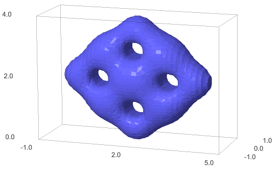
Figure 17: Genus 4 fuzzy surface

4 Conclusions and outlook

We have shown, that directed graphs can be mapped to two-dimensional fuzzy spaces that have similar properties from a topological point of view. Simple graphs can be mapped to fuzzy spaces with zero modes surfaces of genus 0. Graphs forming a loop can be mapped to fuzzy spaces with zero modes surfaces having genus 1. Graphs having branchings and forming more than one loop are mapped to fuzzy spaces with zero modes surfaces of higher genus. Vice versa, it is possible to map every fuzzy space defined by three Hermitian matrices to a graph. We have also shown that this mapping is compatible with the natural symmetry of conjugating unitary matrices with the matrices defining the fuzzy space.

Having now the possibility to define fuzzy spaces of higher genus, thiss can be a basis for defining sequences of graphs that result in fuzzy spaces converging to a classical surface of higher genus in an appropriate limit.

A second point, which can be interesting for further investigation, is a more covariant formulation of the mapping between graphs and matrices. In the moment, the mapping is achieved by firstly diagonalizing $Z$ and secondly constructing the graph from the entries of the transformed matrices $X$ and $Y$. However, the labeling of the nodes or the existence and labeling of an edge of the graph can be derived directly from three general Hermitian matrices.

We also have shown, that the symmetry of conjugating unitary matrices gives rise to $U(1)$ lattice gauge transformations defined on the nodes and acting on the edges. It will be interesting how lattice gauge theories, which simply can be defined on graphs, carry over to gauge theories on the corresponding fuzzy spaces. In this context also the relationship with emerging gravity as described in [13] can be clarified, where the $U(1)$ gauge transformations are interpreted as coordinate transformations in the large $N$ limit.

Finally, aspects of the Standard model and the Higgs mechanism can be formulated in terms of non-commutative geometry (see, for example, [14]). As we now have a mapping from specific non-commutative geometries to graphs, it can be possible to lift the corresponding structures of the Standard model to graphs or generalizations thereof.

Acknowledgments

The author would like to thank Harold Steinacker for illuminating discussions and for reading the manuscript.

Appendix A SageMath program

The following short code listing for SageMath [15] shows how to generate the graphics of the example described in section 3.1. A generalization to bigger matrices or a corresponding program for Mathematica is straightforward.

⬇

Z = Matrix(SR, 2, 2)

Z[0,0]= 0

Z[1,1]= 1

X = Matrix(SR, 2, 2)

X[0,1]= 1/2

X[1,0]= 1/2

Y = Matrix(SR, 2, 2)

Y[0,1]= -I*1/2

Y[1,0]= I*1/2

var(’x,y,z’)

X = X-x

Y = Y-y

Z = Z-z

H=block_matrix(SR,[[Z,X-I*Y],[X+I*Y,-Z]])

p = det(H)

g=implicit_plot3d(p, (x, -1, 1), (y, -1,1), (z, 1,1) )

g.show()

References

- [1] N. Ishibashi, H. Kawai, Y. Kitazawa, and A. Tsuchiya, A Large N reduced model as super- string, Nucl. Phys. B498 , 467 (1997), [hep-th/9612115]
- [2] T. Banks, W. Fischler, S. H. Shenker, and L. Susskind, M theory as a matrix model: A Conjecture, Phys. Rev. D55 , 5112 (1997), [hep-th/9610043]
- [3] A. M. Perelomov, Coherent states for arbitrary Lie group, Comm. Math. Phys. Volume 26, Number 3 (1972), 222-236
- [4] D. Berenstein, E. Dzienkowski, Matrix embeddings on flat and the geometry of membranes, Phys.Rev. D86 (2012) 086001[arXiv:1204.2788 [hep-th]]
- [5] G. Ishiki, Matrix Geometry and Coherent States, Phys.Rev. D92 (2015) no.4, 046009 [arXiv:1503.01230 [hep-th]]
- [6] M. H. de Badyn, J. L. Karczmarek, P. Sabella-Garnier, K. H.-C. Yeh, Emergent geometry of membranes, JHEP 1511 (2015) 089 [arXiv:1506.02035 [hep-th]]
- [7] L. Schneiderbauer, H. Steinacker, Measuring finite Quantum Geometries via Quasi-Coherent States, J.Phys. A49 (2016) no.28, 285301 [arXiv:1601.08007 [hep-th]]
- [8] J. Arnlind, M. Bordemann, L. Hofer, J. Hoppe and H. Shimada, Fuzzy Riemann surfaces, JHEP 0906 (2009) 047 [hep-th/0602290]
- [9] H. Steinacker, Non-commutative geometry and matrix models, PoS QGQGS 2011 (2011) 004 [arXiv:1109.5521 [hep-th]]
- [10] J. Madore, The Fuzzy sphere, 1991, Class.Quant.Grav. 9 (1992) 69-88
- [11] H. Shimada, Membrane topology and matrix regularization, Nucl. Phys. B 685 (2004) 297 [hep-th/0307058]
- [12] F. Lizzi, P. Vitale and A. Zampini, The Fuzzy Disc, JHEP 0308, 057 (2003) [hep-th/0306247]
- [13] 1.H. Steinacker, Emergent Geometry and Gravity from Matrix Models: an Introduction, Mar 2010. 57 pp. Class.Quant.Grav. 27 (2010) 133001 [arXiv:1003.4134 [hep-th]
- [14] G. Cammarata, Robert Coquereaux, Comments about Higgs fields, noncommutative geometry and the standard model, Mar 1995. 20 pp. Lect.Notes Phys. 469 (1996) 27-50 [hep-th/9505192]
- [15] SageMath, the Sage Mathematics Software System (Version 7.0), 2016, [http://www.sagemath.org]