On the $h\to V\ell^{+}\ell^{-}$ decays

Abstract

A set of exclusive decay of the Higgs boson into a vector meson and a dilepton pair ($h\to V\ell^{+}\ell^{-}$, with $V=\Upsilon,J/\psi,\phi$, and $\ell=\mu,\tau$) are studied in the framework of the Standard Model. We have evaluated the decay rates, the dilepton mass spectra and the $V$ longitudinal helicity fraction distributions. In the same framework, we considered the exclusive modes $h\to V\nu\bar{\nu}$ and the implications of the CMS and ATLAS results for the lepton flavor-changing process $h\to\tau^{+}\mu^{-}$ on the $h\to V\tau^{+}\mu^{-}$ decay modes.

1 Introduction

The Higgs-like scalar observed at LHC with $m_{h}=125.7(4)$ GeV Aad:2012tfa ; Chatrchyan:2012xdj ; Agashe:2014kda seems to fulfilled the prediction of the Standard Model (SM) for the Higgs boson. However, it is important to confirm that the couplings of the observed state to the fermions and gauge bosons are what the SM dictates. The couplings of the observed scalar to top and beauty quarks and to $\tau$ leptons are very well studied and are consistent with the SM predictions atlascms ; less known are the couplings to the light quarks and leptons. Many theoretical papers have been devoted to study how to modify these couplings as a consequences of physic beyond the SM Contino:2013kra ; Brivio:2013pma ; Gonzalez-Alonso:2014eva ; Gupta:2014rxa ; Chien:2015xha .

The study of the couplings to the first two generation of fermions is an experimental difficult job. From the theoretical point of view the radiative $h\to f\bar{f}\gamma$ processes have been considered with particular attention. The leptonic modes $h\to\ell^{+}\ell^{-}\gamma$ (with $\ell=e,\mu$) have been considered in Abbasabadi:1996ze ; Chen:2012ju ; Sun:2013rqa ; Dicus:2013ycd ; Passarino:2013nka . While the exclusive channels $h\to V\gamma$, with $V$ a vector meson, have been scrutinized in Bodwin:2013gca ; Kagan:2014ila ; Isidori:2013cla ; Koenig:2015pha , and $h\to VZ$ have been studied in Bhattacharya:2014rra ; Gao:2014xlv as a way to measure the Higgs couplings to the light quarks.

Here we review the results obtained in Colangelo:2016jpi where we have studied the exclusive Higgs decays $h\to V\ell^{+}\ell^{-}$, with $V=\Upsilon,J/\psi,\phi$ and $\ell$ is a light or a heavy charged lepton. The motivations to study these processes are:

1. there is the possibility of considering, in addition to the decay rates, some distributions encoding important physical information, namely the distributions in the dilepton invariant mass squared;

2. due to the fact that several amplitudes contribute to each process, one can look at kinematical configurations where interferences are enhanced in order to get information on the various Higgs couplings;

3. they have a clear experimental signature, although the rates are small;

4. deviations from the Standard Model can also be probed through the search of lepton flavor violating signals.

In the next section we will discuss the diagrams contributing to the $h\to V\ell^{+}\ell^{-}$ processes, the couplings and the hadronic quantities necessary to evaluate them. In section 3 we show the calculation of the amplitudes, while, in section 4, the numerical results on the branching ratios, decay distributions and the fraction of polarized decay distribution are presented and discussed. Finally, we will give our conclusions.

2 The Relevant Diagrams

The amplitudes contributing to the $h\to V\ell^{+}\ell^{-}$ decays contain vertices in which the Higgs couples to quarks, to leptons and to the gauge bosons $Z$ and $\gamma$. In SM such couplings are $g_{hf\bar{f}}=i\,m_{f}/v$ for fermions and $g_{hZZ}=i\,2m_{Z}^{2}/v$ for $Z$ ($v=2m_{W}/g=(\sqrt{2}G_{F})^{-1/2}=246$ GeV is the Higgs field vacuum expectation value). Fig. 1 displays the three kinds of diagrams that must be taken into account.

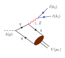
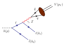
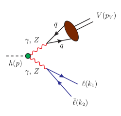
(a)	(b)	(c)

Figure 1: Diagrams contributing to $h\to V\ell^{+}\ell^{-}$ decays. In (a) and (b) the diagrams with $\gamma$ and $Z$ emitted by $\bar{q}$ and $\bar{\ell}$ are considered. In (c) the contributions of the $h\to ZZ$ and the effective $h\to\gamma\gamma$, $h\to\gamma Z$ vertices are considered.

In the diagrams of Fig. 1 (a) we have the Higgs coupled to the quark-antiquark pair. The neutral gauge boson, $\gamma$ or $Z$, is emitted from the quark or the antiquark line before they hadronize in the vector meson $V$. When the dilepton invariant mass squared $q^{2}=(k_{1}+k_{2})^{2}$ is low, the quark hadronization in the vector meson $V$ can be studied by using the formalism of the QCD hard exclusive processes Lepage:1979zb ; Lepage:1980fj ; Efremov:1979qk ; Chernyak:1983ej . Here we should consider the matrix element of the non-local quark antiquark operator while the vector meson state can be expressed as an expansion in increasing twists, which involves various vector meson distribution amplitudes. In the case of $V=\Upsilon,\,J/\psi,\,\phi$, the leading twist light-cone distribution amplitude (LCDA) $\phi_{\perp}^{V}$ is defined from the matrix element of the non-local ${\bar{q}}(y)\sigma_{\mu\nu}q(x)$ quark current:

$$\langle V(p_{V},\,\epsilon_{V})|{\bar{q}}(y)\sigma_{\mu\nu}q(x)|0\rangle=-f_{V}^{\perp}(\epsilon_{V\,\mu}^{*}p_{V\,\nu}-\epsilon_{V\,\nu}^{*}p_{V\,\mu})\int_{0}^{1}du\,e^{i\,u\,p_{V}\cdot x+i\,{\bar{u}}\,p_{V}\cdot y}\phi_{\perp}^{V}(u)$$ (1)

$({\bar{u}}=1-u)$. $u\,p_{V}$ and ${\bar{u}}\,p_{V}$ represent the meson longitudinal momentum fraction carried by the quark and antiquark. $\phi_{\perp}^{V}$ is normalized to $1$; the hadronic parameter $f_{V}^{\perp}$ is discussed below. For more details see Colangelo:2016jpi .
The couplings of the Higgs to leptons are present in the diagrams of Fig. 1 (b), with the $q\bar{q}$ pair emitted by the photon or $Z$. Such diagrams are important in the case of $\tau$. Here the hadronization of the $q\bar{q}$ pair into the vector meson is represented by the matrix element

$$\langle V(p_{V},\,\epsilon_{V})|{\bar{q}}\,\gamma_{\mu}\,q|0\rangle=-if_{V}m_{V}\epsilon^{*}_{V\,\mu}\,\,,$$ (2)

with $p_{V}$ and $\epsilon_{V}$ the $V$ meson momentum and polarization vector, respectively. The experimental measurement of the decay width of $V\to e^{+}e^{-}$ allow to measure the constant $f_{V}$. Less accessible is the hadronic parameter $f_{V}^{\perp}$ in (1) and so results from lattice or QCD sum rule computations must be used. In our analysis we use the range for the ratio $R_{f_{V}}=f_{V}^{\perp}/f_{V}$ quoted in Grossmann:2015lea , obtained exploiting non-relativistic QCD scaling relations Caswell:1985ui ; Bodwin:1994jh :

$$f_{\phi}=0.223\pm 0.0014\,\,\,{\rm MeV}\,\,\,,\hskip 42.67912ptR_{f_{\phi}}=0.76\pm 0.04\,\,,\\$$

$$f_{J/\psi}=0.4033\pm 0.0051\,\,\,{\rm MeV}\,\,\,,\hskip 28.45274ptR_{f_{J/\psi}}=0.91\pm 0.14\,\,,\\$$ (3)

$$f_{\Upsilon}=0.6844\pm 0.0046\,\,\,{\rm MeV}\,\,\,,\hskip 36.98866ptR_{f_{\Upsilon}}=1.09\pm 0.04\,\,.$$

The diagrams of Fig. 1 (c) involve the coupling of the Higgs to a pair of gauge bosons, which in turn are coupled to a lepton pair and to a $q\bar{q}$ pair that hadronizes into $V$. The elementary $hZZ$ coupling can be obtained from the SM Lagrangian. The effective $h\gamma\gamma$ and $hZ\gamma$ vertices can be written as

$$A(H\to G_{1}G_{2})=i\frac{\alpha}{\pi v}C_{G_{1}G_{2}}\left[g_{\mu\nu}(p_{V}\cdot q)-p_{V\mu}q_{\nu}\right]\epsilon_{G_{1}}^{*\mu}\,\,\epsilon_{G_{2}}^{*\nu}\,\,\,,$$ (4)

with $G_{1}$ and $G_{2}$ either $\gamma\gamma$ or $Z\gamma$, and $\epsilon_{G_{1}}$, $\epsilon_{G_{2}}$ polarization vectors. In Eq. (4) $p_{V}$ is the momentum of the meson V and $q$ the momentum of the dilepton. The effective $h\gamma\gamma$ and $hZ\gamma$ couplings are determined by calculations of loop diagrams: $C_{\gamma\gamma}=-3.266+i0.021$ and $C_{\gamma Z}=-2.046+i0.005$ Koenig:2015pha . In the $Z$ propagator we take into account, without considering the uncertainty, the width $\Gamma(Z)=2.4952$ GeV Agashe:2014kda . It is worth remarking that the possibility to access the $hZZ$ coupling is a feature of the class of modes we are analyzing. Moreover, since a sizeable contribution to $h\to V\ell^{+}\ell^{-}$ involves the effective $h\gamma\gamma$ and $hZ\gamma$ couplings from diagrams sensitive to New Physics effects, the exclusive processes also probe deviations from SM.

3 Decay Amplitudes

In this section we give the expressions for the amplitudes corresponding to the diagrams of Fig. 1. At this end, we define

$$C_{\gamma}=4\pi\alpha Q_{\ell}Q_{q}\,\,,\hskip 28.45274ptC_{Z}=\frac{4\pi\alpha}{s_{W}^{2}c_{W}^{2}}\,,$$ (5)

with $s_{W}=\sin\theta_{W}$, $c_{W}=\cos\theta_{W}$, and $\theta_{W}$ the Weinberg angle, and write the propagators in Fig. 1 in terms of the functions

$$D_{1}(a,b,{\hat{q}}^{2})=a+b{\hat{q}}^{2}-ab\,{\hat{m}}_{V}^{2}-{\hat{m}}_{q}^{2}\,,\hskip 25.6073ptD_{2}({\hat{q}}^{2})={\hat{q}}^{2}-{\hat{m}}_{Z}^{2}+i\,{\hat{m}}_{Z}{\hat{\Gamma}}_{Z}\,,\hskip 25.6073ptD_{3}({\hat{k}})=1-2n\cdot{\hat{k}}\,,$$ (6)

where $n=(1,{\vec{0}})$ and we use the notation ${\hat{x}}=\displaystyle{{x}/{m_{h}}}$, $x$ being a mass or a momentum. The lepton current, due to the intermediate gauge boson, has various Dirac structures,

$$V_{\ell}^{\mu}={\bar{\psi}}_{\ell}(k_{1})\gamma^{\mu}\psi_{\bar{\ell}}(k_{2})\,,$$ (7)

for the photon; while for the intermediate $Z$ we have

$$A_{\ell}^{\mu}={\bar{\psi}}_{\ell}(k_{1})\gamma^{\mu}\gamma_{5}\psi_{\bar{\ell}}(k_{2})\,,\hskip 28.45274ptT_{\ell}^{\mu\nu}={\bar{\psi}}_{\ell}(k_{1})\gamma^{\mu}\gamma^{\nu}\psi_{\bar{\ell}}(k_{2})\,,\hskip 28.45274pt{\tilde{T}}_{\ell}^{\mu\nu}={\bar{\psi}}_{\ell}(k_{1})\gamma^{\mu}\gamma^{\nu}\gamma_{5}\psi_{\bar{\ell}}(k_{2})\,.$$ (8)

We write the SM neutral current coupled to the $Z$ boson as

$${\cal L}_{\mu}=\left(-\frac{ie}{s_{W}c_{W}}\right)\left(\Delta_{V}^{f}\,{\bar{f}}\gamma_{\mu}f+\Delta_{A}^{f}\,{\bar{f}}\gamma_{\mu}\gamma_{5}f\right)\,,$$ (9)

where $f$ denotes a fermion, and

$$\Delta_{V}^{f}=\frac{1}{2}\left(T_{3}^{f}-2s_{W}^{2}Q^{f}\right)\,,\hskip 28.45274pt\Delta_{A}^{f}=-\frac{1}{2}T_{3}^{f}\,,$$ (10)

with $T_{3}^{f}$ the third component of the weak isospin and $Q^{f}$ the electric charge of $f$. Diagrams in Fig. 1(a) also involve the integrals over the LCDA of the vector meson $V$:

$$I_{1}=I_{1}({\hat{q}}^{2})=\int_{0}^{1}\,du\,\phi_{\perp}^{V}(u)\left[\frac{1}{D_{1}(1-u,u,{\hat{q}}^{2})}+\frac{1}{D_{1}(u,1-u,{\hat{q}}^{2})}\right]\,,\\$$ (11)

$$I_{2}=I_{2}({\hat{q}}^{2})=\int_{0}^{1}\,du\,\phi_{\perp}^{V}(u)\left[\frac{u}{D_{1}(1-u,u,{\hat{q}}^{2})}+\frac{1-u}{D_{1}(u,1-u,{\hat{q}}^{2})}\right]\,.$$ (12)

We report the various expressions in correspondence with the diagrams in Fig. 1(a), (b) and (c), considering separately the intermediate photon and $Z$ contributions.

• Fig. 1(a), intermediate $\gamma$:

  $$A_{(a)}^{\gamma}=C_{(a)}^{\gamma}m_{h}\epsilon_{V}^{*\alpha}V_{\ell\,\mu}\,\left\{[n_{\alpha}{\hat{p}}_{V}^{\mu}-g_{\alpha}^{\mu}(n\cdot{\hat{p}}_{V})]I_{1}-g^{\mu}_{\alpha}{\hat{m}}_{V}^{2}I_{2}\right\}\,,\hskip 17.07182pt{\rm with}\hskip 17.07182ptC_{(a)}^{\gamma}=\frac{1}{m_{h}^{2}}\frac{\hat{m}_{q}}{v}C_{\gamma}f_{V}^{\perp}\frac{1}{\hat{q}^{2}}\,.$$ (13)

• Fig. 1(a), intermediate $Z$:

  $$A_{(a)}^{Z}=C_{(a)}^{Z}\epsilon_{V}^{*\alpha}\left[\Delta_{V}^{\ell}\,V_{\ell\,\mu}+\Delta_{A}^{\ell}\,A_{\ell\,\mu}\right]\,\left(g^{\mu\alpha}p_{V}^{\sigma}-g^{\alpha\sigma}p_{V}^{\mu}\right)\,\left[n_{\sigma}I_{1}-{\hat{p}}_{V\sigma}I_{2}\right]\,,$$ (14)

  with

  $$C_{(a)}^{Z}=-\frac{1}{m_{h}^{2}}\frac{\hat{m}_{q}}{v}C_{Z}\frac{1}{D_{2}({\hat{q}}^{2})}f_{V}^{\perp}\,\Delta_{V}^{q}\,\,\,.$$ (15)

• Fig. 1(b), intermediate $\gamma$:

  $$A_{(b)}^{\gamma}=C_{(b)}^{\gamma}\epsilon_{V}^{*\alpha}n^{\mu}\left[-\frac{1}{D_{3}({\hat{k}}_{1})}\,T_{\ell\,\mu\alpha}+\frac{1}{D_{3}({\hat{k}}_{2})}\,T_{\ell\,\alpha\mu}\right]\,,\hskip 28.45274pt{\rm with}\hskip 28.45274ptC_{(b)}^{\gamma}=\frac{1}{m_{h}^{2}}\frac{\hat{m}_{\ell}}{v}C_{\gamma}\frac{f_{V}m_{V}}{\hat{m}_{V}^{2}}\,.$$ (16)

• Fig. 1(b), intermediate $Z$:

  $$A_{(b)}^{Z}=C_{(b)}^{Z}\epsilon^{*}_{V\alpha}n_{\mu}\left\{-\frac{1}{D_{3}({\hat{k}}_{1})}\left[\Delta_{V}^{\ell}T_{\ell}^{\mu\alpha}+\Delta_{A}^{\ell}{\tilde{T}}_{\ell}^{\mu\alpha}\right]+\frac{1}{D_{3}({\hat{k}}_{2})}\left[\Delta_{V}^{\ell}T_{\ell}^{\alpha\mu}-\Delta_{A}^{\ell}{\tilde{T}}_{\ell}^{\alpha\mu}\right]\right\}\,,$$ (17)

  with

  $$C_{(b)}^{Z}=\frac{1}{m_{h}^{2}}\frac{\hat{m}_{\ell}}{v}C_{Z}\frac{\Delta_{V}^{q}}{D_{2}({\hat{m}}_{V}^{2})}f_{V}m_{V}\,\,\,.$$ (18)

• Fig. 1(c), two intermediate photons:

  $$A_{(c)}^{\gamma\gamma}=C_{(c)}^{\gamma\gamma}\epsilon_{V}^{*\alpha}[g_{\alpha\mu}(q\cdot p_{V})-m_{h}^{2}n_{\alpha}n_{\mu}]\,V_{\ell}^{\mu}\,,\hskip 28.45274pt{\rm with}\hskip 28.45274ptC_{(c)}^{\gamma\gamma}=\frac{1}{m_{h}^{4}}\frac{\alpha}{\pi v}C_{\gamma\gamma}\,C_{\gamma}\frac{f_{V}m_{V}}{\hat{m}_{V}^{2}}\frac{1}{{\hat{q}}^{2}}\,\,\,.$$ (19)

• Fig. 1(c), two intermediate $Z$:

  $$A_{(c)}^{ZZ}=C_{(c)}^{ZZ}\epsilon^{*}_{V\alpha}\left(\Delta_{V}^{\ell}\,V_{\ell}^{\alpha}+\Delta_{A}^{\ell}\,A_{\ell}^{\alpha}\right)\,,\hskip 17.07182pt{\rm with}\hskip 17.07182ptC_{(c)}^{ZZ}=\frac{1}{m_{h}^{2}}\frac{2{\hat{m}}_{Z}^{2}}{v}C_{Z}\frac{1}{D_{2}({\hat{q}}^{2})}\frac{1}{D_{2}({\hat{m}}^{2}_{V})}\Delta_{V}^{q}f_{V}m_{V}\,.$$ (20)

• Fig. 1(c), intermediate $\gamma\,Z$, with $\gamma$ converting to leptons:

  $$A_{(c)}^{\gamma Z}=C_{(c)}^{\gamma Z}\epsilon_{V}^{*\alpha}[g_{\alpha\mu}(q\cdot p_{V})-m_{h}^{2}n_{\alpha}n_{\mu}]\,V_{\ell}^{\mu}\,,\hskip 14.22636pt{\rm with}\hskip 14.22636ptC_{(c)}^{\gamma Z}=\frac{1}{m_{h}^{4}}\frac{\alpha}{\pi v}C_{\gamma Z}\frac{4\pi\alpha Q_{\ell}}{s_{W}c_{W}}\frac{1}{{\hat{q}}^{2}}\frac{\Delta_{V}^{q}}{D_{2}({\hat{m}}^{2}_{V})}f_{V}m_{V}\,.$$ (21)

• Fig. 1(c), intermediate $Z\,\gamma$, with $Z$ converting to leptons:

  $$A_{(c)}^{Z\gamma}=C_{(c)}^{Z\gamma}\epsilon_{V}^{*\alpha}[g_{\alpha\mu}(q\cdot p_{V})-m_{h}^{2}n_{\alpha}n_{\mu}]\,\left(\Delta_{V}^{\ell}\,V_{\ell}^{\mu}+\Delta_{A}^{\ell}\,A_{\ell}^{\mu}\right)\,,$$ (22)

  with

  $$C_{(c)}^{Z\gamma}=\frac{1}{m_{h}^{4}}\frac{\alpha}{\pi v}C_{\gamma Z}\frac{4\pi\alpha Q_{q}}{s_{W}c_{W}}\frac{1}{{\hat{m}}^{2}_{V}}\frac{1}{D_{2}({\hat{q}}^{2})}f_{V}m_{V}\,\,\,.$$ (23)

The effective couplings $C_{\gamma\gamma}$ and $C_{\gamma Z}$ are defined through Eq. (4).

4 Numerical Analysis

Starting from the expressions obtained in the previous section we are able to compute the widths of the Higgs into the final states. But to calculate the branching fractions is necessary to get rid of the poorly known Higgs full width. One possibility is to use the expression Koenig:2015pha

$${\cal B}(h\to V\ell^{+}\ell^{-})=\frac{\Gamma(h\to V\ell^{+}\ell^{-})}{\Gamma(h\to\gamma\gamma)}{\cal B}(h\to\gamma\gamma)_{exp}\,\,\,$$ (24)

which employs the computed widths $\Gamma(h\to V\ell^{+}\ell^{-})$ and $\displaystyle\Gamma(h\to\gamma\gamma)=\left(\alpha^{2}/(64\pi^{3}v^{2})\right)|C_{\gamma\gamma}|^{2}m_{h}^{3}$ combined with the measurement $\displaystyle{\cal B}(h\to\gamma\gamma)_{exp}=(2.28\pm 0.11)\times 10^{-3}$ Heinemeyer:2013tqa . We obtain

$${\cal B}(h\to\phi\mu^{+}\mu^{-}) = (7.93\pm 0.39)\times 10^{-8}\hskip 17.07182pt{\cal B}(h\to\phi\tau^{+}\tau^{-})=(2.35\pm 0.12)\times 10^{-6}$$

$${\cal B}(h\to J/\psi\mu^{+}\mu^{-}) = (9.10\pm 0.50)\times 10^{-8}\hskip 17.07182pt{\cal B}(h\to J/\psi\tau^{+}\tau^{-})=(1.82\pm 0.10)\times 10^{-6}$$ (25)

$${\cal B}(h\to\Upsilon\mu^{+}\mu^{-}) = (5.60\pm 0.37)\times 10^{-7}\hskip 17.07182pt{\cal B}(h\to\Upsilon\tau^{+}\tau^{-})=(5.66\pm 0.29)\times 10^{-7}\,.$$

The errors in the branching ratios take into account the uncertainties on the LCDA parameters (cfr Colangelo:2016jpi ), on the decay constants $f_{V}$ and on the ratios $R_{f_{V}}$ in Eqs. (3), and the error on ${\cal B}(h\to\gamma\gamma)_{exp}$. The largest contribution to the uncertainties on the branching ratios is due to the uncertainty on ${\cal B}(h\to\gamma\gamma)_{exp}$ amounting to $50-60\%$ of the total error. The uncertainty on $R_{f_{V}}$ constitutes $20-30\%$ of the total error.

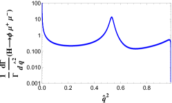
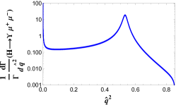
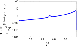
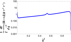
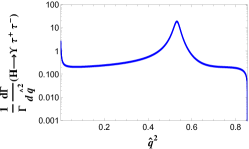
Figure 2: The decay distributions $(1/\Gamma)d{\Gamma}(h\to V\ell^{+}\ell^{-})/d\hat{q}^{2}$, with $\hat{q}^{2}=q^{2}/m_{h}^{2}$ and $q^{2}$ the dilepton mass squared.

The larger rates in Eq. (25) are predicted for modes with $\tau$ pairs, $h\to\phi\tau^{+}\tau^{-}$ and $h\to J/\psi\tau^{+}\tau^{-}$. Due to the smaller coupling, the processes with muons have rates suppressed by a factor 30 and 20, respectively; however, the higher experimental identification efficiency should cancel this suppression.

In the case of $\Upsilon$, the branching ratios with $\tau^{+}\tau^{-}$ and $\mu^{+}\mu^{-}$ are similar. This is an effect of the dominance of the diagram with two intermediate $Z$, Fig. 1 (c), and with coincident contributions. For the $h\to\Upsilon\mu^{+}\mu^{-}$ the next most relevant diagram is the one with the Higgs coupled to quarks, Fig. 1 (a), and it gives contribution very similar to the one coming from the diagram with the Higgs coupled to leptons, Fig. 1 (b), which has the same role for the $h\to\Upsilon\tau^{+}\tau^{-}$ mode.

A comparison with the branching ratios of two body modes is in order. In Koenig:2015pha the authors found ${\cal B}(h\to\phi\gamma)=(2.31\pm 0.11)\times 10^{-6}$ and ${\cal B}(h\to J/\psi\gamma)=(2.95\pm 0.17)\times 10^{-6}$, while ${\cal B}(h\to\Upsilon\gamma)$ is ${\cal O}(10^{-9})$. For the $h\to VZ$ modes, ${\cal B}(h\to\phi Z)\simeq{\cal B}(h\to J/\psi Z)=2.2\times 10^{-6}$ are expected in SM Isidori:2013cla .

In Fig. 2 the decay distributions are plotted in the normalized dilepton mass squared $\hat{q}^{2}=q^{2}/m_{h}^{2}$. The studied modes, with the exception of $h\to\phi\tau^{+}\tau^{-}$ and $h\to J/\psi\tau^{+}\tau^{-}$, are dominated by the virtual photon and $Z$ contributions in Fig. 1 (c). In the $h\to\phi\tau^{+}\tau^{-}$ and $h\to J/\psi\tau^{+}\tau^{-}$ the $\hat{q}^{2}$-distributions show a small $Z$ peak and increase with $\hat{q}^{2}$: an effect of the diagrams with the Higgs coupled to the leptons.
For all the modes the forward-backward lepton asymmetry is very small in the whole range of $\hat{q}^{2}$.

In Fig. 3, the $F_{L}(\hat{q}^{2})=\left(d\Gamma_{L}(h\to V\ell^{+}\ell^{-})/d\hat{q}^{2}\right)/\left(d\Gamma(h\to V\ell^{+}\ell^{-})/d\hat{q}^{2}\right)$ distributions of the fraction of longitudinally polarised vector meson are depicted. $F_{L}\simeq 1$ at the $Z$ mass for the modes with muons in the final state. For the $\phi\tau^{+}\tau^{-}$ and $J/\psi\tau^{+}\tau^{-}$ one can see a narrow peaks in $F_{L}$ for $\hat{q}^{2}=m_{Z}^{2}/m_{h}^{2}$, all the other cases present a smooth $\hat{q}^{2}$ dependence.

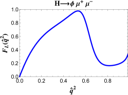
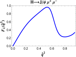
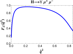
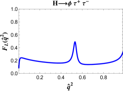
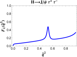
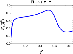
Figure 3: Fraction $F_{L}(\hat{q}^{2})$ of longitudinally polarized meson.

It is quite simple to modify the diagrams in Fig.1 to be able to study the $h\to V\nu\bar{\nu}$ decay widths. Our predictions are the following

$$\centering\hskip 85.35826pt{\cal B}(h\to\phi\nu\bar{\nu})\@add@centering = (1.50\pm 0.075)\times 10^{-7}\,,$$

$${\cal B}(h\to J/\psi\nu\bar{\nu}) = (1.54\pm 0.085)\times 10^{-7}\,,$$ (26)

$${\cal B}(h\to\Upsilon\nu\bar{\nu}) = (1.52\pm 0.08)\times 10^{-6}\,,$$

with a factor $3$ included to account for the neutrino species. The measurements of these decay modes are particularly challenging.

Finally, it is interesting to look at the implications on the processes we have studied of possible lepton flavour violating transition $h\to\tau\mu$. The $h\to\tau\mu$ process has been studied at LHC: for such a mode the CMS Collaboration has published ${\cal B}(h\to\tau\mu)=\left(0.84^{+0.39}_{-0.37}\right)\times 10^{-2}$ together with the upper bound ${\cal B}(h\to\tau\mu)<1.51\times 10^{-2}$ at $95\%$ CL Khachatryan:2015kon , while the ATLAS Collaboration quotes the bound ${\cal B}(h\to\tau\mu)<1.85\times 10^{-2}$ at $95\%$ CL Aad:2015gha . By using the CMS results, the effective coupling, $\kappa_{h\tau\mu}$, can be extracted $\kappa_{h\tau\mu}=(2.6\pm 0.6)\times 10^{-3}$, considering the uncertainties on ${\cal B}(h\to\tau^{+}\mu^{-})$ and ${\cal B}(h\to\gamma\gamma)$. The ATLAS upper bound, instead, implies $\kappa_{h\tau\mu}<3.9\times 10^{-3}$. For these values, the $h\to V\tau^{+}\mu^{-}$ branching fractions and their upper bounds can be computed from the diagrams in Fig. 1 (b):

$$\hskip 56.9055pt{\cal B}(h\to\phi\tau^{+}\mu^{-}) = (3.2\pm 1.5)\times 10^{-7}\,\,\,(<6.9\times 10^{-7})\,,$$

$${\cal B}(h\to J/\psi\tau^{+}\mu^{-}) = (2.4\pm 1.1)\times 10^{-7}\,\,\,(<5.2\times 10^{-7})\,,$$ (27)

$${\cal B}(h\to\Upsilon\tau^{+}\mu^{-}) = (7.2\pm 3.4)\times 10^{-9}\,\,\,(<1.6\times 10^{-8})\,.$$

As one can see by looking at Fig. 4, all the decay distributions have an enhancement at large $q^{2}$.

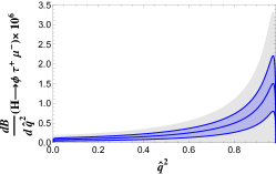
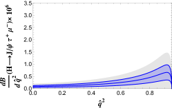
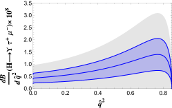
Figure 4: Distributions $d{\cal B}(h\to V\tau^{+}\mu^{-})/d\hat{q}^{2}$ obtained in correspondence to the CMS result for ${\cal B}(h\to\tau^{+}\mu^{-})$ Khachatryan:2015kon . The light shaded area corresponds to the ATLAS bound in Aad:2015gha .

5 Conclusions

For the exclusive decay modes $h\to V\ell^{+}\ell^{-}$ the obtained branching ratios are in the range $10^{-8}\div 10^{-6}$ in SM, of the same order of magnitude of $h\to\phi\gamma$, $h\to\Upsilon\gamma$, $h\to(\phi,J/\psi)\,Z$. The largest rate is predicted for $h\to\phi\tau^{+}\tau^{-}$. The branching ratios of the neutrino modes have been calculated. We have also studied the lepton flavour-changing process $h\to V\tau\mu$ by using the CMS and ATLAS experimental results on the $h\to\tau\mu$ process.

References

- (1) G. Aad et al. (ATLAS), Phys. Lett. B716, 1 (2012), 1207.7214
- (2) S. Chatrchyan et al. (CMS), Phys. Lett. B716, 30 (2012), 1207.7235
- (3) K.A. Olive et al. (Particle Data Group), Chin. Phys. C38, 090001 (2014)
- (4) ATLAS, CMS, ATLAS-CONF-2015-044, CMS-PAS-HIG-15-002 (2015)
- (5) R. Contino, M. Ghezzi, C. Grojean, M. Muhlleitner, M. Spira, JHEP 07, 035 (2013), 1303.3876
- (6) I. Brivio, T. Corbett, O.J.P. Éboli, M.B. Gavela, J. Gonzalez-Fraile, M.C. Gonzalez-Garcia, L. Merlo, S. Rigolin, JHEP 03, 024 (2014), 1311.1823
- (7) M. Gonzalez-Alonso, A. Greljo, G. Isidori, D. Marzocca, Eur. Phys. J. C75, 128 (2015), 1412.6038
- (8) R.S. Gupta, A. Pomarol, F. Riva, Phys. Rev. D91, 035001 (2015), 1405.0181
- (9) Y.T. Chien, V. Cirigliano, W. Dekens, J. de Vries, E. Mereghetti (2015), 1510.00725
- (10) A. Abbasabadi, D. Bowser-Chao, D.A. Dicus, W.W. Repko, Phys. Rev. D55, 5647 (1997), hep-ph/9611209
- (11) L.B. Chen, C.F. Qiao, R.L. Zhu, Phys. Lett. B726, 306 (2013), 1211.6058
- (12) Y. Sun, H.R. Chang, D.N. Gao, JHEP 05, 061 (2013), 1303.2230
- (13) D.A. Dicus, W.W. Repko, Phys. Rev. D87, 077301 (2013), 1302.2159
- (14) G. Passarino, Phys. Lett. B727, 424 (2013), 1308.0422
- (15) G.T. Bodwin, F. Petriello, S. Stoynev, M. Velasco, Phys. Rev. D88, 053003 (2013), 1306.5770
- (16) A.L. Kagan, G. Perez, F. Petriello, Y. Soreq, S. Stoynev, J. Zupan, Phys. Rev. Lett. 114, 101802 (2015), 1406.1722
- (17) G. Isidori, A.V. Manohar, M. Trott, Phys. Lett. B728, 131 (2014), 1305.0663
- (18) M. Koenig, M. Neubert, JHEP 08, 012 (2015), 1505.03870
- (19) B. Bhattacharya, A. Datta, D. London, Phys. Lett. B736, 421 (2014), 1407.0695
- (20) D.N. Gao, Phys. Lett. B737, 366 (2014), 1406.7102
- (21) P. Colangelo, F. De Fazio, P. Santorelli, Phys. Lett. B760, 335 (2016), 1602.01372
- (22) G.P. Lepage, S.J. Brodsky, Phys. Lett. B87, 359 (1979)
- (23) G.P. Lepage, S.J. Brodsky, Phys. Rev. D22, 2157 (1980)
- (24) A.V. Efremov, A.V. Radyushkin, Phys. Lett. B94, 245 (1980)
- (25) V.L. Chernyak, A.R. Zhitnitsky, Phys. Rept. 112, 173 (1984)
- (26) Y. Grossman, M. Koenig, M. Neubert, JHEP 04, 101 (2015), 1501.06569
- (27) W.E. Caswell, G.P. Lepage, Phys. Lett. B167, 437 (1986)
- (28) G.T. Bodwin, E. Braaten, G.P. Lepage, Phys. Rev. D51, 1125 (1995), [Erratum: Phys. Rev.D55,5853(1997)], hep-ph/9407339
- (29) J.R. Andersen et al. (LHC Higgs Cross Section Working Group) (2013), 1307.1347
- (30) V. Khachatryan et al. (CMS), Phys. Lett. B749, 337 (2015), 1502.07400
- (31) G. Aad et al. (ATLAS), JHEP 11, 211 (2015), 1508.03372