Impact of embedding on predictability of failure-recovery dynamics in networks

Abstract

Failure, damage spread and recovery crucially underlie many spatially embedded networked systems ranging from transportation structures to the human body. Here we study the interplay between spontaneous damage, induced failure and recovery in both embedded and non-embedded networks. In our model the network’s components follow three realistic processes that capture these features: (i) spontaneous failure of a component independent of the neighborhood (internal failure), (ii) failure induced by failed neighboring nodes (external failure) and (iii) spontaneous recovery of a component. We identify a metastable domain in the global network phase diagram spanned by the model’s control parameters where dramatic hysteresis effects and random switching between two coexisting states are observed. The loss of predictability due to these effects depend on the characteristic link length of the embedded system. For the Euclidean lattice in particular, hysteresis and switching only occur in an extremely narrow region of the parameter space compared to random networks. We develop a unifying theory which links the dynamics of our model to contact processes. Our unifying framework may help to better understand predictability and controllability in spatially embedded and random networks where spontaneous recovery of components can mitigate spontaneous failure and damage spread in the global network.

I Introduction

Failure, damage spread and recovery crucially underlie many spatially embedded networked systems ranging from transportation structures to the human body Verma et al. (2016); Barabási et al. (2011); Barthélemy (2011). Advances in the study of networks have led to important progress in understanding resilience and controllability in terms of the interaction between topology and various underlying spreading dynamics Cohen et al. (2000); Albert et al. (2000); Centola et al. (2005); Buldyrev et al. (2010); Helbing (2013); Bashan et al. (2013). In the case of a simple contagion or contact process such as an epidemic, it is possible for the disease to spread from a single infected source to other neighboring individuals. On the other hand, many phenomena such as the diffusion of innovations Coleman et al. (1957); Rogers (2010), political mobilization Chwe (1999), viral marketing Leskovec et al. (2007) and coordination games Easley and Kleinberg (2010) are characterized by a complex contagion where nodes need to be connected to multiple sources in order to induce a change of their state Granovetter (1978); Centola and Macy (2007). In addition to this induced transition, individuals may spontaneously change their opinion or banks can spontaneously fail May et al. (2008); Haldane and May (2011).

The consequences of the interplay between spontaneous damage, induced failure and recovery of components in spatially embedded systems are crucial for systemic risk Lorenz et al. (2009), predictability and controllability but have not yet been systematically explored. Many real-world networks such as power grids, computer networks and social networks are embedded in Euclidean space Barthélemy (2011). We here show how the process of embedding and the related characteristic link length impact the predictability of failure-recovery dynamics in networks.

Our model is based on three fundamental processes (i) spontaneous failure independent of the neighborhood (internal failure), (ii) failure induced by failed neighboring nodes if their number exceeds a threshold (external failure) and (iii) spontaneous recovery (see Fig. 1). The interplay between these three processes results in a phase diagram with a metastable regime where hysteresis and switching between two coexisting states are observed Majdandzic et al. (2014). In technological systems, hysteresis effects might be potentially harmful since slight changes of the system’s control parameters can entail drastic and abrupt transitions from a seemingly globally stable state to macroscopic inactivity or large-scale outage Achlioptas et al. (2009); Araújo and Herrmann (2010); Nagler et al. (2011, 2012); Schröder et al. (2013); Cho et al. (2013); Chen et al. (2013a, b); Helbing (2013); Chen et al. (2014); Böttcher et al. (2015); D’Souza and Nagler (2015); Böttcher et al. (2016); Saberi et al. (2016); Schröder et al. (2016). Hysteresis and spontaneous switching between coexisting states in multistable dynamical systems has received great attention for processes ranging from decision making Turalska et al. (2009), multistable perception Ditzinger and Haken (1989); Moreno-Bote et al. (2007); Atwal (2014) over fluid phase transitions Kesselring et al. (2013), protein folding and unfolding Ding et al. (2002) to chemical oscillations Kim et al. (2002), magnetic systems Binder and Landau (1984) and human sleep stages Bashan et al. (2012). We therefore propose here that the extent of the metastable regime in the parameter space of the phase diagram can be regarded as a measure of predictability. The larger the metastable regime the lower is the predictability of the system. Based on this measure we find that the networks’ predictability strongly increases with its regularity. In particular, for the Euclidean lattice, hysteresis only occurs in a very small range of the spontaneous failure rate – compared to random networks with the same average number of neighbors.

Our analytical approach is based on mapping the dynamics to a generalized contact process where a certain minimum number of failed neighboring nodes is necessary to activate the induced failure Tomé and de Oliveira (2015). This strongly suggests that the dynamics does not belong to the Ising universality class as conjectured earlier Majdandzic et al. (2014). In addition, we show that our model system is inherently linked to complex contagion phenomena Granovetter (1978); Centola and Macy (2007) and cusp catastrophes Ludwig et al. (1978); Zeeman (1979); Strogatz (2014). Our unifying framework for random and partially embedded networks helps to better understand predictability and controllability in systems where spontaneous recovery can mitigate spontaneous failure and damage spread.

II Materials and Methods

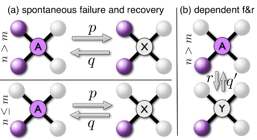
Figure ​​ 1: Model. (a) Spontaneous failure ($A\rightarrow X$) and spontaneous recovery ($X\rightarrow A$) takes place with rates $p$ and $q$, respectively. (b) A node may also fail (become inactive) dependent on its neighborhood, if too few active nodes $n\leq m$ sustain the node’s activity ($A\rightarrow Y$ with rate $r$). In addition, a failed node $Y$ recovers ($Y\rightarrow A$) with rate $q^{\prime}$. Illustration for $m=1$. Active nodes are purple.

We study a modified version of the failure-recovery model proposed in Ref. Majdandzic et al. (2014). Specifically, we consider a fully rate based kinetic Monte Carlo model Gillespie (1976, 1977) instead of, as previously, assuming fixed recovery times $\tau\neq 0$ and $\tau^{\prime}=1$. The system’s components (i.e. nodes) are regarded as either active (not damaged) or inactive (failed). The dynamics is based on three fundamental processes: (i) a node spontaneously fails in a time interval $dt$ with probability $p\text{d}t$ (internal failure), (ii) if fewer than or equal to $m$ nearest neighbors of a certain node are active, this node fails due to external causes with probability $r\text{d}t$ (external failure) and (iii) spontaneous recovery with probability $q\text{d}t$ (internal recovery) or probability $q^{\prime}\text{d}t$ (external recovery). The threshold $m$, similar to threshold rules in complex contagion models Granovetter (1978); Watts (2002); López-Pintado (2008) determines if the neighborhood is critically damaged or healthy (Fig. 1). A low value of $m$ describes the case where a large number of infected neighbors is required in order to sustain the spread of an innovation, opinion or damage. Hence, unlike in an epidemic, where a single infected neighbor can infect a susceptible node, in complex contagion processes spread requires more than one infected neighbor.

Let $a(t)\in[0,1]$ denote the total fraction of failed nodes and $z(t)=1-a(t)$ the fraction of active ones. Thus, $a(t)=u_{\text{int}}(t)+u_{\text{ext}}(t)$ with $u_{\text{int}}(t)$ and $u_{\text{ext}}(t)$ being the fractions of internal and external failure respectively. The total fraction of failed nodes in the stationary state is referred to as $a_{st}$. For the derivation of the mean-field rate equations we assume perfect mixing and first concentrate on the internal failure dynamics. The rate equation of internally failed nodes is given by:

$$\frac{du_{\text{int}}(t)}{dt}=p\left(1-a(t)\right)-qu_{\text{int}}(t),$$ (1)

where the first term accounts for the fact that active nodes internally fail with rate $p$ and the second term corresponds to the recovery of internally failed nodes.

A node is said to be located in a critically damaged neighborhood (CDN) if its number of active neighbors is smaller than or equal to $m$. External failure is only acting on nodes in a CDN. The probability that a node of degree $k$ is located in a CDN is $E_{k}=\sum_{j=0}^{m}\binom{k}{k-j}a^{k-j}(1-a)^{j}$ Majdandzic et al. (2014). Consequently, the time evolution of the external failure is described by:

$$\frac{du_{\text{ext}}(t)}{dt}=r\sum_{k}f_{k}E_{k}\left(1-a(t)\right)-q^{\prime}u_{\text{ext}}(t),$$ (2)

with $f_{k}$ being the degree distribution. The first term describes the failure of active nodes in a CDN with rate $r$ and the second term accounts for recovery of externally failed nodes with rate $q^{\prime}$.

III Results

III.1 Time evolution and phase-switching in embedded systems

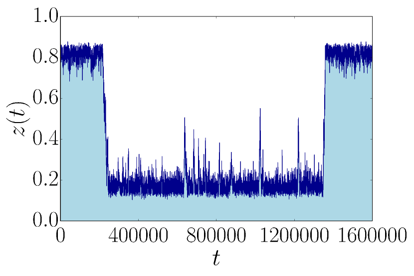
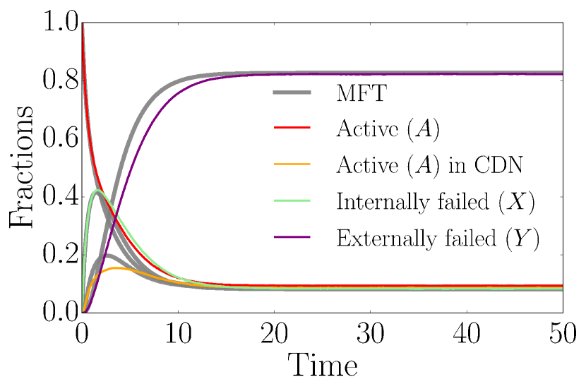
Figure ​​ 2: Model dynamics on a square lattice. (left) Phase switching for $p=0.1065$, $r=0.95$, $q=1.0$, $q^{\prime}=0.1$ and $m=1$ on a square lattice with $N=50\times 50$ nodes ($z$ the fraction of active nodes). (right) Time evolution of different model compartments, i.e. nodes in a certain state (see Fig. 1), with $p=0.9$, $r=0.95$, $q=1.0$, $q^{\prime}=0.1$ and $m=1$ for a square lattice with $N=1024\times 1024$ nodes. All nodes are initially active, $z(0)=1$.

The coupled mean-field rate equations Eqs. (1) and (2) determine the time evolution of the dynamics as shown in Fig. 2. Internal failures first dominate the dynamics but after some time externally induced failures start becoming prevalent in the system. Interestingly, due to the system wide spread of the total failure after a transient phase, indicated by the small fraction of active nodes, the relative abundance of the nodes susceptible to external (active in a CDN) and to internal failure (active) saturate at the same level. However, the process with the higher spreading rate (here external failure with $r/q^{\prime}>p/q$) soon dominates the dynamics. This explains the relatively small contribution of internal failure in this parameter range which could not be observed employing the mean-field theory of Ref. Majdandzic et al. (2014) which assumes that internal and external failure are effectively decoupled processes (case $1\approx\tau^{\prime}\ll\tau$). Therefore, our dynamical theory allows to analytically describe the time evolution of the model’s compartments, i.e. nodes in a certain state.

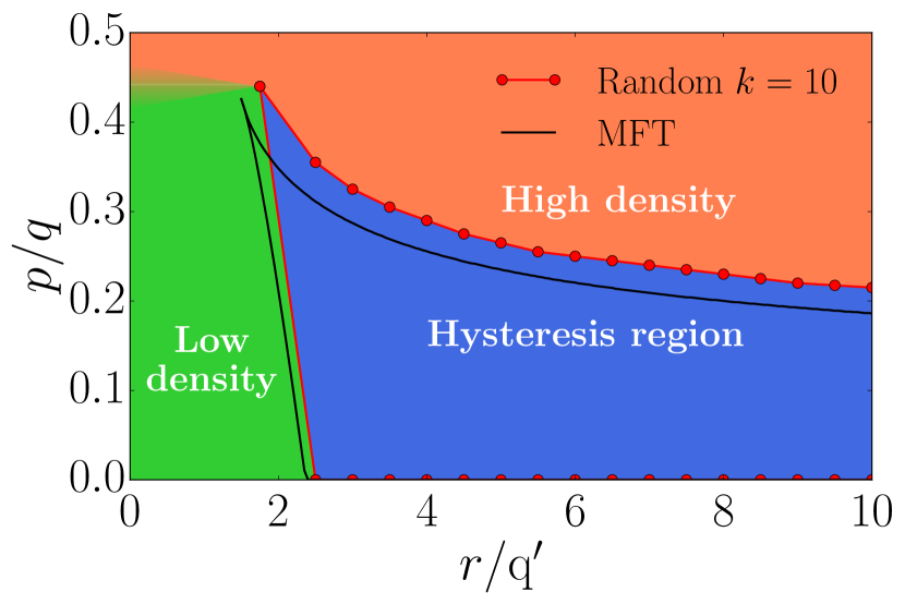
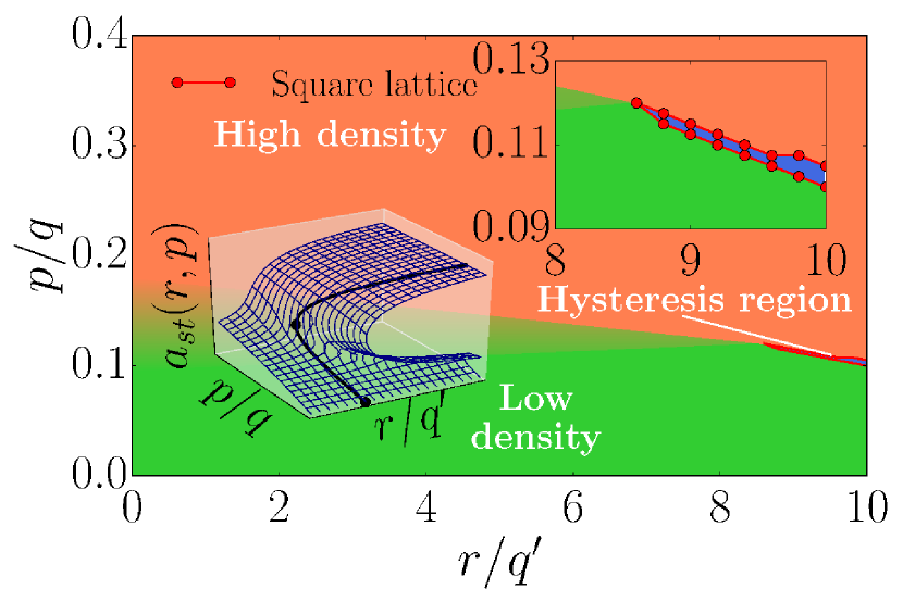
Figure ​​ 3: Phase diagrams of a regular random graph with $k=10$ and a square lattice. (left) The phase space of a regular random graph with $N=100,000$ nodes and $k=10$, $m=4$ (red dots) compared to the mean-field prediction (black lines). (right) The phase diagram of the square lattice (red spinodals) for $m=1$ obtained through simulations on a system with $N=2048\times 2048$ nodes. Inset shows a blow-up of the hysteresis region. Compared to the regular random network (left), this region is very narrow. As an inset in the lower left corner, we show a typical cusp catastrophe surface Zeeman (1979) (mean-field $k=4$, $m=1$) whose bifurcation lines (black) enclose the hysteresis region. For both plots the recovery rates are kept constant ($q=1.0$, $q^{\prime}=0.1$) and $r$, $p$ are varied.

For the Euclidean (square) lattice we observe phase-switching as shown in Fig. 2 (left). The fraction of active nodes $z(t)$ undergoes rapid transitions between a phase of high and low activity. Hysteresis only occurs for large node-to-node spreading rates $r$ and a very narrow range of spontaneous failures rates $p$. Thus, we find the hysteresis region of the lattice to be much narrower than in random graphs as shown in Fig. 3. Inside this metastable domain rapid and unpredictable phase-switching occurs. In addition, crossing this region results in abrupt and dramatic transitions and it might not be possible to go back to the previous state following the same path. As an example, one can consider a nearly healthy population with a varying spontaneous infection rate which can cause the population to undergo a catastrophic transition to a highly infected state by crossing into the hysteresis region. Going back to the healthy state might not be as easy as just retracing the path followed before. In that sense, the extent of the hysteresis region in parameter space can be regarded as a measure for the predictability of the network’s dynamics. The smaller the hysteresis region the less likely it is for the system to end up in this unpredictable situation. However, the unpredictability in the hysteresis region is manifested in two ways: (1) In finite systems, random phase switching between two unstable states is observed where the mean of the random switching times increases exponentially with system size Majdandzic et al. (2014). (2) In the thermodynamic limit no switching is observed but the initial configuration and small random events in the initial temporal evolution of the system determine to which of the two stationary states the system converges. The latter behavior is characteristic for non-self-averaging spin glasses Sherrington and Kirkpatrick (1975); Kirkpatrick and Sherrington (1978); Sornette (2006). As an inset in Fig. 3, we show the relation to cusp catastrophe surfaces accompanying the model’s dynamics. Cusp catastrophes are a prominent example in catastrophe theory describing hysteresis and possible sudden transitions as a consequence of slightly varying control parameters with applications in population dynamics, mechanical and biological systems Ludwig et al. (1978); Zeeman (1979); Strogatz (2014). The bifurcation lines enclose the hysteresis region and merge at the cusp point. The cusp point is a degenerate critical point where not just the first derivative, but also higher derivatives of the potential function vanish. The degeneracy of this critical point can be unfolded by expanding the potential function as a Taylor series in small perturbations of the parameters $r,~{}p,$ and $a$ with a characteristic fourth-order polynomial Zeeman (1979). For a detailed analytical treatment, see Appendices A and B. We define the hysteresis areas enclosed by the bifurcation lines in this parameter range as $A_{H}^{MFT}$ (mean-field) and $A_{H}^{SL}$ (square lattice). The ratio $A_{H}^{MFT}:A_{H}^{SL}\approx 200:1$ shows that the Euclidean lattice is substantially more predictable in the presence of failure and recovery compared to random networks, where non-local connections induce a faster damage spread. For the square lattice, in contrast to random networks, failure cascades are only sustained for a large damage spreading rate r within a narrow region of the ratio $p/q$. To obtain the phase diagram we studied the hysteresis behavior and fluctuations for different fixed values of $r$ by varying $p$. More details about the Euclidean lattice and its critical behavior for different values of $m$ are described in Appendix B. The model’s dynamics is very rich and we show in III.4 that for certain values in the parameter space we encounter closed orbits. We further describe the dynamics and connections to other models, in particular, Schlögl’s first (contact process) and second models and the relation to cusp catastrophes, in Appendix A.

III.2 Spreading dynamics

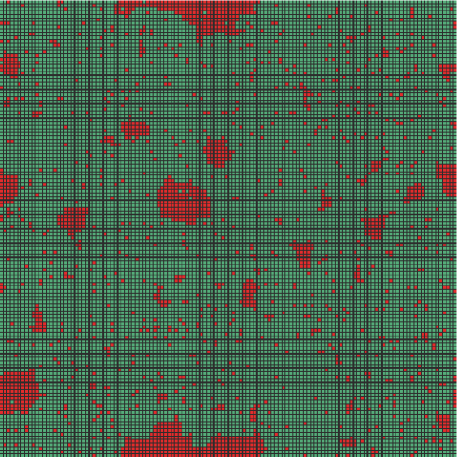
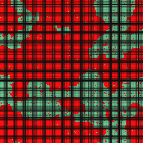
Figure ​​ 4: Nucleation for vanishing spontaneous infection. Simulation of the spontaneous recovery model with $p=0.05$, $q=1.0$, $r=10.0$, $q^{\prime}=0.1$ and $m=1$ on a square lattice with $N=128\times 128$ nodes. (left) Initially, multiple spreading seeds of failed lattice sites (red) form due to spontaneous failure. (right) Contact dynamics (external failure) dominate and active sites (green) are displaced by failed ones (red). For further details we refer to the video version of the dynamics: video 3 (vanishing spontaneous infection).

The dynamics can be driven by the field-like spontaneous failure term or the spread of failure can be triggered by the neighboring failed nodes. We first discuss the dynamics in the hysteresis region of a square lattice with $N=50\times 50$ nodes, cf. Fig. 2. The two mechanisms are illustrated in video 1 (transition down) vid (a) and video 2 (transition up) vid (b). The spontaneous infection term, analogous to an external field, enables the dynamics to form multiple seeds from where the transitions might start. The regions invaded by different seeds expand and move on the lattice. Some of them merge and form larger clusters of active or failed nodes. After some time a stable phase develops.

In the limit of a vanishing external field we expect nucleation determining the growth of a certain phase. Nucleation is exemplified for a small value of $p=0.05$ in Fig. 4. The left side of Fig. 4 (left) displays the initially occurring spreading seeds due to the spontaneous infection dynamics. Eventually, contact dynamics (external failure) leads to a local spread of the failure and larger clusters form as illustrated in Fig. 4 (right). A video of the latter example can be found here: video 3 (vanishing spontaneous infection) vid (c).

III.3 Phase diagrams and transitions for embedded systems

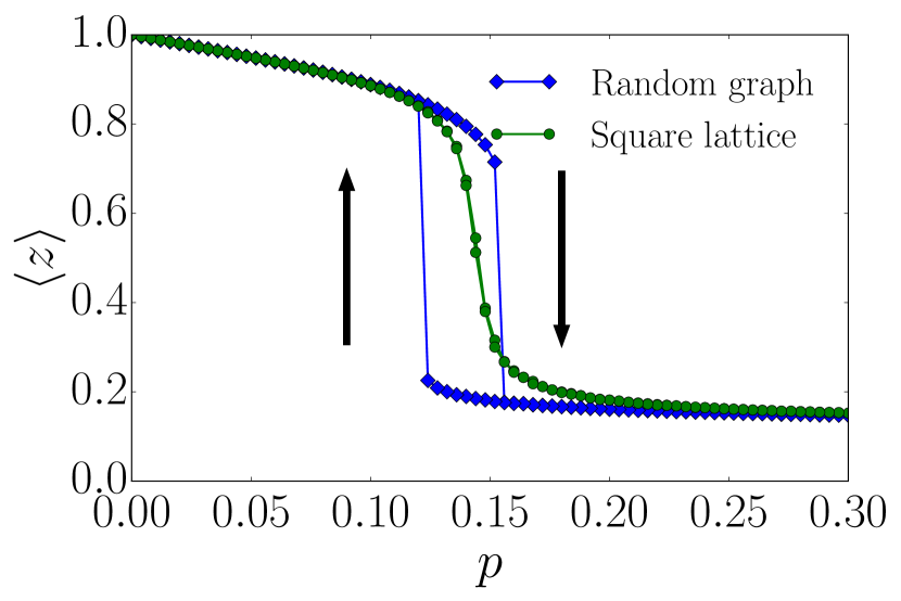
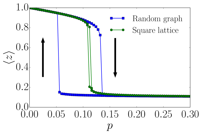
Figure ​​ 5: Illustration of hysteresis effects. Simulation of the failure-recovery model ($\langle z\rangle$ average of the fraction of active nodes) with $q=1.0$, $q^{\prime}=0.1$, $m=1$ for a square lattice and a regular random graph both with $k=4$ and $N=512\times 512$ nodes. (left) The transition is discontinuous for $r=0.7$ for the random graph but continuous for the square lattice. (right) Only for large $r/q^{\prime}$ (shown for $r=1.0$) the transition is discontinuous for both the random graph and the square lattice. The black arrows indicate the direction of the simulation loop.

Critical failure-recovery dynamics necessarily occurs close to the hysteresis region. We study the critical transitions for fixed $r$ and varying $p$ for a regular random graph with degree $k=4$ and for a square lattice. One observes that for $r=0.7$ the square lattice shows a continuous transition whereas the random graph exhibits a discontinuous transition (Fig. 5 (left)). Since in real systems control parameters often can be only determined approximately, this demonstrates that critical failure-recovery dynamics on the lattice can be better controlled compared on a random graph. When both paths cross the hysteresis region, e.g., for $r/q^{\prime}=10$, both dynamics show a discontinuous transition (Fig. 5 (right)). This however requires parameter tuning, that is, large values of the external spreading rate $r/q^{\prime}$.

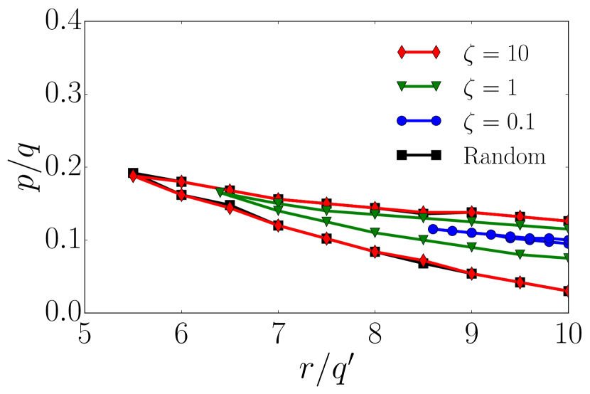
Figure ​​ 6: Phase diagrams of spatially embedded networks with $k=4$ in comparison to a random graph. We set $q=1.0$, $q^{\prime}=0.1$, $m=1$ and perform the simulation for networks with degree $k=4$ and $N=250,000$ nodes. The phase space of a regular random graph with $k=4$ (black squares) is compared to an embedded network with the same degree $k=4$ for different values of the characteristic link length $\zeta$ (blue dots, green inverted triangles, red diamonds). For large $\zeta$ we obtain the phase space of the regular random graph and for small $\zeta$ the square lattice behavior is recovered.

In order to better understand the dramatic differences between random networks and embedded lattices, we analyze here the transition from a square lattice to a regular random graph. To this end, we follow the transition model of Danziger et al. Danziger et al. (2015) and study the phase space of an embedded system with degree $k=4$ where randomly chosen nearest-neighbor links are replaced by longer-range links. The lengths $l$ of the links are distributed according to an exponentially decaying distribution $P(l)\sim\exp\left(-l/\zeta\right)$, with a link length $l$ and characteristic link length $\zeta$. In the thermodynamic limit, a square lattice in the limit of $\zeta\rightarrow 0$ is recovered, whereas in the limit of $\zeta\rightarrow\infty$ we obtain a regular random graph (as all link lengths are equally likely). The phase diagrams of an embedded system with $k=4$ and exponential link length distribution, in the presence of processes (i-iii), are shown in Fig. 6. We clearly observe the transition from a situation similar to the square lattice for $\zeta=0.1$ to a regular random graph for $\zeta=10$. This again illustrates the strong dependence of the extent of the metastable region on the topology. In other words, a variation in the characteristic link length $\zeta$ causes a very narrow metastable domain ($\zeta=0.1$) to expand into a substantially larger region ($\zeta=10$). Therefore, the results presented in this section have implications for the understanding of the predictability of networks.

III.4 Oscillatory behavior

We will briefly describe the possibility of encountering limit cycles in our dynamics. We investigate this behavior by studying the Lyaponuv function Strogatz (2014). In our case, the Lyapunov function $V(a,u_{int})$ is derived from the following equations ($\alpha,\beta>0$):

$$\frac{da(t)}{dt}=-\alpha\frac{\partial V(a,u_{int})}{\partial a},$$ (3)

$$\frac{du_{int}(t)}{dt}=-\beta\frac{\partial V(a,u_{int})}{\partial u_{int}},$$ (4)

which are equivalent to

$$\frac{da(t)}{dt}=r\sum_{k}f_{k}E_{k}\left(1-a(t)\right)+p\left(1-a(t)\right)-qu_{int}(t)-q^{\prime}\left(a-u_{int}(t)\right),$$ (5)

$$\frac{du_{int}(t)}{dt}=p\left(1-a(t)\right)-qu_{int}(t).$$ (6)

Without loss of generality, we set $\beta=1$ and compute $V\left(a,u_{int}\right)$ to:

$$\begin{split}&V\left(a,u_{int}\right)=q\frac{u_{int}^{2}}{2}-pu_{int}\left(1-a\right)-\frac{p}{q-q^{\prime}}\left[p\left(a-\frac{a^{2}}{2}\right)-q^{\prime}\frac{a^{2}}{2}+\right.\\ &r\left.\sum_{k}f_{k}\sum_{j=0}^{m}\sum_{l=0}^{j+1}\binom{k}{k-j}\binom{j+1}{l}(-1)^{l}\frac{a^{k-j+l+1}}{k-j+l+1}\right],\end{split}$$ (7)

where we used the binomial theorem and set $\alpha=\left(q-q^{\prime}\right)/p$. We find that

$$\begin{split}&\frac{dV\left(a,u_{int}\right)}{dt}=\frac{da(t)}{dt}\frac{\partial V\left(a,u_{int}\right)}{\partial a}+\frac{du_{int}(t)}{dt}\frac{\partial V\left(a,u_{int}\right)}{\partial u_{int}}\\ &=-\alpha\left(\frac{\partial V\left(a,u_{int}\right)}{\partial a}\right)^{2}-\beta\left(\frac{\partial V\left(a,u_{int}\right)}{\partial u_{int}}\right)^{2}<0,\end{split}$$ (8)

if $q>q^{\prime}$ since $\beta=1$.

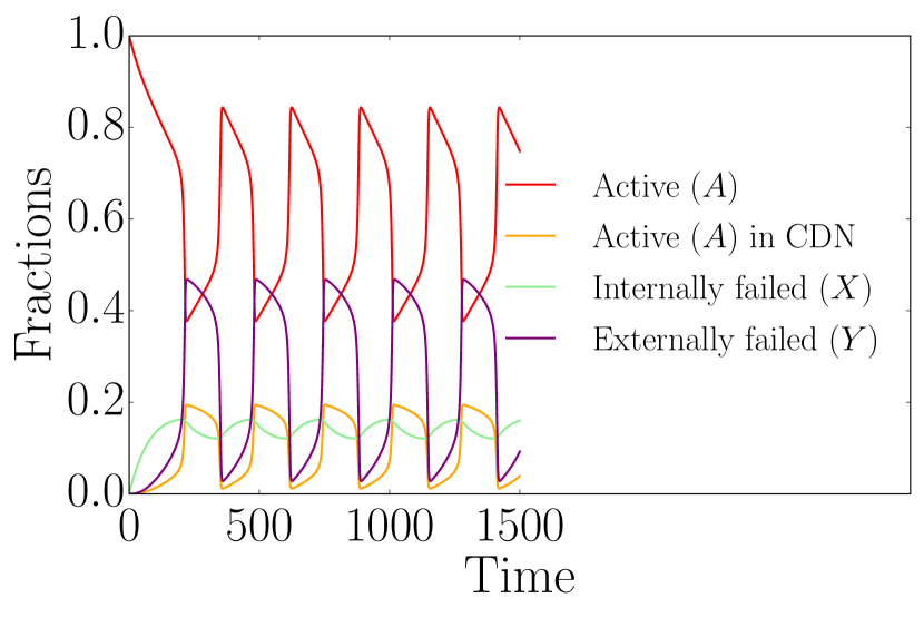
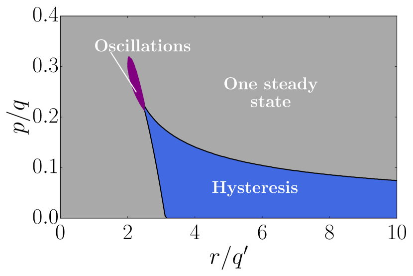
Figure ​​ 7: Oscillatory behavior (limit cycles) for $q^{\prime}>q$. (left) We show the mean-field time evolution of different compartments, cf. Fig. 1, for $p/q=19/81$, $q=0.01$, $r/q^{\prime}=3125/1296$, $q^{\prime}=1.0$, $k=4$ and $m=1$. The values of $p$ and $r$ correspond to the ones of the bifurcation point as described in Appendix B. We clearly see the oscillatory behavior as a consequence of $q^{\prime}>q$. (right) The phase space for $k=4$, $q=0.01$, $q^{\prime}=1.0$ and $m=1$ now also displays an oscillatory regime (purple).

For $q>q^{\prime}$ we therefore expect no oscillatory behavior, i.e. no closed orbits. However, for $q^{\prime}>q$, we show in Fig. 7 the existence of closed orbits. The purple region in Fig. 7 (right) illustrates the regime where we measured a periodic orbit analyzing the Fourier transformed time evolution of the fraction of active nodes. We also show the oscillatory dynamics of a non-embedded regular network in video 4 (oscillations) vid (d). As discussed in Appendix A, for $q=q^{\prime}$, the differential equations Eqs. (1) and (2) can be decoupled and one obtains a single first-order differential equation which has no periodic solutions Strogatz (2014).

This demonstrates that the phase diagram is substantially more complex than previously believed. Specifically, limit cycles occur for $q^{\prime}/q<1$ in a narrow region in the phase diagram. This deterministic behavior is markedly different from the stochastic switching dynamics in the hysteresis region but likewise challenges control.

IV Discussion

We have derived a unifying framework for the interplay between failure, damage spread and recovery in spatially embedded and random networks. The theoretical description links diverse phenomena such as complex contagion and phase-switching due to metastability and the occurrence of cusp catastrophes. The number of failed neighbors necessary to allow external failure to act on a node is a crucial parameter of the system. Our analysis revealed that the phase space is substantially more complex than previously known owing to the coexistence of limit cycles and random phase switching within hysteresis.

We analytically demonstrated that the mean-field description of the stochastic model systems is equivalent to cusp catastrophes with two bifurcation lines enclosing a metastable domain where two stable stationary states coexist. Inside this metastable region, large fractions of nodes suddenly fail and recover. We propose the hysteresis (metastable) area as a predictability measure for the state of the system of a given topology and dynamics. Our results show that the transition from a random regular network to an embedded network with a short characteristic link length is characterized by a dramatic shrinking of the metastable domain. This suggests that embedded systems with short characteristic link lengths whose dynamics is captured by processes (i-iii) are substantially more robust against abrupt spontaneous and cascading failures compared to non-embedded systems.

Moreover, we have also shown that our theoretical framework is able to describe essential features of the model’s time evolution and that it captures spontaneous failure as an external field in analogy to magnetic systems. However, based on the connection to contact process dynamics we find that the model does not belong to the Ising universality class as conjectured earlier Majdandzic et al. (2014). The arguments in Appendices A and B show the similarities to the (non-equilibrium) contact process belonging to the directed percolation universality class Henkel et al. (2008). In fact, as mentioned by Grassberger Grassberger (1982), relating this dynamics to the Ising universality class would mean an extension of the universality hypothesis from models with detailed balance to models without it. Unpredictability observed in the hysteresis region results from two effects. For finite systems, unpredictable random phase switching between two unstable states is observed. In the thermodynamic limit, however, small fluctuations in the initial phase of the systems dynamics determine the stationary (stable) state of the system.

Our framework helps to better understand predictability and controllability in spatially embedded and random systems where spontaneous recovery, spontaneous failure and cascading failure lead to a remarkably complex dynamic interplay.

Author contribution statement

L.B. carried out computational simulations, analytical calculations and wrote the first draft of the manuscript. All authors contributed equally to the ideas, the interpretation and the presentation.

Additional information

Competing financial interests The author(s) declare no competing financial interests.

Appendix A Connection to other models

To draw a connection to other models we first simplify the two coupled rate equations Eqs. (1) and (2). We therefore set $q=q^{\prime}=1$ (excluding limit cycles, cf. Sec. III.4) and add Eqs. (1) and (2) to obtain:

$$\frac{da(t)}{dt}=r\sum_{k}f_{k}E_{k}\left(1-a(t)\right)+p\left(1-a(t)\right)-a(t).$$ (9)

In the limit of a regular degree distribution with $k=1$ and $m=0$, and under the assumption of dynamically rewiring links between nodes, we find exact correspondence to the contact process dynamics with spontaneous infection Marro and Dickman (2005):

$$\frac{da(t)}{dt}=ra(t)\left(1-a(t)\right)+p\left(1-a(t)\right)-a(t).$$ (10)

The latter equation describes nothing but contact process dynamics with a smeared out second order phase transition transition due to the additional spontaneous infection term. We illustrate the stationary state $a_{st}(r)$ (order parameter) as a function of the external failure rate $r$ in Fig. 8 (left). In the limit of vanishing spontaneous failure $p\rightarrow 0$ one encounters a second order phase transition. At the critical point $r_{c}=1$ the order parameter grows as $a_{st}(r)\propto(r-r_{c})^{\beta}$ with $\beta=1$. A non-zero spontaneous failure term leads to a smeared out transition. This situation is similar to the one in the Ising model with an applied magnetic field which also removes the second order phase transition. However, unlike in the Ising model the field equivalent satisfies the condition $p>0$ and we are restricted to one of the two roots defining the stationary state of Eq. (10):

$$a_{st}(r,p)=\frac{1}{2r}\left[r-p-1+\sqrt{(r-p-1)^{2}+4rp}\right].$$ (11)

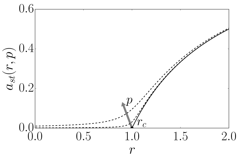
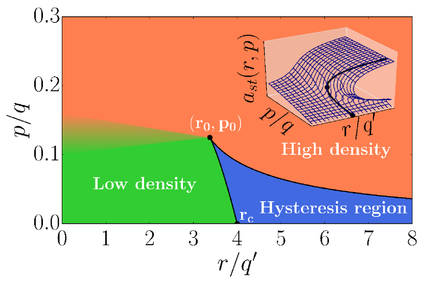
Figure ​​ 8: Analogy to the contact process and Schlögl’s second model. (left) The order parameter $a_{st}(r)$ as a function of the external failure rate $r$ for $k=1$ and $m=0$ (mean-field). Analogous to the contact process the black solid line corresponds to the situation where the vanishing spontaneous infection term $p\rightarrow 0$ leads to a second-order phase transition at $r=r_{c}$. The dashed lines show a smeared out transition due to the non-zero spontaneous infection rates $p=0.001,0.01$ Marro and Dickman (2005). (right) The phase space for $k=2$ and $m=0$ (mean-field). One clearly sees the hysteresis region where two states coexist (low density and high density failure phases). The spinodals (black solid lines) merge at the bifurcation point $(r_{0},p_{0})=(27/8,1/8)$. The critical point, $r_{c}=4$ indicates the transition point without additional field-like term ($p=0$). This situation is similar to Schlögl’s second model Grassberger (1982), the phase space of cusp catastrophes or imperfect bifurcations Strogatz (2014).

Close to the critical point $r_{c}=1$, i.e. $r\rightarrow r_{c}$, we find $a_{st}(r_{c},p)\propto p^{1/\delta_{h}}$ with the field exponent $\delta_{h}=2$ in the mean-field situation.

In order to see the influence of the coupling parameter $m$ on the dynamics, we now turn towards the case $k=2$ and are free to set $m=0,1,2$. For $m=2$ all neighborhoods are critically damaged by definition and the stationary state is given by $a_{st}(r,p)=(r+p)/(1+r+p)$. In particular, this solution is obtained for all regular graphs with degree $k$ and $m=k$ since $E_{k}=\sum_{j=0}^{k}\binom{k}{k-j}a^{k-j}(1-a)^{j}=1$.

The situation is different for $m=1$ where at least one neighbor of a given node needs to fail in order to allow external failure acting on the node. This is again in accordance with the contact process where also at least one failed neighbor is necessary to turn on the spreading dynamics. We also find the corresponding exponents $\beta=1$ and $\delta_{h}=2$ in the vicinity of $r_{c}=1/2$. In general, we expect this behavior for any regular graph with degree $k$ and $m=k-1$ since $\lim_{a\rightarrow 0}E_{k}=\sum_{j=0}^{k-1}\binom{k}{k-j}a^{k-j}(1-a)^{j}=ka+\mathcal{O}(a^{2})$ (at the critical point). That is the reason why we again find the contact process exponents in the latter example and a critical value of $r_{c}=1/2$ which is just the critical point of Eq. (10) divided by $k$.

Another interesting behavior is found for $m=0$. Without spontaneous failure term, the rate equation describes a pair-creation contact process Tomé and de Oliveira (2015) and taking this term into account yields a variant of Schlögl’s second model Grassberger (1982); Vellela and Qian (2009). Setting $p=0$, the stationary state for $r>r_{c}=4$ is given by $a_{st}(r)=1/2(1+\sqrt{1-4/r})$ and $a_{st}(r)=0$ for $r<r_{c}$. The phase diagram for $m=0$ and $p\geq 0$ is illustrated in Fig. 8 (right). Two spinodals define the hysteresis region where two states coexist. As for cusp catastrophes Strogatz (2014), this region is the projection of the hysteresis set from three dimensions into plane space, cf. inset in Fig. 8 (right). In this example, the spinodals are defined by $\Delta=0$ where the discriminant $\Delta=-r(4+4p^{3}-r+4p^{2}(3+2r)+4p(3-5r+r^{2}))$. For $\Delta<0$ two stable coexisting steady states exist while for $\Delta>0$ there is only one. The spinodals merge at the bifurcation point (cusp point) characterized by $(r_{0},p_{0})=(27/8,1/8)$ where $\lim_{(r,p)\rightarrow(r_{0},p_{0})}\partial r/\partial a=0$. At the bifurcation point the quantity $\Delta a_{st}(r,p_{0})=a_{st}(r,p_{0})-a_{st}(r_{0},p_{0})$ increases with $r$ as $\Delta a_{st}(r,p_{0})\propto(r-r_{0})^{\tilde{\beta}}$ and with $p$ as $\Delta a_{st}(r_{0},p)=a_{st}(r_{0},p)-a_{st}(r_{0},p_{0})\propto(p-p_{0})^{1/\tilde{\delta_{h}}}$ where $a_{st}(r_{0},p_{0})=1/3$, $\tilde{\beta}=1/3$ and $\tilde{\delta_{h}}=3$. For this example, it is straightforward to show that the quadratic term in the Taylor expansion of $f(a_{st},r,p)=ra_{st}^{2}(1-a_{st})+p(1-a_{st})-a_{st}$ around $a_{st}(r_{0},p_{0})=1/3$ vanishes yielding the characteristic polynomial of the cusp catastrophe Zeeman (1979). In general, the spontaneous recovery model resembles the dynamics of a modified contact process where a certain minimum number of nodes is necessary to turn on the spreading dynamics Tomé and de Oliveira (2015). As already mentioned in previous studies and as discussed in the latter examples, slight modifications of the standard contact process dynamics might have dramatic effects on the system’s dynamics leading to uncontrollable abrupt transitions Böttcher et al. (2015, 2016).

Appendix B Critical behavior on the square lattice

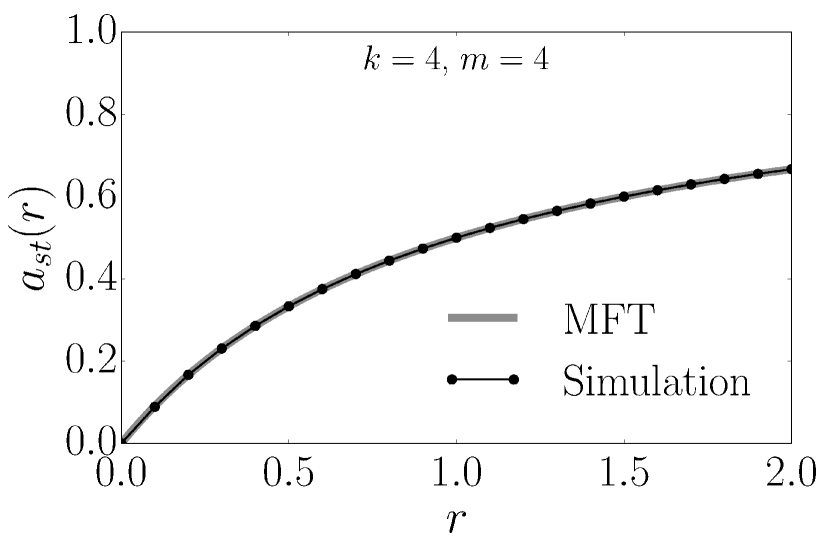
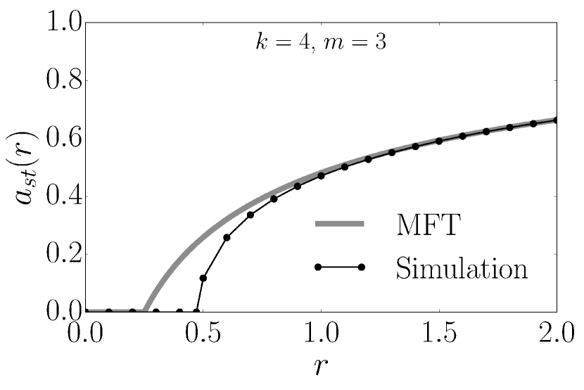
Figure ​​ 9: Growth of the order parameter on a square lattice for different $m$. Simulation of the spontaneous recovery model without internal failure dynamics ($p=0$) and $q^{\prime}=1.0$ for different $m$. (left) The order parameter $a_{st}(r)$ as function of $r$ for $m=4$ and (right) for $m=3$. The simulations have been performed on a square lattice with $N=1024\times 1024$ nodes.

We will now study the critical behavior of the dynamics in a system with degree $k=4$ since there are four nearest-neighbors for every node on a square lattice. Consequently, we have five possibilities of choosing $m=0,1,2,3,4$.

We start with the case $m=4$ for which a CDN even exists when there is no failed neighboring lattice site, i.e. external failure acts all the time independent of the nearest-neighbors’ state, cf. Appendix A. Setting $q^{\prime}=1.0$, the MFT yields for the stationary state of failed nodes $a_{st}(r)=r/(1+r)$ (without field-like spontaneous failure). As long as $r>0$ we find a non-zero fraction of failed nodes in the network. We see in Fig. 9 (left) that the results obtained through simulations on a square lattice are well described by the MFT. An additional field-like contribution of the spontaneous failure $p$ and $q=1.0$ yields $a_{st}(r)=(r+p)/(1+r+p)$, cf. Appendix A.

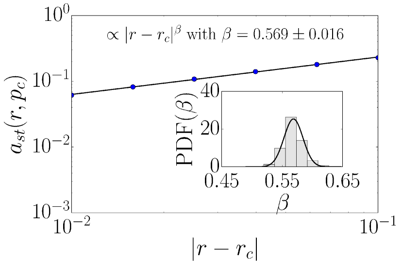
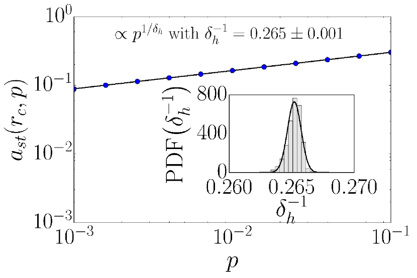
Figure ​​ 10: Critical exponents of the square lattice with $m=3$. Simulation of the spontaneous recovery model with $p=0$, $q^{\prime}=1.0$ and $m=3$. (left) The order parameter $a_{st}$ in the vicinity of the critical point $r_{c}=0.47(1)$ for different $r$. The exponent found indicates contact process dynamics where $\beta=0.586(14)$ Moreira and Dickman (1996). (right) The order parameter $a_{st}$ at the critical point $r_{c}=0.47(1)$ for small values of $p$. The critical exponent measured also indicates contact process dynamics with $\delta_{h}^{-1}=0.285(35)$ Adler and Duarte (1987). The simulations have been performed on a square lattice with $N=1024\times 1024$ nodes ($1500$ samples). The insets show the PDF’s of the exponent’s bootstrap analysis.

For $m=3$ we expect to find dynamics analogous to the contact process, since only one failed neighbor is needed to let the neighboring nodes fail. This has been described in Appendix A and a non-zero stationary state $a_{st}(r)$ is found if $r>r_{c}$ ($r_{c}=1/4$ MFT). From MFT we also find $a_{st}(r)\propto(r-r_{c})^{\beta}$ with $\beta=1$. At $r_{c}$ the order parameter grows continuously. Applying the field term in this example one finds $a_{st}(r_{c},p)\propto p^{1/\delta_{h}}$ with $\delta_{h}=2$. We show the order parameter $a_{st}(r)$ as a function of $r$ for the square lattice in comparison with MFT in Fig. 9 (right). We also analyzed the critical behavior in the vicinity of the critical point $r_{c}=0.47(1)$ of the square lattice (see Fig. 9 (right)). The growth of the order parameter with $\beta=0.569(16)$ (Fig. 10 (left)) and $\delta_{h}^{-1}=0.265(1)$ (Fig. 10 (right)) agrees with the corresponding contact process values $\beta=0.586(14)$ Moreira and Dickman (1996) and $\delta_{h}^{-1}=0.285(35)$ Adler and Duarte (1987). We thus conclude that the model resembles standard contact process dynamics in this case.

For $m=2$ the transition in MFT is characterized by a jump at $r_{c}=1.226$ from zero to $a_{st}(r_{c})=0.322$. In the simulations on the square lattice we found strong dependence on the initial conditions.

We did not find a non-zero value of $a_{st}(r)$ for $m<2$ having a circle-shaped seed as initial condition on the square lattice. The situations where $m=0$ or $1$ mean that three or four failed neighbors are needed to turn on external failure. Starting from a circle-shaped seed the dynamics will never reach a stable configuration besides the absorbing state (all nodes are active). Nevertheless, we are able to study the dynamics for $m=1$ as before by introducing the field-like spontaneous failure term again ($p>0$). In the mean-field situation Eq. 9 yields for the bifurcation point $(r_{0},p_{0})=(3125/1296,19/81)\approx(2.41,0.23)$ and $a_{st}(r_{0},p_{0})=0.4$. This point is also shown in Fig. 3 (right). Similar to the arguments in Appendix A, it is again straightforward to show that the quadratic term in the Taylor expansion of the polynomial describing the stationary states around $a_{st}(r_{0},p_{0})=0.4$ vanishes yielding the characteristic polynomial of the cusp catastrophe Zeeman (1979). The black lines in the latter figure characterize the hysteresis region with two coexisting stationary states similar to Fig. 8 (right). From MFT we find $\Delta a_{st}(r,p_{0})\propto|r-r_{0}|^{\tilde{\beta}}$ with $\tilde{\beta}=1/3$ and $\Delta a_{st}(r_{0},p)\propto|p-p_{0}|^{1/\tilde{\delta_{h}}}$ with $\tilde{\delta_{h}}=3$.

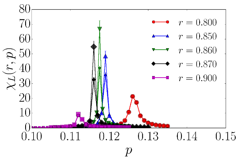
Figure ​​ 11: Coexisting states and fluctuations on a square lattice for $m=1$. (left) Measuring the region of coexisting states by running through a hysteresis-like loop on a square lattice with $N=2048\times 2048$ nodes for fixed $r$ and varying $p$. (right) Fluctuations of the spontaneous recovery model for different fixed values of $r$ and varying $p$. At around $r=0.86(1)$ and $p=0.117(3)$ we find the largest fluctuations corresponding to the bifurcation point. Simulations were performed for $N=128\times 128$ (smaller symbols) and $N=256\times 256$ (larger symbols) nodes (50 samples).

In the square lattice we search for the bifurcation point by first analyzing the hysteresis behavior of the dynamics as shown in Fig. 11 (left). The region where the area defining the multiple states in the hysteresis curve becomes negligible characterizes the vicinity of the cusp point. We then search for the critical point by measuring the fluctuations in that region:

$$\chi_{L}(r,p)=L^{2}\left[\langle a_{st}^{2}\rangle-\langle a_{st}\rangle^{2}\right].$$ (12)

The fluctuations in the vicinity of the bifurcation point are shown in Fig. 11. We conclude that the cusp point where both spinodals meet is located around $(r_{c},p_{c})=(0.86(1),0.117(3))$.

In summary, the arguments in Appendix A and above for the case $m=3$ (analytical and numerical) show the similarities between our model and the (non-equilibrium) contact process belonging to the directed percolation universality class Henkel et al. (2008). Thus, we do not expect the dynamics to belong to the Ising universality class as conjectured in Ref. Majdandzic et al. (2014). As already mentioned in Ref. Grassberger (1982) if this contact process dynamics would belong to the Ising universality class it would mean the extension of the universality hypothesis from models with detailed balance to models without it.

References

- Verma et al. (2016) T. Verma, F. Russmann, N. Araújo, J. Nagler, and H. Herrmann, Nat. Commun. 7, 10441 (2016).
- Barabási et al. (2011) A.-L. Barabási, N. Gulbahce, and J. Loscalzo, Nat. Rev. Genet. 12, 56 (2011).
- Barthélemy (2011) M. Barthélemy, Phys. Rep. 499, 1 (2011).
- Cohen et al. (2000) R. Cohen, K. Erez, D. ben Avraham, and S. Havlin, Phys. Rev. Lett. 85, 4626 (2000).
- Albert et al. (2000) R. Albert, H. Jeong, and A.-L. Barabási, Nature 406, 378 (2000).
- Centola et al. (2005) D. Centola, R. Willer, and M. Macy, Am. J. Sociol. 110, 1009 (2005).
- Buldyrev et al. (2010) S. V. Buldyrev, R. Parshani, G. Paul, H. E. Stanley, and S. Havlin, Nature 464, 1025 (2010).
- Helbing (2013) D. Helbing, Nature 497, 51 (2013).
- Bashan et al. (2013) A. Bashan, Y. Berezin, S. V. Buldyrev, and S. Havlin, Nat. Phys. 9, 667 (2013).
- Coleman et al. (1957) J. Coleman, E. Katz, and H. Menzel, Sociometry 20, 253 (1957).
- Rogers (2010) E. M. Rogers, Diffusion of Innovations (Simon and Schuster, 2010).
- Chwe (1999) M. S. Chwe, Am. J. Sociol. 105, 128 (1999).
- Leskovec et al. (2007) J. Leskovec, L. A. Adamic, and B. A. Huberman, ACM Trans. Web 1 (2007).
- Easley and Kleinberg (2010) D. Easley and J. Kleinberg, Networks, crowds, and markets: Reasoning about a highly connected world (Cambridge University Press, 2010).
- Granovetter (1978) M. Granovetter, Am. J. Sociol. 83, 1420 (1978).
- Centola and Macy (2007) D. Centola and M. Macy, Am. J. Sociol. 113, 702 (2007).
- May et al. (2008) R. M. May, S. A. Levin, and G. Sugihara, Nature 451, 893 (2008).
- Haldane and May (2011) A. G. Haldane and R. M. May, Nature 469, 351 (2011).
- Lorenz et al. (2009) J. Lorenz, S. Battiston, and F. Schweitzer, Eur. Phys. J. B 71, 441 (2009).
- Majdandzic et al. (2014) A. Majdandzic, B. Podobnik, S. V. Buldyrev, D. Y. Kenett, S. Havlin, and H. E. Stanley, Nat. Phys. 10, 34 (2014).
- Achlioptas et al. (2009) D. Achlioptas, R. M. D’Souza, and J. Spencer, Science (2009).
- Araújo and Herrmann (2010) N. A. M. Araújo and H. J. Herrmann, Phys. Rev. Lett. 105, 035701 (2010).
- Nagler et al. (2011) J. Nagler, A. Levina, and M. Timme, Nat. Phys. 7, 265 (2011).
- Nagler et al. (2012) J. Nagler, T. Tiessen, and H. W. Gutch, Phys. Rev. X 2, 031009 (2012).
- Schröder et al. (2013) M. Schröder, S. H. E. Rahbari, and J. Nagler, Nat. Commun. 4, 2222 (2013).
- Cho et al. (2013) Y. S. Cho, S. Hwang, H. J. Herrmann, and B. Kahng, Science (2013).
- Chen et al. (2013a) W. Chen, X. Cheng, Z. Zheng, N. N. Chung, R. M. D’Souza, and J. Nagler, Phys. Rev. E 88, 042152 (2013a).
- Chen et al. (2013b) W. Chen, J. Nagler, X. Cheng, X. Jin, H. Shen, Z. Zheng, and R. M. D’Souza, Phys. Rev. E 87, 052130 (2013b).
- Chen et al. (2014) W. Chen, M. Schröder, R. M. D’Souza, D. Sornette, and J. Nagler, Phys. Rev. Lett. 112, 155701 (2014).
- Böttcher et al. (2015) L. Böttcher, O. Woolley-Meza, N. A. M. Araújo, H. J. Herrmann, and D. Helbing, Sci. Rep. 5, 16571 (2015).
- D’Souza and Nagler (2015) R. M. D’Souza and J. Nagler, Nat. Phys. 11, 531 (2015).
- Böttcher et al. (2016) L. Böttcher, O. Woolley-Meza, E. Goles, D. Helbing, and H. J. Herrmann, Phys. Rev. E 93, 042315 (2016).
- Saberi et al. (2016) A. A. Saberi, S. H. E. Rahbari, H. Dashti-Naserabadi, A. Abbasi, Y. S. Cho, and J. Nagler, Sci. Rep. 6, 21110 (2016).
- Schröder et al. (2016) M. Schröder, W. Chen, and J. Nagler, New J. Phys. 18, 013042 (2016).
- Turalska et al. (2009) M. Turalska, M. Lukovic, B. J. West, and P. Grigolini, Phys. Rev. E 80, 021110 (2009).
- Ditzinger and Haken (1989) T. Ditzinger and H. Haken, Biol. Cybern. 61, 279 (1989).
- Moreno-Bote et al. (2007) R. Moreno-Bote, J. Rinzel, and N. Rubin, J. Neurophysiol. 98, 1125 (2007).
- Atwal (2014) G. S. Atwal, BioRxiv (2014).
- Kesselring et al. (2013) T. A. Kesselring, E. Lascaris, G. Franzese, S. V. Buldyrev, H. J. Herrmann, and H. E. Stanley, J. Chem. Phys. 138, 244506 (2013).
- Ding et al. (2002) F. Ding, N. V. Dokholyan, S. V. Buldyrev, H. E. Stanley, and E. I. Shakhnovich, Biophys. J. 83, 3525 (2002).
- Kim et al. (2002) K.-R. Kim, D. J. Lee, and K. J. Shin, J. Chem. Phys. 117, 2710 (2002).
- Binder and Landau (1984) K. Binder and D. P. Landau, Phys. Rev. B 30, 1477 (1984).
- Bashan et al. (2012) A. Bashan, R. P. Bartsch, Jan. W. Kantelhardt, S. Havlin, and P. C. Ivanov, Nat. Commun. 3, 702 (2012).
- Tomé and de Oliveira (2015) T. Tomé and M. J. de Oliveira, Stochastic Dynamics and Irreversibility (Springer, 2015).
- Ludwig et al. (1978) D. Ludwig, D. D. Jones, and C. S. Holling, J. Anim. Ecol. 47, 315 (1978).
- Zeeman (1979) E. C. Zeeman, Catastrophe theory (Springer, 1979).
- Strogatz (2014) S. H. Strogatz, Nonlinear dynamics and chaos: with applications to physics, biology, chemistry, and engineering (Westview press, 2014).
- Gillespie (1976) D. T. Gillespie, J. Comput. Phys. 22, 403 (1976).
- Gillespie (1977) D. T. Gillespie, J. Phys. Chem. 81, 2340 (1977).
- Watts (2002) D. J. Watts, Proc. Natl. Acad. Sci. 99, 5766 (2002).
- López-Pintado (2008) D. López-Pintado, Game Econ. Behav. 62, 573 (2008).
- Sherrington and Kirkpatrick (1975) D. Sherrington and S. Kirkpatrick, Phys. Rev. Lett. 35, 1792 (1975).
- Kirkpatrick and Sherrington (1978) S. Kirkpatrick and D. Sherrington, Phys. Rev. B 17, 4384 (1978).
- Sornette (2006) D. Sornette, Critical phenomena in natural sciences: chaos, fractals, selforganization and disorder: concepts and tools (Springer Science & Business Media, 2006).
- vid (a) Video 1 (https://vimeo.com/162425603).
- vid (b) Video 2 (https://vimeo.com/162425733).
- vid (c) Video 3 (https://vimeo.com/163988456).
- Danziger et al. (2015) M. M. Danziger, L. M. Shekhtman, Y. Berezin, and S. Havlin, arXiv preprint , arXiv:1505.01688 (2015).
- vid (d) Video 4 (https://vimeo.com/172921549).
- Henkel et al. (2008) M. Henkel, H. Hinrichsen, and S. Lübeck, Non-Equilibrium Phase Transitions Volume I: Absorbing Phase Transitions (Springer, 2008).
- Grassberger (1982) P. Grassberger, Z. Phys. B 47 (1982).
- Marro and Dickman (2005) J. Marro and R. Dickman, Nonequilibrium Phase Transitions in Lattice Models (Cambridge University Press, 2005).
- Vellela and Qian (2009) M. Vellela and H. Qian, J. R. Soc. Interface 6, 925 (2009).
- Moreira and Dickman (1996) A. G. Moreira and R. Dickman, Phys. Rev. E 54, R3090 (1996).
- Adler and Duarte (1987) J. Adler and J. A. M. S. Duarte, Phys. Rev. B 35, 7046 (1987).