Nucleation, instability, and discontinuous phase transitions in monoaxial helimagnets with oblique fields

Abstract

The phase diagram of the monoaxial chiral helimagnet as a function of temperature ($T$) and magnetic field with components perpendicular ($H_{x}$) and parallel ($H_{z}$) to the chiral axis is theoretically studied via the variational mean field approach in the continuum limit. A phase transition surface in the three dimensional thermodynamic space separates a chiral spatially modulated phase from a homogeneous forced ferromagnetic phase. The phase boundary is divided into three parts: two surfaces of second order transitions of instability and nucleation type, in De Gennes terminology, are separated by a surface of first order transitions. Two lines of tricritical points separate the first order surface from the second order surfaces. The divergence of the period of the modulated state on the nucleation transition surface has the logarithmic behavior typical of a chiral soliton lattice. The specific heat diverges on the nucleation surface as a power law with logarithmic corrections, while it shows a finite discontinuity on the other two surfaces. The soliton density curves are described by a universal function of $H_{x}$ if the values of $T$ and $H_{z}$ determine a transition point lying on the nucleation surface; otherwise, they are not universal.

I Introduction

Chiral magnets are currently the subject of intense investigations both because of their practical applications in technology and their interesing properties from the point of view of fundamental science. The applications exploit the charge and spin transport properties of a chiral magnet, which are strongly affected by the magnetic structure and thus can be controlled by the application of suitable magnetic fields Wolf et al. (2013); Žutić et al. (2004). In addition, due to its topological nature, the magnetic structure of a chiral magnet is protected against continuous deformations to homogeneous magnetic states, as ferromagnetic states. The chiral state can only turn into a homogeneous state through phase transitions that take place at definite points of the phase diagram. This robustness makes chiral magnets excelent candidates as the main components of spintronic devices Fert et al. (2013) and, for instance, they are specially suitable as the main components of information storage devices Romming et al. (2001).

Besides the applications, chiral magnets are very interesting objects from a fundamental point of view, as chiral symmetry and its breaking and restoration are ubiquitous phenomena appearing virtually in any domain of science, from elementary particle physics to astrophysics, and including chemistry, biology, and geology Wagniere (2007).

In the monoaxial helimagnet Kishine and Ovchinnikov (2015), the competition between the ferromagnetic (FM) and Dzyaloshinskii–Moriya Dzyaloshinskii (1958); Moriya (1960) (DM) interactions at low $T$ give rise to a spatially modulated chiral magnetic structure that, in absence of an applied field, has the form of an helix propagating with period $L_{0}$ along the chiral axis, which is called here the DM axis. At a certain ordering temperature, $T_{0}$, a magnetic transition to a paramagnetic (PM) phase takes place. The period $L_{0}$ is independent of $T$, but the local magnetic moment decreases with $T$, and the transition to the PM state takes place at the temperature where it vanishes. The nature of the transition at $T_{0}$ is not fully understood and considerable effort is being devoted to clarify this interesting question Tsuruta et al. (2016); Bornstein et al. (2015); Ghimire et al. (2013); Chapman et al. (2014); Shinozaki et al. (2016); Laliena et al. (2016a); Nishikawa and Hukushima (2016).

At temperatures lower than $T_{0}$, application of a magnetic field perpendicular to the DM axis deforms the helix and a chiral soliton lattice (CSL) appears Kishine and Ovchinnikov (2015); Dzyaloshinskii (1958, 1964); Izyumov (1984); Kishine et al. (2005). This CSL, which is realized Togawa et al. (2012) in $\mathrm{CrNb}_{3}\mathrm{S}_{6}$, supports phenomena very interesting for spintronics, like spin motive forces Ovchinnikov et al. (2013) and tuneable magnetoresistence Kishine et al. (2011); Togawa et al. (2013); Ghimire et al. (2013); Bornstein et al. (2015). A theoretical analysis at zero temperature carried out long ago Dzyaloshinskii (1964) concluded that by increasing the field the period of the CSL increases and, eventually, as the period diverges, a phase transition takes place continuously to a forced FM (FFM) state. This prediction has been recently confirmed experimentally Togawa et al. (2012, 2013) and theoretically by computations at finite temperature Laliena et al. (2016a).

If, on the other hand, the applied field is parallel to the DM axis, the local magnetic moment acquires a constant component along the axis and a conical helix is formed. The conical helix propagates with a period $L_{0}$ which is independent of temperature and field intensity. As the field increases, the component of the local magnetic moment parallel to the DM axis increases and the perpendicular component decreases. A transition to a homogeneous FFM state takes place when the perpendicular component vanishes. The same happens if the temperature is increased at constant parallel field.

A classification of the continuous transitions that take place between spatially homogeneous and modulated states was introduced long ago by DeGennes de Gennes , who called nucleation transitions those in which the period of the modulated state diverges when the transition point is approached from the modulated phase, and instability transitions those in which the phase transition takes place when the intensity of the Fourier modes with non-zero wave vector tend to zero, while the fundamental wavevector remains finite and does not vanish. The mechanisms for these two kind of transitions are qualitatively different. In the monoaxial helimagnet, the transition between the CSL and the FFM states as a perpendicular magnetic field increases at sufficiently low temperature is of nucleation type Dzyaloshinskii (1964); Laliena et al. (2016a). On the other hand, at zero field mean field theory predicts an instability type continuous transition at the ordering temperature $T_{0}$. The transition to the FFM in presence of a parallel magnetic field is also of second order instability type phase transition.

Hence, by varying the temperature from $0$ to $T_{0}$ and/or the applied field from completely perpendicular to completely parallel, the transition changes from nucleation to instability type. How this change of regime takes place is a very interesting question which may also have interesting phenomenological consequences.

Recently, the zero temperature phase diagram of the monoaxial helimagnet has been theoretically analized for oblique magnetic fields Laliena et al. (2016b), which are neither perpendicular nor parallel to the DM axis. It has been found that in the thermodynamic space formed by the parallel and perpendicular components of the magnetic field two separated continuous transition lines appear. The transitions along the line that contains as limiting case the parallel field are of instability type and the transitions along the other line, which contains as limiting case the perpendicular field, are of nucleation type. The two continuous lines are separated by a line of discontinuous transitions. Two tricritical points separate the discontinuous transition line from the continuous transition lines.

Also recently the phase diagram of the monoaxial helimagnet in the thermodynamic space defined by the temperature and a perpendicular magnetic field has been theoretically studied in Ref. Laliena et al., 2016a. The conclusion is that at low $T$ the transitions to the FFM state induced by the perpendicular field are continuos, of nucleation type, with the period of the chiral structure diverging at the transition points. As temperature increases the critical field decreases and vanishes at the zero field critical temperature, $T_{0}$. The transition at $T_{0}$ is continuous of instability type. The transition line in the vicinity of $T_{0}$ is of first order and it is separated from the low $T$ continuous transition line by a tricritical point. This somehow unexpected behavior is rather logical as it is difficult to imagine how to connect continuously instability and nucleation transitions. The prediction of a first order transition and a tricritical point in the vicinity of $T_{0}$ may be a clue to the interpretation of the experimental results on the phase diagram reported in Refs. Tsuruta et al., 2016; Bornstein et al., 2015; Ghimire et al., 2013. A more refined numerical computation around the $T_{0}$ neighborhood, carried out in this work, leads to the conclusion that the first order line does not actually end at $T_{0}$, but instead the transition is of second order instability type in a very short line that ends at $T_{0}$. Correspondingly, a second tricritical point appears separating this short second order line from the first order line. This tricritical point was unnoticed in Ref. Laliena et al., 2016a.

In this work we complete the theoretical study of the phase diagram of the monoaxial helimagnet and the nature of its phase boundaries by analyzing it in the 3D thermodynamic space $H_{x}-H_{z}-T$, where $H_{x}$ and $H_{z}$ stand repectively for the perpendicular and parallel components of the magnetic field. The thermal fluctuations are treated classically and therefore the results are not valid at very low T, where it is well known that a quantum treatment of thermal fluctuations is necessary, for instance, to reproduce the behavior of the specific heat. In the zero temperature limit, however, thermal fluctuations disappear and the semiclassical approximation seems to describe well the ground state of these kind of systems.

The methods presented in this work can be applied to other systems in which phase transitions from spatially modulated phases to homegeneous phases take place, as for instance cholesteric liquid crystals.

II Model

Let us consider the model described in Ref Laliena et al., 2016a: a classical spin system with FM exchange and monoaxial DM interactions, and single-ion easy-plane anisotropy, at temperature $T$ and in presence of an applied magnetic field $\vec{H}$. In what follows we use the notation of Ref. Laliena et al., 2016a, and take the $\hat{z}$ coordinate axis along the DM axis.

To get the thermodynamical properties we evaluate the free energy, $\mathcal{F}$, through the variational mean field approximation, which has been succesfully applied to the study of the double-exchange model of itinerant ferromagnetism Alonso et al. (2001a, b, 2002) and, in combination with ab-initio techniques, to the study of the temperature dependence of thermodynamic quantities in itinerant ferromagnetsGyorffy et al. (1985); Staunton et al. (1986, 2006). The free energy is obtained by minimizing the mean field free energy, $\mathcal{F}_{0}$, with respect to the mean field configuration, $\vec{M}_{\vec{r}}$. In the continuum limit, taken along the lines described in Ref. Laliena et al., 2016a, we get $\mathcal{F}_{0}=\epsilon_{0}\int d^{3}rf_{0}(\vec{r})$, with

$$f_{0}=\frac{1}{2}\sum_{i}\xi_{i}(\partial_{i}\vec{m})^{2}-q_{0}\hat{z}\cdot(\vec{m}\times\partial_{z}\vec{m})-q_{0}^{2}(\vec{h}\cdot\vec{m}+U),$$ (1)

where

$$U=\frac{\mu^{2}}{2}m^{2}-\gamma\left[F+(1-3F)\frac{m_{z}^{2}}{m^{2}}\right]+\alpha\left[\ln\frac{\sinh M}{M}-Mm\right],$$ (2)

where $\vec{m}=F\vec{M}$ is the mean local magnetic moment and $F=\coth(M)/M-1/M^{2}$,

The relation of the parameters entering Eqs. (1) and (2) with a more fundamental Hamiltonian is given in Ref. Laliena et al., 2016a. The $\xi_{i}$ measure the spatial anisotropy of the FM exchange couplings. By definition, $\xi_{z}=1$, and in this work we consider only system of symmetry such that $\xi_{x}=\xi_{y}=\xi$. The parameter $q_{0}$ has dimensions of inverse length and gives the propagation vector of the helical modulation at zero field. The remaining parameters are dimensionless: $\mu^{2}$ controls the continuum limit and has to be large Laliena et al. (2016a); and $\gamma$, $\alpha$, and $\vec{h}$ are proportional to the single-ion anisotropy, temperature ($T$) and external magnetic field ($\vec{H}$), respectively. Finally, $\epsilon_{0}$ is an overall constant with the dimensions of energy per unit length. All these parameters might be obtained from ab-initio calculations, but in practice can be fit to experimental results to describe the phase diagram of different samples and materials.

III Method of solution

The minimum of $\mathcal{F}_{0}$ is a solution of the corresponding Euler-Lagrange equations. Clearly, the mean field configuration which minimizes $\mathcal{F}_{0}$ depends only on $z$ and the equations read

$$\vec{M}^{\prime\prime}=\Omega\vec{M}^{\prime}+2q_{0}\hat{z}\times\vec{M}^{\prime}+\Psi\vec{M}+\Upsilon\hat{z}\times\vec{M}+\Pi M_{z}\hat{z}-q_{0}^{2}\vec{h}/F.$$ (3)

The scalar functions $\Omega$, $\Psi$, $\Upsilon$, and $\Pi$ depend on $\vec{M}$ and $\vec{M}^{\prime}$. They are given in appendix A.

Equations (3) constitute a system of three second order differential equations, the general solution of which contains six arbitrary integration constants. The task is to find the particular solution which minimises $\mathcal{F}_{0}$. We follow the method described in Ref. Laliena et al., 2016b. On physical grounds, we expect a periodic ground state, with period $L$. Hence, the free energy density $\bar{f}_{0}=\mathcal{F}_{0}/V$, where $V$ is the volume, is equal to the free energy averaged over one period, that is $\bar{f}_{0}=(1/L)\int_{0}^{L}f_{0}(z)dz$, and the boundary conditions (BC) are $\vec{M}(0)=\vec{M}(L)$. Since the equations are of second order, these BC do not guarantee periodicity, which requires also the equality of the first derivatives at the two boundaries: $\vec{M}^{\prime}(0)=\vec{M}^{\prime}(L)$. These additional conditions cannot be generally imposed on the boundary value problem (BVP), since it would be overdetermined. The strategy to find a solution to the problem is as follows: with no loss, set $M_{y}(0)=M_{y}(L)=0$, and for given $L$ and $M_{x}(0)=M_{x0}$, and $M_{z}(0)=M_{z0}$, solve numerically the BVP; for fixed $L$, tune $M_{x0}$ and $M_{z0}$ until periodicity is reached; then, compute $\bar{f}_{0}$ via a numerical quadrature algorithm. The equilibrium period is the minimum of $\bar{f}_{0}$, which is found via a simple minimisation algorithm.

IV Phase diagram

Without any loss, we can choose a magnetic field with components along $\hat{x}$ and $\hat{z}$, and set $h_{y}=0$. Two phases appear: the homogeneous FFM state at high temperature and/or high field and a spatially modulated structure at low temperature and low field, which is generically named here helicoid.

A surface of phase transitions in the thermodynamic space $(T,H_{x},H_{z})$ separates the helicoid and FFM phases. The transition surface can be described by giving one of the thermodynamic coordinates as a function of the other two. The dependent coordinate is denoted by $T_{c}$, or $H_{xc}$, or $H_{zc}$.

The transition points on the three axes of the thermodynamic space can be analytically obtained: the critical temperature at zero field, $\alpha_{0}$, and the critical perpendicular and parallel fields at zero temperature, $h_{x0}$ and $h_{z0}$, respectively. Their analytic expressions are:

$$\alpha_{0}=\frac{1}{3}(\mu^{2}+1)+\frac{2}{15}\gamma,\quad h_{x0}=\frac{\pi^{2}}{16},\quad h_{z0}=1+2\gamma.$$ (4)

The corresponding dimensionfull quantities, denoted by $T_{0}$, $H_{x0}$, and $H_{z0}$, are directly measurable quantities: zero field critical temperature and zero temperature critical perpendicular and parallel fields, respectively. It is convenient to present the results in terms of $T/T_{0}=\alpha/\alpha_{0}$, $H_{x}/H_{x0}=h_{x}/h_{x0}$, and $H_{z}/H_{z0}=h_{z}/h_{z0}$. We also use the notation $H_{0}=\sqrt{H_{x0}^{2}+H_{z0}^{2}}$, and denote by $\theta$ the angle formed by the magnetic field and the DM axis: $\tan\theta=H_{x}/H_{z}$. Except in the $H_{z}=0$ separate discussion given below, all the results presented here correspond to $\mu^{2}=210$, which is a value appropriate to describe the phenomenology of $\mathrm{CrNb}_{3}\mathrm{S}_{6}$Laliena et al. (2016a).

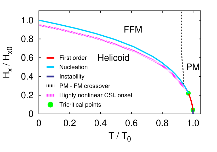
Figure 1: $H_{x}-T$ phase diagram for $H_{z}=0$ (perpendicular field) calculated with $\mu^{2}=120$ and $\gamma=2.58$. The light and dark blue lines correspond to second order nucleation and instability type transitions, respectively, and the red line to first order transitions. The pink dotted line marks the onset of the highly nonlinear CSL. The dashed black line signals the crossover from PM to FM behavior. The tricritical point closer to $T_{0}$ was unnoticed in Ref. Laliena et al., 2016a.

For $H_{z}=0$ we have re-analyzed the transition line in the very close neighborhood of the zero field transition with more detail and accuracy than in Ref. Laliena et al., 2016a. In this region there is instability caused by the critical fluctuations and the numerical computations are more difficult. It turns out that a second tricritical point, not detected in Ref. Laliena et al., 2016a, appears at $T/T_{0}\approx 0.9989$ and $H_{x}/H_{x0}\approx 0.027$. Hence, the transition line is of second order nucleation type at low temperature and of second order instability type at high temperature. These two second order lines are separated by a first order line, and two tricritical points separate the first order line from the second order lines. The phase diagram is displayed in Fig. 1. Notice the slight difference with the phase diagram published in Ref. Laliena et al., 2016a. Although the region around the zero field phase transition, in which the fluctuations are expected to be strongly correlated, is probably not well described by mean field theory, these results give a hint on what can be expected, before more sophisticated approaches, like Monte Carlo simulations, are fully developed. Work in this direction has been reported in Ref. Nishikawa and Hukushima, 2016.

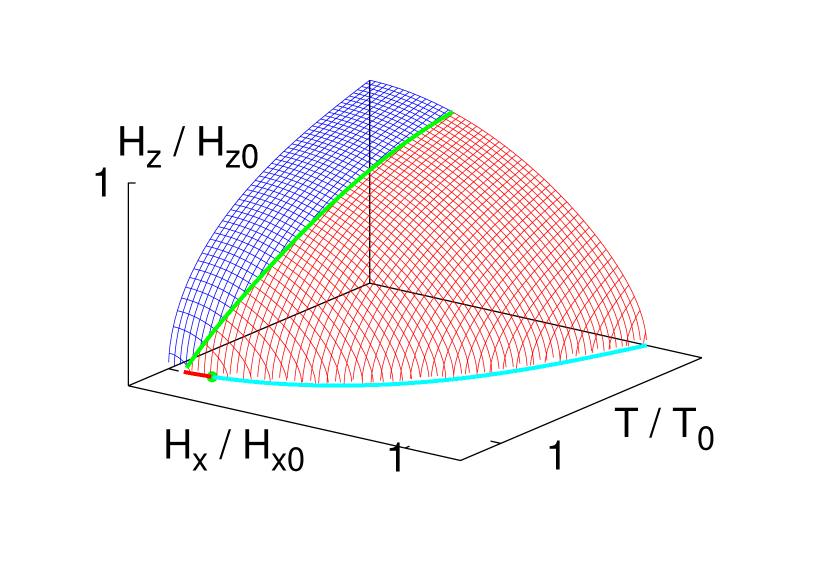
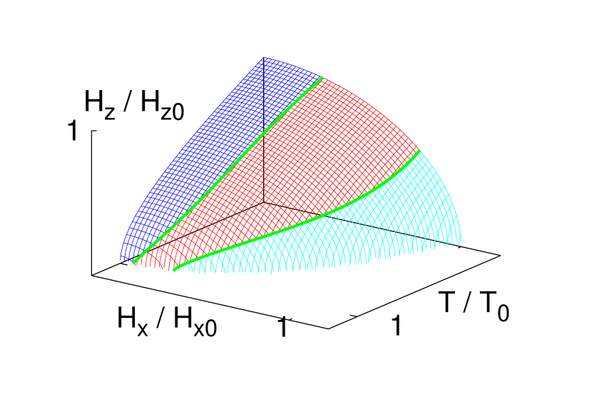
Figure 2: 3D phase diagram without (top) and with (bottom) single-ion anisotropy ($\gamma=2.58$). The second order transitions take place on the dark blue (instability) and light blue (nucleation) portions of the transition surface. On the red portion the transitions are of first order. The tricritical lines separating the first order surface from the two second order surfaces are displayed in green.

For $H_{x}=0$ the free energy is minimized by a conical helix with pitch $L_{0}$ independent of $\alpha$ and $h_{z}$. The angle $\theta_{0}$ which forms $\vec{m}$ with the DM axis depends on temperature and magnetic field. The transition to the FFM state takes place continuously as $\cos\theta_{0}\rightarrow 1$ and is of instability type. An order parameter which vanishes in the FFM state is $\sin\theta_{0}$. As the transition line is approached $\sin\theta_{0}$ vanishes as a power law, with the mean field exponent: $\sin\theta_{0}\sim(1-\alpha/\alpha_{c})^{1/2}$ or $\sin\theta_{0}\sim(1-h_{z}/h_{zc})^{1/2}$.

Three dimensional representations of the phase diagram without ($\gamma=0$) and with ($\gamma=2.58$) anisotropy are displayed on the top and botom panels of Fig. 2, respectively. The value $\gamma=2.58$ has been chosen so that the critical parallel field of $\mathrm{CrNb}_{3}\mathrm{S}_{6}$ at relatively low $T$ is reproduced Laliena et al. (2016b).

Let us discuss first the general case with non vanishing anisotropy. The transition surface is divided into three parts: two surfaces of second order transitions are separated by a surface of first order transitions. The second order transitions of the surface that intersects the $H_{x}=0$ plane are of instability type, while the transitions of the other second order surface are of nucleation type. The instability surface is separated from the first order surface by a line of tricritical points that is called the instability tricritical line (ITC). Analogously, the boundary between the nucleation and the first order surfaces is a line of tricritical points called the nucleation tricritical line (NTC). The tricritical points TC_I and TC_N found at $T=0$ in Ref. Laliena et al., 2016b belong to ITC and NTC, respectively.

As $\gamma\rightarrow 0$ the nucleation surface shrinks and in the absence of single-ion anisotropy (Fig. 2, top) is squeezed onto a line on the $H_{z}=0$ plane. The transition surface contains a second order instability surface and a first order surface separated by the ITC line. The NTC line is reduced to a point on the $H_{z}=0$ plane.

In terms of $T/T_{0}$, $H_{x}/H_{x0}$, and $H_{z}/H_{z0}$, the shape of the transition surface is nearly independent of $\mu^{2}$ provided that $\mu^{2}$ is large enough. It depends, however, on the value of the single-ion anisotropy, although this dependence disappears gradually as the anisotropy grows; in this case it shows noticeably dependence on $\gamma$ only for $T$ close to $T_{0}$. This dependence is related to the fluctuations of $m_{z}^{2}$ at high $T$.

The structure of the modulated state depends on temperature and magnetic field. For fields with small perpendicular component, it is a slightly distorted conical helix, a quasilinear structure to which only a few Fourier harmonics give a noticeably contribution. As the perpendicular component is gradually increased, higher order Fourier harmonics appear and the helix becomes a conical CSL. A highly nonlinear CSL, receiving appreciably contributions from many Fourier harmonics, appears only in the vicinity of the nucleation surface, in complete similarity with the $H_{z}=0$ case Laliena et al. (2016a). The highly nonlinear CSL regime is not sharply defined, but separated from the rest of the modulated phase by a crossover surface very close to the nucleation surface. This crossover surface is not shown in Fig. 2, but its intersection with the $H_{z}=0$ plane is shown in Fig. 1 (highly nonlinear CSL onset line).

V Singularities on the transition surface

On the first order transition surface the helicoid and FFM states coexist. On both sides of the transition surface the two states are present, one as stable and the other as metastable state. As a consequence of the different entropies of these two states, a latent heat accompanies the transition. The latent heat vanishes on the boundaries of the first order surface (the tricritical lines) and thus reaches a maximum at an interior point of each isothermal transition line, as can be seen in Fig. 3. By increasing $T$ the latent heat maximum increases and its position is shifted towards smaller values of $H_{x}$ and $H_{z}$. The absolute maximum, reached at $H_{z}=0$, is about $3\times 10^{-3}\,k_{\mathrm{B}}T_{0}$ per magnetic ion, what amounts to 6 J/kg in the case of $\mathrm{CrNb}_{3}\mathrm{S}_{6}$($T_{0}\approx 125$ K). Fig. 4 displays the latent heat as a function of $T/T_{0}$ for $H_{z}=0$. Notice the slight difference with the analogous figure of Ref. Laliena et al., 2016a, due to the refined computations in the vicinity of $T_{0}$.

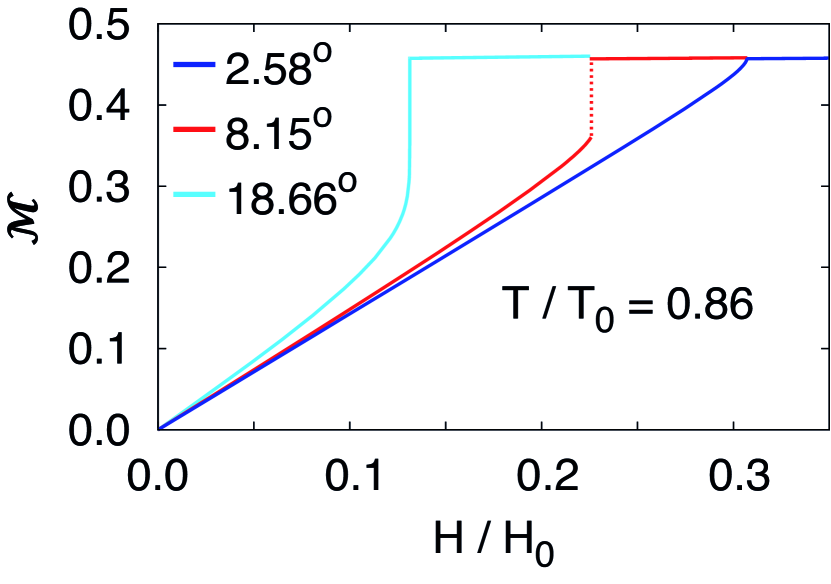
Figure 5: Magnetization per magnetic ion as a function of the field strength for three directions of the field and $T/T_{0}=0.86$. The legend shows the corresponding value of the angle ($\theta$) between the field and the DM axis. The transitions are of second order instability type (dark blue), of first order (red), and of second order nucleation type (light blue). Parameters: $\mu^{2}=210$ and $\gamma=2.58$.

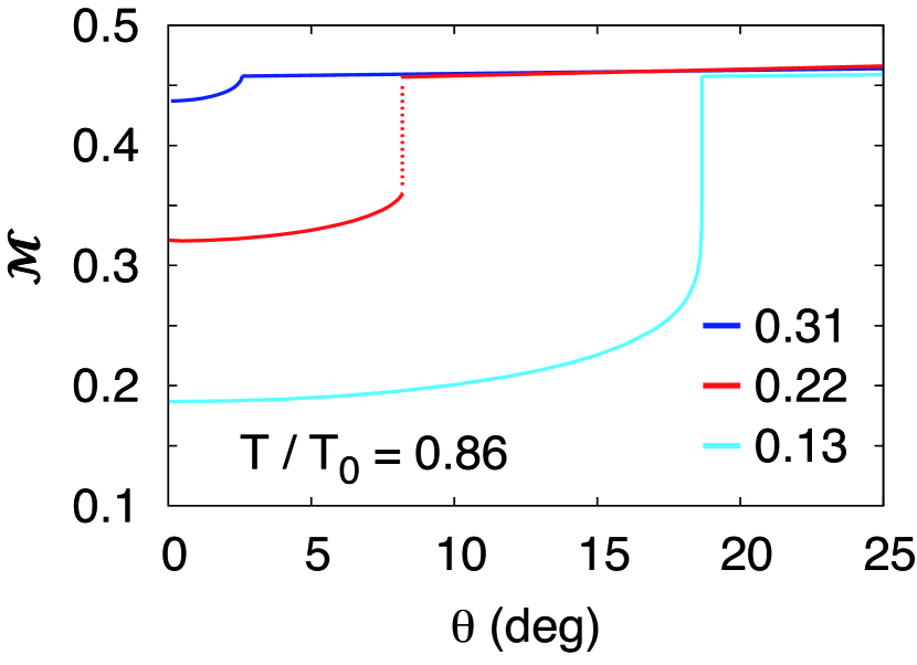
Figure 6: Magnetization per magnetic ion as a function of the angle ($\theta$) between the field and the DM axis, for three field strengths and $T/T_{0}=0.86$. The legend shows the corresponding values of $H/H_{0}$. The transitions are of second order instability type (dark blue), of first order (red), and of second order nucleation type (light blue). Parameters: $\mu^{2}=210$, $\gamma=2.58$.

Fig. 5 displays the behavior of the magnetization per magnetic ion, $\mathcal{M}=(1/L)|\int_{0}^{L}\vec{m}(z)dz|$, as a function of the field strength for three fixed field directions, corresponding to phase transitions of instability type (dark blue), of first order (red), and of nucleation type (light blue). Fig. 6 shows $\mathcal{M}$ versus the field direction at constant field strength, for three values of the field strength that are representative of instability (dark blue), first order (red), and nucleation (light blue) phase transitions. The field direction is characterized by the angle $\theta$ that forms with the DM axis.

On the transition surface $\mathcal{M}$ is singular. It presents a finite discontinuity, signaled by the broken line in Figs. 5 and 6, on the first order surface. On the two second order surfaces $\mathcal{M}$ is continuous, but attains the value of the FFM magnetization in a singular way. On the instability surface the singularity is not very sharp, and, numerically, it seems to be described by a power law, with a critical exponent between 1/2 and 2/3.

The singularity on the nucleation surface is controlled by the divergence of the period, $L$, since the difference between the CSL and FFM magnetization scales as $1/L$. An analysis of the numerical results shows that when the transition point is approached by tuning a parameter $\zeta$, the period $L$ satisfies the scaling law

$$B(Aq_{0}L+1)\exp(-Aq_{0}L)\sim(\zeta_{c}-\zeta)/\zeta_{c},$$ (5)

where $\zeta$ can be either $T$, or $H_{x}$, or $H_{z}$, or $H$, or $\theta$. It is motivated by the well known logarithmic singularity Dzyaloshinskii (1964) that appears as $H_{x}\rightarrow H_{x0}$ at $T=0$ and $H_{z}=0$. Laliena et al. (2016b, a) The scaling of $L$ (and therefore of $\mathcal{M}$) is thus a universal feature of the CSL. It is interesting that the coefficient $A$ depends only on the transition point, and not on the parameter $\zeta$ tuned to reach it.

The inverse of the period, $1/L$, is the density of solitons. It was shown in Ref. Laliena et al., 2016a that for a purely perpendicular field the density of solitons is a universal function of $H_{x}/H_{xc}$, independent of $T$, for temperatures below the nucleation tricritical temperature. Above this tricritical temperature, universality is lost. This universality also holds when the field has a component along the DM axis, provided that the transition point reached by increasing $H_{x}$ while $T$ and $H_{z}$ are kept constant lies on the nucleation surface. It is obvious that the universality cannot hold in the whole phase diagram since in the vicinity of the instability surface $L$ is almost independent of the field. Therefore, the lost of universality is a way of locating the nucleation tricritical line.

The universality of the magnetoresistance curves of $\mathrm{CrNb}_{3}\mathrm{S}_{6}$ in presence of a perpendicular field reported in Ref. Togawa et al., 2013 was linked to the universality of the soliton density curves. Measurements of the magnetorresistance with oblique fields can be used to verify experimentally the universality predicted in the present paper and to locate the nucleation tricritical line of $\mathrm{CrNb}_{3}\mathrm{S}_{6}$.

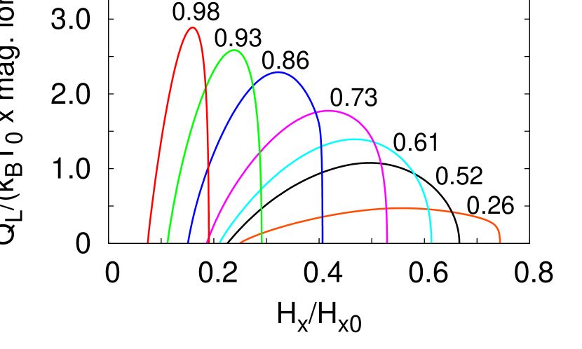
Figure 3: Latent heat per magnetic ion, in units of $k_{\mathrm{B}}T_{0}$, along the first order isothermal transition lines for $T/T_{0}$ indicated in the plot. Parameters: $\mu^{2}=210$ and $\gamma=2.58$.

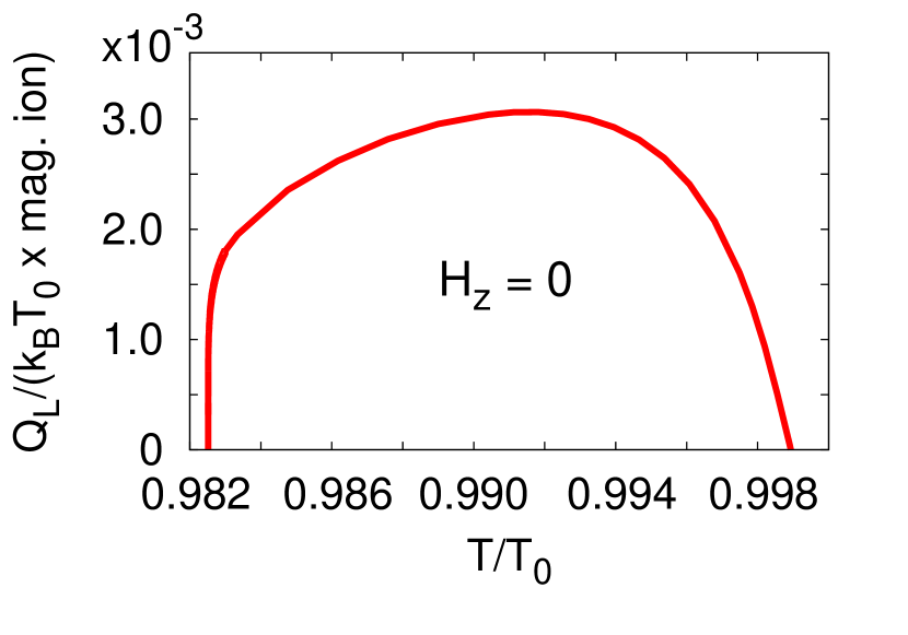
Figure 4: Latent heat per magnetic ion, in units of $k_{\mathrm{B}}T_{0}$, as a function of temperature along the first order transition line for perpendicular field ($H_{z}=0$). It vanishes before reaching $T_{0}$, at a tricritical point in the close vicinity of $T_{0}$, not detected in Ref. Laliena et al., 2016a. Parameters: $\mu^{2}=210$ and $\gamma=2.58$.

VI Specific heat

The specific heat can be computed as $C_{\mathrm{V}}=T\partial s/\partial T$, where $s$ is the specific entropy (per unit mass), which, in the mean field approach, is given by

$$s=\frac{k_{\mathrm{B}}}{\rho v}\frac{1}{L}\int_{0}^{L}\left[\ln(\sinh M/M)-FM^{2}\right]dz,$$ (6)

where $\rho$ is the mass density and $v$ the volume of the unit cell of the underlying lattice and $\vec{M}(z)$ is the equilibrium mean field configuration (i.e., the solution of the Euler-Lagrange equations that minimizes the free energy). This configuration depends in principle on three parameters, the period $L$ and the two BCs, $M_{x0}$ and $M_{z0}$. However, as discussed in section III, only one of these three parameters can be independently chosen. For a given value of $L$, the two BCs are determined by the requirement of periodicity. Hence, $\vec{M}$ is a function of $z$ and $L$, which in its turn is a function of the temperature and the field. As a result, all the $T$ dependence of $s$ comes from its $L$ dependence. Hence we have

$$C_{\mathrm{V}}=\frac{\partial s}{\partial L}T\frac{\partial L}{\partial T}$$ (7)

On the nucleation surface $T\partial L/\partial T$ diverges. From Eq. (5), with $\zeta=T$, we get that for $T\rightarrow T_{c}$

$$T\frac{\partial L}{\partial T}\sim\frac{1}{A}\frac{T_{c}}{T_{c}-T}.$$ (8)

An expression for the factor $\partial s/\partial L$ can be readily obtained from (6):

$$\frac{\partial s}{\partial L} = \frac{k_{\mathrm{B}}}{\rho v}\frac{1}{L}\int_{0}^{L}GM\frac{\partial M}{\partial L}dz$$ (9)

$$+ \frac{1}{L}\left\{\frac{k_{\mathrm{B}}}{\rho v}\left[\ln(\sinh M_{0}/M_{0})-FM_{0}^{2}\right]-s\right\},$$

where $M_{0}=\sqrt{M_{x0}^{2}+M_{z0}^{2}}$ is the value of $M$ at the boundaries $z=0$ and $z=L$, and we used the fact that the derivative with respect to $M$ of the integrand of Eq. (6) is $GM$, with $G=F+MdF/dM$.

In the $T\rightarrow T_{c}$ limit $M$ and $M_{0}$ tend to the FFM mean field as $1/L$. Thus, the two terms of the right hand side of Eq. (9) vanish as $1/L^{2}$ (the term in curly braces tends to the difference of the CSL and FFM specific entropies and thus vanishes as $1/L$). This simply means that, since $s$ tends to the FFM entropy as $1/L$, its derivative with respect to $L$ vanishes as $1/L^{2}$. Thus, taking into account that $L\sim\ln(T_{c}-T)$, the specific heat diverges on the nucleation surface as

$$C_{\mathrm{V}}\sim 1/[(T_{c}-T)\ln^{2}(T_{c}-T)].$$ (10)

The numerical computations confirm this behavior. A fit of the parameters $c_{0}$ and $b$ of the function

$$c_{0}/[(1-T/T_{c})\ln^{b}(1-T/T_{c})]$$ (11)

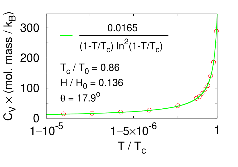
Figure 7: Divergence of the specific heat as a nucleation transition point is approached. The legend displays the value of the field, which is kept fixed, and of the transition temperature. Parameters: $\mu^{2}=210$ and $\gamma=2.58$.

to the computed $C_{\mathrm{V}}$ for fixed field in the region close to $T_{c}$ gives $b=2.08\pm 0.078$, which is perfectly compatible with $b=2$. Therefore, we may fix $b=2$ and fit the single parameter $c_{0}$. The result is displayed in Fig 7. We observe a perfect agreement of the numerical results with the theoretical expectation. The divergence of the specific heat found here is remarkable since in the “canonical” mean field theory of the PM-FM transition the specific heat has no divergence, but shows a finite discontinuity at the critical point.

On the first order surface the specific heat has obviously a finite discontinuity. It shows also a finite discontinuity on the instability surface, since $L$ and its derivatives remain finite there. For zero field, the specific heat jump at $T=T_{0}$ can be analytically computed as follows. The low $T$ ground state is an helix with pitch $L_{0}$ and $M(z)=M_{0}$ independent of $z$, determined by

$$(\mu^{2}+1)F(M_{0})-\gamma F_{1}(M_{0})/[M_{0}G(M_{0})]=\alpha.$$ (12)

The left hand side of the above equation attains its maximum value at $M_{0}=0$, which gives $\alpha_{0}$ defined in Eq. (4). Thus, for $\alpha>\alpha_{0}$ Eq. (12) has no solution and the system is in the PM phase. The solution of (12) decreases monotonically with $\alpha$ from $M_{0}=\infty$ (what implies saturation of magnetization, $m=1$) at $\alpha=0$ to $M_{0}=0$ at the critical point $\alpha_{0}$. The transition to the PM phase at $\alpha_{0}$ takes place continuously and $M_{0}$ vanishes as a power law: $M_{0}\sim(1-T/T_{0})^{1/2}$. It is a second order instability type transition. The specific entropy is given by

$$s=\frac{k_{\mathrm{B}}}{\rho v}\left[\ln(\sinh M_{0}/M_{0})-FM_{0}^{2}\right],$$ (13)

and the specific heat by

$$C_{\mathrm{V}}=\frac{k_{\mathrm{B}}}{\rho v}GM_{0}\alpha\frac{\partial M_{0}}{\partial\alpha}.$$ (14)

Implicit differenciation of Eq. (12) with respect to $\alpha$ gives

$$\frac{\partial M_{0}}{\partial\alpha}=\frac{G^{2}M_{0}^{2}/F_{1}}{1+\mu^{2}+\gamma\left(F+3M_{0}F_{1}+M_{0}^{2}F_{2}-GF_{2}M_{0}/F_{1}\right)}.$$ (15)

For $T\rightarrow T_{0}$ (i.e. $\alpha\rightarrow\alpha_{0}$) we have $M_{0}\rightarrow 0$, and to leading order in $1/M_{0}$ the above equation gives

$$\frac{\partial M_{0}}{\partial\alpha}\sim\frac{45/2}{1+\mu^{2}+(2/35)\gamma}\frac{1}{M_{0}},$$ (16)

so that

$$C_{\mathrm{V}}=\frac{k_{\mathrm{B}}}{\rho v}\frac{5}{2}\left[\frac{\mu^{2}+1+(2/5)\gamma}{\mu^{2}+1+(2/35)\gamma}+O(T_{0}-T)\right],$$ (17)

where we have substituted $G$ by 1/3, which is its value at $M=0$, and $\alpha$ by the value $\alpha_{0}$ given by Eq. (4). In the PM phase mean field theory gives $M_{0}=0$, $s=0$, and $C_{\mathrm{V}}=0$, and therefore the specific heat jump at the zero field critical point is given by Eq. (17). Since $\mu^{2}\gg 1$, the specific heat jump is nearly independent of $\mu^{2}$ and $\gamma$, and is given by $\Delta C_{\mathrm{V}}\approx(5/2)k_{\mathrm{B}}/\rho v$.

The behavior of the specific heat as a function of $T/T_{0}$ for fixed field is displayed in Fig. 8 for the three values of the field shown in the legend. In the three cases the transition temperature is the same, $T_{c}/T_{0}=0.862$. The phase transitions are of instability type (dark blue), of first order (red), and of nucleation type (light blue). In the helicoid phase the specific heat is basically independent of the field, except in the close vicinity of the phase transition, where it shows a rapid growth in the case of the second order transitions of both types. However, as can be appreciated in the inset of Fig. 8, which shows the behavior of $C_{\mathrm{V}}$ around $T_{C}$, the specific heat diverges in the case of the nucleation transition but remains finite in the instability case.

In the low field case (light blue line), the specific heat presents a broad shoulder in the high temperature phase that is associated to the crossover from PM to FFM behavior. This defines a crossover surface in the 3D phase diagram, which is not shown in Fig. 2. Its intersetion with the $H_{z}=0$ plane, however, is shown in Fig. 1.

VII Summary and conclusion

A complete characterization of the phase diagram of the monoaxial helimagnet in the presence of a magnetic field with components parallel and perpendicular to the DM axis has been obtained by means of the variational mean field approach. The phase diagram contains a low-field and low-temperature phase in which the ground state is a spatially modulated chiral magnetic structure and a high-field/high-T phase in which the system is in a homogeneous forced ferromagnetic state (paramagnetic at zero field and high temperature). The phase boundary is a surface in the three dimensional thermodynamic space defined by the temperature and the parallel and perpendicular components of the magnetic field. The transition surface is divided into three parts: one surface of first order transitions separates two surfaces of second order transitions, in one of which the transitions are of instability type and in the other one of nucleation type. The first order surface is separated from the second order surfaces by two lines of tricritical points.

It is worthwhile to recall that mean field theory, which approximates the thermal fluctuations by the uncorrelated fluctuations of the trial “Hamiltonian”, usually fails in the critical domain, where the fluctuations are strongly correlated. In our case, except for a small neighborhood of the zero field transition, the fluctuations are not expected to be critical, since the transitions are driven by the magnetic field, and the computations should be accurate, or at least qualitatively correct. Only in the vicinity of the zero field phase transition, where critical fluctuations are expected, mean field theory may fail, and other techniques, as Monte Carlo simulations, are necessary to validate or disproof the mean field results.

The period of the modulated state diverges on the nucleation surface. The divergence obeys a logarithmic scaling law, Eq. (5), which is a distinct feature of the CSL. It induces a singularity in the magnetization also characteristic of the CSL. The specific heat is also divergent on the nucleation surface, with a scaling law that has the form of a power law with logarithmic corrections. This is remarkable since in the “canonical” mean field theory of the FM-PM transition the specific heat does not diverge, but shows a finite discontinuity.

The soliton density is a universal function of the reduced perpendicular component of the field, $H_{x}/H_{xc}$. Universality means independence of the temperature and of the parallel component of the field, and holds only if the transition point obtained by tuning $H_{x}$, keeping fixed $T$ and $H_{z}$, lies on the nucleation surface. Otherwise, universality is lost. Thus, this universality can be used to locate the tricritical line that separates the first order surface from the nucleation surface.

The picture that emerge from this work should serve to stimulate the experimental study of the magnetic properties of compounds like $\mathrm{CrNb}_{3}\mathrm{S}_{6}$, and to interpret some of the already known and forthcoming experimental data. For instance, the phase diagram in the immediate vicinity of the zero field ordering transition has a complex structure, with first and second order transitions separated by a tricritical point, and deserves a thorough experimental investigation.

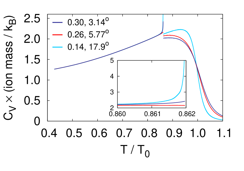
Figure 8: Specific heat vs. $T/T_{0}$ for three fixed values of the field specified in the legend, in polar coordinates ($H/H_{0}$, $\theta$). In the three cases the phase transition takes place at $T_{c}/T_{0}=0.862$ and are of second order instability type (dark blue), of first order (red), and of second order nucleation type (light blue). The inset displays the behavior in the vicinity of the transition. Parameters: $\mu^{2}=210$ and $\gamma=2.58$.

Appendix A Some details about the Euler-Lagrange equations

In this appendix we give some details about the derivation of the Euler-Lagrange equations, Eq. (3). On physical grounds, the minimum of $\mathcal{F}_{0}=\epsilon_{0}\int d^{3}rf_{0}(\vec{r})$, with $f_{0}$ given by Eq. (1), is a function of the coordinate $z$ along the DM axis only. Hence, in the search for the minimum we can restrict the functional to mean field configurations that depend only on $z$, and the functional reads $\mathcal{F}_{0}=A\epsilon_{0}\int dzf_{0}(z)$, where $A=\int dxdy$ is the area of the sample cross section perpendicular to the DM axis and

$$f_{0}(z)=\frac{1}{2}\vec{m}^{\prime\,2}-q_{0}\hat{z}\cdot(\vec{m}\times\vec{m}^{\prime})-q_{0}^{2}(\vec{h}\cdot\vec{m}+U),$$ (18)

where the prime stands for the derivative with respect to $z$ and $U$ is given by Eq. (2). The Euler-Lagrange equations then read

$$\frac{d}{dz}\frac{\partial f_{0}}{\partial M_{i}^{\prime}}-\frac{\partial f_{0}}{\partial M_{i}}=0$$ (19)

for $i\in\{x,y,z\}$. Since $\vec{m}=F\vec{M}$, with $F=\coth(M)/M-1/M^{2}$, we have

$$\vec{m}^{\prime\,2}=F^{2}\vec{M}^{\prime}\cdot\tilde{T}\vec{M}^{\prime}+G^{2}\vec{M}^{\prime}\cdot\tilde{L}\vec{M}^{\prime}$$ (20)

where $G=F+MF_{1}$, with $F_{1}=dF/dM$, and the matrices $\tilde{T}$ and $\tilde{L}$ are respectively the orthogonal projectors onto the subspaces transverse and longitudinal to $\vec{M}$:

$$\tilde{T}_{ij}=\delta_{ij}-\frac{M_{i}M_{j}}{M^{2}},\qquad\tilde{L}_{ij}=\frac{M_{i}M_{j}}{M^{2}}.$$ (21)

The Euler-Lagrange equations have then the form

$$(F^{2}\tilde{T}+G^{2}\tilde{L})\vec{M}^{\prime\prime}=\vec{W}(\vec{M},\vec{M}^{\prime}),$$ (22)

where the vector $\vec{W}$ depends on $\vec{M}$ and $\vec{M}^{\prime}$, but not on $\vec{M}^{\prime\prime}$. It is obtained in an straightforward way, but has a lengthy expression and is not explicitely written here. The matrix entering the left hand side of the above equation can be readily inverted, and we get an explicit equation for $\vec{M}^{\prime\prime}$:

$$\vec{M}^{\prime\prime}=\left[\frac{1}{F^{2}}\tilde{T}+\frac{1}{G^{2}}\tilde{L}\right]\vec{W}(\vec{M},\vec{M}^{\prime}),$$ (23)

which has the form of Eq. (3). The explicit form of the functions entering Eq. (3) are readliy obtained from the above equation. Defining $F_{2}=d^{2}F/dM^{2}$, they read

$$\Omega = -2(F_{1}/F)M^{\prime},$$ (24)

$$\Psi = \Phi+q_{0}^{2}(\alpha-\mu^{2}F)+\Theta M_{z}^{2}/M^{2},$$ (25)

$$\Upsilon = 2q_{0}(F_{1}/F)M^{\prime},$$ (26)

$$\Pi = 2q_{0}^{2}\gamma(1-3F)/(F^{2}M^{2}).$$ (27)

where $M^{\prime}=dM/dz=\vec{M}^{\prime}\cdot\vec{M}/M$,

$$\Theta=-\Pi-3q_{0}^{2}\gamma F_{1}/(MG^{2}),$$ (28)

and

$$\Phi=\frac{1}{G}\left[-\frac{F_{1}}{M}(\vec{M}^{\prime 2}-M^{\prime 2})+(2F_{1}^{2}/F-F_{2})M^{\prime 2}\right.$$

$$\left.+2q_{0}\frac{F_{1}}{M}\,\hat{z}\cdot(\vec{M}\times\vec{M}^{\prime})+q_{0}^{2}\frac{F_{1}}{FM}\vec{h}\cdot\vec{M}\right]$$

$$+q_{0}^{2}\gamma\frac{F_{1}/M}{G^{2}}.$$ (29)

References

- Wolf et al. (2013) S. Wolf, D. Awschalon, R. Buhrman, J. Daughton, S. von Molnár, M. Roukes, A. Chtchelkanova, and D. Treger, Science 294, 1488 (2013).
- Žutić et al. (2004) I. Žutić, J. Fabian, and S. D. Sarma, Revs. Mod. Phys. 76, 323 (2004).
- Fert et al. (2013) A. Fert, V. Cross, and J. Sampaio, Nature Nanotechnology 8, 152 (2013).
- Romming et al. (2001) N. Romming, C. Hanneken, M. Menzel, J. Bickel, B. Wolter, K. von Bergmann, A. Kubetzka, and R. Wiesendanger, Science 341, 636 (2001).
- Wagniere (2007) G. H. Wagniere, On Chirality and the Universal Asymmetry. Reflections on Image and Mirror Image (Wiley-VCH, Zurich, 2007).
- Kishine and Ovchinnikov (2015) J. Kishine and A. Ovchinnikov, Solid State Physics 66, 1 (2015).
- Dzyaloshinskii (1958) I. Dzyaloshinskii, J. Phys. Chem. Solids 4, 241 (1958).
- Moriya (1960) T. Moriya, Phys. Rev. 120, 91 (1960).
- Tsuruta et al. (2016) K. Tsuruta, M. Mito, H. Deguchi, J. Kishine, Y. Kousaka, J. Akimitsu, and K. Inoue, Phys. Rev. B 93, 104402 (2016).
- Bornstein et al. (2015) A. Bornstein, B. Chapman, N. Ghimire, D. Mandrus, D. Parker, and M. Lee, Phys. Rev. B 91, 184401 (2015).
- Ghimire et al. (2013) N. Ghimire, M. McGuire, D. Parker, B. Sipos, S. Tang, J.-Q. Yan, B. Sales, and D. Mandrus, Phys. Rev. B 87, 104403 (2013).
- Chapman et al. (2014) B. Chapman, A. Bornstein, N. Ghimire, D. Mandrus, and M. Lee, Applied Physics Letters 105, 072405 (2014).
- Shinozaki et al. (2016) M. Shinozaki, S. Hoshino, Y. Masaki, J. Kishine, and Y. Kato, J. Phys. Soc. Jpn. 85 , 074710 (2016).
- Laliena et al. (2016a) V. Laliena, J. Campo, and Y. Kousaka, Physical Review B 94, 094439 (2016a).
- Nishikawa and Hukushima (2016) Y. Nishikawa and K. Hukushima, Physical Review B 94, 064428 (2016).
- Dzyaloshinskii (1964) I. Dzyaloshinskii, Sov. Phys. JETP 19, 960 (1964).
- Izyumov (1984) Y. Izyumov, Sov. Phys. Usp. 27, 845 (1984).
- Kishine et al. (2005) J. Kishine, K. Inoue, and Y. Yoshida, Prog. Theor. Phys. 159, 82 (2005).
- Togawa et al. (2012) Y. Togawa, T. Koyama, T. Takayanagi, S. Mori, Y. Kousaka, J. Akimitsu, S. Nishihara, K. Inoue, A. Ovchinnikov, and J. Kishine, Phys. Rev. Lett. 108, 107202 (2012).
- Ovchinnikov et al. (2013) A. Ovchinnikov, V. Sinitsyn, I. Bostrem, and J. Kishine, J. Exp. Theor. Phys. 116, 791 (2013).
- Kishine et al. (2011) J. Kishine, I. Proskurin, and A. Ovchinnikov, Phys. Rev. Lett. 107, 017205 (2011).
- Togawa et al. (2013) Y. Togawa, Y. Kousaka, S. Nishihara, K. Inoue, J. Akimitsu, A. Ovchinnikov, and J. Kishine, Phys. Rev. Lett. 111, 197204 (2013).
- (23) P. de Gennes, in Fluctuations, Instabilities, and Phase Transitions, Ed. T. Riste, NATO ASI Ser. B, vol. 2 (Plenum, New York, 1975) .
- Laliena et al. (2016b) V. Laliena, J. Campo, J. Kishine, A. Ovchinnikov, Y. Togawa, Y. Kousaka, and K. Inoue, Phys. Rev. B 93, 134424 (2016b).
- Alonso et al. (2001a) J. Alonso, L. Fernández, F. Guinea, V. Laliena, and V. Martín-Mayor, Phys. Rev. B 63, 054411 (2001a).
- Alonso et al. (2001b) J. Alonso, L. Fernández, F. Guinea, V. Laliena, and V. Martín-Mayor, Phys. Rev. B 63, 064416 (2001b).
- Alonso et al. (2002) J. Alonso, L. Fernández, F. Guinea, V. Laliena, and V. Martín-Mayor, Phys. Rev. B 66, 104430 (2002).
- Gyorffy et al. (1985) B. Gyorffy, A. Pindor, J. Staunton, G. Stoks, and H. Winter, J.Phys. F: Met. Phys. 15, 1337 (1985).
- Staunton et al. (1986) J. Staunton, B. Gyorffy, G. Stocks, and J. Wadsworth, J.Phys: Met. Phys. 16, 1761 (1986).
- Staunton et al. (2006) J. Staunton, L. Szunyogh, A. Buruzs, B. Gyorffy, S. Ostanin, and L. Udvardi, Phys. Rev. B 74, 144411 (2006).
- Note (1) Throughout this work we use the term ground state for the spin configuration which minimizes the mean field free energy. Although an abuse of language, it is not uncommon to use the term ground state at finite temperature to refer to the set of equilibrium correlation functions determined by the density matrix.
- Note (2) Recall that each pair defines a value of since the transition line lies on the transition surface.