Equation of State for Nucleonic and Hyperonic Neutron Stars
with Mass and Radius Constraints

Abstract

We obtain a new equation of state for the nucleonic and hyperonic inner core of neutron stars that fulfills the 2$M_{\odot}$ observations as well as the recent determinations of stellar radii below 13 km. The nucleonic equation of state is obtained from a new parametrization of the FSU2 relativistic mean-field functional that satisfies these latest astrophysical constraints and, at the same time, reproduces the properties of nuclear matter and finite nuclei while fulfilling the restrictions on high-density matter deduced from heavy-ion collisions. On the one hand, the equation of state of neutron star matter is softened around saturation density, which increases the compactness of canonical neutron stars leading to stellar radii below 13 km. On the other hand, the equation of state is stiff enough at higher densities to fulfill the 2$M_{\odot}$ limit. By a slight modification of the parametrization, we also find that the constraints of 2$M_{\odot}$ neutron stars with radii around 13 km are satisfied when hyperons are considered. The inclusion of the high magnetic fields present in magnetars further stiffens the equation of state. Hyperonic magnetars with magnetic fields in the surface of $\sim 10^{15}$ G and with values of $\sim 10^{18}$ G in the interior can reach maximum masses of 2$M_{\odot}$ with radii in the 12-13 km range.

1 Introduction

Neutron stars are the most compact known objects without event horizons. They are formed in the aftermath of core-collapse supernovae and are usually observed as pulsars. Their features, such as the mass and radius, strongly depend on the properties of their dense interior. Thus, neutron stars serve as a unique laboratory for dense matter physics.

With more than 2000 pulsars known up to date, one of the best determined pulsar masses is that of the Hulse-Taylor pulsar of 1.4$M_{\odot}$ (Hulse & Taylor, 1975). Until very recently, the most precise measurements of neutron star masses clustered around this canonical value. Higher masses in neutron star binary systems have been measured in recent years with very high precision, using post-Keplerian parameters. This is the case of the binary milisecond pulsar PSR J1614-2230 of $M=1.97\pm 0.04M_{\odot}$ (Demorest et al., 2010) and the PSR J0348+0432 of $M=2.01\pm 0.04M_{\odot}$ (Antoniadis et al., 2013).

While the measurement of neutron star masses is accurate, the observational determination of their radii is more difficult and, as a consequence, comparably accurate values of radii do not yet exist. The radius of a neutron star can be extracted from the analysis of X-ray spectra emitted by the neutron star atmosphere. The modeling of the X-ray emission strongly depends on the distance to the source, its magnetic field and the composition of its atmosphere, thus making the determination of the radius a difficult task. As a result, different values for the stellar radii have been derived (Verbiest et al., 2008; Ozel et al., 2010; Suleimanov et al., 2011; Lattimer & Lim, 2013; Steiner et al., 2013; Bogdanov, 2013; Guver & Ozel, 2013; Guillot et al., 2013; Lattimer & Steiner, 2014; Poutanen et al., 2014; Heinke et al., 2014; Guillot & Rutledge, 2014; Ozel et al., 2016; Ozel & Psaltis, 2015; Ozel & Freire, 2016; Lattimer & Prakash, 2016). In general, the extractions based on the spectral analysis of X-ray emission from quiescent X-ray transients in low-mass binaries (QLMXBs) favor small stellar radii in the 9-12 km range, whereas the determinations from neutron stars with recurring powerful bursts may lead to larger radii, of up to 16 km, although they are subject to larger uncertainties and controversy (see the discussion in the analysis of Ref. (Fortin et al., 2015)). The very recent work of Ref. (Lattimer & Prakash, 2016) indicates that the realistic range for radii of canonical neutron stars should be 10.7 km to 13.1 km. This analysis is based on observations of pulsar masses and estimates of symmetry properties derived from neutron matter studies and nuclear experiments. It is expected that robust observational upper bounds on stellar radii will be within reach in a near future. With space missions such as NICER (Neutron star Interior Composition ExploreR) (Arzoumanian et al., 2014), high-precision X-ray astronomy will be able to offer precise measurements of masses and radii (Watts et al., 2016), while gravitational-wave signals from neutron-star mergers hold promise to determine neutron-star radii with a precision of 1 km (Bauswein & Janka, 2012; Lackey & Wade, 2015).

In anticipation that these upcoming astrophysical determinations could confirm small neutron star sizes, it is important and timely to explore the smallest radii that can be delivered by the theoretical models of compressed matter that are able to fulfill the $2M_{\odot}$ maximum mass constraint, while reproducing at the same time the phenomenology of atomic nuclei. The masses and radii of neutron stars are linked to the physics of their interior, that is, the equation of state (EoS) of dense matter (Lattimer & Prakash, 2004, 2007; Oertel et al., 2016). Many of the current nuclear models for the EoS are able to satisfy the 2$M_{\odot}$ constraint required by the discovery of massive neutron stars (Demorest et al., 2010; Antoniadis et al., 2013). However, the possible existence of neutron stars with small radii suggested by recent astrophysical analyses (Guillot et al., 2013; Guver & Ozel, 2013; Lattimer & Steiner, 2014; Heinke et al., 2014; Guillot & Rutledge, 2014; Ozel et al., 2016; Ozel & Freire, 2016; Lattimer & Prakash, 2016) poses a difficult challenge to most of the nuclear models (Dexheimer et al., 2015; Jiang et al., 2015; Chen & Piekarewicz, 2015a; Ozel & Freire, 2016).

A small neutron star radius for a canonical neutron star requires a certain softening of the pressure of neutron matter, and hence of the nuclear symmetry energy, around 1-2 times saturation density $n_{0}$ ($n_{0}\approx 0.16$ ${\rm fm}^{-3}$) (Lattimer & Prakash, 2007; Tsang et al., 2012; Ozel & Freire, 2016). The star radius could also be reduced by decreasing the pressure of the isospin-symmetric part of the EoS in the intermediate density region, but this is only possible with severe limitations due to the saturation properties of nuclear matter and the constraints on the EoS of dense nuclear matter extracted from nuclear collective flow (Danielewicz et al., 2002) and kaon production (Fuchs et al., 2001; Lynch et al., 2009) in high-energy heavy-ion collisions (HICs). Moreover, the requirement of maximum masses of 2$M_{\odot}$ does not allow a significant reduction of the total pressure. Indeed, very few models seem to exist that can meet both constraints (small radius and large mass) simultaneously, and fewer such models can in addition render accurate descriptions of the finite nuclei properties (Jiang et al., 2015; Horowitz & Piekarewicz, 2001a, b; Chen & Piekarewicz, 2015a; Sharma et al., 2015).

It has also been long known that the transition from nuclear matter to hyperonic matter is energetically favored as the density increases inside neutron stars (Ambartsumyan & Saakyan, 1960). The opening of hyperon degrees of freedom leads to a considerable softening of the EoS (Glendenning, 1982). As a consequence, the maximum neutron star masses obtained are usually smaller than the 2$M_{\odot}$ observations (Demorest et al., 2010; Antoniadis et al., 2013). The solution of this so-called “hyperon puzzle” is not easy, and requires a mechanism that could provide additional repulsion to make the EoS stiffer. Possible mechanisms could be: 1) stiffer hyperon-nucleon and/or hyperon-hyperon interactions, see the recent works (Bednarek et al., 2012; Weissenborn et al., 2012; Oertel et al., 2015; Maslov et al., 2015); 2) inclusion of three-body forces with one or more hyperons, see (Vidana et al., 2011; Yamamoto et al., 2014; Lonardoni et al., 2015) for recent studies; 3) appearance of other hadronic degrees of freedom such as the $\Delta$ isobar (Drago et al., 2014) or meson condensates that push the onset of hyperons to higher densities; and 4) appearance of a phase transition to deconfined quark matter at densities below the hyperon threshold (Alford et al., 2007; Zdunik & Haensel, 2013; Klahn et al., 2013). For a detailed review on the “hyperon puzzle”, we refer the reader to Ref. (Chatterjee & Vidana, 2016) and references therein.

The presence of strong magnetic fields inside neutron stars is another possible source for a stiffer EoS that could sustain masses of 2$M_{\odot}$. Anomalous X-ray pulsars and soft $\gamma$-ray repeaters are identified with highly magnetized neutron stars with a surface magnetic field of $\sim 10^{14}-10^{15}$ G (Vasisht & Gotthelf, 1997; Kouveliotou et al., 1998; Woods et al., 1999). This class of compact objects has been named “magnetars”, i.e. neutron stars with magnetic fields several orders of magnitude larger than the canonical surface dipole magnetic fields B $\sim 10^{12}-10^{13}$ G of the bulk of the pulsar population (Mereghetti, 2008; Rea & Esposito, 2011; Turolla et al., 2015). It has been shown that the magnetic fields larger than $B/B_{c}^{e}=10^{5}$, with $B_{c}^{e}=4.414\times 10^{13}$ G being the critical magnetic field at which the electron cyclotron energy is equal to the electron mass, will affect the EoS of dense nuclear matter (Chakrabarty et al., 1997; Bandyopadhyay et al., 1998; Broderick et al., 2000; Suh & Mathews, 2001; Harding & Lai, 2006; Chen et al., 2007; Rabhi et al., 2008; Dexheimer et al., 2012; Strickland et al., 2012). The study of the effects upon the EoS of hyperonic matter of very strong magnetic fields ($B\sim 10^{18}$–$10^{19}$ G in the star center) was initiated in Ref. (Broderick et al., 2002) and has been recently addressed in (Rabhi & Providencia, 2010; Sinha et al., 2013; Lopes & Menezes, 2012; Gomes et al., 2014).

In the present paper we reconcile the $2M_{\odot}$ mass observations with the recent analyses of radii below 13 km for neutron stars, while fulfilling the constraints from the properties of nuclear matter, nuclei and HICs at high energy. This is accomplished for neutron stars with nucleonic and hyperonic cores. The formalism is based on the covariant field-theoretical approach to hadronic matter (see for example (Serot & Walecka, 1986, 1997), chapter 4 of (Glendenning, 2000), and references therein). The nucleonic EoS is obtained as a new parameterization of the nonlinear realization of the relativistic mean-field (RMF) model (Serot & Walecka, 1986, 1997; Glendenning, 2000; Chen & Piekarewicz, 2014). Starting from the recent RMF parameter set FSU2 (Chen & Piekarewicz, 2014), we find that by softening the pressure of neutron star matter in the neighborhood of saturation one can accommodate smaller stellar radii, while the properties of nuclear matter and finite nuclei are still fulfilled. Moreover, we are able to keep the pressure at high densities in agreement with HIC data and sufficiently stiff such that it can sustain neutron stars of $\approx\!2M_{\odot}$. We denote the new parametrization by FSU2R. Next we introduce hyperons in our calculation and fit the hyperon couplings to the value of the hyperon-nucleon and hyperon-hyperon optical potentials extracted from the available data on hypernuclei. Whereas the radius of the neutron stars is insensitive to the appearance of the hyperons, we find a reduction of the maximum mass of the neutron stars due to the expected softening of the EoS. However, we find that the 2$M_{\odot}$ constraint is still fulfilled when hyperons are considered by means of a slight modification of the parameters of the model, denoted as FSU2H, compatible with the astrophysical observations and empirical data. We also analyze the effect of strong magnetic fields in the mass and radius of neutron stars. The origin of the intense magnetic fields in magnetars is still open to debate and the strength of the inner values is still unknown (Thompson & Duncan, 1993; Ardeljan et al., 2005; Vink & Kuiper, 2006). Nevertheless, it is worth exploring the modification on the EoS and on the neutron star properties induced by magnetic fields that are as large as the upper limit imposed by the scalar virial theorem (Chandrasekhar & Fermi, 1953; Shapiro & Teukolsky, 1983), which is of the order of $B\sim 2\times 10^{8}(M/M_{\odot})(R/R_{\odot})^{-2}$. For a star of $R\sim 10$ km and $M\sim 2M_{\odot}$ the magnetic field could then reach around $2\times 10^{18}$ G. In our study we have magnetic fields close to this value only at the very center of the star and assume a magnetic field profile toward a value of $10^{15}$ G at the surface, hence fulfilling the stability constraint. From the calculations with the proposed EoS we conclude that nucleonic and hyperonic magnetars with a surface magnetic field of $\sim 10^{15}$ G and with magnetic fields values of $\sim 10^{18}$ G in the interior can reach maximum masses of 2$M_{\odot}$ with radii in the 12-13 km range.

The paper is organized as follows. In Sec. 2 we present the RMF model and the inclusion of magnetic fields for the determination of the EoS in beta-equilibrated matter. In Sec. 3 we show how we calibrate the nucleonic model FSU2R by fulfilling the constraints of $2M_{\odot}$ mass observations and small neutron star radii, as well as the properties of nuclear matter, nuclei and HICs at high energy. Then, in Sec. 4 we introduce hyperons and magnetic fields and provide a slightly changed parametrization, FSU2H, that also fulfills the observational and experimental requirements while allowing for maximum masses of $2M_{\odot}$. We finally summarize our results in Sec. 5.

2 Formalism

Our starting point is the RMF model of matter, where baryons interact through the exchange of mesons and which provides a covariant description of the EoS and nuclear systems. The Lagrangian density of the theory can be written as (Serot & Walecka, 1986, 1997; Glendenning, 2000; Chen & Piekarewicz, 2014)

$${\cal L}=\sum_{b}{\cal L}_{b}+{\cal L}_{m}+\sum_{l=e,\mu}{\cal L}_{l},$$ (1)

with the baryon ($b$), lepton ($l$=$e$, $\mu$), and meson ($m$=$\sigma$, $\omega$, $\rho$ and $\phi$) Lagrangians given by

$${\cal L}_{b} = \bar{\Psi}_{b}(i\gamma_{\mu}\partial^{\mu}-q_{b}\gamma_{\mu}A^{\mu}-m_{b}$$

$$+ g_{\sigma b}\sigma-g_{\omega b}\gamma_{\mu}\omega^{\mu}-g_{\phi b}\gamma_{\mu}\phi^{\mu}-g_{\rho b}\gamma_{\mu}\vec{I}_{b}\,\vec{\rho\,}^{\mu})\Psi_{b},$$

$${\cal L}_{l} = \bar{\psi}_{l}\left(i\gamma_{\mu}\partial^{\mu}-q_{l}\gamma_{\mu}A^{\mu}-m_{l}\right)\psi_{l},$$

$${\cal L}_{m} = \frac{1}{2}\partial_{\mu}\sigma\partial^{\mu}\sigma-\frac{1}{2}m^{2}_{\sigma}\sigma^{2}-\frac{\kappa}{3!}(g_{\sigma N}\sigma)^{3}-\frac{\lambda}{4!}(g_{\sigma N}\sigma)^{4}$$ (2)

$$- \frac{1}{4}\Omega^{\mu\nu}\Omega_{\mu\nu}+\frac{1}{2}m^{2}_{\omega}\omega_{\mu}\omega^{\mu}+\frac{\zeta}{4!}(g_{\omega N}\omega_{\mu}\omega^{\mu})^{4}$$

$$- \frac{1}{4}\vec{R}^{\mu\nu}\vec{R}_{\mu\nu}+\frac{1}{2}m^{2}_{\rho}\vec{\rho}_{\mu}\vec{\rho\,}^{\mu}+\Lambda_{\omega}g_{\rho N}^{2}\vec{\rho}_{\mu}\vec{\rho\,}^{\mu}g_{\omega N}^{2}\omega_{\mu}\omega^{\mu}$$

$$- \frac{1}{4}P^{\mu\nu}P_{\mu\nu}+\frac{1}{2}m^{2}_{\phi}\phi_{\mu}\phi^{\mu}-\frac{1}{4}F^{\mu\nu}F_{\mu\nu},$$

where $\Psi_{b}$ and $\psi_{l}$ are the baryon and lepton Dirac fields, respectively. The mesonic and electromagnetic field strength tensors are $\Omega_{\mu\nu}=\partial_{\mu}\omega_{\nu}-\partial_{\nu}\omega_{\mu}$, $\vec{R}_{\mu\nu}=\partial_{\mu}\vec{\rho}_{\nu}-\partial_{\nu}\vec{\rho}_{\mu}$, $P_{\mu\nu}=\partial_{\mu}\phi_{\nu}-\partial_{\nu}\phi_{\mu}$ and $F_{\mu\nu}=\partial_{\mu}A_{\nu}-\partial_{\nu}A_{\mu}$. The electromagnetic field is assumed to be externally generated, and, as we will discuss below, we do not consider the coupling of the particles to the electromagnetic field tensor via the baryon anomalous magnetic moments. The strong interaction couplings of a meson to a certain baryon are denoted by $g$ (with $N$ indicating nucleon), the electromagnetic couplings by $q$ and the baryon, meson and lepton masses by $m$. The vector $\vec{I}_{b}$ stands for the isospin operator.

The Lagrangian density (2) incorporates scalar and vector meson self-interactions as well as a mixed quartic vector meson interaction. The nonlinear meson interactions are important for a quantitative description of nuclear matter and finite nuclei, as they lead to additional density dependence that represents in an effective way the medium dependence induced by many-body correlations. The scalar self-interactions with coupling constants $\kappa$ and $\lambda$, introduced by (Boguta & Bodmer, 1977), are responsible for softening the EoS of symmetric nuclear matter around saturation density and allow one to obtain a realistic value for the compression modulus of nuclear matter (Boguta & Bodmer, 1977; Boguta & Stoecker, 1983). The quartic isoscalar-vector self-interaction (with coupling $\zeta$) softens the EoS at high densities (Mueller & Serot, 1996), while the mixed quartic isovector-vector interaction (with coupling $\Lambda_{\omega}$) is introduced (Horowitz & Piekarewicz, 2001a, b) to modify the density dependence of the nuclear symmetry energy, which measures the energy cost involved in changing the protons into neutrons in nuclear matter.

The Dirac equations for baryons and leptons are given by

$$(i\gamma_{\mu}\,\partial^{\mu}-q_{b}\,\gamma_{\mu}\,A^{\mu}-m^{*}_{b}$$

$$-g_{\omega b}\,\gamma_{0}\,\omega^{0}-g_{\phi b}\,\gamma_{0}\,\phi^{0}-g_{\rho b}\,I_{3b}\,\gamma_{0}\,\rho_{3}^{0})\Psi_{b}=0,$$ (3)

$$\left(i\gamma_{\mu}\,\partial^{\mu}-q_{l}\,\gamma_{\mu}\,A^{\mu}-m_{l}\right)\psi_{l}=0,$$ (4)

where the effective baryon masses are defined as

$$m^{*}_{b}=m_{b}-g_{\sigma b}\sigma.$$ (5)

The field equations of motion follow from the Euler-Lagrange equations. In the mean-field approximation, the meson fields are replaced by their respective mean-field expectation values, which are given in uniform matter as $\bar{\sigma}=\langle\sigma\rangle$, $\bar{\rho}=\langle\rho_{3}^{0}\rangle$, $\bar{\omega}=\langle\omega^{0}\rangle$ and $\bar{\phi}=\langle\phi^{0}\rangle$. Thus, the equations of motion for the meson fields in the mean-field approximation for the uniform medium are

$$m_{\sigma}^{2}\,\bar{\sigma}+\frac{\kappa}{2}g_{\sigma N}^{3}\bar{\sigma}^{2}+\frac{\lambda}{3!}g_{\sigma N}^{4}\bar{\sigma}^{3}=\sum_{b}g_{\sigma b}n_{b}^{s},$$ (6)

$$m_{\omega}^{2}\,\bar{\omega}+\frac{\zeta}{3!}g_{\omega N}^{4}\bar{\omega}^{3}+2\Lambda_{\omega}g_{\rho N\,}^{2}g_{\omega N}^{2}\bar{\rho}^{2}\bar{\omega}=\sum_{b}g_{\omega b}n_{b},$$ (7)

$$m_{\rho}^{2}\,\bar{\rho}+2\Lambda_{\omega}g_{\rho N}^{2}g_{\omega N}^{2}\bar{\omega}^{2}\bar{\rho}=\sum_{b}g_{\rho b}I_{3b}n_{b},$$ (8)

$$m_{\phi}^{2}\bar{\phi}\,=\sum_{b}g_{\phi b}n_{b}~{},$$ (9)

where $I_{3b}$ represents the third component of isospin of baryon $b$, with the convention $I_{3p}=1/2$. The quantities $n_{b}^{s}=\langle\bar{\Psi}_{b}\Psi_{b}\rangle$ and $n_{b}=\langle\bar{\Psi}_{b}\gamma^{0}\Psi_{b}\rangle$ are the scalar and baryon density for a given baryon, respectively.

In the presence of a magnetic field, the single-particle energy of the charged baryons and leptons is quantized in the perpendicular direction to the magnetic field. Taking the magnetic field in the $z$-direction, $\vec{B}=B\hat{z}$, the single particle energies of all baryons and leptons are given by (Broderick et al., 2000)

$$E^{cb}_{\nu} = \sqrt{k^{2}_{z}+m^{*2}_{cb}+2\nu|q_{cb}|B}$$ (10)

$$+g_{\omega\,cb}\,\bar{\omega}+g_{\rho\,cb}\,I_{3b}\,\bar{\rho}+g_{\phi\,cb}\,\bar{\phi},$$

$$E^{ub} = \sqrt{k^{2}+m^{*2}_{ub}}$$ (11)

$$+g_{\omega\,ub}\,\bar{\omega}+g_{\rho\,ub}\,I_{3b}\,\bar{\rho}+g_{\phi\,ub}\,\bar{\phi},$$

$$E^{l}_{\nu} = \sqrt{k^{2}_{z}+m_{l}^{2}+2\nu|q_{l}|B},$$ (12)

with ${cb}$ denoting charged baryons and $ub$ uncharged baryons. The quantity $\nu=\left(n+\frac{1}{2}-\frac{1}{2}\frac{q}{|q|}\sigma_{z}\right)=0,1,2,\ldots$, with $n$ being the principal quantum number and $\sigma_{z}$ the Pauli matrix, indicates the Landau levels of the fermions with electric charge $q$.

As mentioned above, we have omitted the coupling of the baryons to the electromagnetic field tensor via their anomalous magnetic moments. The interaction of the baryon anomalous magnetic moments with the field strength has been found to partly compensate for the effects on the EoS associated with Landau quantization (Broderick et al., 2000). However, to see some appreciable changes in the EoS and the neutron star composition, intense fields of the order of $5\times 10^{18}$ G are needed. Moreover, those effects are mostly concentrated at low densities ($\lesssim 2n_{0}$) for such a field strength (Broderick et al., 2000; Rabhi et al., 2008). Therefore, neglecting the effects associated to the anomalous magnetic moments is a reasonable approximation in the present work since we consider neutron stars with magnetic fields at the core of at most $2\times 10^{18}$ G and magnetic field profiles that do not reach $5\times 10^{17}$ G in the region $\lesssim 2n_{0}$.

The Fermi momenta of the charged baryons, $k^{cb}_{F,\nu}$, uncharged baryons, $k^{ub}_{F}$, and leptons, $k^{l}_{F,\nu}$, are related to the Fermi energies $E^{cb}_{F}$, $E^{ub}_{F}$ and $E^{l}_{F}$ as

$$k^{cb}_{F,\nu} = \sqrt{(E^{cb}_{F})^{2}-\left(m^{*2}_{cb}+2\nu|q_{cb}|B\right)}\ ,$$ (13)

$$k^{ub}_{F} = \sqrt{(E^{ub}_{F})^{2}-m^{*2}_{ub}}\ ,$$ (14)

$$k^{l}_{F,\nu} = \sqrt{(E^{l}_{F})^{2}-\left(m^{2}_{l}+2\nu|q_{l}|B\right)}\ ,$$ (15)

while the chemical potentials of baryons and leptons are defined as

$$\mu_{b} = E^{b}_{F}+g_{\omega b}\,\bar{\omega}+g_{\rho b}\,I_{3b}\,\bar{\rho}+g_{\phi b}\,\bar{\phi}\ ,$$ (16)

$$\mu_{l} = E^{l}_{F}.$$ (17)

The largest value of $\nu$ is obtained by imposing that the square of the Fermi momentum of the particle is still positive, i.e. by taking the closest integer from below defined by the ratio

$$\nu_{\rm max}=\left[\frac{(E^{l}_{F})^{2}-m_{l}^{2}}{2|q_{l}|\,B}\right],\quad\mbox{leptons}$$

$$\nu_{\rm max}=\left[\frac{(E^{cb}_{F})^{2}-{m_{cb}^{*}}^{2}}{2|q_{cb}|\,B}\right],\quad\mbox{charged baryons}.$$

With all these ingredients, the scalar and vector densities for baryons and leptons are given by (Broderick et al., 2000)

$$n^{s}_{cb} = \frac{|q_{cb}|Bm^{*}_{cb}}{2\pi^{2}}\sum_{\nu=0}^{\nu_{\rm max}}r_{\nu}\ \ln\frac{k^{cb}_{F,\nu}+E^{cb}_{F}}{\sqrt{m^{*2}_{cb}+2\nu|q_{cb}|B}}\ ,$$ (18)

$$n^{s}_{ub} = \frac{m^{*}_{ub}}{2\pi^{2}}\left[E^{ub}_{F}k^{ub}_{F}-{m}^{*2}_{ub}\ln\frac{k^{ub}_{F}+E^{ub}_{F}}{m^{*}_{ub}}\right]\ ,$$ (19)

$$n_{cb} = \frac{|q_{cb}|B}{2\pi^{2}}\sum_{\nu=0}^{\nu_{\rm max}}r_{\nu}\ k^{cb}_{F,\nu}\ ,$$ (20)

$$n_{ub} = \frac{\left(k^{ub}_{F}\right)^{3}}{3\pi^{2}}\ ,$$ (21)

$$n_{l} = \frac{|q_{l}|B}{2\pi^{2}}\sum_{\nu=0}^{\nu_{\rm max}}r_{\nu}\ k^{l}_{F,\nu}\ ,$$ (22)

where $r_{\nu}$ is the degeneracy of the $\nu$ Landau level, which is $1$ for $\nu=0$ and $2$ for $\nu\neq 0$.

We can now obtain the energy density $\varepsilon$ and pressure $P$ of the system. The energy density of matter, $\varepsilon_{\rm matt}$, is given by

$$\varepsilon_{\rm matt} = \sum_{b}\varepsilon_{b}+\sum_{l}\varepsilon_{l}$$ (23)

$$+ \frac{1}{2}m^{2}_{\sigma}\bar{\sigma}^{2}+\frac{1}{2}m^{2}_{\omega}\bar{\omega}^{2}+\frac{1}{2}m^{2}_{\rho}\bar{\rho}^{2}+\frac{1}{2}m^{2}_{\phi}\bar{\phi}^{2}$$

$$+ \frac{\kappa}{3!}(g_{\sigma}\bar{\sigma})^{3}+\frac{\lambda}{4!}(g_{\sigma}\bar{\sigma})^{4}$$ (24)

$$+ \frac{\zeta}{8}(g_{\omega}\bar{\omega})^{4}+3\Lambda_{\omega}(g_{\rho}g_{\omega}\bar{\rho}\,\bar{\omega})^{2},$$ (25)

where the energy densities of baryons and leptons have the following expressions

$$\varepsilon_{cb} = \frac{|q_{cb}|B}{4\pi^{2}}\sum_{\nu=0}^{\nu_{\rm max}}r_{\nu}\times$$ (26)

$$\left[k^{cb}_{F,\nu}E^{cb}_{F}+(m^{*2}_{cb}+2\nu|q_{cb}|B)\ln\frac{k^{cb}_{F,\nu}+E^{cb}_{F}}{\sqrt{m^{*2}_{cb}+2\nu|q_{cb}|B}}\right],$$

$$\varepsilon_{ub} = \frac{1}{8\pi^{2}}\bigg{[}k^{ub}_{F}(E_{F}^{ub})^{3}+(k^{ub}_{F})^{3}E_{F}^{ub}-{m}^{*4}_{ub}\ln\frac{k^{ub}_{F}+E^{ub}_{F}}{{m}^{*}_{ub}}\bigg{]},$$ (27)

$$\varepsilon_{l} = \frac{|q_{l}|B}{4\pi^{2}}\sum_{\nu=0}^{\nu_{\rm max}}r_{\nu}\times$$ (28)

$$\left[k^{l}_{F,\nu}E^{l}_{F}+\left(m^{2}_{l}+2\nu|q_{l}|B\right)\ln\frac{k^{l}_{F,\nu}+E^{l}_{F}}{\sqrt{m^{2}_{l}+2\nu|q_{l}|B}}\right].$$

The pressure of matter, $P_{\rm matt}$, is obtained using the thermodynamic relation

$$P_{\rm matt}=\sum_{i}\mu_{i}n_{i}-\varepsilon_{\rm matt}.$$ (29)

While the contribution from the electromagnetic field to the energy density is $B^{2}/8\pi$, we use the so-called “chaotic field” prescription for the calculation of the pressure of the system (Menezes & Lopes, 2016), so that we have

$$\varepsilon=\varepsilon_{\rm matt}+\frac{B^{2}}{8\pi},$$ (30)

$$P=P_{\rm matt}+\frac{B^{2}}{24\pi}.$$ (31)

2.1 Neutron star matter in $\beta$-equilibrium

In order to determine the structure of neutron stars one needs to obtain the EoS over a wide range of densities. For the inner and outer crust of the star we employ the EoS of Ref. (Sharma et al., 2015), which has been obtained from microscopic calculations. In the core of neutron stars, we find $\beta$-equilibrated globally neutral, charged matter. Consequently, the chemical potentials, $\mu_{i}$, and particle densities, $n_{i}$, satisfy the conditions

$$\mu_{i}=b_{i}\mu_{n}-q_{i}\mu_{e}\ ,$$

$$0=\sum_{cb,l}q_{i}\,n_{i}\ ,$$

$$n=\sum_{cb,ub}n_{i}\ ,$$ (32)

with $b_{i}$ the baryon number and $q_{i}$ the charge of the particle $i$. These relations together with Eqs. (3,4) and the field equations (6, 7, 8, 9) for $\sigma$, $\omega$, $\rho$ and $\phi$ have to be solved self-consistently for total baryon density $n$ in the presence of a magnetic field. In this way, we obtain the chemical potential and the corresponding density of each species for a given $n$, so that we can determine the energy density and pressure of the neutron star matter at each density.

Once the EoS is known, the mass $M$ and the corresponding radius $R$ of the neutron star are obtained from solving the Tolman-Oppenheimer-Volkoff (TOV) equations (Oppenheimer & Volkoff, 1939)

$$\frac{dP(r)}{dr}=-\frac{G}{r^{2}}\left[\varepsilon(r)+P(r)\right]\times$$

$$\left[M(r)+4\pi r^{3}P(r)\right]\left[1-\frac{2GM(r)}{r}\right]^{-1}\ ,$$

$$\frac{dM(r)}{dr}=4\pi\varepsilon(r)r^{2}\ ,$$ (33)

where $r$ is the radial coordinate. To solve these equations one needs to specify the initial conditions, namely the enclosed mass and the pressure at the center of the star, $M(r=0)=0$ and $P(r=0)=P_{c}$, while the energy density is taken from the assumed EoS. The integration of the TOV equations over the radial coordinate ends when $P(r=R)$=0.

3 Calibration of the nucleonic model

3.1 Equation of state, stellar masses and stellar radii

We start our analysis by defining the baseline model for nuclear matter to compute masses and radii of neutron stars. Nuclear models that perform similarly well in the description of finite nuclei often extrapolate very differently at high densities, as usually no information on the high-density sector of the EoS has been incorporated in the fitting of the model. In this work we are interested in a model that gives neutron star radii as small as possible and massive enough neutron stars, in order to reconcile in a unified formalism the new astrophysical indications of small stellar radii and the existence of stars of 2$M_{\odot}$ masses, while still meeting the constraints from the nuclear data of terrestrial laboratories.

For the nuclear model we start from the Lagrangian density of Eqs. (1,2) by only considering nucleons and mesons. As mentioned in Sec. 2, the $\zeta$ self-coupling of the $\omega$ meson (cf. Eq. (2)) is efficient in softening the EoS at supranormal densities while the $\Lambda_{\omega}$ cross coupling of the $\omega$ and $\rho$ mesons (Eq. (2)) regulates the density dependence of the symmetry energy. In order to show the effect of these nonlinear contributions to the EoS, in Fig. 1 we plot for selected interactions the pressures of symmetric nuclear matter (SNM) in the upper panel and of pure neutron matter (PNM) in the lower panel. The two shaded areas in the SNM panel depict the regions that are compatible with the data on collective flow (Danielewicz et al., 2002) (gray area) and on kaon production (Fuchs et al., 2001; Lynch et al., 2009) (turquoise region) according to the modeling of energetic HICs. The shaded areas in the PNM panel correspond to the constraints from the flow data supplemented by a symmetry energy with weak (gray area) or strong (brown area) density dependence (Danielewicz et al., 2002).

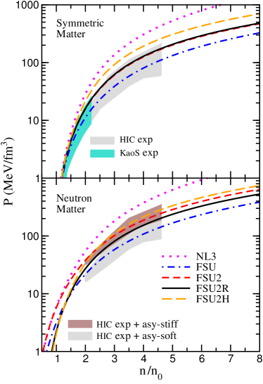
Figure 1: Pressure versus baryon density for SNM (upper panel) and PNM (lower panel) for the different models presented in the text: NL3 (Lalazissis et al., 1997), FSU (Todd-Rutel & Piekarewicz, 2005), FSU2 (Chen & Piekarewicz, 2014), FSU2R (this work) and FSU2H (this work, Sec. 4). The regions compatible with the experimental data on collective flow (Danielewicz et al., 2002) and on kaon production (Fuchs et al., 2001; Lynch et al., 2009) in HICs are depicted in gray and turquoise, respectively, in the upper panel. The shaded areas in the panel of PNM correspond to the constraints from the flow data supplemented by a soft (gray area) and a stiff (brown area) symmetry energy (Danielewicz et al., 2002).

Models	NL3	FSU	FSU2	FSU2R	FSU2H
$m_{\sigma}$ [MeV]	508.194	491.500	497.479	497.479	497.479
$m_{\omega}$ [MeV]	782.501	782.500	782.500	782.500	782.500
$m_{\rho}$ [MeV]	763.000	763.000	763.000	763.000	763.000
$g_{\sigma N}^{2}$	104.3871	112.1996	108.0943	107.5751	102.7200
$g_{\omega N}^{2}$	165.5854	204.5469	183.7893	182.3949	169.5315
$g_{\rho N}^{2}$	79.6000	138.4701	80.4656	247.3409	247.3409
$\kappa$	3.8599	1.4203	3.0029	3.0911	4.0014
$\lambda$	$-$0.015905	0.023762	$-$0.000533	$-$0.001680	$-$0.013298
$\zeta$	0.00	0.06	0.0256	0.024	0.008
$\Lambda_{\omega}$	0.00	0.03	0.000823	0.05	0.05
$n_{0}$ $[{\rm fm}^{-3}]$	0.1481	0.1484	0.1505	0.1505	0.1505
$E/A$ $[{\rm MeV}]$	$-$16.24	$-$16.30	$-$16.28	$-$16.28	$-$16.28
$K$ $[{\rm MeV}]$	271.5	230.0	238.0	238.0	238.0
$m_{N}^{*}/m_{N}$	0.595	0.610	0.593	0.593	0.593
$E_{\rm sym}(n_{0})$ [MeV]	37.3	32.6	37.6	30.2	30.2
$L$ [MeV]	118.2	60.5	112.8	44.3	41.0
$P(n_{0})$ $[{\rm MeV\,fm}^{-3}]$	5.99	3.18	5.81	2.27	2.06

Table 1: Parameters for the models NL3 (Lalazissis et al., 1997), FSU (Todd-Rutel & Piekarewicz, 2005), FSU2 (Chen & Piekarewicz, 2014), FSU2R (this work) and FSU2H (this work, Sec. 4). The mass of the nucleon is set to 939 MeV. Also shown are the corresponding energy per particle ($E/A$), compression modulus ($K$) and effective nucleon mass $m_{N}^{*}/m_{N}$ at saturation density $n_{0}$, as well as the symmetry energy ($E_{\rm sym}$), slope of the symmetry energy ($L$) and PNM pressure ($P$) at $n_{0}$.

We first consider the well-known parameter sets NL3 (Lalazissis et al., 1997) and FSU (also called FSUGold) (Todd-Rutel & Piekarewicz, 2005). NL3 has $\zeta=\Lambda_{\omega}=0$ while FSU has $\zeta=0.06$ and $\Lambda_{\omega}=0.03$ (the full set of parameters of the models can be found in Table 1). Both NL3 and FSU reproduce quite well a variety of properties of atomic nuclei. However, they render two EoSs in SNM with different behavior at supranormal densities due to the different $\zeta$ value (we recall that the $\Lambda_{\omega}$ coupling does not contribute in SNM). We can see in Fig. 1(upper panel) that above density $n\sim 1.5\!-\!2n_{0}$ the FSU model with $\zeta=0.06$ (dot-dashed blue line) yields a much softer SNM pressure than the NL3 model with $\zeta=0$ (dotted magenta line). In PNM, the isovector coupling $\Lambda_{\omega}$ tunes the change with density of the EoS, as it softens the symmetry energy. Indeed, if we compare the same models FSU and NL3 in PNM (see Fig. 1(lower panel)), FSU ($\Lambda_{\omega}=0.03$) has its pressure strongly further reduced with respect to NL3 ($\Lambda_{\omega}=0$) in the density window from around saturation density $n_{0}$ up to $n\sim 1.5\!-\!2n_{0}$. For densities above $2n_{0}$ the softening effect from $\Lambda_{\omega}$ is less prominent and the PNM pressures of FSU and NL3 show comparable differences with the case of SNM. We therefore note, consistently with the systematics in earlier works (Horowitz & Piekarewicz, 2001a, b; Carriere et al., 2003; Chen & Piekarewicz, 2014), that the $\Lambda_{\omega}$ and $\zeta$ couplings have a complementary impact on the EoS by each one influencing almost separate density sectors. This will be important for our goals for stellar radii and masses as we shall see below.

Next, we obtain the mass-radius (M-R) relation of neutron stars for a given EoS by solving the TOV equations (Oppenheimer & Volkoff, 1939). As mentioned in Sec. 2, for the crust region of the star we have employed the EoS recently derived in Ref. (Sharma et al., 2015). In this section we focus on neutron stars with cores of purely nucleonic matter; hence, we compute the EoS of the core assuming a $\beta$-equilibrated and charge neutral uniform liquid of neutrons, protons, and leptons (electrons and muons). As expected from its stiff EoS, the NL3 set predicts a large maximum mass ($M_{\rm max}\approx 2.8M_{\odot}$) and large stellar radii ($\approx\,$13 km for $M_{\rm max}$ and $\approx\,$15 km for a typical neutron star of $1.5M_{\odot}$), see the M-R relations plotted in Fig. 2 and the values in Table 2. In comparison, the soft EoS of the FSU model brings in a dramatic reduction of the stellar masses and radii. The two shaded bands in Fig. 1 portray the observed masses of the heaviest neutron stars known, i.e., $M=1.97\pm 0.04M_{\odot}$ in the pulsar PSR J1614–2230 (Demorest et al., 2010) and $M=2.01\pm 0.04M_{\odot}$ in the pulsar PSR J0348+0432 (Antoniadis et al., 2013). These two astrophysical measurements are arguably the most accurate constraints available so far to validate or defeat the model predictions for the high-density EoS.

Figure 2: Mass versus radius for neutron stars for the models NL3 (Lalazissis et al., 1997), FSU (Todd-Rutel & Piekarewicz, 2005), FSU2 (Chen & Piekarewicz, 2014) and FSU2R (this work). The two shaded bands portray the masses $M=1.97\pm 0.04M_{\odot}$ in the pulsar PSR J1614–2230 (gray band) (Demorest et al., 2010) and $M=2.01\pm 0.04M_{\odot}$ in the pulsar PSR J0348+0432 (turquoise band) (Antoniadis et al., 2013).

Composition	Models	$M_{\rm max}/M_{\odot}$	$R(M_{\rm max})$	$n_{c}(M_{\rm max})/n_{0}$	$R(1.5M_{\odot})$	$Y$ onset
			[km]		[km]	($n/n_{0}$)
	NL3	2.77	13.3	4.5	14.8
	FSU	1.72	10.8	7.8	12.2
$pne\mu$	FSU2	2.07	12.1	5.9	14.0
	FSU2R	2.05	11.6	6.3	12.8
	FSU2H	2.38	12.3	5.3	13.2
	NL3	2.27	12.9	5.3	14.8	1.9
$pnYe\mu$	FSU2	1.76	12.1	6.3	13.9	2.1
	FSU2R	1.77	11.6	6.5	12.8	2.4
	FSU2H	2.03	12.0	5.8	13.2	2.2
$pne\mu$	FSU2R	2.11	11.6	6.1	12.8
($B_{c}=2\times 10^{18}$ G)	FSU2H	2.42	12.3	5.2	13.2
$pnYe\mu$	FSU2R	1.88	11.6	6.3	12.8	2.4
($B_{c}=2\times 10^{18}$ G)	FSU2H	2.15	12.3	5.3	13.2	2.2

Table 2: Neutron star properties obtained for the different nuclear models discussed in this work. Results are shown for nucleonic-only ($pne\mu$) or hyperonic ($pnYe\mu$) stars, and including or not a magnetic field having the profile of the solid line in Fig. 6 (Sec. 4). The quantity $n_{c}(M_{\rm max})/n_{0}$ denotes the central baryonic density at the maximum mass, $M_{\rm max}$, normalized to the corresponding saturation density, $n_{0}$, whereas Y onset is the onset of appearance of hyperons normalized to $n_{0}$.

The recently formulated relativistic parameter set FSU2 (Chen & Piekarewicz, 2014)—based on the same Lagrangian we are discussing—is one of the first best-fit models to take into account the condition of a limiting stellar mass of $2M_{\odot}$ in the calibration of the parameters (also see (Erler et al., 2013) and (Chen & Piekarewicz, 2015b)). The FSU2 model has been optimized to accurately reproduce the experimental data on a pool of properties of finite nuclei with the maximum neutron star mass observable included in the fit (Chen & Piekarewicz, 2014). The resulting FSU2 set has $\zeta=0.0256$ and $\Lambda_{\omega}=0.0008$, cf. Table 1. In consonance with these values, we can appreciate in Fig. 1 that FSU2 predicts an intermediate EoS between the stiff EoS of the NL3 set ($\zeta=\Lambda_{\omega}=0$) and the soft EoS of the FSU set ($\zeta=0.06,\Lambda_{\omega}=0.03$). Accordingly, FSU2 produces a neutron star mass-radius relation located in between the curves of NL3 and FSU in Fig. 2. FSU2 yields a heaviest stellar mass $M_{\rm max}=2.07M_{\odot}$ with a radius of 12.1 km, and predicts $1.5M_{\odot}$ stars with a radius of 14 km, see Table 2.

While the limiting stellar mass is governed by the stiffness of the EoS above several times the saturation density $n_{0}$ (see column $n_{c}(M_{\rm max})/n_{0}$ in Table 2), the radius of a canonical neutron star is dominated by the density dependence of the EoS of PNM at 1–2 times $n_{0}$ (Lattimer & Prakash, 2007; Ozel & Freire, 2016). Thus, observational information on masses and radii of neutron stars has the potential to uniquely pin down the nuclear EoS in a vast density region. As mentioned in the Introduction, several of the recent astrophysical analyses for radii (Guillot et al., 2013; Guver & Ozel, 2013; Lattimer & Steiner, 2014; Heinke et al., 2014; Guillot & Rutledge, 2014; Ozel et al., 2016; Ozel & Freire, 2016) are converging in the 9–12 km range (also see Ref. (Fortin et al., 2015) for a detailed discussion). The review study of Ref. (Lattimer & Prakash, 2016) indicates a similar range around 11–13 km for the radii of canonical neutron stars. The possibility that neutron stars have these small radii is as exciting as it is deeply challenging for nuclear theory. Note that small radii demand a sufficiently soft EoS below twice the saturation density, while the observed large masses require that the same EoS must be able to evolve into a stiff EoS at high densities. It is therefore timely to explore whether such small radii can be obtained by the EoS of the covariant field-theoretical Lagrangian (1,2), while fulfilling at the same time the maximum mass constraint of $2M_{\odot}$ and the phenomenology of the atomic nucleus.

To construct the new EoS we start from the FSU2 model and increase the $\Lambda_{\omega}$ coupling. This softens the PNM pressure especially up to densities of $1.5\!-\!2n_{0}$. For a given stellar mass there is less pressure to balance gravity, thereby leading to a more compact object of smaller radius. The increase of $\Lambda_{\omega}$ also produces a certain reduction of the PNM pressure in the high-density sector. This may spoil the $2M_{\odot}$ maximum mass but can be counteracted by a decrease of the strength of the $\zeta$ coupling. During the change of the ($\Lambda_{\omega},\zeta$) couplings, we refit the remaining couplings $g_{\sigma N},g_{\omega N},g_{\rho N},\kappa$, and $\lambda$ of the nucleon-meson Lagrangian (1,2) by invoking the same saturation properties of FSU2 in SNM (i.e., same saturation density $n_{0}$, energy per particle $E/A$, compression modulus $K$, and effective nucleon mass $m_{N}^{*}$) and a symmetry energy $E_{\rm sym}=25.7$ MeV at subsaturation density $n=0.10$ fm^-3. The last condition arises from the fact that the binding energies of atomic nuclei constrain the symmetry energy at an average density of nuclei of $\sim\!0.10$ fm^-3 better than the symmetry energy at normal density $n_{0}$ (Horowitz & Piekarewicz, 2001a; Centelles et al., 2009). We found that under this protocol a noteworthy decrease of neutron star radii is achieved with $\Lambda_{\omega}=0.05$ and $\zeta=0.024$. We refer to the resulting model as FSU2R. The coupling constants and several bulk properties of FSU2R are collected in Table 1.

We observe in Fig. 1 that the EoS of the new FSU2R model is within the boundaries deduced in the studies of energetic HICs (Danielewicz et al., 2002; Fuchs et al., 2001; Lynch et al., 2009). It is worth noting that FSU2R features a soft PNM EoS at $n\lesssim 1.5\!-\!2n_{0}$ and a stiff PNM EoS at $n\gtrsim 2n_{0}$—apparently a necessary condition to satisfy small radii and heavy limiting neutron star masses. The reduction of the stellar radii in FSU2R compared with the other parametrizations of the Lagrangian (1,2) is very clear from Fig. 2, also see Table 2. The maximum mass of $2.05M_{\odot}$ calculated with FSU2R is compatible with the heaviest neutron stars (Demorest et al., 2010; Antoniadis et al., 2013) and is characterized by a radius of 11.6 km. For canonical neutron stars of 1.4–1.5 solar masses, FSU2R predicts radii of $\approx\!12.8$ km, which are more compact than in the other EoSs, cf. Table 2. Hence, the smaller radii reproduced by the new model point toward the reconciliation between the nuclear EoS, the largest neutron star masses (Demorest et al., 2010; Antoniadis et al., 2013), and the recent extractions of small neutron star sizes from the astrophysical observations of quiescent low-mass X-ray binaries (Guillot & Rutledge, 2014) and X-ray bursters (Guver & Ozel, 2013) (also see (Guillot et al., 2013; Lattimer & Steiner, 2014; Heinke et al., 2014; Ozel et al., 2016; Ozel & Freire, 2016; Lattimer & Prakash, 2016)). We are only aware of similar models RMF012 and RMF016 (also called FSUGarnet) introduced in a recent work (Chen & Piekarewicz, 2015b). The RMF012 and RMF016 models were fitted with the same procedure of the FSU2 model of (Chen & Piekarewicz, 2014) but requiring values for the neutron skin thickness of the ²⁰⁸Pb nucleus of, respectively, 0.12 fm and 0.16 fm. As reported in (Chen & Piekarewicz, 2015a, b), the RMF016 model supports $2M_{\odot}$ neutron stars and leads to a radius of 13 km for a $1.4M_{\odot}$ star, similarly to the predictions we obtain with our FSU2R model.

3.2 Implications for finite nuclei:
symmetry energy, slope of the symmetry energy
and neutron skin thickness

Once the new EoS has been calibrated for neutron stars, it is important to review its implications for the physics regime of atomic nuclei since this regime is accessible in laboratory experiments. We first verify that the new model FSU2R is able to provide a satisfactory description of the best known properties of nuclei, i.e., nuclear ground-state energies and sizes of the nuclear charge distributions. We display in Fig. 3 our results for the energies and charge radii of a set of representative nuclei ranging from the light ¹⁶O to the heavy ²⁰⁸Pb. The experimental data of these same nuclei were used in the fit of the FSU2 model in Ref. (Chen & Piekarewicz, 2014). In Fig. 3, we show the predictions of our FSU2R model alongside the experimental values and the results from the parameter sets NL3, FSU, and FSU2. It can be seen that the four models successfully reproduce the energies and charge radii across the mass table. The agreement of FSU2R with experiment is overall comparable to the other models. We find that the differences between FSU2R and the experimental energies and radii are at the level of 1% or smaller. We mention that we have not drawn error bars of the experimental data in Fig. 3, because the nuclear masses and charge radii are measured so precisely (Wang et al., 2012; Angeli & Marinova, 2013) that the experimental uncertainties cannot be resolved in the plot.

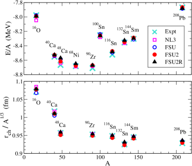
Figure 3: Energy per nucleon $E/A$ and charge radius $r_{\rm ch}$ over $A^{1/3}$, where $A$ is the mass number, of several nuclei with magic proton and/or neutron numbers. The values calculated with the models discussed in the text are compared with experiment. The experimental data are from Ref. (Wang et al., 2012) for the energies and from Ref. (Angeli & Marinova, 2013) for the charge radii.

For our purposes, of special relevance is the fact that the neutron density distributions and other isospin-sensitive observables of atomic nuclei are closely related to the density dependence of the symmetry energy, which in FSU2R has been tailored to supply small stellar radii. The stiffness of the symmetry energy with density is conventionally characterized by its density slope $L$ at the saturation point: $\displaystyle L=3n_{0}\Big{(}\frac{\partial E_{\rm sym}(n)}{\partial n}\Big{)}_{n_{0}}$. The $L$ parameter and the pressure $P(n_{0})$ of PNM at saturation density are related as $P(n_{0})=\frac{1}{3}n_{0}L$ (Lynch et al., 2009; Lattimer & Prakash, 2016). The new FSU2R EoS yields $E_{\rm sym}(n_{0})=30.2$ MeV for the symmetry energy at saturation and a slope parameter $L=44.3$ MeV, which corresponds to a mildly soft nuclear symmetry energy. The PNM pressure at saturation is $P(n_{0})=2.27$ MeV fm^-3. We have collected these values in Table 1 along with the results for $E_{\rm sym}(n_{0})$, $L$, and $P(n_{0})$ from the other discussed EoSs—now, large differences can be appreciated among the models.

Despite the fact that a precise knowledge of the density dependence of the symmetry energy remains elusive, the windows of values for $E_{\rm sym}(n_{0})$ and the slope parameter $L$ have been continuously narrowed down as the empirical and theoretical constraints have improved over recent years (see e.g. Ref. (Li et al., 2014) for a topical review). Remarkably, the values of 30.2 MeV for $E_{\rm sym}(n_{0})$ and 44.3 MeV for $L$ that we find after constraining the EoS to reflect small neutron star radii, turn out to be very much consistent with the newest determinations of the symmetry energy and its slope at saturation, see Fig. 4. Indeed, the quoted FSU2R values overlap with the ranges $30\lesssim E_{\rm sym}(n_{0})\lesssim 35$ MeV and $20\lesssim L\lesssim 66$ MeV extracted in Ref. (Roca-Maza et al., 2015) from the recent high-resolution measurements at RCNP and GSI of the electric dipole polarizability $\alpha_{D}$ in the nuclei ²⁰⁸Pb (Tamii et al., 2011), ¹²⁰Sn (Hashimoto et al., 2015), and ⁶⁸Ni (Rossi et al., 2013). We note that the dipole polarizability $\alpha_{D}$, related to the response of nuclei to an external electric field, has been identified as one of the strongest isovector indicators (Reinhard & Nazarewicz, 2010). Also note that, compared to hadronic experiments used to probe the symmetry energy, the electromagnetic reactions involved in the measurements of the $\alpha_{D}$ observable (Tamii et al., 2011; Hashimoto et al., 2015; Rossi et al., 2013) are particularly suited because they are not hindered by large or uncontrolled uncertainties. The FSU2R predictions for $E_{\rm sym}(n_{0})$ and $L$ also fit within the windows $29\lesssim E_{\rm sym}(n_{0})\lesssim 33$ MeV and $40\lesssim L\lesssim 62$ MeV obtained in Ref. (Lattimer & Lim, 2013) from the combined analysis of a variety of empirical nuclear constraints and astrophysical informations, which are in line with similar windows obtained in other recent studies (Li et al., 2014; Tsang et al., 2012; Lattimer & Prakash, 2016). It also deserves to be mentioned that the $E_{\rm sym}(n_{0})$ and $L$ values of the FSU2R EoS are quite compatible with the theoretical ranges $25.2\lesssim E_{\rm sym}(n_{0})\lesssim 30.4$ MeV and $37.8\lesssim L\lesssim 47.7$ MeV that have been derived from the latest progress in ab initio calculations of nuclear systems with chiral forces (Hagen et al., 2015).

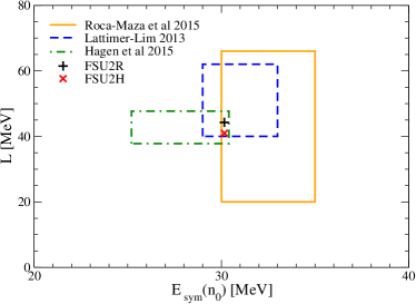
Figure 4: Slope of the symmetry energy ($L$) versus symmetry energy ($E_{\rm sym}(n_{0})$) at saturation for the models FSU2R discussed in this section and FSU2H discussed in Sec. 4. The rectangular areas are the determinations from Refs. (Lattimer & Lim, 2013; Hagen et al., 2015; Roca-Maza et al., 2015).

The neutron skin thickness $\Delta r_{np}=r_{n}-r_{p}$ (difference between the neutron and proton matter radii) of a heavy nucleus such as ²⁰⁸Pb, also provides strong sensitivity to the symmetry energy and the pressure of neutron-rich matter near saturation (Alex Brown, 2000; Horowitz & Piekarewicz, 2001a, b; Centelles et al., 2009). Basically the same nuclear pressure that is responsible for determining the radius of a canonical neutron star, determines how far neutrons extend out further than protons in a nucleus. By the same token, models that produce smaller stellar radii are expected to predict thinner neutron skins. We find that the FSU2R model, constrained to small neutron star radii, predicts $\Delta r_{np}=0.133$ fm in ²⁰⁸Pb. Unfortunately, neutron skins are difficult to extract from experiments in a model-independent fashion. The new experiments to measure neutron skins are being designed with electroweak and electromagnetic probes where, unlike hadronic experiments, the interactions with the nucleus (Abrahamyan et al., 2012), or at least the initial state interactions (Tarbert et al., 2014), are not complicated by the strong force. The challenging, purely electroweak (nearly model-independent) measurement of the neutron skin of ²⁰⁸Pb by parity violating electron scattering at JLab (Abrahamyan et al., 2012; Horowitz et al., 2012) has been able to provide $\Delta r_{np}=0.302\pm 0.177$ fm for this isotope (Horowitz et al., 2012), although the data is not conclusive due to the large error bars (a follow-up measurement at JLab with better statistics has been proposed). The recent measurement of the neutron skin of ²⁰⁸Pb at the MAMI facility from coherent pion production by photons (Tarbert et al., 2014) has obtained $\Delta r_{np}=0.15\pm 0.03$ fm. A similar range $0.13\lesssim\Delta r_{np}\lesssim 0.19$ fm for ²⁰⁸Pb is extracted (Roca-Maza et al., 2015) by comparing theory with the accurately measured electric dipole polarizability in ²⁰⁸Pb (Tamii et al., 2011), ¹²⁰Sn (Hashimoto et al., 2015), and ⁶⁸Ni (Rossi et al., 2013). Thus, the FSU2R prediction of a neutron skin of 0.133 fm in ²⁰⁸Pb turns out to be fairly compatible within error bars with the recent determinations of this isospin-sensitive observable.

In summary, when the nuclear EoS has been constrained to encode the recent astrophysical indications of small neutron star radii, yet without compromising massive stars, a high degree of consistency has emerged between the predictions of the model and the latest terrestrial informations on the symmetry energy, its density dependence, and neutron skins, as well as with the constraints inferred from state-of-the-art ab initio microscopic calculations (Hagen et al., 2015). All in all, we believe that the present findings make a compelling case in favor of the prospect that neutron stars may have small, or moderate-to-small, radii.

4 Hyperons and magnetic field

Having calibrated the nuclear model to produce small neutron star radii and fulfill maximum masses of  $2M_{\odot}$, while at the same time reproducing the phenomenology of atomic nuclei and the empirical constraints from collective flow and kaon production in HICs, we explore in this section the effect on the EoS and neutron stars of including hyperons and magnetic fields.

We should first determine the value of the hyperon couplings in our RMF model. Those couplings are calculated by fitting the experimental data available for hypernuclei, in particular, the value of the optical potential of hyperons extracted from these data. In our model, the contribution to the potential of a hyperon $i$ in $j$-particle matter is given by

$$U_{i}^{(j)}(n_{j}) = -g_{\sigma i}\,\bar{\sigma}^{(j)}+g_{\omega i}\,\bar{\omega}^{(j)}+g_{\rho i}\,I_{3i}\,\bar{\rho}^{(j)}+g_{\phi i}\,\bar{\phi}^{(j)},\ \ \ \ \ \$$ (34)

where $\bar{\sigma}^{(j)}$, $\bar{\omega}^{(j)}$, $\bar{\rho}^{(j)}$ and $\bar{\phi}^{(j)}$ are the values of the meson fields in the $j$-particle matter and $I_{3i}$ stands for the third component of the isospin operator.

The couplings of the hyperons to the vector mesons are related to the nucleon couplings, $g_{\omega N}$ and $g_{\rho N}$, by assuming SU(3)-flavor symmetry, the vector dominance model and ideal mixing for the physical $\omega$ and $\phi$ mesons, as e.g. employed in many recent works (Schaffner & Mishustin, 1996; Banik et al., 2014; Miyatsu et al., 2013; Weissenborn et al., 2012; Colucci & Sedrakian, 2013). This amounts to assuming the following relative coupling strengths:

$$g_{\omega\Lambda}:g_{\omega\Sigma}:g_{\omega\Xi}:g_{\omega N} = \frac{2}{3}:\frac{2}{3}:\frac{1}{3}:1$$

$$g_{\rho\Lambda}:g_{\rho\Sigma}:g_{\rho\Xi}:g_{\rho N} = 0:1:1:1$$

$$g_{\phi\Lambda}:g_{\phi\Sigma}:g_{\phi\Xi}:g_{\omega N} = -\frac{\sqrt{2}}{3}:-\frac{\sqrt{2}}{3}:-\frac{2\sqrt{2}}{3}:1,\ \$$ (35)

and $g_{\phi N}=0$. Note that the isospin operator $I_{3i}$ appearing in the definition of the potentials in Eq. (34) implements the relative factor of 2 missing in the 1:1 relation between $g_{\rho\Sigma}$ and $g_{\rho N}$ displayed in Eq. (35), so that the effective coupling of the $\rho$ meson to the $\Sigma$ hyperon ($I_{3}=-1,0,+1$) is twice that to the nucleon ($I_{3}=-1/2,+1/2$), as required by the symmetries assumed.

The coupling of each hyperon to the $\sigma$ field is adjusted to reproduce the hyperon potential in SNM derived from hypernuclear observables, see e.g. (Hashimoto & Tamura, 2006; Gal et al., 2016). The $\Lambda$ binding energy of $\Lambda$-hypernuclei is well reproduced by an attractive Woods-Saxon potential of depth $U_{\Lambda}^{(N)}(n_{0})\sim-28$ MeV (Millener et al., 1988). The analyses of the $(\pi^{-},K^{+})$ reaction data on medium to heavy nuclei (Noumi et al., 2002) performed in (Harada & Hirabayashi, 2006; Kohno et al., 2006) revealed a moderately repulsive $\Sigma$-nuclear potential in the nuclear interior of around $10-40$ MeV, while the fits to $\Sigma^{-}$ atomic data (Friedman & Gal, 2007) indicate a clear transition from an attractive $\Sigma$ potential in the surface, to a repulsive one in the interior, although the size of the repulsion cannot be precisely determined. As for the strangeness $-2$ systems, the Nagara event (Takahashi et al., 2001) and other experiments providing consistency checks established the size of the $\Lambda\Lambda$ interaction to be mildly attractive, $\Delta B_{\Lambda\Lambda}(^{6}_{\Lambda\Lambda}{\rm He})=0.67\pm 0.17$ MeV (Ahn et al., 2013), while the knowledge obtained for the $\Xi N$ interaction is more uncertain. Analyses of old emulsion data indicate a sizable attractive $\Xi$-nucleus potential of $U_{\Xi}^{(N)}(n_{0})=-24\pm 4$ MeV (Dover & Gal, 1983), while the missing-mass spectra of the $(K^{-},K^{+})$ reaction on a ¹²C target suggest a milder attraction of $\gtrsim-20$ MeV (Fukuda et al., 1998) or $\sim-14\pm 2$ MeV (Khaustov et al., 2000). These values are compatible with the recent analysis of the nuclear emulsion event KISO, claiming to have observed a nuclear bound state of the $\Xi^{-}$-¹⁴N system with a binding energy of $4.38\pm 0.25$ MeV (Nakazawa et al., 2015). From the above considerations, we fix the hyperon potentials in SNM to the following values:

$$U_{\Lambda}^{(N)}(n_{0}) = -28~{}{\rm MeV}$$

$$U_{\Sigma}^{(N)}(n_{0}) = +30~{}{\rm MeV}$$

$$U_{\Xi}^{(N)}(n_{0}) = -18~{}{\rm MeV}\ ,$$ (36)

which allow us to determine the couplings $g_{\sigma\Lambda}$, $g_{\sigma\Sigma}$ and $g_{\sigma\Xi}$, from Eq. (34). We finally note that the coupling of the $\phi$ meson to the $\Lambda$ baryon is reduced by 20% with respect to its SU(3) value in order to obtain a $\Lambda\Lambda$ bond energy in $\Lambda$ matter at a density $n_{\Lambda}\simeq n_{0}/5$ of $\Delta B_{\Lambda\Lambda}(n_{0}/5)=0.67$ MeV, thereby reproducing the Nagara event (Ahn et al., 2013).

Let us comment on the fact that the presence of hyperons in the neutron star interior and their influence on the EoS suffer from uncertainties tied to our lack of knowledge of the hyperon-nucleon and hyperon-hyperon interactions around the hyperon onset density of $\sim 2n_{0}$ and beyond. This freedom has been exploited by different groups to build up RMF models that ensure the existence of neutron stars with masses larger than $2M_{\odot}$ even with the presence of hyperons (see for example (Weissenborn et al., 2012; Bednarek et al., 2012; van Dalen et al., 2014; Oertel et al., 2015)). While the radii of neutron stars are essentially determined by the nucleonic part of the EoS, the uncertainties in the hyperon interactions reflect on maximum masses that are scattered within a 0.3 $M_{\odot}$ band, as can be seen from the thorough analysis of various models done by (Fortin et al., 2015), which is consistent with admitting a deviation by at most 30% of the symmetries assumed to determine the hyperon coupling constants (Weissenborn et al., 2012). These results provide an estimate of the uncertainties that one must admit in the hyperonic sector until data on the hyperon interactions at higher densities, coming for instance from HIC experiments (Morita et al., 2015), become available. As explained in the preceding paragraph, in this work we have simply made a minimal adjustment of the hyperon parameters away from the symmetry constraints imposed by Eq. (35) in order to reproduce the known hypernuclear properties.

In Fig. 5 we show how the presence of hyperons affects the M-R relationship for some representative nuclear EoSs selected from the previous section: the highly stiff EoS of the NL3 model and the FSU2 and FSU2R EoSs. These models differ essentially on the lower density ($n\lesssim 2n_{0}$) and/or the higher density ($n\gtrsim 2n_{0}$) stiffness of the EoS. As already noted in Refs. (Horowitz & Piekarewicz, 2001b; Chen & Piekarewicz, 2014, 2015a) and also discussed in the previous section, models with a larger value of the $\Lambda_{\omega}$ coupling produce a softer symmetry energy and, in consequence, become more compressible leading to stars with higher central densities and smaller radii. The presence of hyperons softens the EoS by essentially releasing Fermi pressure. Thereby, the stars get further compressed than their nucleonic counterparts, and the maximum masses get reduced by about 15%, as seen by the thick lines in Fig. 5. It is also seen from this figure that the occurrence of hyperons leaves the stellar radii almost unaffected.

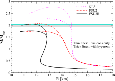
Figure 5: Mass versus radius for neutron stars for the models NL3 (Lalazissis et al., 1997), FSU2 (Chen & Piekarewicz, 2014) and FSU2R (this work) with hyperons (thick lines) and without hyperons (thin lines). The two shaded bands portray the masses $M=1.97\pm 0.04M_{\odot}$ in the pulsar PSR J1614–2230 (gray band) (Demorest et al., 2010) and $M=2.01\pm 0.04M_{\odot}$ in the pulsar PSR J0348+0432 (turquoise band) (Antoniadis et al., 2013).

Except for the NL3 model, which has shown to be exceedingly stiff at supranormal densities, the maximum masses of hyperonic stars attained by the other two models are too low, of about $M_{\rm max}=1.8M_{\odot}$, to reproduce the 2$M_{\odot}$ limit. The specific values of the maximum masses of hyperonic stars for all these models can be seen in Table 2 in the ’$pneY\mu$’ section. We observe a weak sensitivity to the slope of the symmetry energy, as FSU2 and FSU2R produce essentially the same maximum masses. This was already noted in the context of nucleonic-only EoSs in Ref. (Horowitz & Piekarewicz, 2001b). As the symmetry energy softens, the star simply becomes more compressed and attains a larger central density, but reaches a similar maximum mass value. This phenomenology remains when hyperons are present, as was also found in (Providencia & Rabhi, 2013), the only difference being that the hyperonic stars attain a lower maximum mass and have a higher central density than their nucleonic-only counterparts, as expected for a softer EoS. This can be seen upon comparing the values shown in the ’$pne\mu$’ and ’$pneY\mu$’ sections of Table 2.

Since the hyperonic EoS based on the FSU2R model does not produce $M_{\rm max}>2M_{\odot}$, we tense the parameters of this nuclear model a little further so as to make it stiffer. We essentially reduce the value of $\zeta$ from 0.024 to 0.008, which stiffens the EoS at densities larger than twice the saturation density, i.e. around the region where hyperons start appearing (see the hyperon onset density for the different models in Table 2). The remaining parameters of the model are refitted so as to reproduce the SNM saturation properties of the FSU2 model and a symmetry energy $E_{\rm sym}=26.2$ MeV at density $n=0.10$ fm^-3. The values of the parameters of this new interaction, named FSU2H, are listed in Table 1, together with the predicted $E_{\rm sym}$ value at saturation density and its slope $L$, which fall comfortably within the newest empirical and theoretical constraints of these quantities, as can be seen in Fig 4. The couplings of the hyperons to the different vector mesons can be readily obtained from Eq. (35), and those to the $\sigma$ meson, determined from fixing the hyperon potentials in SNM, are $g_{\sigma\Lambda}=0.6113$, $g_{\sigma\Sigma}=0.4665$ and $g_{\sigma\Xi}=0.3157$.

We note that the FSU2H interaction produces a certain overpressure in SNM at $n\gtrsim 2n_{0}$, since the pressure falls above the allowed region obtained from the modeling of collective flow in HICs, as seen by the long dashed line in the upper part of Fig. 1. Nevertheless, the EoS for PNM, seen in the lower panel of this figure, falls within the PNM extrapolated band compatible with collective flow. Since neutron-star matter in beta equilibrium is highly asymmetric we consider this model to be sufficiently realistic to describe neutron stars, whose properties are presented in Table 2. We observe that the maximum mass of $2.38M_{\odot}$ obtained for a ’$pne\mu$’ neutron star with the FSU2H model gets reduced to $2.03M_{\odot}$, with a radius of 12 km, when hyperons are present. We also observe that the radius of a canonical star of $\sim 1.5M_{\odot}$ gets slightly enhanced from 12.8 km for FSU2R to 13.2 km for FSU2H, which is the price one pays for having stiffened the EoS.

On comparing the ’$pne\mu$’ with the ’$pneY\mu$’ parts of Table 2 we essentially see, as in Fig. 5, a reduction of about 15% on the maximum mass when hyperons are allowed to appear in the neutron star cores. Since the hyperonic EoSs become more compressible, the ’$pnYe\mu$’ stars attain higher central densities, but the radii of the maximum-mass stars stay rather similar to their nucleonic-only counterparts.

We would like to note that the FSU2H parameterization, which produces $M_{\rm max}>2M_{\odot}$ even in the presence of hyperons, fulfills the pressure constraint in neutron star matter at saturation density $n_{0}$:

$$1.7\mbox{ MeV fm}^{-3}<P(n_{0})<2.8\mbox{ MeV fm}^{-3}\ ,$$ (37)

estimated in (Fortin et al., 2015) from the results shown in (Hebeler et al., 2013), which were obtained from microscopic calculations of PNM based on chiral two-nucleon and three-nucleon interactions, and which are in remarkable agreement with the Quantum Monte Carlo results of Ref. (Gandolfi et al., 2012), obtained from the phenomenological Argonne v18 NN potential plus three-nucleon forces. It is argued in (Fortin et al., 2015) that nearly all hyperonic EoS models that are able to sustain $M_{\rm max}>2M_{\odot}$ produce large PNM pressures of about 5 MeV fm^-3 at saturation density, leading to an overpressure of the nucleonic (pre-hyperon) segment and resulting in large radii of around 14 km or more for neutron stars in the range $1<M/M_{\odot}<1.6$. Our FSU2H model does not encounter this problem, since it gives a PNM pressure of $\sim 2$ MeV fm^-3 at $n_{0}$ (see Table 1), well within the constraint of Eq. (37), and as a consequence is able to reach a smaller radius of 13 km. We note that the symmetry energy slope parameter $L$ of the hyperonic models analyzed in (Fortin et al., 2015) lies in the range of values $67-118$ MeV, which deviate considerably from the recent constraints displayed in Fig 4.

We now discuss the effect of including a magnetic field in our nucleonic and hyperonic stars. We consider a density-dependent magnetic field with a profile of the type

$$B(n)=B_{s}+B_{c}\left\{1-{\rm exp}\left[-\beta\left(n/n_{0}\right)^{\gamma}\right]\right\}\ ,$$ (38)

introduced in (Chakrabarty et al., 1997) and employed in several other works (Rabhi & Providencia, 2010; Sinha et al., 2013; Lopes & Menezes, 2012). We take a surface magnetic field value of $B_{s}=10^{15}$ G, consistent with the surface magnetic fields of observed magnetars (Vasisht & Gotthelf, 1997; Kouveliotou et al., 1998; Woods et al., 1999) and a core magnetic field value of $B_{c}=2\times 10^{18}$ G, which is sufficiently strong to produce distinguishable effects on the properties of neutron stars. The parameters $\beta$ and $\gamma$ control the density where the magnetic field saturates and the steepness of the transition from the surface to the core field, respectively. We take $\beta=0.0065$ and $\gamma=3.5$ which ensure that the magnetic field has practically saturated to its maximum value at around $5-6n_{0}$, a range that covers the typical central densities of the maximum mass neutron stars explored in this work. Moreover, the indicated $\beta$ and $\gamma$ values produce moderate field values below saturation density, as can be seen by the solid line in Fig. 6. We note that this field profile does not incur on instabilities of the parallel component of the pressure $P_{||}$ associated to rapidly rising magnetic field toward relatively strong central values (Sinha et al., 2013).

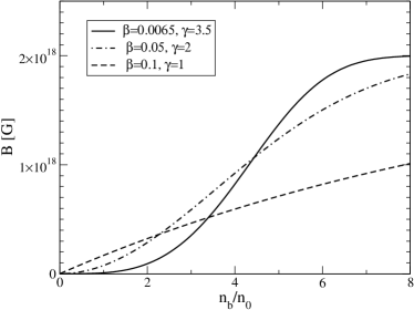
Figure 6: Magnetic field versus baryonic density for a function of the type of Eq. (38), taking $B_{s}=10^{15}$ G and $B_{c}=2\times 10^{18}$ G, for $(\beta,\gamma)=(0.0065,3.5)$ (solid line), $(\beta,\gamma)=(0.05,2)$ (dashed-dotted line) and $(\beta,\gamma)=(0.1,1)$ (dashed line).

The effect of this magnetic field on the M-R relationship is displayed in Fig. 7. On the left (right) panel we show the results obtained for the EoS employing the FSU2R (FSU2H) model. The solid lines correspond to vanishing magnetic field, while the dashed lines include the effects of the magnetic field with the density profile discussed above. The thin black lines show the results for nucleonic neutron stars and the thick red lines correspond to the hyperonic stars. As observed in earlier works (Lopes & Menezes, 2012), including the magnetic field produces stars with larger maximum masses. This is essentially a consequence of the increase in the total pressure which, apart from the matter pressure $P_{\rm matt}$, also includes the extra average field pressure component, as seen in Eq. (31). The size of this enhancement is larger for the hyperonic than for the nucleonic stars, which is essentially due, as we will show below, to the additional effect of de-hyperonization that takes place in the presence of a magnetic field. The reduction of hyperons is responsible for enhancing the value of the matter pressure $P_{\rm matt}$, since the Fermi contributions of the other species are larger than in the $B=0$ case. Nevertheless, the increase in the maximum mass induced by magnetic field effects is not enough to produce hyperonic star masses of the order of 2$M_{\odot}$ in the case of the FSU2R model, as the dashed red line on the left panel does not reach the observational bands. The effects of the magnetic field on the mass-radius relationships obtained with the FSU2H EoS (right panel) are similar to those for the FSU2R EoS, the only difference being that the constraint $M_{\rm max}>2M_{\odot}$ is now amply fulfilled, since the FSU2H model served this purpose even in the absence of a magnetic field.

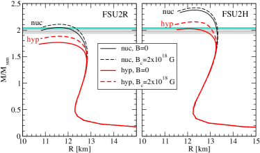
Figure 7: Mass versus radius of neutron stars for FSU2R (left panel) and FSU2H (right panel) models, with (thick lines) or without (thin lines) hyperons, and without (solid lines) or with (dashed lines) a magnetic field with the profile of Fig. 6, for $\beta=0.0065$ and $\gamma=3.5$ The two shaded bands portray the masses $M=1.97\pm 0.04M_{\odot}$ in the pulsar PSR J1614–2230 (gray band) (Demorest et al., 2010) and $M=2.01\pm 0.04M_{\odot}$ in the pulsar PSR J0348+0432 (turquoise band) (Antoniadis et al., 2013).

We now explore the effect of employing different magnetic field profiles having the same surface and central values, $B_{s}=10^{15}$ G and $B_{c}=2\times 10^{18}$ G, but different $\beta$ and $\gamma$ parameters. To this end, we consider, in addition to the profile obtained with the parameters $(\beta,\gamma)=(0.0065,3.5)$ chosen in this work, the profiles with $(\beta,\gamma)=(0.05,2)$ (Rabhi & Providencia, 2010) and $(\beta,\gamma)=(0.1,1)$ (Sinha et al., 2013), which are represented, respectively, by the dashed-dotted and dashed lines in Fig. 6. We observe that our parameterization produces a substantially lower magnetic field in the $n<2n_{0}$ region and reaches 90% of the saturation value around 5$n_{0}$, while the dashed-dotted parametrization does it right after $6n_{0}$. The parameterization of the dashed line does not even reach the value $B=10^{18}$ G within the densities of interest ($n\lesssim 6n_{0}$).

In Fig. 8 we display the M-R relationships obtained with these profiles, together with the zero magnetic field case, represented by a thin solid line. A noticeable dependence of the M-R relationship on the magnetic field profile is observed. The results for the $(\beta,\gamma)=(0.05,2)$ case (thick dashed-dotted line) are similar to those obtained with our $(\beta,\gamma)=(0.0065,3.5)$ parameterization (thick solid line), but the stars are produced with a somewhat larger radius since the magnetic field and, hence, the total pressure are larger in the pre-hyperon region. This is even more evident for the M-R relationship obtained with the $(\beta,\gamma)=(0.1,1)$ profile (thick dashed line), which produces stars that are $\sim 0.5$ km wider than the other two cases and deviates from the 13 km maximum radius constraint. The reason is that this profile clearly gives larger magnetic fields in the $n\lesssim n_{0}$ region, hence producing a larger total pressure and making the star less compressible.

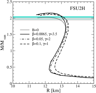
Figure 8: Mass versus radius of hyperonic neutron stars obtained with the FSU2H model and including a magnetic field with the different profiles displayed in Fig. 6. The field-free case is shown by the thin solid line. The two shaded bands portray the masses $M=1.97\pm 0.04M_{\odot}$ in the pulsar PSR J1614–2230 (gray band) (Demorest et al., 2010) and $M=2.01\pm 0.04M_{\odot}$ in the pulsar PSR J0348+0432 (turquoise band) (Antoniadis et al., 2013).

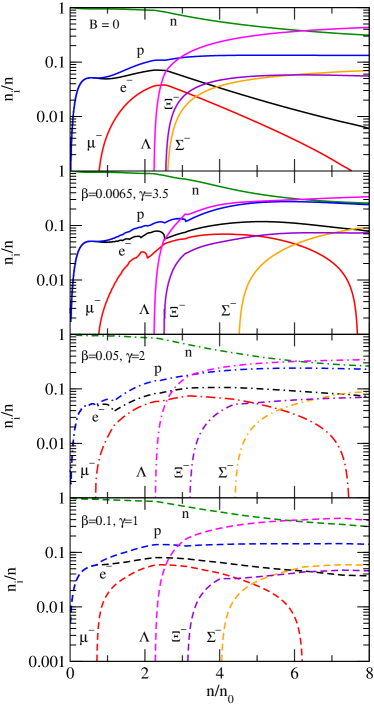
Figure 9: Particle fractions as functions of the baryonic density for the FSU2H model without magnetic field (first panel) and including the magnetic field profile of Eq. (38), taking $B_{s}=10^{15}$ G and $B_{c}=2\times 10^{18}$ G and for $(\beta,\gamma)=(0.0065,3.5)$ (second panel) , $(\beta,\gamma)=(0.05,2)$ (third panel) and $(\beta,\gamma)=(0.1,1)$ (fourth panel).

The particle fractions for beta-stable neutron star matter obtained using the FSU2H EoS are shown in Fig. 9 as functions of the baryonic density. The upper panel displays the fractions in the absence of magnetic field, while the other panels implement the magnetic field with the three different profiles shown in Fig. 6. Landau oscillations are seen in the charged particle fractions when a magnetic field is applied, reflecting the successive filling of the Landau levels as the quantity $(E_{F}^{2}-{m^{*}}^{2})/2|q|B$ reaches integer values. For a fixed density, smaller magnetic fields accommodate more Landau levels and, correspondingly, more oscillations are observed, as seen for instance when comparing the three $B\neq 0$ panels in the $n<2n_{0}$ density region, where the smallest field corresponds to the $(\beta,\gamma)=(0.0065,3.5)$ case. As density increases, so does the magnetic field in all the considered profiles, eventually needing only one Landau level to accommodate the population of the charged particles. The oscillations then tend to smooth out and disappear with increasing density. As is evident, the magnetic field mostly affects the charged particles, which in general increase their population with respect the $B=0$ case. At low and intermediate densities up to $n\sim 4n_{0}$, we clearly observe an increase in the occupation of negatively charged electrons and muons. This delays the appearance of the negatively charged hyperons, an effect that is especially visible for the $\Sigma^{-}$ baryon, whose onset moves to $n\gtrsim 4n_{0}$ for all the considered magnetic field profiles.

According to the results shown in the second panel of Fig. 9, in the case of a magnetized hyperonic star having a mass of about $2M_{\odot}$ with a maximum density of about $5n_{0}$ (see Table 2), the baryon fractions at the center would be 38% for n, 28% for $\Lambda$, 26% for p, 6% for $\Xi^{-}$ and 2% for $\Sigma^{-}$. In the $B=0$ case (upper panel), these fractions would be 45% for n, 31% for $\Lambda$, 13% for p, 6% for $\Xi^{-}$ and 5% for $\Sigma^{-}$. We then see that the proton abundance can be twice as large in a magnetar as it is in a field-free star. Our results are qualitatively consistent with those obtained by other works in the literature studying the effect of magnetic fields in hyperonic stars (Broderick et al., 2002; Rabhi & Providencia, 2010; Sinha et al., 2013; Lopes & Menezes, 2012; Yue et al., 2009). We can conclude that, in general, hyperonic magnetars re-leptonize and de-hyperonize with respect to zero-field stars, while the proton abundance increases substantially. This might facilitate direct Urca processes, drastically altering the cooling evolution of the star.

5 Summary

We have obtained a new EoS for the nucleonic inner core of neutron stars that fullfills the constraints coming from recent astrophysical observations of maximum masses and determinations of radii, as well as the requirements from experimental nuclear data known from terrestrial laboratories. This EoS results from a new parameterization of the FSU2 force (Chen & Piekarewicz, 2014), the so-called FSU2R model, that reproduces: i) the 2$M_{\odot}$ observations (Demorest et al., 2010; Antoniadis et al., 2013), ii) the recent determinations of radii below 13 km region (Guillot et al., 2013; Lattimer & Steiner, 2014; Heinke et al., 2014; Guillot & Rutledge, 2014; Ozel et al., 2016; Lattimer & Prakash, 2016), iii) the saturation properties of nuclear matter and finite nuclei (Tsang et al., 2012; Chen & Piekarewicz, 2014) and iv) the constraints extracted from nuclear collective flow (Danielewicz et al., 2002) and kaon production (Fuchs et al., 2001; Lynch et al., 2009) in HICs.

The FSU2R model is obtained by modifying the $\Lambda_{\omega}$ and $\zeta$ couplings of the Lagrangian simultaneously, while recalculating the couplings $g_{\sigma N},g_{\omega N},g_{\rho N},\kappa$, and $\lambda$ to grant the same saturation properties of FSU2 in SNM and a symmetry energy of 25.7 MeV at $n=0.10$ fm^-3. On the one hand, radii of 12-13 km are obtained, owing to the fact that we softened the symmetry energy and, consequently, the pressure of PNM at densities $\sim 1.5$-$2n_{0}$, while reproducing the properties of nuclear matter and nuclei. Indeed, we obtain $E_{\rm sym}=30$ MeV and $L=44$ MeV, which lie within the limits of the recent determinations of Refs. (Roca-Maza et al., 2015; Lattimer & Lim, 2013; Hagen et al., 2015). Moreover, the FSU2R model predicts a neutron skin thickness of 0.133 fm for the ²⁰⁸Pb nucleus, which is compatible with the recent experimental results (Abrahamyan et al., 2012; Horowitz et al., 2012; Tarbert et al., 2014; Roca-Maza et al., 2015). On the other hand, we have stiffened the EoS above twice the saturation density, which satisfies the constraints of HICs (Danielewicz et al., 2002; Fuchs et al., 2001; Lynch et al., 2009) and allows for maximum masses of 2$M_{\odot}$ (Demorest et al., 2010; Antoniadis et al., 2013). All in all, the FSU2R parameterization allows for a compromise between small stellar sizes and large masses, a task that seemed difficult to achieve in up-to-date RMF models.

We also analyze the consequences of the appearance of hyperons inside the core of neutron stars. The values of the hyperon couplings are determined from the available experimental information on hypernuclei, in particular by fitting to the optical potential of hyperons extracted from the data. On the one hand, we find that the radii of the neutron stars are rather insensitive to the appearance of the hyperons and, thus, still respect the observations of radii $<$ 13 km. On the other hand, we obtain a reduction of the maximum mass below 2$M_{\odot}$ once hyperons appear due to the expected softening of the EoS. However, by refitting the parameters of the FSU2R model slightly, the new parameterization FSU2H fulfills the 2$M_{\odot}$ limit while still reproducing the properties of nuclear matter and nuclei. The price to pay is a stiffer EoS in SNM as compared to the constraint derived from the modeling of HICs. Nonetheless, the HICs estimate in PNM is still satisfied by the FSU2H parametrization (Danielewicz et al., 2002).

We finally study the effect of high magnetic fields on the nucleonic and hyperonic EoSs. This is of particular interest for understanding the behavior of highly magnetized neutron stars, the so-called magnetars. Employing magnetic fields with crustal and interior values of $\sim 10^{15}$ G and $\sim 10^{18}$ G, respectively, we find EoSs that are stiffer and produce larger maximum-mass stars, while keeping radii in the 12-13 km range, both for nucleonic and hyperonic magnetars, as long as the magnetic field does not reach values larger than about $10^{17}$ G at saturation density. The particle fractions in the interior of the stars depend on the specific profile of the magnetic field, but the general trend with respect to zero-field stars is that hyperonic magnetars re-leptonize and de-hyperonize, while the amount of protons may double, a fact that may trigger direct Urca processes affecting the cooling and other transport properties of the star.

References

- Abrahamyan et al. (2012) Abrahamyan et al., S. 2012, Phys. Rev. Lett., 108, 112502
- Ahn et al. (2013) Ahn, J. K., et al. 2013, Phys. Rev., C88, 014003
- Alex Brown (2000) Alex Brown, B. 2000, Phys. Rev. Lett., 85, 5296
- Alford et al. (2007) Alford, M., Blaschke, D., Drago, A., et al. 2007, Nature, 445, E7
- Ambartsumyan & Saakyan (1960) Ambartsumyan, V. A., & Saakyan, G. S. 1960, Sov. Astron., 4, 187
- Angeli & Marinova (2013) Angeli, I., & Marinova, K. 2013, Atomic Data and Nuclear Data Tables, 99, 69
- Antoniadis et al. (2013) Antoniadis, J., et al. 2013, Science, 340, 6131
- Ardeljan et al. (2005) Ardeljan, N. V., Bisnovatyi-Kogan, G. S., & Moiseenko, S. G. 2005, Mon. Not. Roy. Astron. Soc., 359, 333
- Arzoumanian et al. (2014) Arzoumanian, Z., Gendreau, K. C., Baker, C. L., et al. 2014, in Proc. SPIE, Vol. 9144, Space Telescopes and Instrumentation 2014: Ultraviolet to Gamma Ray, 914420
- Bandyopadhyay et al. (1998) Bandyopadhyay, D., Chakrabarty, S., Dey, P., & Pal, S. 1998, Phys. Rev., D58, 121301
- Banik et al. (2014) Banik, S., Hempel, M., & Bandyopadhyay, D. 2014, Astrophys. J. Suppl., 214, 22
- Bauswein & Janka (2012) Bauswein, A., & Janka, H. T. 2012, Phys. Rev. Lett., 108, 011101
- Baym et al. (1971) Baym, G., Pethick, C., & Sutherland, P. 1971, Astrophys. J., 170, 299
- Bednarek et al. (2012) Bednarek, I., Haensel, P., Zdunik, J. L., Bejger, M., & Manka, R. 2012, Astron. Astrophys., 543, A157
- Bogdanov (2013) Bogdanov, S. 2013, Astrophys. J., 762, 96
- Boguta & Bodmer (1977) Boguta, J., & Bodmer, A. R. 1977, Nucl. Phys., A292, 413
- Boguta & Stoecker (1983) Boguta, J., & Stoecker, H. 1983, Phys. Lett., B120, 289
- Broderick et al. (2000) Broderick, A., Prakash, M., & Lattimer, J. M. 2000, Astrophys. J., 537, 351
- Broderick et al. (2002) Broderick, A. E., Prakash, M., & Lattimer, J. M. 2002, Phys. Lett., B531, 167
- Carriere et al. (2003) Carriere, J., Horowitz, C. J., & Piekarewicz, J. 2003, Astrophys. J., 593, 463
- Centelles et al. (2009) Centelles, M., Roca-Maza, X., Viñas, X., & Warda, M. 2009, Phys. Rev. Lett., 102, 122502
- Chakrabarty et al. (1997) Chakrabarty, S., Bandyopadhyay, D., & Pal, S. 1997, Phys. Rev. Lett., 78, 2898
- Chandrasekhar & Fermi (1953) Chandrasekhar, S., & Fermi, E. 1953, Astrophys. J., 118, 116, [Erratum: Astrophys. J.122,208(1955)]
- Chatterjee & Vidana (2016) Chatterjee, D., & Vidana, I. 2016, Eur. Phys. J., A52, 29
- Chen et al. (2007) Chen, W., Zhang, P.-Q., & Liu, L.-G. 2007, Mod. Phys. Lett., A22, 623
- Chen & Piekarewicz (2014) Chen, W.-C., & Piekarewicz, J. 2014, Phys. Rev., C90, 044305
- Chen & Piekarewicz (2015a) —. 2015a, Phys. Rev. Lett., 115, 161101
- Chen & Piekarewicz (2015b) —. 2015b, Phys. Lett., B748, 284
- Colucci & Sedrakian (2013) Colucci, G., & Sedrakian, A. 2013, Phys. Rev., C87, 055806
- Danielewicz et al. (2002) Danielewicz, P., Lacey, R., & Lynch, W. G. 2002, Science, 298, 1592
- Demorest et al. (2010) Demorest, P., Pennucci, T., Ransom, S., Roberts, M., & Hessels, J. 2010, Nature, 467, 1081
- Dexheimer et al. (2012) Dexheimer, V., Negreiros, R., & Schramm, S. 2012, Eur. Phys. J., A48, 189
- Dexheimer et al. (2015) —. 2015, Phys. Rev., C92, 012801
- Dover & Gal (1983) Dover, C. B., & Gal, A. 1983, Annals Phys., 146, 309
- Drago et al. (2014) Drago, A., Lavagno, A., Pagliara, G., & Pigato, D. 2014, Phys. Rev., C90, 065809
- Erler et al. (2013) Erler, J., Horowitz, C. J., Nazarewicz, W., Rafalski, M., & Reinhard, P. G. 2013, Phys. Rev., C87, 044320
- Fortin et al. (2015) Fortin, M., Zdunik, J. L., Haensel, P., & Bejger, M. 2015, Astron. Astrophys., 576, A68
- Friedman & Gal (2007) Friedman, E., & Gal, A. 2007, Phys. Rept., 452, 89
- Fuchs et al. (2001) Fuchs, C., Faessler, A., Zabrodin, E., & Zheng, Y.-M. 2001, Phys. Rev. Lett., 86, 1974
- Fukuda et al. (1998) Fukuda, T., et al. 1998, Phys. Rev., C58, 1306
- Gal et al. (2016) Gal, A., Hungerford, E. V., & Millener, D. J. 2016, Rev. Mod. Phys., 88, 035004
- Gandolfi et al. (2012) Gandolfi, S., Carlson, J., & Reddy, S. 2012, Phys. Rev., C85, 032801
- Glendenning (1982) Glendenning, N. K. 1982, Phys. Lett., B114, 392
- Glendenning (2000) —. 2000, Compact stars: Nuclear physics, particle physics, and general relativity, 2nd edn. (New York: Springer)
- Gomes et al. (2014) Gomes, R. O., Dexheimer, V., & Vasconcellos, C. A. Z. 2014, Astron. Nachr., 335, 666
- Guillot & Rutledge (2014) Guillot, S., & Rutledge, R. E. 2014, Astrophys. J., 796, L3
- Guillot et al. (2013) Guillot, S., Servillat, M., Webb, N. A., & Rutledge, R. E. 2013, Astrophys. J., 772, 7
- Guver & Ozel (2013) Guver, T., & Ozel, F. 2013, Astrophys. J., 765, L1
- Hagen et al. (2015) Hagen, G., et al. 2015, Nature Phys., 12, 186
- Harada & Hirabayashi (2006) Harada, T., & Hirabayashi, Y. 2006, Nucl. Phys., A767, 206
- Harding & Lai (2006) Harding, A. K., & Lai, D. 2006, Rept. Prog. Phys., 69, 2631
- Hashimoto & Tamura (2006) Hashimoto, O., & Tamura, H. 2006, Prog. Part. Nucl. Phys., 57, 564
- Hashimoto et al. (2015) Hashimoto, T., Krumbholz, A. M., Reinhard, P.-G., et al. 2015, Phys. Rev. C, 92, 031305
- Hebeler et al. (2013) Hebeler, K., Lattimer, J. M., Pethick, C. J., & Schwenk, A. 2013, Astrophys. J., 773, 11
- Heinke et al. (2014) Heinke, C. O., et al. 2014, Mon. Not. Roy. Astron. Soc., 444, 443
- Horowitz & Piekarewicz (2001a) Horowitz, C. J., & Piekarewicz, J. 2001a, Phys. Rev. Lett., 86, 5647
- Horowitz & Piekarewicz (2001b) —. 2001b, Phys. Rev., C64, 062802
- Horowitz et al. (2012) Horowitz, C. J., et al. 2012, Phys. Rev., C85, 032501
- Hulse & Taylor (1975) Hulse, R. A., & Taylor, J. H. 1975, Astrophys. J., 195, L51
- Jiang et al. (2015) Jiang, W.-Z., Li, B.-A., & Fattoyev, F. J. 2015, Eur. Phys. J., A51, 119
- Khaustov et al. (2000) Khaustov, P., et al. 2000, Phys. Rev., C61, 054603
- Klahn et al. (2013) Klahn, T., Aastowiecki, R., & Blaschke, D. B. 2013, Phys. Rev., D88, 085001
- Kohno et al. (2006) Kohno, M., Fujiwara, Y., Watanabe, Y., Ogata, K., & Kawai, M. 2006, Phys. Rev., C74, 064613
- Kouveliotou et al. (1998) Kouveliotou, C., et al. 1998, Nature, 393, 235
- Lackey & Wade (2015) Lackey, B. D., & Wade, L. 2015, Phys. Rev., D91, 043002
- Lalazissis et al. (1997) Lalazissis, G. A., Konig, J., & Ring, P. 1997, Phys. Rev., C55, 540
- Lattimer & Lim (2013) Lattimer, J. M., & Lim, Y. 2013, Astrophys. J., 771, 51
- Lattimer & Prakash (2004) Lattimer, J. M., & Prakash, M. 2004, Science, 304, 536
- Lattimer & Prakash (2007) —. 2007, Phys. Rept., 442, 109
- Lattimer & Prakash (2016) —. 2016, Phys. Rept., 621, 127
- Lattimer & Steiner (2014) Lattimer, J. M., & Steiner, A. W. 2014, Astrophys. J., 784, 123
- Li et al. (2014) Li, B.-A., Ramos, A., Verde, G., & Vidana, I. 2014, Eur. Phys. J., A50, 9
- Lonardoni et al. (2015) Lonardoni, D., Lovato, A., Gandolfi, S., & Pederiva, F. 2015, Phys. Rev. Lett., 114, 092301
- Lopes & Menezes (2012) Lopes, L. L., & Menezes, D. P. 2012, Braz. J. Phys., 42, 428
- Lynch et al. (2009) Lynch, W. G., Tsang, M. B., Zhang, Y., et al. 2009, Prog. Part. Nucl. Phys., 62, 427
- Maslov et al. (2015) Maslov, K. A., Kolomeitsev, E. E., & Voskresensky, D. N. 2015, Phys. Lett., B748, 369
- Menezes & Lopes (2016) Menezes, D. P., & Lopes, L. L. 2016, Eur. Phys. J., A52, 17
- Mereghetti (2008) Mereghetti, S. 2008, Astron. Astrophys. Rev., 15, 225
- Millener et al. (1988) Millener, D. J., Dover, C. B., & Gal, A. 1988, Phys. Rev., C38, 2700
- Miyatsu et al. (2013) Miyatsu, T., Yamamuro, S., & Nakazato, K. 2013, Astrophys. J., 777, 4
- Morita et al. (2015) Morita, K., Furumoto, T., & Ohnishi, A. 2015, Phys. Rev., C91, 024916
- Mueller & Serot (1996) Mueller, H., & Serot, B. D. 1996, Nucl. Phys., A606, 508
- Nakazawa et al. (2015) Nakazawa, K., et al. 2015, Prog. Theor. Exp. Phys., 033D02
- Noumi et al. (2002) Noumi, H., et al. 2002, Phys. Rev. Lett., 89, 072301, [Erratum: Phys. Rev. Lett.90,049902(2003)]
- Oertel et al. (2016) Oertel, M., Hempel, M., Klahn, T., & Typel, S. 2016, arXiv:1610.03361
- Oertel et al. (2015) Oertel, M., Providencia, C., Gulminelli, F., & Raduta, A. R. 2015, J. Phys., G42, 075202
- Oppenheimer & Volkoff (1939) Oppenheimer, J. R., & Volkoff, G. M. 1939, Phys. Rev., 55, 374
- Ozel et al. (2010) Ozel, F., Baym, G., & Guver, T. 2010, Phys. Rev., D82, 101301
- Ozel & Freire (2016) Ozel, F., & Freire, P. 2016, Annu. Rev. Astron. Astrophys., 54, 401
- Ozel & Psaltis (2015) Ozel, F., & Psaltis, D. 2015, Astrophys. J., 810, 135
- Ozel et al. (2016) Ozel, F., Psaltis, D., Guver, T., et al. 2016, Astrophys. J., 820, 28
- Poutanen et al. (2014) Poutanen, J., Nattila, J., Kajava, J. J. E., et al. 2014, Mon. Not. Roy. Astron. Soc., 442, 3777
- Providencia & Rabhi (2013) Providencia, C., & Rabhi, A. 2013, Phys. Rev., C87, 055801
- Rabhi & Providencia (2010) Rabhi, A., & Providencia, C. 2010, J. Phys., G37, 075102
- Rabhi et al. (2008) Rabhi, A., Providencia, C., & Da Providencia, J. 2008, J. Phys., G35, 125201
- Rea & Esposito (2011) Rea, N., & Esposito, P. 2011, in Proceedings, 1st Session of the Sant Cugat Forum on Astrophysics: High-Energy Emission from Pulsars and their Systems, 247–273
- Reinhard & Nazarewicz (2010) Reinhard, P.-G., & Nazarewicz, W. 2010, Phys. Rev. C, 81, 051303
- Roca-Maza et al. (2015) Roca-Maza, X., Viñas, X., Centelles, M., et al. 2015, Phys. Rev., C92, 064304
- Rossi et al. (2013) Rossi, D. M., Adrich, P., Aksouh, F., et al. 2013, Phys. Rev. Lett., 111, 242503
- Schaffner & Mishustin (1996) Schaffner, J., & Mishustin, I. N. 1996, Phys. Rev., C53, 1416
- Serot & Walecka (1986) Serot, B. D., & Walecka, J. D. 1986, Adv. Nucl. Phys., 16, 1
- Serot & Walecka (1997) —. 1997, Int. J. Mod. Phys., E6, 515
- Shapiro & Teukolsky (1983) Shapiro, S. L., & Teukolsky, S. A. 1983, Black holes, white dwarfs, and neutron stars: The physics of compact objects
- Sharma et al. (2015) Sharma, B. K., Centelles, M., Viñas, X., Baldo, M., & Burgio, G. F. 2015, Astron. Astrophys., 584, A103
- Sinha et al. (2013) Sinha, M., Mukhopadhyay, B., & Sedrakian, A. 2013, Nucl. Phys., A898, 43
- Steiner et al. (2013) Steiner, A. W., Lattimer, J. M., & Brown, E. F. 2013, Astrophys. J., 765, L5
- Strickland et al. (2012) Strickland, M., Dexheimer, V., & Menezes, D. P. 2012, Phys. Rev., D86, 125032
- Suh & Mathews (2001) Suh, I.-S., & Mathews, G. J. 2001, Astrophys. J., 546, 1126
- Suleimanov et al. (2011) Suleimanov, V., Poutanen, J., Revnivtsev, M., & Werner, K. 2011, Astrophys. J., 742, 122
- Takahashi et al. (2001) Takahashi, H., et al. 2001, Phys. Rev. Lett., 87, 212502
- Tamii et al. (2011) Tamii et al., A. 2011, Phys. Rev. Lett., 107, 062502
- Tarbert et al. (2014) Tarbert, C. M., et al. 2014, Phys. Rev. Lett., 112, 242502
- Thompson & Duncan (1993) Thompson, C., & Duncan, R. C. 1993, Astrophys. J., 408, 194
- Todd-Rutel & Piekarewicz (2005) Todd-Rutel, B. G., & Piekarewicz, J. 2005, Phys. Rev. Lett., 95, 122501
- Tsang et al. (2012) Tsang, M. B., et al. 2012, Phys. Rev., C86, 015803
- Turolla et al. (2015) Turolla, R., Zane, S., & Watts, A. 2015, Rept. Prog. Phys., 78, 116901
- van Dalen et al. (2014) van Dalen, E. N. E., Colucci, G., & Sedrakian, A. 2014, Phys. Lett., B734, 383
- Vasisht & Gotthelf (1997) Vasisht, G., & Gotthelf, E. V. 1997, Astrophys. J., 486, L129
- Verbiest et al. (2008) Verbiest, J. P. W., Bailes, M., van Straten, W., et al. 2008, Astrophys. J., 679, 675
- Vidana et al. (2011) Vidana, I., Logoteta, D., Providencia, C., Polls, A., & Bombaci, I. 2011, Europhys. Lett., 94, 11002
- Vink & Kuiper (2006) Vink, J., & Kuiper, L. 2006, Mon. Not. Roy. Astron. Soc., 370, L14
- Wang et al. (2012) Wang, M., Audi, G., Wapstra, A., et al. 2012, Chinese Physics C, 36, 1603
- Watts et al. (2016) Watts, A. L., et al. 2016, Rev. Mod. Phys., 88, 021001
- Weissenborn et al. (2012) Weissenborn, S., Chatterjee, D., & Schaffner-Bielich, J. 2012, Phys. Rev., C85, 065802, [Erratum: Phys. Rev.C90,no.1,019904(2014)]
- Woods et al. (1999) Woods, P. M., Kouveliotou, C., van Paradijs, J., et al. 1999, Astrophys. J., 519, L139
- Yamamoto et al. (2014) Yamamoto, Y., Furumoto, T., Yasutake, N., & Rijken, T. A. 2014, Phys. Rev., C90, 045805
- Yue et al. (2009) Yue, P., Yang, F., & Shen, H. 2009, Phys. Rev., C79, 025803
- Zdunik & Haensel (2013) Zdunik, J. L., & Haensel, P. 2013, Astron. Astrophys., 551, A61