The properties of the Malin 1 galaxy giant disk:

Abstract

Context. Low surface brightness galaxies (LSBGs) represent a significant percentage of local galaxies but their formation and evolution remain elusive. They may hold crucial information for our understanding of many key issues (i.e., census of baryonic and dark matter, star formation in the low density regime, mass function). The most massive examples — the so called giant LSBGs — can be as massive as the Milky Way, but with this mass being distributed in a much larger disk.

Aims. Malin 1 is an iconic giant LSBG — perhaps the largest disk galaxy known. We attempt to bring new insights on its structure and evolution on the basis of new images covering a wide range in wavelength.

Methods. We have computed surface brightness profiles (and average surface brightnesses in 16 regions of interest), in six photometric bands ($FUV$, $NUV$, $u$, $g$, $i$, $z$). We compared these data to various models, testing a variety of assumptions concerning the formation and evolution of Malin 1.

Results. We find that the surface brightness and color profiles can be reproduced by a long and quiet star-formation history due to the low surface density; no significant event, such as a collision, is necessary. Such quiet star formation across the giant disk is obtained in a disk model calibrated for the Milky Way, but with an angular momentum approximately 20 times larger. Signs of small variations of the star-formation history are indicated by the diversity of ages found when different regions within the galaxy are intercompared.

Conclusions. For the first time, panchromatic images of Malin 1 are used to constrain the stellar populations and the history of this iconic example among giant LSBGs. Based on our model, the extreme disk of Malin 1 is found to have a long history of relatively low star formation (about 2 M_⊙ yr^-1). Our model allows us to make predictions on its stellar mass and metallicity.

1 Introduction

Low surface brightness galaxies (LSBGs) are defined as galaxies with a disk central surface brightness ($\mu_{0}$) much fainter than the typical Freeman (1970) value for disk galaxies ($\mu_{0,B}$= 21.65 mag arcsec^-2) with a limiting threshold variable depending on authors. Galaxies with $\mu_{0}$ in the range 22 to 25 mag arcsec^-2 contribute up to 50% of the light emitted by galaxies according to Impey & Bothun (1997). LSBGs thus represent a very significant percentage of local galaxies (see also O’Neil & Bothun, 2000) making them important contributors to the baryon and dark matter mass budget. An incomplete census of this population could affect the shape of the luminosity function (Blanton et al., 2005) and they should be considered when addressing the issues of the missing baryons problem, and the population of quasars absorbers (see Impey & Bothun, 1997, and references therein). Despite their potentially important role, the origin and evolution of LSBGs have remained largely obscure, with their exceedingly low surface brightness hindering in-depth studies.

Different classes of galaxies can be found among LSBGs. While dwarf galaxies frequently satisfy the definition based on $\mu_{0}$, a potentially distinct population of giant LSBGs also exists, having HI masses as high as $\sim 10^{10}M_{\odot}$ and rotation velocity upward of $\sim$ 200 km/s (Pickering et al., 1997; Matthews et al., 2001). Such galaxies are extreme test cases that can help us solve fundamental issues concerning galaxy formation, especially the angular momentum catastrophe and the overcooling problem found in numerical models. Various properties of this class of galaxies have been studied in few papers targeting typically 10 to 20 galaxies, but many giant LSBGs may be missing from our galaxy catalogs (Impey & Bothun, 1989). Actually, in the nearby universe, new diffuse galaxies characterized by their low surface brightness are still being discovered owing to deep observations and improved detectors and techniques (e.g., Koda et al., 2015; Mihos et al., 2015; van Dokkum et al., 2015; Hagen et al., 2016).

Among the proposed scenarios for their formation and evolution, LSBGs could result from peculiar initial conditions: disks with larger than average specific angular momentum have a longer scale-length for the distribution of matter and as a result, a different star-formation history (Jimenez et al., 1998; Boissier et al., 2003a). However, Mapelli et al. (2008) reminded us that it is hard for a disk with a large angular momentum to survive in our cold dark matter dominated cosmology and its hierarchical formation history. Mapelli et al. (2008) proposed instead that ring galaxies (such as the famous Carwheel galaxy) evolve into giant LSBGs.

Additionally, LSBGs allow the study of star formation in the low density regime, for which many issues are under active debate (i.e., lower efficiency, threshold, initial mass function -IMF- variations) as demonstrated by the rich literature that followed the discovery of eXtended UV (XUV) galaxies with GALEX (Gil de Paz et al., 2005; Thilker et al., 2007), and the finding of star formation where little was expected (Ferguson et al., 1998; Boissier et al., 2007; Goddard et al., 2010; Koda et al., 2012). Star formation in LSBGs has been studied (Boissier et al., 2008; Wyder et al., 2009) showing a small amount of dust and a low star-formation efficiency, as is generally found in the outer low density regions in normal galaxies (Bigiel et al., 2010) or in the low density gas deposited outside of galaxies by ram-pressure stripping (Boissier et al., 2012; Vollmer et al., 2012; Verdugo et al., 2015).

At a distance of 366 Mpc (from the NASA Extragalactic Database, based on its recessional velocity of 24750 km/s), Malin 1 is the prototype of giant LSBGs. It was first discussed by Bothun et al. (1987) who showed that it has a very low surface brightness disk ($\mu_{0,V}$= 25.7 mag arcsec^-2) and a prominent bulge. Moore & Parker (2006) obtained a deep $R$ band image, with detection up to 120 kpc from the center. Recent HST observations of the central kpc suggest that the part initially considered as a ”bulge” is actually a normal SB0/a galaxy with a small bulge, a bar, and a high surface brightness disk with a spiral structure (Barth, 2007). The giant disk around it would then be an extreme case of the recently discovered anti-truncated XUV disks (Gil de Paz et al., 2005; Thilker et al., 2005). Malin 1 clearly enters the class of giant LSBGs, with integrated quantities similar to usual spirals, such as a large reservoir of neutral gas (log($M_{HI}/M\odot$)= 10.6 - 10.8 Matthews et al., 2001; Lelli et al., 2010), and a star-formation rate around 1 M_⊙ yr^-1 based on its UV emission (Boissier et al., 2008). Very recently, Galaz et al. (2015) published new $g$- and $r$-band images of Malin 1 obtained with the Magellan Clay telescope. These deep images allowed them to study the morphology of the extended disk for the first time. They clearly reveal the presence of a large scale system of spiral arms, and some diffuse light, that they associate to possible past interactions. Reshetnikov et al. (2010) have indeed suggested that interactions of Malin 1 with a small companion, Malin 1B, now 14 kpc away from its center, may be responsible for some of the morphological features of Malin 1. They also proposed that another galaxy in the area, 350 kpc away from Malin 1 may have interacted with the LSBG 1 Gyr ago. Interactions and companions, however, are not limited to or typical of LSBG that live in less dense environments than their high surface brightness counterparts (Rosenbaum & Bomans, 2004; Rosenbaum et al., 2009).

Malin 1 happens to be projected behind the Virgo cluster, and was therefore imaged as part of the Next Generation Virgo Cluster Survey (NGVS, Ferrarese et al. 2012), a large CFHT program providing very deep $u$,$g$,$i$,$z$ imaging. It was also imaged by the GUViCS survey (Boselli et al., 2011) providing GALEX $FUV$ and $NUV$ images. This paper presents an analysis based on these six NGVS and GUViCS images. It was performed in parallel to the recent analysis of Galaz et al. (2015) who studied the spectacular morphology of the galaxy. While we will compare our results to theirs when pertinent, our data cover the full spectral energy distribution (SED) from the far ultraviolet to near-infrared, allowing us to also study the stellar populations and their distribution in the extended disk of Malin 1.

In Section 2, we present the new data used in this paper, as well as some ancillary information collected for the study. The extraction of surface brightness profiles in six bands is discussed in Section 3. In Section 4 we also extract the average surface brightness of 16 regions of interest to bring complementary information. The obtained SEDs are fit in simple ways to get a rough idea of the properties of the regions. All the information obtained is then used to discuss the formation and evolution of the giant disk of Malin 1 in Section 6 where we test the predictions of several models. We conclude in Section 6.

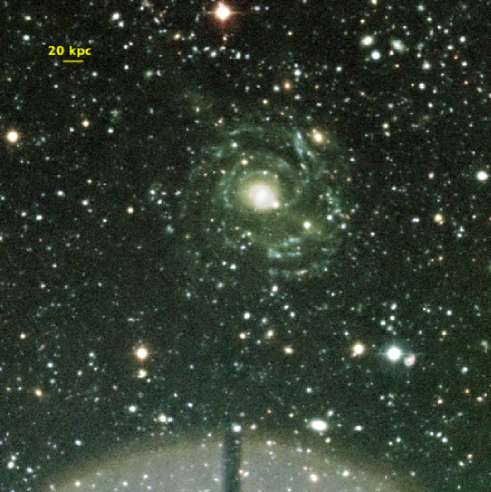
Figure 1: Color composite of the NGVS Malin 1 images ($u$, $g$, $i$, $z$ in blue, green, yellow, red, respectively). The image measures about 4.5 arcmin across (1 arcmin $\sim$ 107 kpc).

Table 1: Summary of the new observations presented in this work.

Filter	Wavelength	Exposure	PSF
	(Å)	time (s)	(arcsec)
GALEX $FUV$	1528	5030	5.00
GALEX $NUV$	2271	4662	5.00
CFHT MegaCam $u$	3550	6402	0.79
CFHT MegaCam $g$	4750	3170	0.85
CFHT MegaCam $i$	7760	2055	0.54
CFHT MegaCam $z$	9250	3850	0.59

2 Observations

2.1 New UV and optical images

In the $NUV$ and $FUV$ bands of GALEX, we use images from the GALEX Ultraviolet Virgo Cluster Survey, GUViCS (Boselli et al., 2011). The typical exposure time of one GALEX orbit (1500s) corresponds to a surface brightness limit of about 28.5 mag arcsec^-2. While Boissier et al. (2008) computed UV integrated magnitudes for Malin 1 using these data, in this paper we combine all GALEX tiles in which the galaxy is imaged to obtain an accumulated exposure time 3 times longer than in this previous work. To do so, we used the Montage software (Jacob et al., 2010) and resampled the data on same grid and pixel scale as the MegaCam images (in a similar manner as in Boissier et al., 2015), to facilitate the comparison between the UV and optical data. The GALEX PSF of the images is about 5 arcsec. Few foreground stars are present at these wavelengths, and they were manually masked. The value of masked pixels was estimated by interpolation from nearby pixels.

We also use images obtained by the NGVS (Ferrarese et al., 2012), in the $u$, $g$, $i$ $z$ bands. The survey reaches 29 mag arcsec^-2 in $g$. A color composite of these bands is shown in Fig. 1. Appendix A shows all the individual images used in this work at their native resolution. The NGVS images were processed with the Elixir-LSBG pipeline optimized for the recovery of low surface brightness features (see Ferrarese et al. 2012 for details). A bright foreground star is present at the South of the galaxy, producing a large halo (partly visible in Fig. 1) and causing a large-scale low surface brightness structure in the background. We fit a radial gradient to this structure, and subtracted it to flatten the images before analysis. We then used the point source catalog maintained by the NGVS collaboration to prepare a mask from the positions of objects marked as stars. This mask was visually inspected within the perimeter of the galaxy to mask additional stars and background galaxies or to unmask HII regions from the galaxy. In case of doubt, the objects were not masked. Masked areas were then replaced by interpolated values from the surrounding pixels.

Table 1 lists the final exposure times of the images, with their spatial resolution (about 5 arcsecs in the GALEX images, and measured on some of the numerous stars surrounding the galaxy in the NGVS images).

The NGVS images were convolved with a Gaussian filter in order to match the spatial resolution of the GALEX data,   5 arcsecs (all the results published thereafter are obtained within bins or regions larger than this size). Surface photometry (radial profiles and regions) was measured in these images, after correcting for a foreground Galaxy extinction with $A_{V}$=0.101 mag (from Schlafly & Finkbeiner, 2011, as found on the NASA Extragalactic Database). The sky level and dispersion was measured in all cases in a large number of small regions surrounding the galaxy.

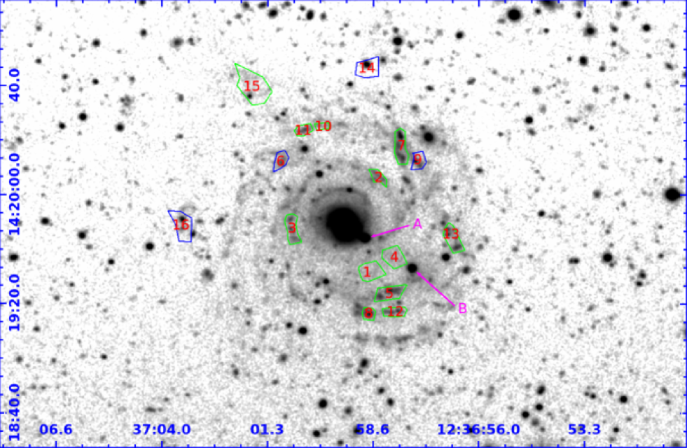
Figure 2: $g-$band image of Malin 1. Labels A and B, respectively, mark the position of Malin 1B, the nearby companion galaxy of Malin 1 identified by Reshetnikov et al. (2010) and of a likely background galaxy (Galaz et al., 2015). A few regions selected for additional analysis (see Sect. 4.1) are also shown (green delimited regions were selected in the $g-$band images, blue delimited regions were chosen in addition from the UV images, after the reduction described in Sect. 2.1). All the original images at their native resolution are shown in appendix A.

A simple examination of the final images already provides us with information concerning Malin1. First, the extended disk presents a clear spiral structure in its bluer bands. It is apparent in the $g$ band (Fig. 2), confirming the very recent result of Galaz et al. (2015). The spiral arms are similarly striking in the $u$ band. As Galaz et al. (2015), we also observe several diffuse areas such as the region marked 15 in Fig. 2. Region 1 has a brighter emission than the other inter-arm areas. It thus could be a feature produced during an interaction with Malin 1B that is not very far. Region 4, just next to it presents a similar level of emission. It is, however, located next to a background galaxy. Galaz et al. (2015) suggest that the elongated structure in the direction of region 4 is actually part of the background galaxy. Notice that they used specific data reduction techniques to enhance the detection of faint structures, and we refer to their work for a detailed morphological analysis.

Extended emission is also clearly seen in the $FUV$ and $NUV$ images (appendix A) even if the spiral arms are not as visible as in the optical, partly because the data are not as deep, and have a lower spatial resolution. Some areas emitting in the $u$ or $g$ band are clearly not emitting in $FUV$, and are weak (at best) in NUV. This could be a sign of episodic star formation. Regions formed less that 100 Myr still have massive stars emitting in $FUV$, while older regions no longer contain UV-bright stars.

2.2 Ancillary data concerning the gas and dust content of Malin 1

Lelli et al. (2010) have re-analyzed the Pickering et al. (1997) VLA observations of Malin1 to produce a HI surface density profile that we adopt for comparison to our models. We simply apply a 1.4 correction factor to convert it to the total neutral gas surface density. They also provide a rotation curve (albeit subject to uncertainties due to the inclination of the galaxy as will be discussed in the next section). Malin 1 was never detected in molecular gas tracers (Braine et al., 2000; Lee et al., 2014). We thus assume the molecular fraction is low in this very extended low density disk, as may be expected from the extrapolation of the trends found in nearby galaxies (Leroy et al., 2008) or in other low density regions (Dessauges-Zavadsky et al., 2014). For these reasons, we do not correct the gas profile for inclusion of molecular gas, bearing in mind this introduces a large uncertainty.

Proper estimations of the amount of dust attenuation or of the dust mass require the measurement of the far-infrared total emission (e.g., Cortese et al., 2008). Rahman et al. (2007) attempted to observe Malin 1 with Spitzer and obtained only upper limits at the longest wavelengths. They did have a detection at 24 microns, but their image shows that it only concerns the central part of the galaxy. The Virgo cluster was observed with Herschel in the context of the HeViCS survey (Davies et al., 2010). We inspected the images of this survey. Malin 1 is close to the edge of the survey but is within the observed area at 250 and 500 microns. Nothing is clearly detected in either of the corresponding images. The limits from the Spitzer observations were combined with integrated UV luminosity by Boissier et al. (2008) who estimated the FUV attenuation to be lower than 0.4 mag. LSBGs in general are believed to contain less (or colder) dust than their high surface brightness counterparts (Rahman et al., 2007; Hinz et al., 2007; Das et al., 2006)

3 Surface brightness profiles

3.1 Geometrical parameters

The surface brightness profiles can be measured easily once the geometrical parameters (inclination and position angle) are fixed. For Malin 1, values used as reference for these parameters in the literature are from Moore & Parker (2006) who matched manually an ellipse to their $R$ band image and found an axis ratio of 0.8 and a position angle of 43 $\deg$. It is possible to revisit the values of these parameters with our deep NGVS images. To do so, we used GALFIT (Peng et al., 2002) to fit 3 components (Sersic, exponential disk and a flat sky gradient) to each of the optical images. The center of the Sersic and exponential disk components were fixed and coincide with the peak of emission in the center of the optical images. Initial values were visually guessed for other parameters (position angle, axis ratio, effective radius) but varying them slightly does not change the results. GALFIT independently fits the three components in each band. The geometrical results of GALFIT are given in Table 2 with the uncertainties, as provided by GALFIT. We omit the sky component that is almost null and close to flat, but that we included in the fit in order to take into account possible residuals from the procedure we applied to subtract the background (especially the contribution from a nearby bright star, see Sect. 2.1). The resulting fits can also be seen in Fig. 3

input image	model	residual

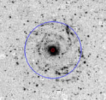
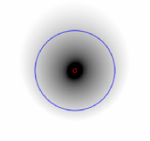
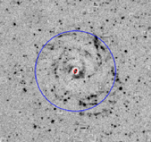
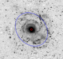
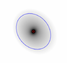
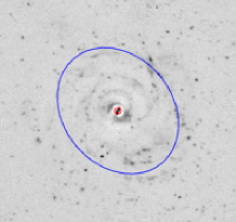
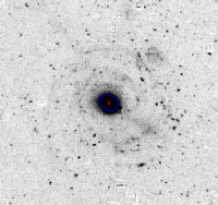
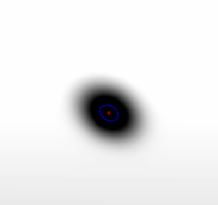
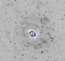
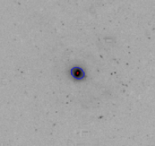
Figure 3: GALFIT results. On the left, we show the input image for GALFIT, in the middle its model, and on the right the residual. In each image, we show 2 ellipses indicating the geometry found by GALFIT in terms of effective radius, PA, axis ratio for the disk (outer blue ellipse) and the sersic component (inner red ellipse). From top to bottom: u, g, i z.

The results indicate that our simple fit finds an extended disk in the bluest bands ($u$, $g$), but fails to do so in the reddest bands ($i$, $z$) in which the extended disk (and the associated spiral arms) are less conspicuous and GALFIT instead fits inner structures that are more prominent. It is also clear from the residuals that the Sersic component fails to fit the inner region. This is not surprising considering the different structures found by Barth (2007): the bulge, bar, and disk that we have not attempted to reproduce. This may partly affect the parameters found for the extended disk even if it is well seen in the model images in the $u$ and $g$ bands. Technically, it would be possible to force GALFIT to fit more components (e.g., inner bulge, bar, and disk, spiral structure), or to keep a large radius for the disk component, but the rest of the paper does not depend strongly on these results (except for deciding on an axis ratio and PA for the ellipse procedure as detailed later). The outer disk is very weak in $z$ band and a proper determination would be in any case difficult. The PA and axis ratio found in the $u$ and $g$ bands are very similar to those of Moore & Parker (2006), even if the fit is consistent with a face-on orientation in $u$. The difference in apparent inclination could be related to the respective weight of the geometry of the spiral arms of the star forming extended disk, and the distribution of the old stellar populations, although it is probably affected by the different signal to noise in the two bands. The formal errors found by galfit are small, but they do not necessarily imply this solution is definitive. As a test, we attempted to fit respectively the $u$ and $z$ bands with the axis ratio and position angle derived from respectively the $z$ and $u$ bands. We found that GALFIT finds a solution in both cases without a significant increase of the $\chi^{2}$: the range of values found for the PA and axis ratio at various wavelengths are thus all consistent with our data. As a result, the real inclination is somewhat unconstrained. In this work, we computed surface brightness values for two inclination, one matching the geometry found in the $u$ band (showing well the extended star forming disk and the young stellar populations), and one corresponding to the geometry in the $g$ band (older stellar population, optimal quality data). Lelli et al. (2010) have found a warped HI disk in Malin 1. The very low surface density of the stellar disk, and the asymmetry of the spiral arm (the most visible regions at large radii) would make difficult the detection of a stellar warp with our data. Nevertheless, we adopt a third possible assumption for the geometry taking into account this possibility, inspired by Lelli et al. (2010), that is an axis ratio of 0.8 as previously, but a variable position angle (-1 degree for the inner 15 arcsecs, and rising with radius as 1.4 $\times$ the radius in arcsec beyond 15 arcsec, as given in Lelli et al. 2010).

Table 2: Galfit results.

Filter	Disk	Disk	Disk	Sersic	Sersic	Sersic	Sersic	reduced
	scalelength	b/a	PA	index	effective radius	b/a	PA	$\chi^{2}$
	(arcsec)		(deg)		(arcsec)		(deg)
u	23.23 $\pm$ 0.47	0.97 $\pm$ 0.01	NA	2.71 $\pm$ 0.03	2.07 $\pm$ 0.02	0.85 $\pm$ 0.01	-24.00 $\pm$ 1.14	1.148
g	25.26 $\pm$ 0.26	0.80 $\pm$ 0.01	40.26 $\pm$ 0.82	2.95 $\pm$ 0.01	2.192 $\pm$ 0.01	0.93 $\pm$ 0.01	-19.58 $\pm$ 0.99	1.155
i	3.88 $\pm$ 0.02	0.75 $\pm$ 0.01	57.07 $\pm$ 0.32	2.45 $\pm$ 0.01	0.96 $\pm$ 0.01	0.67 $\pm$ 0.01	-25.42 $\pm$ 0.17	1.377
z	3.74 $\pm$ 0.02	0.78 $\pm$ 0.01	56.79 $\pm$ 0.41	2.10 $\pm$ 0.01	0.95 $\pm$ 0.01	0.70 $\pm$ 0.01	-23.86 $\pm$ 0.17	1.343

3.2 Measurement of the surface brightness profiles

Figure 4 shows the $FUV$ to $z$ radial profiles of Malin 1, assuming the three sets of assumptions concerning the parameters (constant PA and slightly inclined with $b/a$=0.8, almost face-on with $b/a$=0.97, and variable PA with $b/a$=0.8). They are corrected for the $cos(inclination)$ factor to obtain face-on values. They were computed with the task ELLIPSE in IRAF, keeping the center fixed and computing the profiles in the same rings in each band. Error-bars were computed taking into account the uncertainty in the sky determination, combining the sky deviation itself (on a pixel basis), but also the deviation between several area of sky around the galaxy to account for residual structure in the background of the images, as presented in Gil de Paz & Madore (2005), which often dominates the error budget at low surface brightness in our images. The profiles present small differences but are mostly within the error-bars of each other. The real geometry may be a bit different from the 3 test-cases that we adopted, but our discussions and conclusions will remain unchanged in that case.

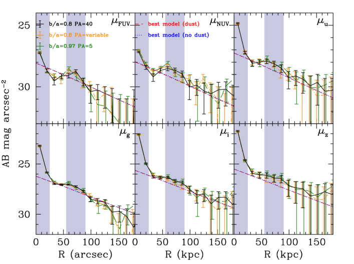
Figure 4: Surface brightness profiles for Malin 1 assuming three possible geometries (see legend in top-left panel): an axis ratio of 0.8 and a PA of 40 degrees, an axis ratio of 0.97 and a PA of 5 deg, or an axis ratio of 0.8 and a variable PA as suggested in Lelli et al. (2010). Profiles have been de-projected to their face-on value. They are compared to the best fit model of Sect. 5.1 including or not dust attenuation. The shaded area presents the regions excluded from the fit (avoiding the bulge and bumps likely related to the spiral structure) but the model is in agreement with the data also in the remaining of the disk (within a few sigma).

In our profiles in the $g$ and $i$ bands, we measure points above the noise level and with an approximate exponential radial distribution up to about 130 kpc.

4 Spectral energy distribution of regions of interest

A galaxy SED (even when azimuthally averaged at a given radius) will be a mixture of multiple generation of stars. Ideally, the detailed history of individual pixels can be assessed in nearby galaxies. However, due to the very low surface brightness of most of the disk, the signal per pixel is very low in a large part of the disk, making an analysis of the full map of the galaxy on a pixel basis difficult. In this section, we define 16 distinct regions that are readily visible in the optical or UV images and encompass enough pixels to increase the overall signal to noise ratio. This approach allows us to establish that the regions have not been formed simultaneously; rather, several distinct stellar populations appear to be present in the low surface brightness disk of Malin 1.

4.1 Measurements in 16 regions

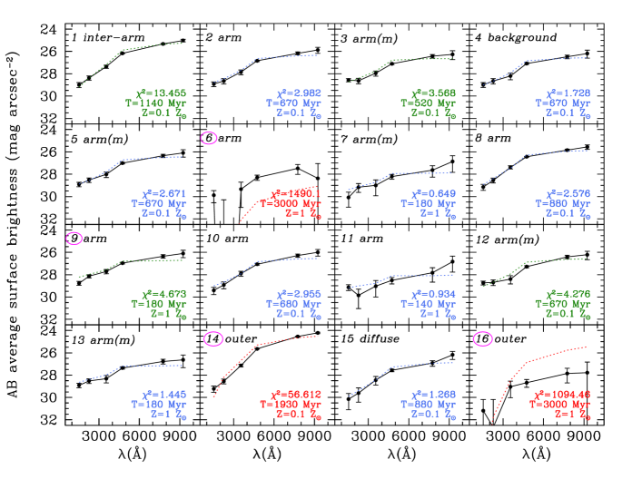
Figure 5: $FUV$ to $z$ SEDs for 16 selected regions (defined in Fig. 2 and in Section 4.1). The black lines with points and errorbars are the observed SEDs. The dotted line is the SED for the single generation fit (Sect. 4.2). The color indicates the quality of this fit: relatively good, average, bad fits are shown in blue, green and red, respectively, based on the $\chi^{2}$ value given in each panel. The number id of each region is circled for regions selected in ultra-violet, the other regions were chosen in the optical.

We defined 16 small regions manually by carefully inspecting the images at our disposal. We have not attempted to catalog every single region detected in a particular image, but have tried to cover the observed diversity of regions (spiral arms, inter-arm, diffuse area) and range in distance from the galactic center. The shape and position of the regions are shown in Fig. 2. Most regions were selected in the $g$ MegaCam image, many of them being part of the spiral structure visible in this image and in the $u-$band (2, 3, 5, 11, 8, 10, 7, 12, 13). Some of the regions (3, 5, 7, 12, 13) encompass several knots, but the knots have similar color and appearance within the selected region in that case. A few regions were selected as being diffuse in these images (1,4,15, some of them possibly resulting from past interactions, or linked to a background galaxy as discussed in Section 2). Some additional regions (6, 9, 14, 16) were chosen from the GALEX images on the basis of their relative high $FUV$ emission, but they were not obvious choices in the optical bands and had not been selected on their basis. All regions were defined manually, using the images matched to a common resolution and with contaminants having been removed. A summary of the characteristics of the regions is given in Table 3.

Aperture photometry was performed directly on the NGVS and GUViCS images (with masked objects interpolated over, and convolved to match the GUVICS resolution as for the surface brightness profiles) and we computed the average surface brightness in the 16 regions. The obtained SED are shown in Fig. 5.

4.2 SED fitting

In an attempt to establish the age of the last significant star-formation event, we use the colors of an aging stellar population from Boissier et al. (2008). They showed that the $FUV-NUV$ color reddens quickly after a brief ($10^{8}$ yr) epoch of star formation stops, and that the colors of various LSBGs are consistent with a succession of quiescent and active phases of star formation (the results were similar for a shorter or longer star forming episode). The same model predicts the magnitude in all bands, and instead of using only the $FUV-NUV$ color, we use here the full SED to try to constrain the age of the dominant population of each region. As in Boissier et al. (2008), we assume a Kroupa (2001) IMF, and that the last significant star forming event lasted $10^{8}$ yr. We interpolate metallicities in the range 0.1 to 1 solar, and ages up to 3 Gyr. Older ages are not physical for this single population assumption for which we assume the light is dominated by the ”last” star forming event, neglecting the underlying population that may include a broader range of ages.

The best fits are shown in Fig. 5 together with the $\chi^{2}$ values. Table 3 provides the results and the interval of confidence (one sigma). Globally, the metallicities are very poorly defined (the fit usually falls on one extrema, and all of the regions but two are consistent with 0.1 solar). Metallicities derived from fitting broad-band observations are known to have limitations (e.g., Gil de Paz & Madore, 2002). Ages are better constrained and are typically found in the range of a few hundred Myrs, with a clear spread (not all the regions in the spiral arms were formed simultaneously). The regions selected from their $FUV$ emission are usually poorly fit. Inspection of the SED suggests a blue $FUV-NUV$ color but red SED otherwise that cannot be fit with a single stellar population, suggestive of multiple populations.

The diffuse region 15 is consistent with stars born 0.9 Gyr ago (between 0.5 and 1.3 Gyr). This is consistent with the age of the interaction proposed by Reshetnikov et al. (2010) but among the spread of ages found in the other regions. The inter-arm regions 4 indicates a relatively young age (0.67 Gyr), while the nearby region 1 is older (1.14 Gyr), possibly indicating a different nature (region 4 could be part of a background galaxy according to Galaz et al., 2015).

Table 3: List of regions (ranked by distance to the center of the galaxy) and results of single age population fit.

ID	$\chi^{2}$	Age	Metallicity	Selected in	Comment
	reduced	(Gyr)	Solar	(band)
1	13.455	1.14 ( 0.87 - 1.16 )	0.10 ( 0.10 - 0.22 )	$g$	Diffuse inter-arm region
2	2.982	0.67 ( 0.58 - 0.82 )	0.10 ( 0.10 - 0.23 )	$g$	Single knot, spiral arm
3	3.568	0.52 ( 0.17 - 0.68 )	0.10 ( 0.10 - 1.00 )	$g$	Multiple knots, spiral arm
4	1.728	0.67 ( 0.46 - 0.77 )	0.10 ( 0.10 - 0.36 )	$g$	Diffuse inter-arm region (background?)
5	2.671	0.67 ( 0.48 - 0.75 )	0.10 ( 0.10 - 0.32 )	$g$	Multiple knots, spiral arm
6	1490	3.00 ( 2.72 - 3.00 )	1.00 ( 0.99 - 1.00 )	$FUV$	Single knot, spiral arm
7	0.649	0.18 ( 0.12 - 0.95 )	1.00 ( 0.10 - 1.00 )	$g$	Multiple knots, spiral arm
8	2.576	0.88 ( 0.78 - 0.93 )	0.10 ( 0.10- 0.20 )	$g$	Single knot, spiral arm
9	4.673	0.18 ( 0.17- 0.68 )	1.00 ( 0.10 - 1.00 )	$FUV$	Single knot, spiral arm
10	2.955	0.68 ( 0.57 - 0.95 )	0.10 ( 0.10 - 0.34 )	$g$	Single knot, spiral arm
11	0.934	0.14 ( 0.06 - 0.41 )	1.00 ( 0.10 - 1.00 )	$g$	Single knot, spiral arm
12	4.276	0.67 ( 0.41 - 0.73 )	0.10 ( 0.10 - 0.33 )	$g$	Multiple knots, spiral arm
13	1.445	0.18 ( 0.15 - 0.65 )	1.00 ( 0.10 - 1.00 )	$g$	Multiple knots, spiral arm
14	56.612	1.93 ( 1.84 - 1.94 )	0.10 ( 0.10 - 0.11 )	$FUV$	Single knot, outer region
15	1.268	0.88 ( 0.51 - 1.31 )	0.10 ( 0.10 - 0.61 )	$g$	Diffuse region
16	1094	3.00 ( 2.92 - 3.00 )	1.00 ( 1.00 - 1.00 )	$FUV$	Single knot, outer region

The approach based on this single stellar population is probably not realistic but is very simple (only 2 parameters). Although full star-formation histories cannot be derived using only six bands, we attempt in the appendix B to fit the SEDs with (slightly) more complex star-formation histories, using SED fitting tools available online through the GAZPAR interface. We also found with this method a diversity of ages or star-formation histories among the regions.

To summarize this section, the SED and the ages that we have derived using different approaches do not indicate a unique behavior. The age is not peaked at an unique value as would be the case if all (most) of the regions formed simultaneously, as would be if they were the result of a short-lived interaction between the galaxy and a companion. Of course, this concerns the behavior on relatively short-time scale of individual regions, and we will investigate in Sect. 5.1 the long-term smooth star-formation history on the basis of the radial profiles.

5 Discussion

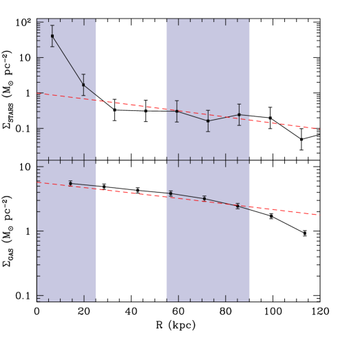
Figure 6: Top: Stellar mass density profile (points) computed on the basis of the surface brightness profiles (see Sect. 5.1.3). The error-bars indicate a factor two. Many uncertainties affect this profile such as the photometric errors, but also the model-dependent fit assuming a family of star-formation history, or an initial stellar mass function, so the factor of two is purely illustrative. Bottom: gas column density profile (points), converted from HI by multiplying by a factor 1.4 from Lelli et al. (2010). Error-bars are not provided by Lelli et al. (2010) so a 10 % uncertainty has been assumed. The shaded area indicates the regions excluded for the fit (based on the bulge and bumps observed in the photometric profiles) but the model is in agreement with the data also in the remaining of the disk. In both panels, the red dashed lines indicates our best model profile.

5.1 The large angular momentum hypothesis

5.1.1 Disk galaxy models

It was proposed that LSBGs are analogous to high surface brightness galaxies, but are simply more extended due to their larger angular momentum (Jimenez et al., 1998). This assumption was tested, for instance, by Boissier et al. (2003a) who modelled LSBGs with the same assumptions as adopted for the Milky Way and disk galaxies (Boissier & Prantzos, 1999, 2000), except for their larger spin parameter (a measure of the specific angular momentum). McGaugh & de Blok (1998) considered this possibility but found it unlikely to match the surface brightness distribution and the fact that LSBGs reside in low density environment. Boissier et al. (2003a) nevertheless showed that several LSBG properties are in agreement with this simple assumption. Here, we adopt this family of models, in the version presented in Muñoz-Mateos et al. (2011), with a Kroupa (2001) IMF. The models depend only on two parameters, the circular velocity ($V$) and the spin parameter ($\lambda$). They are characterized by scaling relationships such that the total mass of a galaxy scales with $V^{3}$, and the scale-length with $V\times\lambda$. The evolution at several radii is computed, neglecting any radial transfer. The star-formation rate density is computed from the local gas density as

$$\Sigma_{SFR}=0.00263\,\Sigma_{GAS}^{1.48}\,V/R,$$ (1)

where $\Sigma_{SFR}$ is expressed in M_⊙ pc^-2 Gyr^-1, $\Sigma_{GAS}$ in M_⊙ pc^-2, $V$ in km/s and $R$ in kpc. This star-formation law was chosen because it reproduces observations in nearby galaxies (Boissier et al., 2003b). The simulations of Bush et al. (2008) shows that spiral density waves can propagate in an extended low surface density disk allowing star formation even at large disk radii. The infall time-scale depends on mass and the surface density (dense regions are accreted early-on, massive galaxies are formed earlier than low mass galaxies). The models follow the chemical evolution of the disk, and calculate the resulting spectrum and colors. They also provide a computation of the dust attenuation, based on simple assumptions to estimate the amount of dust from the gas density and the metallicity. Since the assumptions concerning the dust role are very uncertain, we show our results with and without dust attenuation. However, at the very low density and metallicity considered here, the dust makes essentially no difference.

In this study of Malin 1, we need to extrapolate these models to much larger $\lambda$ values than it was done in previous studies. In Boissier et al. (2003a), the spin parameter was investigated up to $\sim$ 0.2. Malin 1 is an extreme case. We thus had to compute new models keeping all other assumptions identical, with very large values of the spin parameter (up to 0.7).

5.1.2 Best model for the extended disk of Malin 1

We computed $\chi^{2}$ in a very similar manner as Muñoz-Mateos et al. (2011) to determine the best fit parameters and their uncertainties. We performed this task within a radial range excluding the bumps clearly seen in the $FUV$ and $NUV$ profiles likely linked to the spiral arms (in which the excess of light from recent star formation can outshine the longer-term star-formation history), and the bulge (which is especially pronounced at the redder wavelengths). We thus fit the models to match two radial range: 20-35 and 65-100 kpc. Different choices for the radial range have very little consequence on our final results as long as the two central points are excluded. We performed the fit with three assumptions about the geometry as discussed in Section 3.1 and using the photomery alone, the gas profile alone, or both. The results are summarized in Table 4.

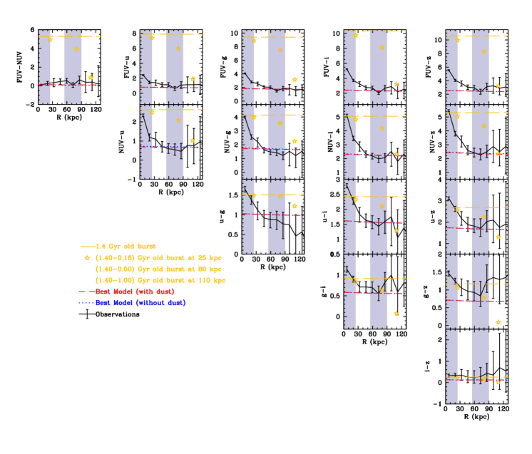
Figure 7: All the color indexes profiles we have access to, and comparison to model predictions. The top-left side shows the color sensitive to young stellar population, while the bottom-right colors are sensitive to older ones. We show the best model discussed in Sect. 5.1 (with our without dust) and the colors of a burst of age 1.4 Gyr (horizontal line), and different ages for different radii (stars). The shaded area show the regions excluded for the fit (bulge and bumps likely linked to the young populations of the spiral arm), but the color profile of the model is in full agreement with the observed one also in the remaining of the disk (within a few sigma).

Table 4: Best fitting models ($\chi^{2}$ based).

b/a	used	velocity (km/s)	spin
PA	constraints	(km/s)	parameter
0.97	photometry	490 (380 to 600)	0.61 (0.48 to 0.69)
N/A	gas	350 (340 to 360)	0.35 (0.32 to 0.39)
	both	420 (360 to 540)	0.54 (0.45 to 0.67)
0.8	photometry	430 (360 to 580)	0.57 (0.47 to 0.69)
40	gas	330 (320 to 340)	0.39 (0.35 to 0.43)
	both	380 (340 to 480)	0.51 (0.44 to 0.63)
0.8	photometry	460 ( 370 to 600 )	0.58 ( 0.48 to 0.69)
var	gas	330 ( 320 to 340)	0.39 ( 0.39 to 0.43)
	both	390 ( 350 to 390 )	0.51 ( 0.51 to 0.62)

Regardless of the assumptions we make, the profiles are best fit by a disk with a very large velocity and a very large spin parameter. We found that the lower limit of the parameters is better constrained (the $\chi^{2}$ increases quickly when moving towards lower values) than the upper limit. This is a strong constraint as it makes the extended disk of Malin 1 an extra-ordinary object, even if we adopt the lowest limit of the parameters interval allowed (i.e., a spin parameter larger than 0.3 and a velocity larger than 320 km/s). Since the gas profile does not include the molecular component (even if it is likely to be low) and has a lower spatial resolution, we prefer to adopt the parameters for the fit of the photometric profile alone (the table clearly shows that similar values are obtained in any case). With the geometry of $b/a$=0.8 and a constant PA, we obtain $V$=430 km/s and $\lambda$=0.57, that we consider our reference model in the following.

5.1.3 Observed and modeled profiles

The photometric profiles obtained for our best model are shown together with the observations in Fig. 4 and the gas profile with the observed one in Fig. 6. In this figure, we also show the stellar surface density of our best model. We compare it to the profile derived from the photometric profiles adopting the method of Roediger & Courteau (2015). The stellar mass to light ratio is estimated using the correlation found between the $i$-band mass to light ratio and $g$-$i$ color (Roediger & Courteau, 2015) based on the FSPS stellar population model (Conroy et al., 2009). We assumed exponentially-declining star-formation histories, and a wide range of metallicities and reddenings. Despite the different method, and even the different assumptions used (e.g., for the IMF and star-formation histories), this method and our model provide a consistent description of the stellar mass distribution in the giant disk of Malin 1.

Figure 7 shows the full set of color profiles obtained with our data. The short wavelength colors (e.g., FUV-NUV) suggest recent or current star-formation activity, as a relatively old burst alone could not explain the observed color. The colors in the redder bands (e.g., $i$-$z$) that are sensitive to the past history of star formation suggest this activity has persisted for some time in the past. Our best model indeed reproduces the flat color gradient within the disk, except in the inner 20 kpc that are dominated by the bulge (that we do not attempt to model). If we follow Barth (2007), the inner 20 kpc resembles a normal galaxy, while the rest of the galaxy is the largest XUV star forming disk ever seen, that is surprisingly well fit by a model entirely calibrated on usual disk galaxies such as the Milky Way. We recognize that even if the best model is consistent with the colors profiles (for almost all the points within one sigma error-bars), some discrepancies are visible. For instance, the $FUV-z$ observed profile is a bit redder than the model one, and we can suspect a gradient in the inner 60 kpc. One possibility is that the inner part of the galaxy actually extends further out than the 25 kpc that we adopted as a limit. We have not attempted to subtract the extrapolation of an inner component that may affect the colors. The effect would be stronger for colors involving red bands (blue colors such as $FUV-NUV$, $FUV-u$ are quite flat, while as soon as we involve a red band starting from $g$, the central component becomes more prominent). This would affect both the gradient and the absolute value. Some systematic shifts may have other origins. For instance, the model is globally too red by a few tenths in $u-g$, and too blue in $g-z$ and $g-i$, what could be due to errors in the estimation of the sky level in the $g$ band. Since we are at very low surface brightness, the sky level uncertainty plays a big role. Despite our best effort, we may have a systematic offset due to an error in its determination. Our error-bars, however, include an estimate on this source of error (by measuring the sky in different part of the image around the galaxy and estimating its large-scale variation), and indeed the models are within these error-bars. Finally, we used models with only 2 free parameters, while most of the galactic physics is fixed from previous works (e.g., the efficiency of star formation, the accretion history and its dependence on radius, the IMF). Some of the systematic differences could come from these assumptions (e.g., if the IMF varies slightly with density). By relaxing these assumptions, we could probably obtain better fits, but we would not learn much more about the galaxy.

Despite these small differences in colors, this simple model is consistent with the observed color profile, without fine-tuning outside of the two free parameters; and it predicts very different colors from other assumptions such as an old burst, or a star-formation ring expanding with time as discussed in Sect. 5.2.

5.1.4 Predictions concerning the History of the Malin 1 giant disk

Under the assumption that this model is correct, we can make some predictions on the history of the galaxy, and on its past and present metallicity (Fig. 8).

A long, protracted star-formation history is necessary to account for the galaxy’s large mass: the low stellar density and large spatial extent, combined with the adopted star-formation law, implies a low star-formation efficiency and a relatively modest star-formation rate that gradually builds up the disk of the galaxy over an extended period of time. This long history is also consistent with the kinetic information. Indeed, the HI kinematics is regular and symmetric, while the orbital time scale is extremely long ($\sim$ 3 Gyr). Then, the outer disk must have been in place and undisturbed for many Gyrs (Lelli et al., 2010). The resulting stellar mass to light ratio in the extended disk is low, as found in blue galaxies (see e.g., in Kauffmann et al., 2003; Gallazzi & Bell, 2009) with values of $log(M_{\star}/L)$ around $-0.45$ in the $u$ band, $-0.3$ in the $g$ band and $-0.2$ in the $i$ and $z$ bands. The baryonic mass (including gas) to light ratio instead rises from $log(M/L)\sim$ 0.4 to 0.7 between the center and R $\sim$ 100 kpc in the $u$ band (0.55 to 0.9 in $g$ band, 0.65 to 1 in $i$ and $z$ bands). This scenario also implies a low gas metallicity (slightly lower than 1/10 solar), which is consistent with the metallicities usually measured in LSBG, that are lower than in high surface brightness galaxies (e.g., McGaugh, 1994; de Blok & van der Hulst, 1998; Liang et al., 2010).

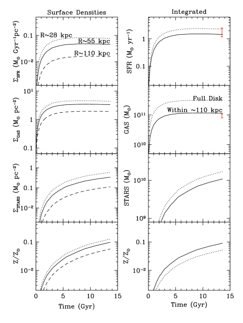
Figure 8: History of the extended disk in Malin 1 according to our best-fit model. Left: evolution at specific radii (28, 55, and 110 kpc). Right: evolution of integrated quantities (over the full disk modeled, or within about 110 kpc, corresponding to the size of the visible disk). The integrated values are compared to the values of Boissier et al. (2008) for the star-formation rate and Lelli et al. (2010) for the gas (shown by the errorbar in the topmost two right panels).

5.1.5 Discussion on the velocity and spin

Our reference model for the geometry of $b/a$=0.8 and a constant PA has for parameters $V$=430 km/s and $\lambda$=0.57 (similar values are found under the other geometries that we have tested). This velocity is much higher than the circular velocity found by Lelli et al. (2010) ($V\approx$220 km/s from the HI kinematics) although they adopted a similar inclination. This inclination is, however, quite uncertain since it is based purely on a manual fit of an ellipse to the $R$ band image of Moore & Parker (2006). Even a very small error on the inclination would translate in a large error in the velocity since the galaxy is almost face-on. As a result, the velocity of Lelli et al. (2010) is itself very uncertain. If the disk is more inclined than assumed by Lelli et al. (2010), then the velocity should be corrected for the different inclination. They adopted an inclination of 38 degrees. If the inclination is in fact 14 degrees (corresponding to the axis ratio of 0.97 that was measured in the $u$ band), the velocity of Lelli et al. (2010) corrected for the inclination becomes 564 km/s. Our best model is then instead $V$=490 km/s and $\lambda$=0.61 (likely in the range 0.35-0.7). A giant rotating disk with velocity in the range 300 to 500 km/s and spin in the range 0.35-0.7 is thus consistent with all the observations. This velocity is consistent with the observations of Lelli et al. (2010) only if the inclination is 18 degrees (instead of the 38 degrees they assumed). Galaxies with velocities around 300-400 kms/s are rare at best. Some may exist if we take at face values the velocity functions of Gonzalez et al. (2000) who combined luminosity functions and Tully-Fisher relations, and no galaxies are known with velocity larger than 300 (Lelli et al., 2016, from resolved rotation curves of 175 galaxies) or 400 km/s (from the HI line-width of the 4315 detections in the HIPASS catalog by Zwaan et al., 2010).

The spin parameter is also extremely large. For comparison, the properties of the Milky Way are well reproduced by a model with $V$ $\sim$ 220 km/s and $\lambda\sim$ 0.03, and Muñoz-Mateos et al. (2011) showed that the photometric profiles of 42 spiral galaxies of the SINGS sample were well reproduced using the same models with velocities in the range 50 - 300 km/s, and $\lambda$ in the range 0.02 - 0.08 except for two galaxies with $\lambda$ $\sim$ 0.14. For a larger number of galaxies but with a different method, Hernandez & Cervantes-Sodi (2006) also found a very similar spin parameter distribution.

The fact that Malin 1 requires extreme values to be fit may not be that surprising, since we already know that it is the most extreme galaxy for instance in central surface brightness and scale-length (see Fig. 7 of Hagen et al., 2016). We should thus keep in mind the possibility that we need an extended range of physical parameters with respect to other galaxies. On the other hand, these extremely large values suggest that this model may not be physical. Indeed the model implements scaling relations (between velocity, spin parameters, mass and scale-lengths) that may break down for the extended disk. Figure 9 indicates that it might be the case since the velocity that we obtained with our fit is too large for the galaxy as a whole to be on the Tully Fisher relationship (either the stellar one, or the baryonic one, probably more appropriate for this gas rich galaxy). The stellar mass was estimated by summing the stellar mass we measure in the extended disk, and the stellar mass in the inner disk as derived from the magnitude published in Barth (2007) combined with the stellar mass to light ratio in the R band of 3.3 of Lelli et al. (2010). For the baryonic relation, the mass of gas that needs to be added is obtained by multiplying the HI mass of Lelli et al. (2010) by a 1.4 factor to take into account other species. The largest velocities suggested by our fit is indeed too large with respect to the baryonic Tully Fisher relationship, unless Malin 1 is an outlier. Intermediate values around 300 km/s would still agree well with the relationship.

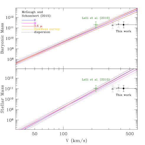
Figure 9: Stellar and Baryonic Tully-Fisher relationships taken from McGaugh & Schombert (2015). The different lines indicate different samples and wavelengths used in their work. The position of Malin 1 for the $\sim$ 220 km/s reported in Lelli et al. (2010) is indicated, as well as the “velocity” derived from our model fit (filled circle, open triangle, and open square for respectively the fit based on the photomeric profiles, the gas profile, and both).

If this is a good indication that the usual scaling laws break down in the extended disk of Malin 1, then the velocity and the angular momentum corresponding to the best fit loose their physical sense. The relative success of our model still may indicate that the extended disk of Malin 1 behaves like it is expected for a normal disk of low density : i) the model produces a correct star-formation law for the observed densities and radius, ii) it produces a correct star-formation history with right colors and stellar light density, iii) the extended disk follow an about exponential distribution.

We also made some ad-hoc models to understand the role of diverse assumptions in our results. We fixed the total surface density radial profile from the stellar and gas profiles (as seen in Fig. 6), and the rotation curve to be the one derived by Lelli et al. (2010) instead of using the scaling laws. Using the same star-formation law, and dependence of the accretion history on the velocity and surface density as in previous models, we found that the model does not provide a good fit to the data. While the gas profile is very similar to the observed one, we find two discrepancies: 1) the model under-estimates the surface brightness at radii larger than about 100 kpc (by more than 1 mag at 120 kpc), 2) the model predicts systematically bluer colors than the observed ones. Point 2 is related to the accretion history that we have adopted, corresponding to the low density and a velocity of about 200 km/s: most of the accretion occurs very late in the history of the galaxy. The light is then dominated by very young blue stars. We performed new computations with various accretion histories (taken from the usual models for different velocities), and various star formation efficiencies (adding a multiplying factor in equation 1). The colors are systematically improved when the accretion occurs earlier than in the first model. Modifying the efficiency has little effect on the colors. The best model is found by adopting a reduced efficiency (using a factor 0.5) but a very low efficiency (a factor lower than 0.3) and a very large one (larger than 1.5) are excluded. The star-formation law of equation 1 being deduced from data in which the scatter is close to a factor 2, this deviation in efficiency does not significantly distinguish Malin 1 from regular galaxies. Concerning the point 1, surface brightness profiles in better agreement with the data could be obtained by rising the star-formation efficiency with radius, but it is not clear on which physical basis this should occur. Another possibility is that our census of stars and gas is incomplete (e.g., wrong $M/L$ ratios, hidden gas at large radii). We tested this by correcting the total surface density by a factor corresponding to the difference in surface brightness between our best ad-hoc model and the observations, and running the grid of models again. The surface brightness profiles were improved, but the gas profile was then poorly fit. The color profiles were almost identical as in the previous set of models. Finally, all of the models constructed by imposing the observed surface density profile and rotation curve have worse $\chi^{2}$ than the one presented before. This is probably because the scaling relations with $V$ and $\lambda$ allowed us to explore a larger variety of surface densities, and thus of star-formation histories. The main conclusion of these tests is that an early accretion of the extended disk of Malin 1 is always favored. This is consistent with the other indications of a relatively long history of the giant disk as discussed before.

5.2 Ring galaxies and LSBGs

Mapelli et al. (2008) proposed that ring galaxies could be the ancestor of LSBGs. Ring galaxies exhibit a peak moving progressively outwards with time in their surface brightness profiles (Vorobyov & Bizyaev, 2003). The simulations of Mapelli et al. (2008) suggest that galaxy collisions indeed create rings that are visible up to about 0.5 Gyr after the interaction. They propose a model for Malin 1 where the collision occurred 1.4 Gyr ago for the galaxy to have the time to expand to such a size and the ring to dissolve into a large disk. Their work was based on a comparison with the Moore & Parker (2006) data. In our new surface photometry profiles, we do not see the typical features in the stellar density profile that they predict, such as a break around 50 kpc. In our images (Fig. 1 and appendix A), we do not see any sign of stellar ”spokes” like those seen in the Fig. 4 of Mapelli et al. (2008) for their detailed model of Malin 1, or for other LSBGs (such features are not visible in the $g-$ and $r-$band images of Galaz et al., 2015, either, even if the authors applied special techniques to enhance the contrast of structures). Some significant number of stars should also have been created during the ring phase. Even if they do not dominate the stellar population, they should have left some traces in the images, in the profiles, or in the SEDs of some regions including stars created at that time.

In Fig. 7, we placed a horizontal line corresponding to the color of a 1.4 Gyr old burst, adopting the Boissier et al. (2008) simple model for the colors of aging stellar populations. In their scenario, Mapelli et al. (2008) suggest the ring is located at about 25, 80, and 110 kpc, respectively, 0.16, 0.5 and 1 Gyr after the interaction. We thus indicate in the same figure the color expected for the remnant of the stars formed at that times, assuming they still dominate the stellar light at the corresponding radius. Clearly, the color profiles in Malin 1 are not in good agreement with this scenario. If stars were formed during the collision and the ring phase, they have left no obvious traces in the images or in the profiles. The ages of individual regions that we defined and fit with a single stellar population (or with more complex star-formation histories) in Sect. 4 are spread over a large range of values that do not agree particularly well with the ages expected based on the model.

We thus conclude that the color gradient in Malin 1 is not consistent with the progenitor being a ring galaxy. Instead, a long-term low efficiency formation of stars in a large disk, as presented in the previous section, is more likely.

5.3 Intermittent star-formation histories

The fits of selected regions along the spiral arms suggest different ages, spread over several 100 Myr, with signs of older stellar population (several regions e.g., 6,14,16) have red SEDs that are not well fit by a single recent population). We found no age gradient to which the spread of ages could be correlated.

This may indicate that, while the general model discussed in Section 5.1 represents the long-term regular history of the galaxy, the recent evolution is characterized by quiescent and active star-formation periods (so that we find regions in these different phases), as was suggested from the $FUV-NUV$ integrated color of a sample of LSBG galaxies in Boissier et al. (2008). Variations in the star-formation histories could also explain the existence of optically red LSBGs (Boissier et al., 2003a). The fact that some regions are blue in $FUV-NUV$ but red in other colors could also be explained if the blue color is due to a recent event of star formation in the last 100 Myr (contributing mostly to $FUV$), while the star formation on NUV emission time-scale (500 Myr) was lower, and if a significant amount of stars was formed at earlier epochs.

An optical spectrum with an estimate of the H$\alpha$ emission is available only for the center of the galaxy (Impey & Bothun, 1989). It would be extremely interesting to obtain new data on line emission in the galaxy to test the micro-variations of the star-formation history on time scales shorter than 100 Myr. New instruments, such as MUSE, with excellent efficiency and sufficiently large field of view should allow us to achieve this goal soon.

Our results then globally indicate that the properties of the extended disk of Malin 1 are consistent with a long history of low level star formation, with increased activity at some epochs in different regions, separated by phases that can last several 100 Myr. This is quite consistent with the analysis of the stellar populations in a sample of LSBG galaxies performed by Schombert & McGaugh (2014), and with the results of Zhong et al. (2010) for blue LSBGs. From HST data, Vallenari et al. (2005) also found that UGC5889, another LSBG has experienced modest bursts and very quiescent periods. Such a scenario for the star-formation histories is also suggested by the N-body simulations of Gerritsen & de Blok (1999).

6 Conclusion

We present a panchromatic view of Malin 1 based on deep UV-optical images from the NGVS and GUViCS surveys. The six photometric bands ($FUV$, $NUV$, $u$, $g$, $i$, $z$) used in our analysis are crucial for determining the stellar population of the galaxy and have allowed us to reach several notable conclusions concerning the properties of this prototypical low surface brightness giant galaxy.

• The extended disk of Malin 1 is consistent with a long standing disk that has been forming stars with a low star-formation efficiency.

• This low surface brightness disk is well fit by a simple model of evolution of disk galaxies. In this model the only significant difference with the Milky Way is the angular momentum, that is exceptionally large in the case of Malin 1: its spin parameter about 20 times larger than that of the Milky Way. The model however relies on scaling relationships that may break down in the extended disk of Malin1. The large velocities and spin parameter obtained may in that case loose their physical meaning. The predicted evolution could, however, still apply to the low density disk. This model allows us to make predictions on the stellar population of the galaxy, and the metallicity of the disk. Such predictions are testable by future observations. To maximize the consistency with the observations, we suggest the inclination of the galaxy could be around 18 degrees (or lower than 40 degrees often adopted in the literature) although this value is not strongly constrained.

• The stellar disk of Malin 1 extends at least out to 130 kpc in radius, confirming Malin 1 as a candidate for the title of largest known galaxy in the universe (and leaving open the question about how such large structures can survive during the hierarchical evolution of structures in a cold dark matter dominated universe).

• The morphological structure and colors of the extended disk in Malin 1 show no evidence of Malin 1 having a ring galaxy as ancestor, as previously suggested.

• Intermittent star-formation histories are favored by the colors of individual regions, as was suggested in some previous work on LSBGs.

Some of the conclusions reached in this paper could apply to other giant LSBGs, Malin 1 being the most spectacular case of this class of galaxy (although our current census of Malin 1 analogs in the local volume may be incomplete, Impey & Bothun, 1989). Likewise, some findings may be relevant to the numerous XUV disks found around normal disk galaxies (Thilker et al., 2007).

Appendix A Panchromatic images of Malin 1 at their native resolution.

Figures 10 to 15 show the six images at their native resolution.

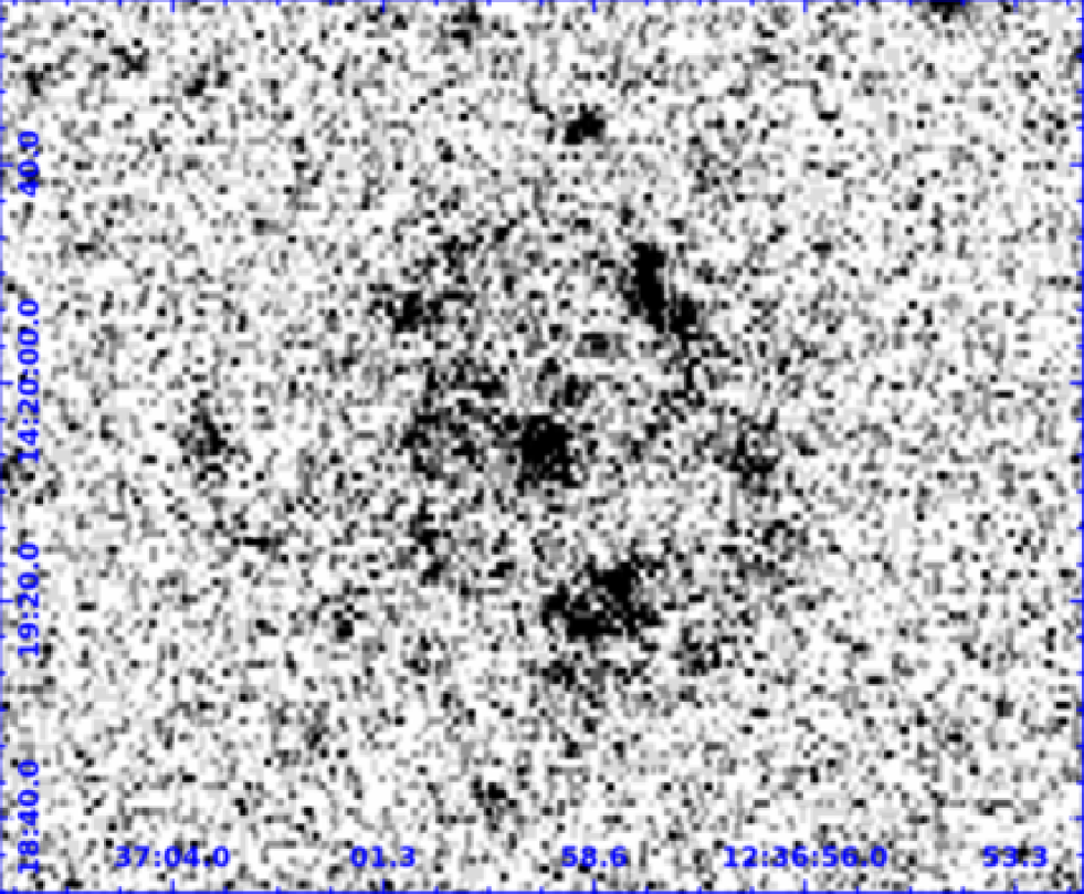
Figure 10: $FUV$-band image.

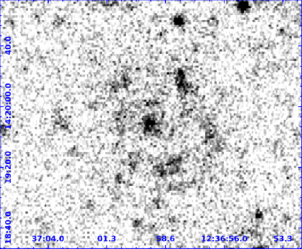
Figure 11: $NUV$-band image.

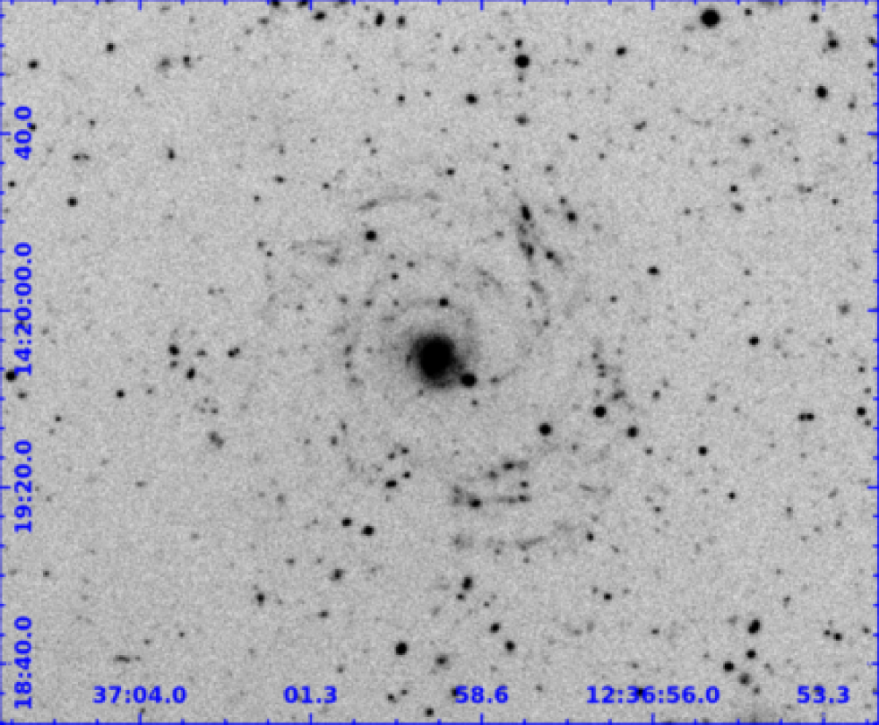
Figure 12: $u$-band image.

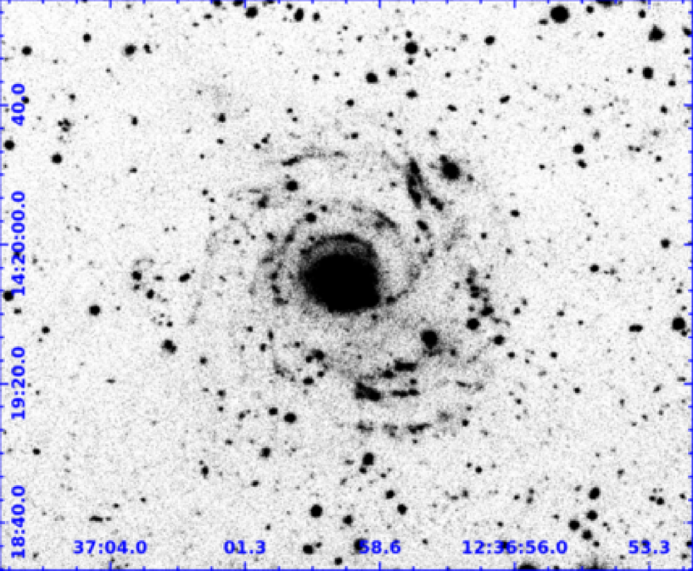
Figure 13: $g$-band image.

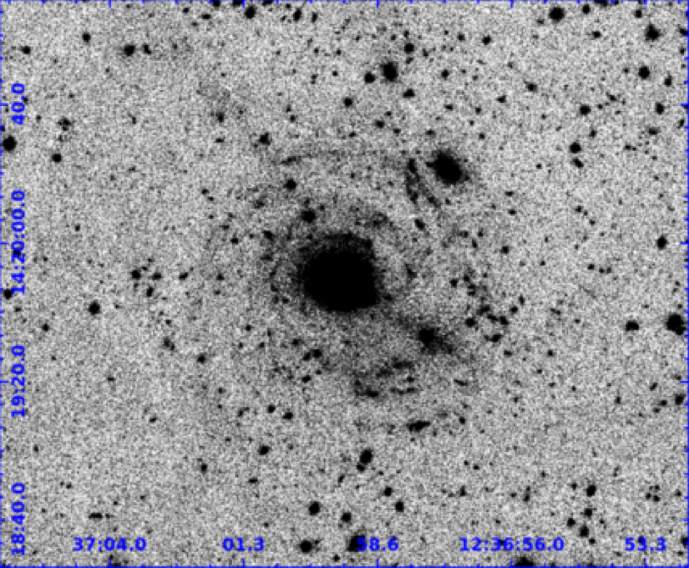
Figure 14: $i$-band image.

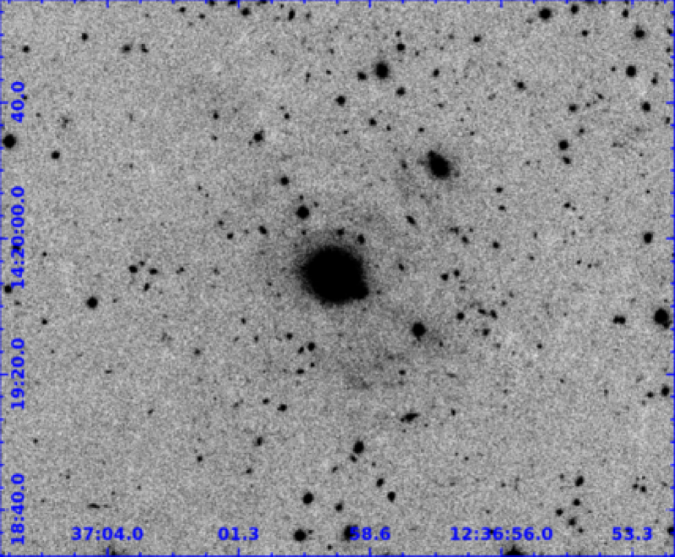
Figure 15: $z$-band image.

Appendix B GAZPAR modeling of the 16 regions spectral energy distributions.

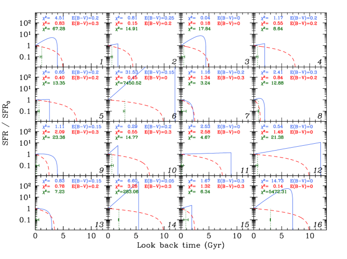
Figure 16: Star-formation history of individual regions for different models. The vertical dotted line indicates the age of a single population. The error-bar indicates the uncertainty on the age. The red dashed curve indicates the best star-formation history found by CIGALE. The blue solid curve indicates the best star-formation history found by Le Phare. In each panel, the non-reduced $\chi^{2}$ is given (from top to bottom: Le Phare, CIGALE, single generation). In the first two cases, the fit allows for the presence of dust, and the reddening of the best model is also given.

GAZPAR allows us to fit the SEDs of the regions selected in Malin 1 using two tools widely used in the community to compute for instance photometric redshifts or physical parameters, proposing different level of choices for various parameters and assumptions.

We first used GAZPAR to fit our data to Le Phare-Physical parameters. General presentations of this code can be found in Arnouts et al. (1999); Ilbert et al. (2006). The SEDs are fit with standard templates corresponding to Bruzual & Charlot (BC03) single stellar populations combined with a set of diverse star-formation histories (exponentially declining or delayed), a Chabrier IMF, $E(B-V)$ from 0 to 0.3 in 0.05 steps. GAZPAR uses the Chabrier IMF, while the models discussed in the main part of this work use the Kroupa (2001) IMF. However both IMFs are very similar for our purpose.

We then submitted the same catalog to the CIGALE code through the same interface. General information on CIGALE can be found in Burgarella et al. (2005) and Noll et al. (2009). We also use BC03 stellar population and Chabrier IMF. We choose delayed star-formation histories for which ages and time-scales have to be defined by the user. We allowed a large number of values for the timescale (in Myr): 10, 20, 50, 100 to 1000 in steps of 100, 1000 to 2000 in steps of 200, 2000 to 5000 in steps of 500, creating a variety of star-formation histories. We allowed the same values for possible ages, with the addition of even older ages (7500, 10000) to allow for stellar populations spread over a large range of ages. CIGALE allows the choice of a low metallicity (0.004), which we adopted since LSBGs are likely to be un-evolved (McGaugh 1994; de Blok & van der Hulst 1998; Burkholder et al. 2001; Liang et al. 2010). No metallicity data are however available for Malin 1 yet.

The results of both methods are show in Fig. 16 where we also indicated the age obtained in Sect. 3 for a single star forming event.

We remark that the two GAZPAR codes allowing to fit for an attenuation are in a surprisingly good agreement for this parameter in most regions. This does not necessarily imply that the result is telling us about the dust (both codes are based on similar principles, and they could use attenuation as a free parameter to compensate for other short-comings of our approach). However it suggests the regions with largest attenuation ($E(B-V)\sim$ 0.2 - 0.3) found by both codes (regions 1, 7, 8, 10, 15) could be interesting for future observations of the far infrared dust emission, or of molecular gas tracers.

In most regions, the two GAZPAR codes provide a consistent star-formation history. It indicates for several of them (1, 8, 9, 13, 15) short ages (and/or an increasing star-formation history with time). In all of the regions, the age derived in the simpler model of a fading burst is shorter than the age derived by the more complex star-formation history. All of this indicates that the luminosity of these regions is dominated by recent star formation. The two GAZPAR codes also agree in several regions to suggest an extended star-formation history (6, 11, 12, 14, 16) showing that a relatively old stellar population exists. This is true for regions 6, 14, 16 that were chosen as blue from their $FUV$ emission. The $\chi^{2}$ for those regions are not good in any scenarios. The blue $FUV-NUV$ color could be due to a recent and weak star forming event, on top of an old underlying stellar population responsible for the red optical colors that are indeed visible in Fig. 5. In some regions, the two codes provide different histories — a declining star-formation history, but of young age for Le Phare, and a rising star-formation history for CIGALE. This is likely due to regions where the light is dominated by a relatively young stellar population (less than few Gyr) as both scenarios indicate a high number of young stars.