Spiral order from orientationally correlated random bonds in classical $XY$ models

Abstract

We discuss the stability of ferromagnetic long-range order in three-dimensional classical $XY$ ferromagnets upon substitution of a small subset of equally oriented bonds by impurity bonds, on which the ferromagnetic exchange $J^{\,}_{\perp}>0$ is replaced by a strong antiferromagnetic coupling $J^{\,}_{\mathrm{imp}}<0$. In the impurity-free limit, the effective low-energy Hamiltonian is that of spin waves. In the presence of a single, sufficiently strongly frustrating impurity bond, the ground state is two-fold degenerate, corresponding to either clockwise or anticlockwise canting of the spins in the vicinity of the impurity bond. For a small, but finite concentration of impurity bonds, the effective low-energy Hamiltonian is that of Ising variables encoding the sense of rotation of the local canting around the impurities. Those degrees of freedom interact pairwise through a dipolar interaction mediated by spin waves. A spatially random distribution of impurities leads to a ferromagnetic Ising ground state, which indicates the instability of the $XY$ ferromagnet towards a spiral state, with wave vector and transition temperature both proportional to the concentration of impurity bonds. This mechanism of “spiral order by disorder” is relevant for magnetic materials such as YBaCuFeO₅, for which our theory predicts a ratio between the spiral ordering temperature and the modulus of the spiral wavevector close to the measured ones.

I Introduction

Insulating magnets supporting long-range magnetic spiral order are of technological interest as they can display “magnetically” induced ferroelectricity Katsura et al. (2005); Cheong and Mostovoy (2007); Khomskii (2009); Tokura and Seki (2010). In prototypical spin-spiral multiferroics, e.g., RMnO₃ (R=Tb³⁺, Dy³⁺, etc.) Kenzelmann et al. (2005); Goto et al. (2004), a magnetic spiral phase can be stabilized by the competition between nearest-neighbor and further-neighbor magnetic exchange interactions with opposite signs Mochizuki and Furukawa (2009); Lyons and Kaplan (1960). However, the resulting frustration only induces spiral states if further-neighbor couplings are sufficiently strong as compared to nearest-neighbor couplings. The latter are typically much bigger in magnitude, except under special circumstances that lead to their suppression. In such exceptional cases, the characteristic exchange scale is set by the further-neighbor interactions and is thus very weak, entailing a low spiral ordering temperature.

In order to engineer magnetic insulators with magnetic spiral order establishing at high temperatures, it is of fundamental interest to investigate analogous mechanisms. An interesting route was suggested by the study of Ivanov et al. Ivanov et al. (1996) who considered a Heisenberg antiferromagnet on a square lattice, in which every other horizontal nearest-neighbor bond in a staggered pattern was replaced by a ferromagnetic coupling. Sufficiently strongly frustrating bonds were shown to induce a magnetic spiral order. From the experimental side, there are interesting hints that a similar mechanism might be tied to the presence of disorder. Indeed, certain insulating compounds containing some degree of chemical disorder were reported to stabilize magnetic spiral order Cox et al. (1963); Utsumi et al. (2007); Morin et al. (2015, 2016); Kundys et al. (2009) at high temperatures. For example, the transition temperatures to the magnetic spiral phase were found to range from 180 K to 310 K Kundys et al. (2009); Morin et al. (2015); Caignaert et al. (1995); Kawamura et al. (2010); Ruiz-Aragón et al. (1998) in YBaCuFeO₅, whereby several further characteristics of the spiral depend on the degree of disorder. This empiric observation suggests the possibility that, for some materials, a magnetic spiral order might be induced by some “impurity bonds” formed by nearest-neighbor magnetic ions whose exchange coupling frustrates the order that would establish in their absence. Recent Monte Carlo simulations have confirmed this conjecture in a model describing YBaCuFeO₅ with disorder in the spatial location of the magnetic Cu and Fe ions Scaramucci et al. (2018). The latter was assumed to result in a small concentration of locally frustrating bonds along the $c$-direction, which indeed was shown to induce magnetic spiral order in an experimentally relevant window of parameters.

In this paper, we describe and study the general mechanism that renders the ferromagnetic long-range order of classical $XY$ spins unstable towards spiral order, when a finite fraction of the ferromagnetic interactions is replaced by sufficiently strong antiferromagnetic exchange couplings. In the end, we will confront the theory with experimental data, as shown in Fig. 1, with good quantitative agreement.

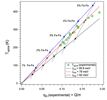
Figure 1: (Color online) Experimental data (circles) from Ref. Morin et al., 2016 for the compound YBaCuFeO₅, obtained by different annealing rates that control the fraction of bipyramids hosting magnetically frustrating Fe-Fe pairs instead of low energy Fe-Cu pairs. The transition temperature to the spiral state is plotted versus the spiral wavevector measured at low temperature. Our theory explains the linear relationship between the two and predicts the slope as a function of the three exchange couplings. We plot the predicted slope for different values of the exchange on the driving frustrating bonds, fixing the other two exchanges to the values estimated in Ref. Scaramucci et al., 2018. The larger the frustrating coupling, and the higher the fraction of frustrating Fe-Fe bonds in the bipyramids of YBaCuFeO₅, the larger the transition temperature and the spiral wavevector. Each triplet of triangular symbols joined by a dashed line corresponds to the same concentration of frustrating bonds in our theory.

The general physical mechanism at work is the following. We consider a geometrically unfrustrated lattice $\Lambda$ in $d>2$ dimensions, hosting isotropic spins with a continuous symmetry. The symmetry is broken spontaneously at low temperatures, which implies the existence of Goldstone modes. Dilute but strong impurity bonds embedded in this lattice can induce local cantings which behave as “dipole type” defects with an Ising degree of freedom associated to them. The Goldstone modes mediate an interaction between the defects, decaying as $r^{-d}$ for large separation. Correlations in the distribution of such impurity bonds (e.g., a restriction to bonds that point in a single direction) may ensure a sufficiently non-frustrated pairwise interaction between these defects so as to favor long-range ferromagnetic order in the orientation of the local cantings. Such long-range Ising order entails a global twist of the ferromagnetic order parameter density, and thus a magnetic spiral, as the local magnetization twists in the same sense across every impurity bond. The wave vector of the resulting magnetic spiral is proportional to the magnetization density of the Ising degrees of freedom, and thus, to the density of impurity bonds. We will show that such a spiral state is the ground state of the $XY$ system for a rather wide range of parameters of the impurity bond distribution.

For simplicity, we consider a cubic host lattice $\Lambda$ embedded in three-dimensional Euclidean space with the Cartesian coordinates $x$, $y$, and $z$. We impose a tetragonal symmetry by choosing the ferromagnetic nearest-neighbor exchange to be $J^{\,}_{\parallel}>0$ for couplings in the $x$-$y$ plane and $J^{\,}_{\perp}>0$ for bonds oriented along the $z$-axis. We further consider a set of impurity bonds, which form a dilute subset of the nearest-neighbor bonds that are directed along the $c$-direction of the cubic host lattice $\Lambda$. For each impurity bond, the ferromagnetic $J^{\,}_{\perp}>0$ is replaced by the antiferromagnetic exchange coupling $J^{\,}_{\mathrm{imp}}<0$.

A single impurity bond does not destroy the ferromagnetic long-range order of the ground state. However, it does result in a canting of the classical $XY$ spins in the vicinity of the impurity bond, provided that the local frustration is sufficiently strong, i.e., $|J^{\,}_{\mathrm{imp}}|\geq J^{\,}_{\mathrm{c}}$ for some threshold value $J^{\,}_{\mathrm{c}}>0$. Under these conditions (and with fixed boundary conditions at infinity) the ground state is two-fold degenerate, exhibiting either a clockwise or counter-clockwise sense of the local canting. At low concentration we can thus associate a corresponding low-energy Ising degree of freedom to every impurity bond. Apart from these discrete soft degrees of freedom, the background ferromagnet hosts low-energy spin wave excitations. They mediate an effective interaction between the Ising degrees of freedom, which results in an effective classical Ising model with effective two-body interactions of dipolar type. Their algebraic decay at large distance is a direct consequence of the gaplessness of the spin waves. A similar effective interaction results in any system that spontaneously breaks a continuous symmetry, and thus hosts gapless Goldstone modes mediating algebraic interactions between impurity degrees of freedom. The specific case where the impurity bonds form a Bravais superlattice, with a unit cell that is large compared to that of the cubic host lattice $\Lambda$, is analytically tractable, and for certain classes of superlattices we are able to rigorously establish the presence of spiral order.

Although the analysis in this paper assumes ferromagnetic interactions for the host lattice $\Lambda$, we note that our results can be readily extended to any unfrustrated $XY$ magnet. For example, if the lattice is bipartite and $J^{\,}_{\mathrm{imp}}$ has sign opposite to $J^{\,}_{\perp}$, the system can be mapped to the above described ferromagnet as follows. For every spin, a reference frame is chosen such that the unfrustrated ground state of the impurity-free system corresponds to a ferromagnetic configuration. By virtue of this mapping, the low energy effective theory presented below extends to this larger class of magnetic insulators.

We emphasize that for the establishment of ferromagnetic order it is central that the impurity bonds be not randomly oriented. Otherwise, the pair-wise interactions between the associated Ising degrees of freedom would be strongly random in sign, which would most likely lead to spin glass order, as observed in models of dilute, randomly oriented Ising dipoles Alonso and Fernández (2010); Fernández and Alonso (2009). Since an Ising glass state generally carries no net magnetization, it would not induce a spiral state of the original $XY$ spins. Also, in the limit of a high density of randomly oriented impurity bonds, one expects long-range spin-glass order (observed directly at the level of the $XY$ spins), since the model becomes that of a random-bond $XY$ gauge glass, as was studied by Villain Villain (1975, 1977, 1978).

The remainder of this paper is structured as follows. In Section II, we define the spin lattice model. Section III begins with the case of a single impurity bond. We then consider a small concentration of impurity bonds and derive a mapping to an effective Ising model for low energies. Section IV describes how to find the ground state of the effective Ising model when the impurity bonds realize a superlattice. The effective Ising model is solved by analytical and numerical means. Its solution is then compared to Monte Carlo simulations of a model with the same network of exchange interactions, but in which the classical $XY$ spins are replaced by classical Heisenberg spins with an additional easy-plane anisotropy. The latter allows for close contact with experimentally realized magnets, such as YBaCuFeO₅, which are believed to embody the physical ingredients and mechanisms discussed above. In Section V, we study the analytically tractable case of dilute, randomly placed impurity bonds, and conclude that random samples undergo a ferromagnetic ordering of cantings, and thus form a spiral phase. Section VI addresses the onset temperature of the spiral phase and predicts it to be proportional to the spiral wavevector. We compare our quantitative predictions with experimental observations. Section VII summarizes our findings and discusses how the general mechanism identified here applies to other systems.

II Lattice Hamiltonian for classical $XY$ spins

II.1 Definition of the $XY-$model

We consider a magnet of classical spins, described by two-dimensional unit vectors $\widehat{\boldsymbol{S}}^{\,}_{\boldsymbol{r}}$ with $\widehat{\boldsymbol{S}}^{2}_{\boldsymbol{r}}=1$. They are located at the sites $\boldsymbol{r}=x\,\boldsymbol{x}+y\,\boldsymbol{y}+z\,\boldsymbol{z}$ ($x,y,z\in\mathbb{Z}$) of a cubic lattice $\Lambda$ made of $|\Lambda|$ sites spanned by the orthonormal unit vectors $\boldsymbol{x}$, $\boldsymbol{y}$, and $\boldsymbol{z}$ of $\mathbb{R}^{3}$. In most cases we will impose periodic boundary conditions on these classical spins. However, as usual, the choice of boundary conditions does not affect the bulk properties.

We consider a classical Hamiltonian

$$H^{\,}_{\mathcal{L}}\,\raisebox{0.85pt}{.}\raisebox{2.85pt}{.}\!\!=\,H^{\,}_{0}+H^{\,}_{\mathrm{imp}},$$ (1a)

containing only nearest-neigbor interactions between spins. Here, $${\mathcal{L}}$$ denotes the set of impurity bonds, as we will describe below.

The exchange Hamiltonian in Eq. (1a)

$$H^{\,}_{0}\,\raisebox{0.85pt}{.}\raisebox{2.85pt}{.}\!\!=\,-\frac{1}{2}\sum_{\boldsymbol{r},\boldsymbol{r}^{\prime}\in\Lambda}J^{(0)}_{\boldsymbol{r},\boldsymbol{r}^{\prime}}\,\widehat{\boldsymbol{S}}^{\,}_{\boldsymbol{r}}\cdot\widehat{\boldsymbol{S}}^{\,}_{\boldsymbol{r}^{\prime}}$$ (1b)

possesses the translation symmetries of the cubic lattice, since its nearest-neighbor ferromagnetic Heisenberg exchange couplings depend only on the relative position of the spins,

$$J^{(0)}_{\boldsymbol{r},\boldsymbol{r}^{\prime}}\,\raisebox{0.85pt}{.}\raisebox{2.85pt}{.}\!\!=\,J^{\,}_{\parallel}\sum_{\boldsymbol{\alpha}=\pm\boldsymbol{x},\pm\boldsymbol{y}}\,\delta^{\,}_{\boldsymbol{r},\boldsymbol{r}^{\prime}+\boldsymbol{\alpha}}+J^{\,}_{\perp}\sum_{\boldsymbol{\alpha}=\pm\boldsymbol{z}}\,\delta^{\,}_{\boldsymbol{r},\boldsymbol{r}^{\prime}+\boldsymbol{\alpha}}=J^{(0)}_{\boldsymbol{r}^{\prime},\boldsymbol{r}}.$$ (1c)

The in-plane ($J^{\,}_{\parallel}$) and out-of-plane ($J^{\,}_{\perp}$) couplings are ferromagnetic but can be different, $0<J^{\,}_{\parallel}\neq J^{\,}_{\perp}$, in which case the cubic point-group symmetry is reduced to the tetragonal one.

The contribution from the disorder in Eq. (1a)

$$H^{\,}_{\mathrm{imp}}\,\raisebox{0.85pt}{.}\raisebox{2.85pt}{.}\!\!=\,(|J^{\,}_{\mathrm{imp}}|+J^{\,}_{\perp})\sum_{\tilde{\boldsymbol{r}}\in\mathcal{L}}\widehat{\boldsymbol{S}}^{\,}_{\tilde{\boldsymbol{r}}}\cdot\widehat{\boldsymbol{S}}^{\,}_{\tilde{\boldsymbol{r}}+\boldsymbol{z}}$$ (1d)

describes the presence of antiferromagnetic impurity bonds. We label the bonds by the coordinate of the end point with the smaller $z$-coordinate. These end points form a subset $\mathcal{L}$ of the points of the cubic host lattice $\Lambda$. This term breaks the lattice translation symmetry. On all impurity bonds the ferromagnetic $J^{\,}_{\perp}>0$ is replaced by the antiferromagnetic coupling $J^{\,}_{\mathrm{imp}}<0$, inducing local frustration.

Hamiltonian (1a) is invariant under any rotation of all spins by the same orthogonal $2\times 2$ matrix, i.e., $H^{\,}_{\mathcal{L}}$ has a global $O(2)$ symmetry.

II.2 Impurity-free case

Here we consider an impurity-free system, i.e., an empty set $\mathcal{L}$,

$$H^{\,}_{\mathcal{L}}=H^{\,}_{0}.$$ (2)

The ground state is ferromagnetic with all spins parallel. We choose the polar parametrization

$$\widehat{\boldsymbol{S}}^{\,}_{\boldsymbol{r}}\,\raisebox{0.85pt}{.}\raisebox{2.85pt}{.}\!\!=\,\cos\theta^{\,}_{\boldsymbol{r}}\,\widehat{\boldsymbol{x}}+\sin\theta^{\,}_{\boldsymbol{r}}\,\widehat{\boldsymbol{y}}$$ (3)

with the orthonormal basis $\widehat{\boldsymbol{x}}$ and $\widehat{\boldsymbol{y}}$ of $\mathbb{R}^{2}$. In this polar representation,

$$H^{\,}_{0}=-\frac{1}{2}\sum_{\boldsymbol{r},\boldsymbol{r}^{\prime}\in\Lambda}J^{(0)}_{\boldsymbol{r},\boldsymbol{r}^{\prime}}\,\cos\left(\theta^{\,}_{\boldsymbol{r}}-\theta^{\,}_{\boldsymbol{r}^{\prime}}\right)$$ (4)

has a ferromagnetic ground state defined by

$$\theta^{\mathrm{Ferro}}_{\boldsymbol{r}}\equiv{\mathrm{const.}}$$ (5)

for all lattice sites $\boldsymbol{r}$. The invariance of $H^{\,}_{\mathcal{L}}$ under any global $O(2)$ symmetry then becomes the invariance under the symmetry transformation

$$\theta^{\,}_{\boldsymbol{r}}\mapsto\epsilon\,\theta^{\,}_{\boldsymbol{r}}+\Theta,$$ (6)

where $\epsilon=\pm 1$ and $\Theta\in[0,2\pi[$ are arbitrary numbers independent of $\boldsymbol{r}$. The angle $\Theta\in[0,2\pi[$ parametrizes a proper rotation in the connected Lie group $SO(2)$. The choice $\epsilon=-1$ corresponds to an improper rotation, i.e., an orthogonal matrix in $O(2)$ with negative determinant.

At low temperatures, $T\ll J^{\,}_{\perp},J^{\,}_{\parallel}$, we can use the spin-wave approximation, which assumes that the deviations from the ferromagnetic ground state (5) are small. In that case, the Hamiltonian (4) can be expanded to quadratic order in the angle differences,

$$H^{\,}_{0}\approx \,E^{\,}_{\mathrm{FM}}+\frac{1}{4}\sum_{\boldsymbol{r},\boldsymbol{r}^{\prime}\in\Lambda}J^{(0)}_{\boldsymbol{r},\boldsymbol{r}^{\prime}}\,\left(\theta^{\,}_{\boldsymbol{r}}-\theta^{\,}_{\boldsymbol{r}^{\prime}}\right)^{2}$$

$$= \,E^{\,}_{\mathrm{FM}}+\frac{1}{2}\sum_{\boldsymbol{r},\boldsymbol{r}^{\prime}\in\Lambda}\theta^{\,}_{\boldsymbol{r}}\,D^{(0)}_{\boldsymbol{r},\boldsymbol{r}^{\prime}}\,\theta^{\,}_{\boldsymbol{r}^{\prime}},$$ (7a)

where

$$E^{\,}_{\mathrm{FM}}\equiv-\frac{1}{2}\sum_{\boldsymbol{r},\boldsymbol{r}^{\prime}\in\Lambda}J^{(0)}_{\boldsymbol{r},\boldsymbol{r}^{\prime}}\,$$ (7b)

is the energy of the ferromagnetic ground state, and

$$D^{(0)}_{\boldsymbol{r},\boldsymbol{r}^{\prime}}\,\raisebox{0.85pt}{.}\raisebox{2.85pt}{.}\!\!=\, \,\left(\sum_{\boldsymbol{r}^{\prime\prime}\in\Lambda}J^{(0)}_{\boldsymbol{r},\boldsymbol{r}^{\prime\prime}}\right)\delta^{\,}_{\boldsymbol{r},\boldsymbol{r}^{\prime}}-J^{(0)}_{\boldsymbol{r},\boldsymbol{r}^{\prime}}$$

$$= \,\left(4J^{\,}_{\parallel}+2J^{\,}_{\perp}\right)\,\delta^{\,}_{\boldsymbol{r},\boldsymbol{r}^{\prime}}-J^{(0)}_{\boldsymbol{r},\boldsymbol{r}^{\prime}}$$

$$= \,D^{(0)}_{\boldsymbol{r}^{\prime},\boldsymbol{r}}\equiv D^{(0)}_{\boldsymbol{r}^{\prime}-\boldsymbol{r}}\equiv D^{(0)}_{\boldsymbol{r}-\boldsymbol{r}^{\prime}}$$ (7c)

is the symmetric spin-wave kernel. It only depends on the difference $\boldsymbol{r}^{\prime}-\boldsymbol{r}$, which we henceforth use as the only subscript.

We close Sec. II by establishing a few important properties obeyed by the spin-wave kernel $D^{(0)}$. We observe that $D^{(0)}_{\boldsymbol{r}}$ obeys

$$\sum_{\boldsymbol{r}^{\prime}\in\Lambda}D^{(0)}_{\boldsymbol{r}^{\prime}}=0.$$ (8)

This is a consequence of spin rotational symmetry, which implies that any global orthogonal transformation (6) leaves the bilinear form (7a) invariant. Moreover, if we impose that the angles $\theta^{\,}_{\boldsymbol{r}}$ obey periodic boundary conditions, we then have the Fourier transform

$$D^{(0)}_{\boldsymbol{k}}\,\raisebox{0.85pt}{.}\raisebox{2.85pt}{.}\!\!=\, \,\frac{1}{|\Lambda|}\sum_{\boldsymbol{r}\in\Lambda}e^{-\mathrm{i}\boldsymbol{k}\cdot\boldsymbol{r}}D^{(0)}_{{\boldsymbol{r}}}$$ (9)

$$= \,2J^{\,}_{\parallel}\left(2-\cos k^{\,}_{x}-\cos k^{\,}_{y}\right)+2J^{\,}_{\perp}\left(1-\cos k^{\,}_{z}\right)$$

for any $\boldsymbol{k}$ belonging to the Brillouin zone of the host cubic lattice $\Lambda$. We shall denote this Brillouin zone by $\mathrm{BZ}(\Lambda)$. Finally, it is convenient to introduce the inverse of the spin-wave kernel $D^{(0)}$ as the Green’s function $G^{(0)}$, which satisfies

$$\sum_{\boldsymbol{r}^{\prime}\in\Lambda}G^{(0)}_{\boldsymbol{r}-\boldsymbol{r}^{\prime}}\,D^{(0)}_{\boldsymbol{r}^{\prime}-\boldsymbol{r}^{\prime\prime}}=\delta^{\,}_{\boldsymbol{r},\boldsymbol{r}^{\prime\prime}},\quad\forall\boldsymbol{r},\boldsymbol{r}^{\prime\prime}.$$ (10a)

Due to the zero mode (8), $$G^{(0)}_{\boldsymbol{r}-\boldsymbol{r}^{\prime}}$$ is defined up to a constant, which we fix by requiring that

$$\sum_{\boldsymbol{r}\in\Lambda}G^{(0)}_{\boldsymbol{r}}=0,$$ (10b)

such that both $$G^{(0)} D^{(0)} G^{(0)}_{\boldsymbol{r}-\boldsymbol{r}^{\prime}}$$ and annihilate constant functions. As the inverse of a symmetric kernel, is symmetric,

$$G^{(0)}_{\boldsymbol{r}-\boldsymbol{r}^{\prime}}=G^{(0)}_{\boldsymbol{r}^{\prime}-\boldsymbol{r}}.$$ (10c)

Imposing periodic boundary conditions, we have

$$G^{(0)}_{\boldsymbol{r}}=\frac{1}{|\Lambda|}\sum_{\boldsymbol{k}\in\mathrm{BZ}(\Lambda)\setminus\{\boldsymbol{0}\}}\frac{e^{\mathrm{i}\boldsymbol{k}\cdot\boldsymbol{r}}}{D^{(0)}_{\boldsymbol{k}}}.$$ (10d)

The asymptotic large distance behavior of the Green’s function is

$$G^{(0)}_{\boldsymbol{r}}\underset{|\boldsymbol{r}|\to\infty}{\approx} \,\int\frac{\mathrm{d}^{3}\boldsymbol{k}}{(2\pi)^{3}}\,\frac{e^{\mathrm{i}\boldsymbol{k}\cdot\boldsymbol{r}}}{J^{\,}_{\parallel}\,\left(k^{2}_{x}+k^{2}_{y}\right)+J^{\,}_{\perp}\,k^{2}_{z}}$$

$$= \,\frac{1}{4\pi\sqrt{J^{\,}_{\parallel}}}\,\frac{1}{\sqrt{J^{\,}_{\perp}\,(x^{2}+y^{2})+J^{\,}_{\parallel}\,z^{2}}}.$$ (11)

On the right-hand side of Eq. (11), we recognize the three-dimensional Coulomb potential for the rescaled coordinates

$$\bar{x}=\sqrt{J^{\,}_{\perp}}\,x,\qquad\bar{y}=\sqrt{J^{\,}_{\perp}}\,y,\qquad\bar{z}=\sqrt{J^{\,}_{\parallel}}\,z.$$ (12)

We will see in the next section that impurities couple to each other through the combination of Green’s functions

$$\Gamma^{(0)}_{{\boldsymbol{r}}}\,\raisebox{0.85pt}{.}\raisebox{2.85pt}{.}\!\!=\, \,2G^{(0)}_{{\boldsymbol{r}}}-G^{(0)}_{{\boldsymbol{r}}+\boldsymbol{z}}-G^{(0)}_{{\boldsymbol{r}}-\boldsymbol{z}}$$

$$= \,\frac{1}{|\Lambda|}\sum_{\boldsymbol{k}\in\mathrm{BZ}(\Lambda)\setminus\{\boldsymbol{0}\}}\hat{\Gamma}^{(0)}_{{\boldsymbol{k}}}\,e^{\mathrm{i}\boldsymbol{k}\cdot\boldsymbol{r}}$$ (13a)

with the Fourier transform of $$\Gamma^{(0)}_{{\boldsymbol{r}}}$$,

$$\hat{\Gamma}^{(0)}_{{\boldsymbol{k}}{\neq\boldsymbol{0}}}\,\raisebox{0.85pt}{.}\raisebox{2.85pt}{.}\!\!=\,\frac{(1-\cos k^{\,}_{z})}{J^{\,}_{\parallel}\left(2-\cos k^{\,}_{x}-\cos k^{\,}_{y}\right)+J^{\,}_{\perp}\left(1-\cos k^{\,}_{z}\right)}.$$

Note that $$\hat{\Gamma}^{(0)}_{{\boldsymbol{k}}=\boldsymbol{{0}}}$$ does not enter the sum. It is therefore convenient to define

$$\hat{\Gamma}^{(0)}_{{\boldsymbol{k}}=\boldsymbol{0}}\,\raisebox{0.85pt}{.}\raisebox{2.85pt}{.}\!\!=\,0.$$ (13c)

Asymptotically, $\Gamma^{(0)}_{{\boldsymbol{r}}}$ decays algebraically, like a dipolar interaction with opposite sign,

$$\Gamma^{(0)}_{{\boldsymbol{r}}}\underset{|\boldsymbol{r}|\to\infty}{\approx}-\partial^{2}_{z}G^{(0)}_{\boldsymbol{r}}\approx\frac{\sqrt{J^{\,}_{\parallel}}}{4\pi}\,\frac{|\bar{\boldsymbol{r}}|^{2}-3\bar{z}^{2}}{|\bar{\boldsymbol{r}}|^{5}},$$ (14)

where we use the notation of Eq. (12).

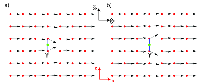
Figure 2: (Color online) Cantings of the spins induced by a single, strong impurity bond with $|J^{\,}_{\mathrm{imp}}|>J^{\,}_{\mathrm{c}}$. The two degenerate ground states correspond to the two solutions $\sigma^{\,}_{\tilde{\boldsymbol{r}}}=+1$ (a) and $\sigma^{\,}_{\tilde{\boldsymbol{r}}}=-1$ (b) of Eq. (29). Red dots indicate sites in the $x$-$z$ plane (red reference frame). The black arrows represent the $\widehat{S}^{x}$ and $\widehat{S}^{y}$ components of the spins (black reference frame). The blue line indicates a frustrating antiferromagnetic bond embedded in the network of ferromagnetic couplings. The green dots indicate the inversion center with respect to which the Hamiltonian is symmetric. The operation of inversion maps the spin configurations (a) and (b) into each other.

III Mapping to an effective Ising Hamiltonian

III.1 Periodic boundary conditions

We are ultimately interested in describing states with a spiralling magnetic order, where the angles of the local magnetization grow linearly with distance. However, before dealing with this possibility, we first analyze a situation anticipating no spiralling. In this case we can impose periodic boundary conditions on the spin angles.

We recall that the set of all directed impurity bonds defines the set $\mathcal{L}\subset\Lambda$ consisting of all the sites $\tilde{\boldsymbol{r}}\in\Lambda$ such that $\langle\tilde{\boldsymbol{r}},\tilde{\boldsymbol{r}}+\boldsymbol{z}\rangle$ is a directed impurity bond. We anticipate that the twist angles across bonds are relatively small, except on the impurity bonds. We therefore make the approximation

$$\begin{split}H^{\,}_{\mathcal{L}}\approx&\,E^{\,}_{\mathrm{FM}}+\frac{1}{2}\sum_{\boldsymbol{r},\boldsymbol{r}^{\prime}\in\Lambda}\theta^{\,}_{\boldsymbol{r}}\,D^{(0)}_{\boldsymbol{r}-\boldsymbol{r}^{\prime}}\,\theta^{\,}_{\boldsymbol{r}^{\prime}}\\ &\,-\sum_{\tilde{\boldsymbol{r}}\in\mathcal{L}}\left[\frac{J^{\,}_{\perp}}{2}\,\left(\Delta\theta^{\,}_{\tilde{\boldsymbol{r}}}\right)^{2}-|J^{\,}_{\mathrm{imp}}|\,\cos\Delta\theta^{\,}_{\tilde{\boldsymbol{r}}}\right],\end{split}$$ (15a)

where $$\Delta\theta^{\,}_{\tilde{\boldsymbol{r}}}$$ is the canting angle across the impurity bond,

$$\Delta\theta^{\,}_{\tilde{\boldsymbol{r}}}\equiv\theta^{\,}_{\tilde{\boldsymbol{r}}}-\theta^{\,}_{\tilde{\boldsymbol{r}}+\boldsymbol{z}}.$$ (15b)

This approximation is certainly valid on the majority of bonds in the limit of a dilute concentration of impurity bonds,

$$n^{\,}_{\mathrm{imp}}\,\raisebox{0.85pt}{.}\raisebox{2.85pt}{.}\!\!=\,\frac{|\mathcal{L}|}{|\Lambda|}\ll 1,$$ (16)

which we will assume from now on.

We are going to establish under what conditions there is a configuration of angles other than the ferromagnetic one that minimize the energy (15a) in the presence of impurity bonds anchored on the set $\mathcal{L}$.

First, we fix all the angles $\theta^{\,}_{\tilde{\boldsymbol{r}}}$ and $\theta^{\,}_{\tilde{\boldsymbol{r}}+\boldsymbol{z}}$ with $\tilde{\boldsymbol{r}}\in\mathcal{L}$ and integrate out the angles on all other sites, i.e., on all sites from $\Lambda\setminus(\mathcal{L}\cup\mathcal{L}+\boldsymbol{z})$. Within our spin wave approximation, and treating the angles as non-compact variables, this can be done exactly (at any temperature where the spin wave approximation is justified) since those angular variables enter the Hamiltonian quadratically. Here, we carry out the calculation at $T=0$ by solving the saddle-point equations for all angles on the sites $\Lambda\setminus(\mathcal{L}\cup\mathcal{L}+\boldsymbol{z})$. In this way, we shall find the angles $\theta^{\,}_{\boldsymbol{r}}$, as well as an effective Hamiltonian, expressed solely in terms of the angles $\{\theta^{\,}_{\tilde{\boldsymbol{r}}},\tilde{\boldsymbol{r}}\in\mathcal{L}\cup\mathcal{L}+\boldsymbol{z}\}$.

The minimization over all $\boldsymbol{r}\in\Lambda\setminus(\mathcal{L}\cup\mathcal{L}+\boldsymbol{z})$ requires

$$\begin{split}\sum_{\boldsymbol{r}^{\prime}\in\Lambda}D^{(0)}_{\boldsymbol{r}-\boldsymbol{r}^{\prime}}\,\theta^{\,}_{\boldsymbol{r}^{\prime}}=&\,0.\end{split}$$ (17a)

We supplement the set (17a) of linear equations by

$$\begin{split}\sum_{\boldsymbol{r}^{\prime}\in\Lambda}D^{(0)}_{\tilde{\boldsymbol{r}}-\boldsymbol{r}^{\prime}}\,\theta^{\,}_{\boldsymbol{r}^{\prime}}=&\,\chi^{\,}_{\tilde{\boldsymbol{r}}},\end{split}$$ (17b)

whereby $\tilde{\boldsymbol{r}}\in\mathcal{L}\cup\mathcal{L}+\boldsymbol{z}$ runs over all sites in $\Lambda$ that are end points of an impurity bond (two sites per impurity bond). Here, $\chi^{\,}_{\tilde{\boldsymbol{r}}}$ has to be chosen in such a way that the saddle-point equations (17) are satisfied as $\theta^{\,}_{\tilde{\boldsymbol{r}}}$ and $\theta^{\,}_{\tilde{\boldsymbol{r}}+\boldsymbol{z}}$ take their prescribed values.

Inverting Eqs. (17a) and (17b) for any $\boldsymbol{r}\in\Lambda$, we obtain

$$\theta^{\,}_{\boldsymbol{r}}=\theta^{\,}_{0}+\sum_{\tilde{\boldsymbol{r}}^{\prime}\in\mathcal{L}\cup\mathcal{L}+\boldsymbol{z}}G^{(0)}_{\boldsymbol{r},\tilde{\boldsymbol{r}}^{\prime}}\,\chi^{\,}_{\tilde{\boldsymbol{r}}^{\prime}},$$ (18)

where $\theta^{\,}_{0}\in[0,2\pi[$ is the angle of the magnetization far away from impurities. Restricting ourselves to the subset $\tilde{\boldsymbol{r}}\in\mathcal{L}\cup\mathcal{L}+\boldsymbol{z}$, Eq. (18) can be inverted to yield

$$\chi^{\,}_{\tilde{\boldsymbol{r}}}=\sum_{\tilde{\boldsymbol{r}}^{\prime}\in\mathcal{L}\cup\mathcal{L}+\boldsymbol{z}}\widetilde{G}^{(0)-1}_{\tilde{\boldsymbol{r}},\tilde{\boldsymbol{r}}^{\prime}}\,\left(\theta^{\,}_{\tilde{\boldsymbol{r}}^{\prime}}-\theta^{\,}_{0}\right),$$ (19)

where $\widetilde{G}^{(0)}$ is the $2|\mathcal{L}|\times 2|\mathcal{L}|$ matrix obtained by restricting $G^{(0)}_{{\boldsymbol{r}},{\boldsymbol{r}}^{\prime}}$ to the sites belonging to the impurity bonds [$\widetilde{G}^{(0)}_{\tilde{{\boldsymbol{r}}},\tilde{{\boldsymbol{r}}}^{\prime}}\equiv G^{(0)}_{\tilde{{\boldsymbol{r}}},\tilde{{\boldsymbol{r}}}^{\prime}}$]. Combining Eqs. (18) and (19), we obtain for any $\boldsymbol{r}\in\Lambda$

$$\theta^{\,}_{\boldsymbol{r}}=\theta^{\,}_{0}+\sum_{\tilde{{\boldsymbol{r}}}^{\prime},\tilde{{\boldsymbol{r}}}^{\prime\prime}\in\mathcal{L}\cup\mathcal{L}+\boldsymbol{z}}G^{(0)}_{\boldsymbol{r},\tilde{{\boldsymbol{r}}}^{\prime}}\,\widetilde{G}^{(0)-1}_{\tilde{{\boldsymbol{r}}}^{\prime},\tilde{{\boldsymbol{r}}}^{\prime\prime}}\,\left(\theta^{\,}_{\tilde{{\boldsymbol{r}}}^{\prime\prime}}-\theta^{\,}_{0}\right).$$ (20)

The algebraic decay of $G^{(0)}_{\boldsymbol{r}}$ ensures that the distortions in the angular pattern also have algebraic tails.

Second, we evaluate the energy (15a) at the saddle point (20). We thereby obtain the effective energy

$$H^{\,}_{\mathrm{eff}}\!\left(\left\{\theta^{\,}_{\tilde{\boldsymbol{r}}},\theta^{\,}_{\tilde{\boldsymbol{r}}+\boldsymbol{z}},\tilde{{\boldsymbol{r}}}\in\mathcal{L}\right\}\right)\,\raisebox{0.85pt}{.}\raisebox{2.85pt}{.}\!\!=\,\frac{1}{2}\sum_{\tilde{{\boldsymbol{r}}},\tilde{{\boldsymbol{r}}}^{\prime}\in\mathcal{L}\cup\mathcal{L}+\boldsymbol{z}}\theta^{\,}_{\tilde{\boldsymbol{r}}}\,\widetilde{G}^{(0)-1}_{\tilde{\boldsymbol{r}},\tilde{\boldsymbol{r}}^{\prime}}\,\theta^{\,}_{\tilde{\boldsymbol{r}}^{\prime}}-\sum_{\tilde{\boldsymbol{r}}\in\mathcal{L}}\left[\frac{J^{\,}_{\perp}}{2}\,\left(\theta^{\,}_{\tilde{\boldsymbol{r}}+\boldsymbol{z}}-\theta^{\,}_{\tilde{\boldsymbol{r}}}\right)^{2}-|J^{\,}_{\mathrm{imp}}|\,\cos\left(\theta^{\,}_{\tilde{\boldsymbol{r}}+\boldsymbol{z}}-\theta^{\,}_{\tilde{\boldsymbol{r}}}\right)\right],$$ (21)

where we have assumed that the magnetization far away from the impurities are oriented along $\theta^{\,}_{0}=0$, making use of the fact that the constant $\theta^{\,}_{0}$ can be chosen freely, since rotating all spins by the same angle does not affect the energy. In what follows, we will drop such additive constants. Note that the derivation of the effective action (21), starting from the Hamiltonian (15a), is exact at any temperature, if we use the Gaussian approximation and treat the domain of the angles $\theta^{\,}_{{\boldsymbol{r}}}$ as non-compact, ignoring that the energy is in fact $2\pi$-periodic in the angles.

For the third and last step we assume $T=0$. We minimize the effective action (21) with respect to the impurity bond angles $\theta^{\,}_{\tilde{\boldsymbol{r}}}$ and $\theta^{\,}_{\tilde{\boldsymbol{r}}+\boldsymbol{z}}$ with $\tilde{\boldsymbol{r}}\in\mathcal{L}$. This can be done exactly for a single impurity bond, and approximately in the case of a dilute set of impurities.

III.1.1 The case of a single impurity bond

In the case of a single impurity bond $\langle\tilde{\boldsymbol{r}},\tilde{\boldsymbol{r}}+\boldsymbol{z}\rangle$ represented by the single site $\mathcal{L}=\{\tilde{\boldsymbol{r}}\}$, the inverse of the $2\times 2$ symmetric matrix with elements $\widetilde{G}^{(0)}_{\tilde{{\boldsymbol{r}}},\tilde{{\boldsymbol{r}}}}$, $\widetilde{G}^{(0)}_{\tilde{{\boldsymbol{r}}},\tilde{{\boldsymbol{r}}}+\boldsymbol{z}}$, $\widetilde{G}^{(0)}_{\tilde{{\boldsymbol{r}}}+\boldsymbol{z},\tilde{{\boldsymbol{r}}}}$, $\widetilde{G}^{(0)}_{\tilde{{\boldsymbol{r}}}+\boldsymbol{z},\tilde{{\boldsymbol{r}}}+\boldsymbol{z}}$, is

$$\widetilde{G}^{(0)-1}_{{{\boldsymbol{r}}},{{\boldsymbol{r}}}^{\prime}}=\frac{G^{(0)}_{\boldsymbol{0}}\,\delta^{\,}_{{{\boldsymbol{r}}},{{\boldsymbol{r}}}^{\prime}}-G^{(0)}_{\boldsymbol{z}}\,\left(\delta^{\,}_{{{\boldsymbol{r}}},{{\boldsymbol{r}}}^{\prime}+\boldsymbol{z}}+\delta^{\,}_{{{\boldsymbol{r}}},{{\boldsymbol{r}}}^{\prime}-\boldsymbol{z}}\right)}{\left(G^{(0)}_{\boldsymbol{0}}\right)^{2}-\left(G^{(0)}_{\boldsymbol{z}}\right)^{2}},$$ (22)

where ${\boldsymbol{r}}$, $\boldsymbol{r}^{\prime}\in\{\tilde{\boldsymbol{r}},\tilde{\boldsymbol{r}}+\boldsymbol{z}\}$.

If we use Eq. (22) in the Hamiltonian (21) we find the effective energy

$$H^{(1)}_{\mathrm{eff}}\left(\theta^{\,}_{\tilde{\boldsymbol{r}}},\theta^{\,}_{\tilde{\boldsymbol{r}}+\boldsymbol{z}}\right)=\frac{1}{4}\,\frac{\left(\theta^{\,}_{\tilde{\boldsymbol{r}}}+\theta^{\,}_{\tilde{\boldsymbol{r}}+\boldsymbol{z}}\right)^{2}}{G^{(0)}_{\boldsymbol{0}}+G^{(0)}_{\boldsymbol{z}}}+\frac{1}{4}\,\frac{\left(\theta^{\,}_{\tilde{\boldsymbol{r}}}-\theta^{\,}_{\tilde{\boldsymbol{r}}+\boldsymbol{z}}\right)^{2}}{G^{(0)}_{\boldsymbol{0}}-G^{(0)}_{\boldsymbol{z}}}-\frac{J^{\,}_{\perp}}{2}\,\left(\theta^{\,}_{\tilde{\boldsymbol{r}}}-\theta^{\,}_{\tilde{\boldsymbol{r}}+\boldsymbol{z}}\right)^{2}+|J^{\,}_{\mathrm{imp}}|\,\cos\left(\theta^{\,}_{\tilde{\boldsymbol{r}}}-\theta^{\,}_{\tilde{\boldsymbol{r}}+\boldsymbol{z}}\right).$$ (23)

The center-of-mass angle $\theta^{\,}_{\tilde{\boldsymbol{r}}}+\theta^{\,}_{\tilde{\boldsymbol{r}}+\boldsymbol{z}}$ and the relative angle $\theta^{\,}_{\tilde{\boldsymbol{r}}}-\theta^{\,}_{\tilde{\boldsymbol{r}}+\boldsymbol{z}}$ are decoupled in $H^{(1)}_{\mathrm{eff}}(\theta^{\,}_{\tilde{\boldsymbol{r}}},\theta^{\,}_{\tilde{\boldsymbol{r}}+\boldsymbol{z}})$. The effective Hamiltonian (23) is invariant under the transformation

$$\theta^{\,}_{\tilde{\boldsymbol{r}}}+\theta^{\,}_{\tilde{\boldsymbol{r}}+\boldsymbol{z}}\mapsto\theta^{\,}_{\tilde{\boldsymbol{r}}}+\theta^{\,}_{\tilde{\boldsymbol{r}}+\boldsymbol{z}},\qquad\theta^{\,}_{\tilde{\boldsymbol{r}}}-\theta^{\,}_{\tilde{\boldsymbol{r}}+\boldsymbol{z}}\mapsto-\left(\theta^{\,}_{\tilde{\boldsymbol{r}}}-\theta^{\,}_{\tilde{\boldsymbol{r}}+\boldsymbol{z}}\right).$$ (24)

This symmetry is inherited from the fact that Hamiltonian (21) is invariant under the inversion symmetry with respect to the bond center $\boldsymbol{R}=\tilde{\boldsymbol{r}}+(\boldsymbol{z}/2)$.

Minimization over $\theta^{\,}_{\tilde{\boldsymbol{r}}}+\theta^{\,}_{\tilde{\boldsymbol{r}}+\boldsymbol{z}}$ imposes the condition that the two angular distortions away from the asymptotic $\theta^{\,}_{0}$ on either side of the impurity bond are opposite,

$$\theta^{\,}_{\tilde{{\boldsymbol{r}}}}=-\theta^{\,}_{\tilde{\boldsymbol{r}}+\boldsymbol{z}}.$$ (25)

The remaining degree of freedom is the canting angle across the impurity bond,

$$\Delta\theta^{\,}_{\tilde{\boldsymbol{r}}}\equiv\theta^{\,}_{\tilde{\boldsymbol{r}}}-\theta^{\,}_{\tilde{\boldsymbol{r}}+\boldsymbol{z}},$$ (26)

with $-\pi<\Delta\theta^{\,}_{\tilde{\boldsymbol{r}}}\leq\pi$, in terms of which the effective restricted (eff/res) Hamiltonian becomes

$$H^{(1)}_{\mathrm{eff/res}}(\Delta\theta^{\,}_{\tilde{\boldsymbol{r}}})\,\raisebox{0.85pt}{.}\raisebox{2.85pt}{.}\!\!=\,\frac{1}{2}\,J^{\,}_{\mathrm{c}}\,\left(\Delta\theta^{\,}_{\tilde{\boldsymbol{r}}}\right)^{2}+|J^{\,}_{\mathrm{imp}}|\,\cos\left(\Delta\theta^{\,}_{\tilde{\boldsymbol{r}}}\right),$$ (27a)

where we have introduced the short-hand notation

$$J^{\,}_{\mathrm{c}}\,\raisebox{0.85pt}{.}\raisebox{2.85pt}{.}\!\!=\,\frac{1}{2\left(G^{(0)}_{\boldsymbol{0}}-G^{(0)}_{\boldsymbol{z}}\right)}-J^{\,}_{\perp}.$$ (27b)

The coupling $J^{\,}_{\mathrm{c}}$ depends parametrically on $J^{\,}_{\parallel}$ and $J^{\,}_{\perp}$. The rationale for the subscript in $J^{\,}_{\mathrm{c}}$ is the following. For small $|J^{\,}_{\mathrm{imp}}|$, i.e., $|J^{\,}_{\mathrm{imp}}|<J^{\,}_{\mathrm{c}}$, $H^{(1)}_{\mathrm{eff/res}}(\Delta\theta^{\,}_{\tilde{\boldsymbol{r}}})$ has a single minimum at

$$\Delta\theta^{\,}_{\tilde{\boldsymbol{r}}}=0.$$ (28)

However, for $|J^{\,}_{\mathrm{imp}}|>J^{\,}_{\mathrm{c}}$, $H^{(1)}_{\mathrm{eff/res}}(\Delta\theta^{\,}_{\tilde{\boldsymbol{r}}})$ develops a double well with two degenerate minima. The two degenerate minima occur at the relative canting angles

$$\Delta\theta^{\,}_{\tilde{\boldsymbol{r}}}=\sigma^{\,}_{\tilde{\boldsymbol{r}}}\,\Delta\theta,$$ (29a)

with $$\sigma^{\,}_{\tilde{\boldsymbol{r}}}=\pm 1 \Delta\theta$$ and being the positive solution of

$$\Delta\theta=\frac{|J^{\,}_{\mathrm{imp}}|}{J^{\,}_{\mathrm{c}}}\sin\Delta\theta.$$ (29b)

When $|J^{\,}_{\mathrm{imp}}|>J^{\,}_{\mathrm{c}}$ and the temperature $T$ is sufficiently small, namely,

$$k^{\,}_{\mathrm{B}}\,T\ll J^{\,}_{\mathrm{c}}-|J^{\,}_{\mathrm{imp}}|\,\cos(\Delta\theta),$$ (30)

thermal fluctuations around the minima of the double well are small. We will thus call $|\Delta\theta^{\,}_{\tilde{\boldsymbol{r}}}|$ a hard degree of freedom, while we refer to the Ising variable $\mathrm{sgn}(\Delta\theta^{\,}_{\tilde{\boldsymbol{r}}})=\sigma^{\,}_{\tilde{\boldsymbol{r}}}$ as a soft degree of freedom. This terminology is motivated by expanding about the minimum of the double potential well, $\sigma^{\,}_{\tilde{\boldsymbol{r}}}\,\Delta\theta$, which is closest to $\Delta\theta^{\,}_{\tilde{\boldsymbol{r}}}$

$$H^{(1)}_{\mathrm{eff/res}}(\Delta\theta^{\,}_{\tilde{\boldsymbol{r}}})-H^{(1)}_{\mathrm{eff/res}}(\Delta\theta)$$ (31)

$$\qquad=\frac{1}{2}\left[J^{\,}_{\mathrm{c}}-|J^{\,}_{\mathrm{imp}}|\,\cos(\Delta\theta)\right]\left({|\Delta\theta^{\,}_{\tilde{\boldsymbol{r}}}|-\Delta\theta}\right)^{2}+\cdots.$$

When the temperature is small compared to the curvature at the two minima, thermal fluctuations of the hard degree of freedom $|\Delta\theta^{\,}_{\tilde{\boldsymbol{r}}}|$ are much smaller than fluctuations due to the soft degree of freedom $\sigma^{\,}_{\tilde{\boldsymbol{r}}}$. We will thus ignore the latter in the range (30) of temperatures.

If we use the values of the relative angle (15b) at the pair of minima (29) in combination with Eqs. (25) and (20) with $\theta^{\,}_{0}=0$, we obtain the two canting patterns shown in Fig. 2.

The combination $2(G^{(0)}_{\boldsymbol{0}}-G^{(0)}_{\boldsymbol{z}})=\Gamma^{(0)}_{\boldsymbol{r}=\boldsymbol{0}}$ entering $J^{\,}_{\mathrm{c}}$ in Eq. (27b) can be expressed with the help of Eq. (13a) as

$$\Gamma^{(0)}_{\boldsymbol{r}=\boldsymbol{0}}=2\left(G^{(0)}_{\boldsymbol{0}}-G^{(0)}_{\boldsymbol{z}}\right)=\frac{1}{J^{\,}_{\mathrm{c}}+J^{\,}_{\perp}}=\frac{1}{|\Lambda|}\sum_{\boldsymbol{k}\in\mathrm{BZ}(\Lambda)\setminus\{\boldsymbol{0}\}}\frac{\left(1-\cos{k^{\,}_{z}}\right)}{J^{\,}_{\parallel}\left(2-\cos k^{\,}_{x}-\cos k^{\,}_{y}\right)+J^{\,}_{\perp}\left(1-\cos k^{\,}_{z}\right)}.$$ (32)

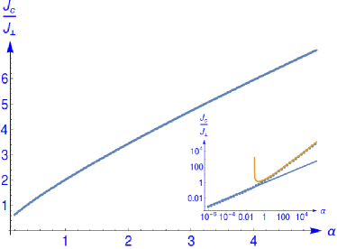
Figure 3: (Color online) Critical impurity bond strength $J^{\,}_{\mathrm{c}}$ (Eq. 27b) (blue dots), as a function of the ratio of couplings $\alpha\equiv J^{\,}_{\parallel}/J^{\,}_{\perp}$. The inset shows the same function on a logarithmic plot. For strong anisotropies, one finds the asymptotics $J^{\,}_{\mathrm{c}}(\alpha\ll 1)/J^{\,}_{\perp}\approx C^{\,}_{1}\sqrt{\alpha}$ (blue line) and $J^{\,}_{\mathrm{c}}(\alpha\gg 1)/J^{\,}_{\perp}\approx 2\pi\alpha/[\ln(\alpha)+C^{\,}_{2}]$ (yellow curve), where $C^{\,}_{1}=\int^{\pi}_{0}\mathrm{d}x\mathrm{d}y\sqrt{\sin^{2}x+\sin^{2}y}/\pi^{2}\approx 0.958$ and $C^{\,}_{2}=(5\ln 2-1)\approx 2.47$.

For isotropic couplings $J^{\,}_{\parallel}=J^{\,}_{\perp}=J$, this evaluates to

$$\Gamma^{(0)}_{\boldsymbol{0}}=\frac{1}{3J},$$ (33)

which yields the critical coupling

$$J^{\,}_{\mathrm{c}}=2J.$$ (34)

For general couplings with ratio

$$\alpha\equiv\frac{J^{\,}_{\parallel}}{J^{\,}_{\perp}},$$ (35)

we plot the threshold value of $J^{\,}_{\mathrm{c}}/J^{\,}_{\perp}$ in Fig. 3 together with asymptotic expressions that become valid in the limit of strong anisotropy.

III.2 The case of a dilute set of impurity bonds

When the density of impurity bonds is finite, we cannot rely on the explicit representation (22). However, at a small impurity concentration, the interaction between the angles on the same impurity bond is much stronger than the coupling between angles on different impurity bonds. It thus makes sense to split $\widetilde{G}^{(0)}$ into a bond-local term [with inverse on every bond given by Eq. (22)] and a bond-off-diagonal term according to

$$\widetilde{G}^{(0)}\equiv\widetilde{G}^{(0)}_{\mathrm{loc}}+\widetilde{G}^{(0)}_{\mathrm{nonloc}},$$ (36)

and to approximate its inverse as

$$\widetilde{G}^{(0)-1}\approx\widetilde{G}^{(0)-1}_{\mathrm{loc}}-\widetilde{G}^{(0)-1}_{\mathrm{loc}}\,\widetilde{G}^{(0)}_{\mathrm{nonloc}}\,\widetilde{G}^{(0)-1}_{\mathrm{loc}}.$$ (37)

This yields the Hamiltonian

$$H^{\,}_{\mathrm{eff}}\left(\left\{\theta^{\,}_{\tilde{\boldsymbol{r}}},\theta^{\,}_{\tilde{\boldsymbol{r}}+\boldsymbol{z}},\tilde{{\boldsymbol{r}}}\in\mathcal{L}\right\}\right)\approx\sum_{\tilde{\boldsymbol{r}}\in\mathcal{L}}H^{(1)}_{\mathrm{eff}}(\theta^{\,}_{\tilde{\boldsymbol{r}}},\theta^{\,}_{\tilde{\boldsymbol{r}}+\boldsymbol{z}})-\frac{1}{2}\sum_{\tilde{{\boldsymbol{r}}},\tilde{{\boldsymbol{r}}}^{\prime}\in\mathcal{L}\cup\mathcal{L}+\boldsymbol{z}}\theta^{\,}_{\tilde{\boldsymbol{r}}}\,\left[\widetilde{G}^{(0)-1}_{\mathrm{loc}}\,\widetilde{G}^{(0)}_{\mathrm{nonloc}}\,\widetilde{G}^{(0)-1}_{\mathrm{loc}}\right]^{\,}_{\tilde{\boldsymbol{r}},\tilde{\boldsymbol{r}}^{\prime}}\,\theta^{\,}_{\tilde{\boldsymbol{r}}^{\prime}},$$ (38a)

where $H^{(1)}_{\mathrm{eff}}(\theta^{\,}_{\tilde{\boldsymbol{r}}},\theta^{\,}_{\tilde{\boldsymbol{r}}+\boldsymbol{z}})$ is given by Eq. (23).

Since this term is dominant at low impurity concentration, it is again reasonable to restrict the angular configurations to the subspace given by

$$\theta^{\,}_{\tilde{{\boldsymbol{r}}}}=-\theta^{\,}_{\tilde{\boldsymbol{r}}+\boldsymbol{z}}=\frac{\Delta\theta^{\,}_{\tilde{\boldsymbol{r}}}}{2}\Longrightarrow\theta^{\,}_{\tilde{{\boldsymbol{r}}}}+\theta^{\,}_{\tilde{\boldsymbol{r}}+\boldsymbol{z}}=0,\qquad\theta^{\,}_{\tilde{{\boldsymbol{r}}}}-\theta^{\,}_{\tilde{\boldsymbol{r}}+\boldsymbol{z}}=\Delta\theta^{\,}_{\tilde{\boldsymbol{r}}},$$ (39)

as in the single impurity-bond problem of Eq. (23). This leads to the effective restricted Hamiltonian [compare with Eq. (27)]

$$H^{\,}_{\mathrm{eff/res}}\!\left(\left\{\Delta\theta^{\,}_{\tilde{\boldsymbol{r}}}\right\}\right)\,\raisebox{0.85pt}{.}\raisebox{2.85pt}{.}\!\!=\, \,\sum_{\tilde{\boldsymbol{r}}\in\mathcal{L}}H^{(1)}_{{\mathrm{eff/res}}}\left(\Delta\theta^{\,}_{\tilde{\boldsymbol{r}}}\right)-\frac{1}{2}\sum_{\tilde{\boldsymbol{r}}\neq\tilde{\boldsymbol{r}}^{\prime}\in\mathcal{L}}\frac{\Delta\theta^{\,}_{\tilde{\boldsymbol{r}}}}{2\left(G^{(0)}_{\boldsymbol{0}}-G^{(0)}_{\boldsymbol{z}}\right)}\,\left(2G^{\,}_{\tilde{\boldsymbol{r}},\tilde{\boldsymbol{r}}^{\prime}}-{G}^{\,}_{\tilde{\boldsymbol{r}}+\boldsymbol{z},\tilde{\boldsymbol{r}}^{\prime}}-{G}^{\,}_{\tilde{\boldsymbol{r}},\tilde{\boldsymbol{r}}^{\prime}+\boldsymbol{z}}\right)\,\frac{\Delta\theta^{\,}_{\tilde{\boldsymbol{r}}^{\prime}}}{2\left(G^{(0)}_{\boldsymbol{0}}-G^{(0)}_{\boldsymbol{z}}\right)}$$

$$= \,\sum_{\tilde{\boldsymbol{r}}\in\mathcal{L}}H^{(1)}_{{\mathrm{eff/res}}}(\Delta\theta^{\,}_{\tilde{\boldsymbol{r}}})-\frac{1}{2\left(\Gamma^{(0)}_{\boldsymbol{0}}\right)^{2}}\sum_{\tilde{\boldsymbol{r}}\neq\tilde{\boldsymbol{r}}^{\prime}\in\mathcal{L}}\Delta\theta^{\,}_{\tilde{\boldsymbol{r}}}\,\Gamma^{(0)}_{\tilde{\boldsymbol{r}}-\tilde{\boldsymbol{r}}^{\prime}}\,\Delta\theta^{\,}_{\tilde{\boldsymbol{r}}^{\prime}},$$ (40)

where the interaction $\Gamma^{(0)}_{\tilde{\boldsymbol{r}}-\tilde{\boldsymbol{r}}^{\prime}}$ is seen to be mediated by the combination of Green’s functions introduced in Eq. (13a) that scales like an anti-dipolar interaction at long distances.

As it should be, the effective Hamiltonian is invariant under both the global rotation $\theta^{\,}_{\tilde{\boldsymbol{r}}}\mapsto\theta^{\,}_{\tilde{\boldsymbol{r}}}+\Theta$, $\Theta\in[0,2\pi[$ and the global Ising symmetry $\theta^{\,}_{\tilde{\boldsymbol{r}}}\mapsto-\theta^{\,}_{\tilde{\boldsymbol{r}}}$ for all $\tilde{\boldsymbol{r}}\in\mathcal{L}$.

It remains to minimize $H^{\,}_{\mathrm{eff/res}}{\left(\left\{\Delta\theta^{\,}_{\tilde{\boldsymbol{r}}}\right\}\right)}$ with respect to the canting angles $\Delta\theta^{\,}_{\tilde{\boldsymbol{r}}}$ on the impurity bonds. The corresponding saddle point equation reads,

$$\Delta\theta^{\,}_{\tilde{\boldsymbol{r}}}=\frac{|J^{\,}_{\mathrm{imp}}|}{J^{\,}_{\mathrm{c}}}\sin\Delta\theta^{\,}_{\tilde{\boldsymbol{r}}}+\Xi^{\,}_{\tilde{\boldsymbol{r}}},$$ (41a)

where

$$\Xi^{\,}_{\tilde{\boldsymbol{r}}}\,\raisebox{0.85pt}{.}\raisebox{2.85pt}{.}\!\!=\,\frac{1}{J^{\,}_{\mathrm{c}}}\sum_{\tilde{\boldsymbol{r}}^{\prime}\in\mathcal{L}\setminus\{\tilde{\boldsymbol{r}}\}}\frac{\Gamma^{(0)}_{\tilde{\boldsymbol{r}}-\tilde{\boldsymbol{r}}^{\prime}}}{\left(\Gamma^{(0)}_{\boldsymbol{0}}\right)^{2}}\,\Delta\theta^{\,}_{\tilde{\boldsymbol{r}}^{\prime}}.$$ (41b)

As before, the ferromagnetic state (28) is a solution of Eqs. (41a) and (41b), but it becomes unstable for sufficiently large $|J^{\,}_{\mathrm{imp}}|$.

The term $\Xi^{\,}_{\tilde{\boldsymbol{r}}}$ is expected to be dominated by the closest neighbor bonds, since the sum is over a set of decreasing terms, which, for a valid saddle point, contribute with alternating signs. Using Eqs. (14) and (41b), one expects that $\Xi^{\,}_{\tilde{\boldsymbol{r}}}$ scales as $n^{\,}_{\mathrm{imp}}$. In that case, the condition

$$\frac{|J^{\,}_{\mathrm{imp}}|}{J^{\,}_{\mathrm{c}}}\gg\Xi^{\,}_{\tilde{\boldsymbol{r}}}$$ (42)

will be met for sufficiently large values of $J_{\mathrm{imp}}$ and sufficiently small values of $n^{\,}_{\mathrm{imp}}$. Under the condition (42), local minima of the Hamiltonian (15a), i.e., solutions to Eq. (41), exist, which locally look like the solution for a single antiferromagnetic impurity bond.

In the dilute impurity regime, a low energy state will have a canting of angles across the impurities bonds close to the single impurity case, i.e.,

$$\Delta\theta^{\,}_{\tilde{\boldsymbol{r}}}\approx\sigma^{\,}_{\tilde{\boldsymbol{r}}}\,\Delta\theta.$$ (43a)

Inserting this Ansatz into the effective Hamiltonian (40), we obtain the effective Ising model

$$\begin{split}H^{\,}_{\mathcal{L}}[\sigma^{\,}_{\tilde{\boldsymbol{r}}}]\,\raisebox{0.85pt}{.}\raisebox{2.85pt}{.}\!\!=\,&\,E^{\,}_{\mathrm{FM}}+E(\Delta\theta)\,|\mathcal{L}|\\ &\,-\frac{1}{2}\,\left(\frac{\Delta\theta}{\Gamma_{\boldsymbol{0}}^{(0)}}\right)^{2}\sum_{\tilde{\boldsymbol{r}}\neq\tilde{\boldsymbol{r}}^{\prime}\in\mathcal{L}}\sigma^{\,}_{\tilde{\boldsymbol{r}}}\,\Gamma^{(0)}_{\tilde{\boldsymbol{r}}-\tilde{\boldsymbol{r}}^{\prime}}\,\sigma^{\,}_{\tilde{\boldsymbol{r}}^{\prime}}.\end{split}$$ (43b)

This effective Ising model is invariant under the global Ising symmetry $\sigma^{\,}_{\tilde{\boldsymbol{r}}}\mapsto-\sigma^{\,}_{\tilde{\boldsymbol{r}}}$ for all $\tilde{\boldsymbol{r}}\in\mathcal{L}$. Equation (43b) is the main result of Sec. III.2.

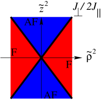
Figure 4: (Color online) Sign of the (anti-)dipolar interaction $\Gamma^{(0)}_{\tilde{\boldsymbol{r}}}$ (14) between cantings, in the $\tilde{\rho}^{2}-\tilde{z}^{2}$-plane (with $\tilde{\rho}^{2}\equiv\tilde{x}^{2}+\tilde{y}^{2}$). Along the $z$-axis the interactions are antiferromagnetic, while for separation along the $xy-$plane they are ferromagnetic. The sign change occurs on the cone described by $J^{\,}_{\perp}\tilde{\rho}^{2}=2J^{\,}_{\parallel}\tilde{z}^{2}$. In the quasi-one-dimensional limit $J^{\,}_{\parallel}/J^{\,}_{\perp}\to 0$, the interaction $\Gamma^{(0)}_{\tilde{\boldsymbol{r}}}$ is ferromagnetic for any $\tilde{\rho}^{2}>0$. In the quasi-two-dimensional limit $J^{\,}_{\perp}/J^{\,}_{\parallel}\to 0$, $\Gamma^{(0)}_{\tilde{\boldsymbol{r}}}$ is antiferromagnetic for any $\tilde{z}^{2}>0$.

The interaction $\Gamma^{(0)}_{\tilde{\boldsymbol{r}}}$ between a pair of Ising variables a distance $\tilde{\boldsymbol{r}}$ apart that enters on the right-hand side of Eq. (43b) was derived in Eq. (14). Its asymptotic behavior is that of Ising dipoles ($\sigma^{\,}_{\tilde{\boldsymbol{r}}}$ oriented along the direction $\boldsymbol{z}$), albeit with the opposite sign as compared to the usual dipolar interaction. In the dilute impurity limit, the sign of the two-body interaction $\Gamma^{(0)}_{\boldsymbol{r}}$ depends on the relative position $\tilde{\boldsymbol{r}}$ (see Fig. 4). It is ferromagnetic when

$$\tilde{x}^{2}+\tilde{y}^{2}>\frac{2J^{\,}_{\parallel}}{J^{\,}_{\perp}}\,\tilde{z}^{2},$$ (44a)

vanishing on the conical surface

$$\tilde{x}^{2}+\tilde{y}^{2}=\frac{2J^{\,}_{\parallel}}{J^{\,}_{\perp}}\,\tilde{z}^{2},$$ (44b)

and antiferromagnetic when

$$\tilde{x}^{2}+\tilde{y}^{2}<\frac{2J^{\,}_{\parallel}}{J^{\,}_{\perp}}\,\tilde{z}^{2}.$$ (44c)

III.3 Boundary conditions along the $\boldsymbol{z}$ axis

So far, we have considered the ferromagnetic state, $\theta^{\,}_{\boldsymbol{r}}=0$ for all $\boldsymbol{r}\in\Lambda$, of $H^{\,}_{0}$ defined in Eq. (4) and performed a spin-wave expansion about it, imposing periodic boundary conditions. However, this precludes the possibility that the reference state for the spin wave expansion is non-collinear, and moreover, the periodic boundary conditions on the angles $\theta^{\,}_{\boldsymbol{r}}$ preclude a spiral state. To overcome these limitations, we allow for a linear growth of

$$\theta^{\,}_{\boldsymbol{r}}=\phi^{\,}_{\boldsymbol{r}}+Q\,(\boldsymbol{r}\cdot\boldsymbol{z}),$$ (45)

along the $\boldsymbol{z}$ direction. Here, the global degree of freedom $Q\in[-\pi,\pi[$ describes a constant twist rate, while the local degrees of freedom $\phi^{\,}_{\boldsymbol{r}}$ obey periodic boundary conditions. In finite systems, the twist rate $Q$ along the $\boldsymbol{z}$ direction should be an integer multiple of $2\pi/L^{\,}_{z}$ if we impose periodic boundary conditions on the original spins $\widehat{\boldsymbol{S}}^{\,}_{\boldsymbol{r}}=\cos\theta^{\,}_{\boldsymbol{r}}\,\widehat{\boldsymbol{x}}+\sin\theta^{\,}_{\boldsymbol{r}}\,\widehat{\boldsymbol{y}}$, but this discrete constraint is irrelevant in the thermodynamic limit. With the change of variables (45), the spin-wave approximation (15a) becomes

$$\begin{split}H^{\,}_{\mathcal{L}}\approx&\,E^{\,}_{\mathrm{FM}}+\frac{1}{2}\sum_{\boldsymbol{r},\boldsymbol{r}^{\prime}\in\Lambda}\phi^{\,}_{\boldsymbol{r}}\,D^{(0)}_{\boldsymbol{r}-\boldsymbol{r}^{\prime}}\,\phi^{\,}_{\boldsymbol{r}^{\prime}}+\frac{J^{\,}_{\perp}\,Q^{2}}{2}\,|\Lambda|\\ &\,-\sum_{\tilde{\boldsymbol{r}}\in\mathcal{L}}\left(\frac{J^{\,}_{\perp}}{2}(\Delta\phi^{\,}_{\tilde{\boldsymbol{r}}}-Q)^{2}-|J^{\,}_{\mathrm{imp}}|\cos(\Delta\phi^{\,}_{\tilde{\boldsymbol{r}}}-Q)\right),\end{split}$$ (46a)

where we recall that $$|\Lambda| \Lambda$$ is the number of sites in the host cubic lattice , and we again denote by

$$\Delta\phi^{\,}_{\tilde{\boldsymbol{r}}}\,\raisebox{0.85pt}{.}\raisebox{2.85pt}{.}\!\!=\,\phi^{\,}_{\tilde{\boldsymbol{r}}}-\phi^{\,}_{\tilde{\boldsymbol{r}}+z}$$ (46b)

the twist of $\phi$ across the impurity bond labelled by $\tilde{\boldsymbol{r}}$.

For a low impurity concentration $0<n^{\,}_{\mathrm{imp}}\ll 1$, we assume and will verify a posteriori, that

$$|Q|\sim n^{\,}_{\mathrm{imp}}\ll\Delta\theta,$$ (47)

where $\Delta\theta{\geq 0}$ is the modulus of the canting angle across an isolated impurity bond. The leading effect of the emerging spiral order will appear at order $\mathcal{O}(n^{2}_{\mathrm{imp}})$ in the energy per spin. We therefore expand the impurity bond terms in Eq. (46a), i.e., the second line on the right-hand side of Eq. (46a), up to linear order in $Q$. In this approximation, the saddle-point values for $\Delta\phi^{\,}_{\tilde{\boldsymbol{r}}}$ are therefore again given by

$$\Delta\phi^{\,}_{\tilde{\boldsymbol{r}}}\approx\sigma^{\,}_{\tilde{\boldsymbol{r}}}\,\Delta\theta$$ (48)

up to corrections of order $\mathcal{O}(Q)$. We can neglect those since they lead to corrections to the energy per spin of order $\mathcal{O}(n^{3}_{\mathrm{imp}})$. The angles of spins that do not belong to impurity bonds are again given by Eq. (41), with $\Delta\phi^{\,}_{\tilde{\boldsymbol{r}}}$ replacing $\Delta\theta^{\,}_{\tilde{\boldsymbol{r}}}$. However, minimizing over the twist rate $Q$ after linearization with respect to $Q$ of the second line on the right-hand side of Eq. (46a), yields the non-trivial saddle point value

$$Q= \,-\frac{1}{|\Lambda|}\sum_{\tilde{\boldsymbol{r}}\in\mathcal{L}}\left(\frac{|J^{\,}_{\mathrm{imp}}|}{J^{\,}_{\perp}}\,\sin\left(\Delta\phi^{\,}_{\tilde{\boldsymbol{r}}}\right)+\Delta\phi^{\,}_{\tilde{\boldsymbol{r}}}\right)$$

$$= \,-\Delta\theta\,\frac{J^{\,}_{\mathrm{c}}+J^{\,}_{\perp}}{J^{\,}_{\perp}}\,\frac{1}{|\Lambda|}\sum_{\tilde{\boldsymbol{r}}\in\mathcal{L}}\sigma^{\,}_{\tilde{\boldsymbol{r}}},$$ (49)

where we have used the saddle point equation (29) to reach the second equality. A spontaneous net winding ($Q\neq 0$) of the spins along the $\boldsymbol{z}$ direction thus occurs for canting configurations $\{\sigma^{\,}_{\tilde{\boldsymbol{r}}}\}$ with a net bias. An Ising configuration $\{\sigma^{\,}_{\tilde{\boldsymbol{r}}}\}$ with a net uniform magnetization thus corresponds to a spiral state for the $XY$ spins. Note that the wave vector $Q$ of the spiral is proportional to the magnetization density of the Ising variables.

We can now verify a posteriori the validity of the assumption (47). The maximal value of $|Q|$ is given by

$$|Q|^{\,}_{\mathrm{max}}= \,n^{\,}_{\mathrm{imp}}\,\frac{J^{\,}_{\mathrm{c}}+J^{\,}_{\perp}}{J^{\,}_{\perp}}\,\Delta\theta.$$ (50)

Thus, for

$$n^{\,}_{\mathrm{imp}}\,\ll\frac{J^{\,}_{\perp}}{J^{\,}_{\mathrm{c}}+J^{\,}_{\perp}},$$ (51)

our assumption is certainly self-consistent. In the opposite regime, as $n^{\,}_{\mathrm{imp}}$ approaches 1 from below, the interaction between the planes starts to be dominated by the impurity bonds, which may induce an entirely different ground state with no spiral order.

Injecting the saddle point value of $Q$, Eq. (49), into Eq. (46) and expressing the energy as a function of the Ising variables $\sigma^{\,}_{\tilde{\boldsymbol{r}}}$ leads to the same effective Hamiltonian as in Eq. (43b), except for an additional term $-\frac{J^{\,}_{\perp}\,Q^{2}}{2}\,|\Lambda|$, which expresses the lowering of the total energy due to the coupling of the canting pattern to the spiral order,

$$H^{\,}_{\mathcal{L}}[\sigma^{\,}_{\tilde{\boldsymbol{r}}}]\,\raisebox{0.85pt}{.}\raisebox{2.85pt}{.}\!\!=\, \,E^{\,}_{\mathrm{FM}}+E(\Delta\theta)\,|\mathcal{L}|$$

$$\,-\frac{\gamma}{2}\sum_{\tilde{\boldsymbol{r}}\neq\tilde{\boldsymbol{r}}^{\prime}\in\mathcal{L}}\sigma^{\,}_{\tilde{\boldsymbol{r}}}\,\Gamma^{(0)}_{\tilde{\boldsymbol{r}}-\tilde{\boldsymbol{r}}^{\prime}}\,\sigma^{\,}_{\tilde{\boldsymbol{r}}^{\prime}}-\frac{J^{\,}_{\perp}\,Q^{2}}{2}\,|\Lambda|$$

$$= \,E^{\,}_{\mathrm{FM}}+E(\Delta\theta)\,|\mathcal{L}|$$

$$\,-\frac{1}{2}\sum_{\tilde{\boldsymbol{r}}\neq\tilde{\boldsymbol{r}}^{\prime}\in\mathcal{L}}\sigma^{\,}_{\tilde{\boldsymbol{r}}}\,J^{(\mathrm{I})}_{\tilde{\boldsymbol{r}}-\tilde{\boldsymbol{r}}^{\prime}}\,\sigma^{\,}_{\tilde{\boldsymbol{r}}^{\prime}}-\frac{\gamma\,n^{\,}_{\mathrm{imp}}}{2J^{\,}_{\perp}},$$ (52a)

where we have introduced the constant

$$\gamma\,\raisebox{0.85pt}{.}\raisebox{2.85pt}{.}\!\!=\,\left(\Delta\theta\right)^{2}\,\left(J^{\,}_{\mathrm{c}}+J^{\,}_{\perp}\right)^{2}=\left(\frac{\Delta\theta}{\Gamma_{\boldsymbol{0}}^{(0)}}\right)^{2},$$ (52b)

and the effective Ising interaction

$$\begin{split}J^{(\mathrm{I})}_{\tilde{\boldsymbol{r}}-\tilde{\boldsymbol{r}}^{\prime}}\,\raisebox{0.85pt}{.}\raisebox{2.85pt}{.}\!\!=\,&\,\gamma\,\left(\Gamma^{(0)}_{\tilde{\boldsymbol{r}}-\tilde{\boldsymbol{r}}^{\prime}}\,+\frac{1}{J^{\,}_{\perp}\,|\Lambda|}\right).\end{split}$$ (52c)

Note that the last term in (52a) is non-extensive and thus irrelevant in the thermodynamic limit.

There are two additive contributions to the Ising exchange coupling $J^{(\mathrm{I})}_{\tilde{\boldsymbol{r}}-\tilde{\boldsymbol{r}}^{\prime}}$. The contribution $\Gamma^{(0)}_{\tilde{\boldsymbol{r}}-\tilde{\boldsymbol{r}}^{\prime}}$ represents an (anti)-dipolar two-body interaction between the effective Ising degrees of freedom $\sigma^{\,}_{\tilde{\boldsymbol{r}}}$ associated with the dilute antiferromagnetic bonds. This interaction is long ranged and frustrated, owing to the indefinite sign of the kernel $\Gamma^{(0)}_{\tilde{\boldsymbol{r}}-\tilde{\boldsymbol{r}}^{\prime}}$. The coupling of the canting pattern to the spiral order instead favors a net (ferromagnetic) bias of the cantings $\sigma^{\,}_{\tilde{\boldsymbol{r}}}$ and contributes an all-to-all interaction of strength $\frac{1}{J^{\,}_{\perp}\,|\Lambda|}$, proportional to the inverse volume.

According to the saddle-point equation (41a), a uniform magnetization of the Ising spins $\sigma^{\,}_{\tilde{\boldsymbol{r}}}$ favors a spiral state with a nonvanishing $Q$ for the original $O(2)$ spin degrees of freedom. Hence, if the ground state of Eq. (52) supports a non-vanishing magnetization $\sigma^{\,}_{\tilde{\boldsymbol{r}}}$, the frustration induced by the dilute impurity bonds turns the pristine ferromagnetic order of the impurity-free ground state into spiral order. If instead the ground state supports no net bias of the Ising spins $\sigma^{\,}_{\tilde{\boldsymbol{r}}}$, a state with $Q=0$ is favored, and thus no net winding of the $O(2)$ spins is induced. An example of a possible resulting ground state is a fan-like magnetic state where the Ising spins order in a layered antiferromagnetic pattern. This translates into a pattern of the original $O(2)$ spins ordering essentially ferromagnetically, but with orientations that alternate slightly between successive layers.

The Ising Hamiltonian with anti-dipolar coupling (52) is structurally very similar to Ising systems with standard dipolar couplings, as are realized, e.g., in rare earth compounds with strongly localized magnetic moments, such as LiHo_xY_1-xF₄ at moderate to low dilution $x$  Babkevich et al. (2016). It has been theoretically and experimentally well established that such random dipolar Ising systems exhibit a glass transition towards an amorphous magnetic order at low temperature Alonso and Fernández (2010); Alonso (2015). It may thus come as a surprise that in our case we will find that a change of sign of the dipolar term, in conjunction with the additional term arising from the coupling to the spiral, suffices to induce ferromagnetic Ising order, in spite of the positional randomness of the Ising spins. This difference is presumably largely due to the additional mean-field like interaction mediated by the formation of the spiral, which stabilizes the ferromagnetic phase. That type of interaction is absent in systems of elementary magnetic dipoles, which therefore fall much more easily into a glassy phase.

IV Superlattices of impurity bonds

As Eq. (52) involves long-range two-body interactions whose sign depends on the relative positions of the impurity bonds, the ground state cannot be found explicitly for an arbitrary choice of $\mathcal{L}$, so that in general one has to resort to numerical methods, or to approximate treatments.

However, if the set of impurity bonds $\mathcal{L}$ realizes certain Bravais superlattices, it is possible to establish a sufficient condition for the ground state of the effective Ising Hamiltonian (52) to be ferromagnetic and, thus, for the ground-state spin configuration of the Hamiltonian (15a) to sustain spiral order.

IV.1 Analytical considerations

We consider the case when the subset $\mathcal{L}$ of the cubic host lattice $\Lambda$ forms a Bravais lattice with the basis vectors $\boldsymbol{A}$, $\boldsymbol{B}$, and $\boldsymbol{C}$ given by three independent linear combinations with integer-valued coefficients of $\boldsymbol{a}\equiv(1,0,0)^{\mathsf{T}}$, $\boldsymbol{b}\equiv(0,1,0)^{\mathsf{T}}$, and $\boldsymbol{c}\equiv(0,0,1)^{\mathsf{T}}$. The concentration of the impurity bonds is

$$n^{\,}_{\mathrm{imp}}\equiv\frac{1}{|\boldsymbol{A}\cdot(\boldsymbol{B}\wedge\boldsymbol{C})|}.$$ (53)

In reciprocal space, the superlattice $\mathcal{L}$ defines a small first Brillouin zone $\mathrm{BZ}(\mathcal{L})$, which is $1/n^{\,}_{\mathrm{imp}}$ times smaller than the first Brillouin zone $\mathrm{BZ}(\Lambda)$ of the cubic host lattice $\Lambda$.

For the $|\mathcal{L}|$ Ising degrees of freedom $\sigma^{\,}_{\tilde{\boldsymbol{r}}}$ associated with impurity bonds anchored at $\tilde{\boldsymbol{r}}\in\mathcal{L}$, we use the Fourier representation

$$\sigma^{\,}_{\tilde{\boldsymbol{r}}}=\frac{1}{|\mathcal{L}|}\sum_{\boldsymbol{q}\in\mathrm{BZ}(\mathcal{L})}e^{\mathrm{i}\boldsymbol{q}\cdot\tilde{\boldsymbol{r}}}\,\sigma^{\,}_{\boldsymbol{q}},$$ (54)

where $\mathrm{BZ}(\mathcal{L})$ is the first Brillouin zone associated with the lattice $\mathcal{L}$. For any $\boldsymbol{p}\in\mathbb{R}^{3}$, we shall make use of the identity

$$\frac{1}{|\mathcal{L}|}\sum_{\tilde{\boldsymbol{r}}\in\mathcal{L}}e^{\mathrm{i}\boldsymbol{p}\cdot\tilde{\boldsymbol{r}}}=\sum_{\boldsymbol{\mathsf{G}}\in\mathcal{L}^{\star}}\delta^{\,}_{\boldsymbol{p},\boldsymbol{\mathsf{G}}},$$ (55)

where $\mathcal{L}^{\star}$ denotes the reciprocal lattice of $\mathcal{L}$. The effective Ising Hamiltonian (52) can now be written in reciprocal space as

$$H^{\,}_{\mathcal{L}}= \,E^{\,}_{\mathrm{FM}}\!+\!E({\Delta\theta})\,|\mathcal{L}|$$

$$\,+\frac{\gamma}{2|\mathcal{L}|}\sum_{\boldsymbol{q}\in\mathrm{BZ}(\mathcal{L})}\Upsilon^{\,}_{\boldsymbol{q}}\,\sigma^{\,}_{+\boldsymbol{q}}\,\sigma^{\,}_{-\boldsymbol{q}},$$ (56a)

where $$\gamma$$ is defined by Eq. (52b) and

$$\Upsilon^{\,}_{\boldsymbol{q}}\,\raisebox{0.85pt}{.}\raisebox{2.85pt}{.}\!\!=\,-\sum_{\tilde{\boldsymbol{r}}\in\mathcal{L}\setminus\{\boldsymbol{0}\}}e^{-\mathrm{i}\boldsymbol{q}\cdot\tilde{\boldsymbol{r}}}\,\Gamma^{(0)}_{\tilde{\boldsymbol{r}}}-\frac{n^{\,}_{\mathrm{imp}}}{J^{\,}_{\perp}}\,\delta^{\,}_{\boldsymbol{q},\boldsymbol{0}}.$$ (56b)

Using Eq. (55), we obtain

$$\Upsilon^{\,}_{\boldsymbol{q}}=-n^{\,}_{\mathrm{imp}}\!\sum_{\begin{subarray}{c}\boldsymbol{\mathsf{G}}\in\mathcal{L}^{\star}\\ \boldsymbol{q}+\boldsymbol{\mathsf{G}}\in\mathrm{BZ}(\Lambda)\end{subarray}}\!\Gamma^{(0)}_{\boldsymbol{q}+\boldsymbol{\mathsf{G}}}+\Gamma^{(0)}_{\tilde{\boldsymbol{r}}=\boldsymbol{0}}-\frac{n^{\,}_{\mathrm{imp}}}{J^{\,}_{\perp}}\delta^{\,}_{\boldsymbol{q},\boldsymbol{0}}.$$ (56c)

For a generic choice of the Bravais lattice $\mathcal{L}$ and of the couplings $J^{\,}_{\perp}$, $J^{\,}_{\parallel}$, and $J^{\,}_{\mathrm{imp}}$, the ground state of the Ising Hamiltonian (56) cannot be found in closed form. However, an analytical solution is available in certain cases. For instance, if over the reduced Brillouin zone $\mathrm{BZ}(\mathcal{L})$, the kernel $\Upsilon^{\,}_{\boldsymbol{q}}$ assumes its global minimum at a unique momentum $\boldsymbol{q}^{\,}_{\mathrm{min}}$, such that for all $\tilde{\boldsymbol{r}}\in\mathcal{L}$

$$\sigma^{\mathrm{min}}_{\tilde{\boldsymbol{r}}}=e^{\mathrm{i}\boldsymbol{q}^{\,}_{\mathrm{min}}\cdot\tilde{\boldsymbol{r}}}=\pm 1,$$ (57)

the ground state of the Ising Hamiltonian is then given by the configuration described by Eq. (57). Inserting Eq. (57) into Eqs. (45), (48), and (49), and using the Fourier representation (13a,LABEL:eq:_def_Gammas_and_hat_Gammas_b), one finds

$$\theta^{\mathrm{min}}_{\boldsymbol{r}}=\phi^{\mathrm{min}}_{\boldsymbol{r}}+Q^{\mathrm{min}}\,(\boldsymbol{r}\cdot\boldsymbol{z}),$$ (58a)

where

$$\phi^{\mathrm{min}}_{\boldsymbol{r}}\,\raisebox{0.85pt}{.}\raisebox{2.85pt}{.}\!\!=\,{n^{\,}_{\mathrm{imp}}\sqrt{\gamma}\sum_{\left\{\boldsymbol{k}\in\mathrm{BZ}(\Lambda)|\boldsymbol{k}-\boldsymbol{q}^{\,}_{\mathrm{min}}\in\mathcal{L}^{\star}\setminus\{\boldsymbol{0}\}\right\}}\frac{\left(1-e^{-\mathrm{i}k^{\,}_{z}}\right)\,e^{\mathrm{i}\boldsymbol{k}\cdot\boldsymbol{r}}}{2J^{\,}_{\parallel}\left(2-\cos k^{\,}_{x}-\cos k^{\,}_{y}\right)+2J^{\,}_{\perp}\left(1-\cos k^{\,}_{z}\right)},}$$ (58b)

with $$\gamma$$ defined by Eq. (52b) and

$$Q^{\mathrm{min}}\,\raisebox{0.85pt}{.}\raisebox{2.85pt}{.}\!\!=\,-\frac{\sqrt{\gamma}}{J^{\,}_{\perp}}\,n^{\,}_{\mathrm{imp}}\,\delta^{\,}_{\boldsymbol{q}^{\,}_{\mathrm{min}},\boldsymbol{0}}.$$ (58c)

Examples of $\boldsymbol{q}^{\,}_{\mathrm{min}}$ for which Eq. (57) holds are

$$\boldsymbol{q}^{\,}_{\mathrm{min}}=\boldsymbol{0},$$ (59a)

and

$$\boldsymbol{q}^{\,}_{\mathrm{min}}\in\left\{\pm\frac{1}{2}\,\boldsymbol{A}^{\star},\pm\frac{1}{2}\,\boldsymbol{B}^{\star},\pm\frac{1}{2}\,\boldsymbol{C}^{\star}\right\},$$ (59b)

where $\boldsymbol{A}^{\star}$, $\boldsymbol{B}^{\star}$, and $\boldsymbol{C}^{\star}$ are the basis vectors of the reciprocal lattice $\mathcal{L}^{\star}$. In the former case (59a), $Q^{\mathrm{min}}\neq 0$ and the ground state is an $O(2)$ magnetic spiral, while in the latter case (59b), $Q^{\mathrm{min}}=0$ and thus there is no spiral.

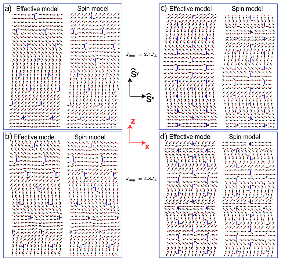
Figure 5: (Color online) Spin configurations of the ground state in an $x$-$z$ plane of the cubic host lattice $\Lambda$. Black arrows represent the $O(2)$ ($XY$) spins defined in Eq. (3) (black reference frame). Red dots represent the sites in a cross section of the cubic host lattice $\Lambda$ (red reference frame). Blue lines represent the impurity bonds. Results are obtained for $J^{\,}_{\parallel}/J^{\,}_{\perp}=1$. Panels (a) and (b) show the comparison between approximate analytical results (as described in Sec. IV.1) and MC simulations of Eq. (60), respectively, for a superlattice with the basis $\boldsymbol{A}=(5,3,2)^{\mathsf{T}}$, $\boldsymbol{B}=(3,4,4)^{\mathsf{T}}$, and $\boldsymbol{C}=(4,5,2)^{\mathsf{T}}$. The superlattice in panels (c) and (d) has the basis $\boldsymbol{A}=(3,3,2)^{\mathsf{T}}$, $\boldsymbol{B}=(0,4,2)^{\mathsf{T}}$, and $\boldsymbol{C}=(4,0,2)^{\mathsf{T}}$. The impurity strengths are $|J^{\,}_{\mathrm{imp}}/J^{\,}_{\perp}|=2.4$ for panels (a,c) and $|J^{\,}_{\mathrm{imp}}/J^{\,}_{\perp}|=4.8$ for panels (b,d). In all cases the effective Ising Hamiltonian (56) correctly predicts a spiral state. However, the accuracy of the predicted value of $Q$ significantly improves with increasing $|J^{\,}_{\mathrm{imp}}/J^{\,}_{\perp}|$ away from the critical value of $2$, where canting sets in. This can be seen by comparing the relative orientations of the spins in the lattice corners.

IV.2 Comparison between analytical and numerical results for superlattices

To illustrate that the effective Ising Hamiltonian (52) captures the low-energy physics of the microscopic Hamiltonian (1), we consider several superlattices $\mathcal{L}$ of impurity bonds and compare their microscopic ground state to the ground state of the effective Ising Hamiltonian (56).

Instead of directly studying the ground state of the microscopic Hamiltonian (1), we actually study the microscopic Hamiltonian

$$\begin{split}H^{\,}_{\mathrm{Heis}}\,\raisebox{0.85pt}{.}\raisebox{2.85pt}{.}\!\!=\,&\,-\frac{1}{2}\sum_{\boldsymbol{r},\boldsymbol{r}^{\prime}\in\Lambda}J^{(0)}_{\boldsymbol{r},\boldsymbol{r}^{\prime}}\,\boldsymbol{S}^{\,}_{\boldsymbol{r}}\cdot\boldsymbol{S}^{\,}_{\boldsymbol{r}^{\prime}}\\ &\,+\left(|J^{\,}_{\mathrm{imp}}|+J^{\,}_{\mathrm{\perp}}\right)\sum_{\tilde{\boldsymbol{r}}\in\mathcal{L}}\boldsymbol{S}^{\,}_{\tilde{\boldsymbol{r}}}\cdot\boldsymbol{S}^{\,}_{\tilde{\boldsymbol{r}}+\boldsymbol{z}}\\ &\,+\Delta\sum_{\boldsymbol{r}}(S^{z}_{\boldsymbol{r}})^{2},\end{split}$$ (60)

which is closer to experimental realizations. Here, we have replaced the classical $XY$ spins from Eq. (1) with classical Heisenberg spins $\boldsymbol{S}^{\,}_{\boldsymbol{r}}$ (being unit vectors in $\mathbb{R}^{3}$). A single-ion anisotropy $\Delta>0$ penalizes a spin orientation along the $\boldsymbol{z}$-axis. We apply open boundary conditions along all principal directions of the cubic lattice. To approximately find the ground state, we perform parallel tempering Monte Carlo (MC) simulations. We use $140$ temperatures $T^{\,}_{i}$ with a constant ratio $T^{\,}_{i+1}/T^{\,}_{i}$, covering a range from $T\leq 4\cdot 10^{-3}$ $J^{\,}_{\parallel}$ up to temperatures well in the paramagnetic phase. The ground state is obtained by keeping track of the minimal energy state visited during the Monte Carlo evolution for the lowest temperature. The single-ion anisotropy was restricted to $0<\Delta\leq$ 0.02 $|J^{\,}_{\parallel}|$. For $T\ll\Delta$, the low-energy states are essentially coplanar with spins lying in the $xy-$plane. At $T=0$ the ground state of the $XY$ Hamiltonian (1) is identical to that of the anisotropic Heisenberg Hamiltonian (60). The typical size of the cubic host lattice $\Lambda$ used in the MC simulations was $14\times 14\times 32$ lattice spacings.

To obtain the corresponding effective model in terms of cantings we take the following steps. First, we verify that the exchange couplings allow for a non-trivial solution ${\Delta\theta}\neq 0$ of Eq. (29). Second, we solve for the ground state of the effective Ising Hamiltonian (56). To this end we minimize the function $\Upsilon^{\,}_{\boldsymbol{q}}$ in Eq. (56c) with respect to $\boldsymbol{q}$. If the absolute minimum in the Brillouin zone $\mathrm{BZ}(\mathcal{L})$ occurs at $\boldsymbol{q}=0$, we predict a spiral ground state ($Q\neq 0$). If the absolute minimum occurs at $\boldsymbol{q}^{\,}_{\text{min}}=\boldsymbol{C}^{\star}/2$, a ground state with $Q=0$ is predicted. If instead $\boldsymbol{q}^{\,}_{\text{min}}$ does not satisfy Eq. (57), the ground state has more than one Fourier component and we would need to solve the effective Ising model numerically. Third, from the Ising ground state of Hamiltonian (56), the microscopic pattern (3) of the $O(2)$ spins is finally obtained from Eq. (58), using the value of ${\Delta\theta}$ obtained from solving Eq. (29).

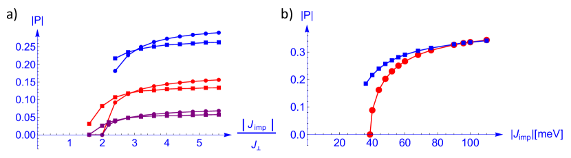
Figure 6: (Color online) Comparison between the approximate analytical (dots) and numerical (squares) values of the spiral order parameter $|P|$ [cf. Eq. (63)] for $XY-$spins on a cubic lattice with $L^{\,}_{x}=14$, $L^{\,}_{y}=14$, and $L^{\,}_{z}=32$. The impurity bonds form a superlattice. Panel (a) shows the results for the isotropic case $J^{\,}_{\parallel}/J^{\,}_{\perp}=1$ for three superlattices with the following basis vectors: (blue): $\boldsymbol{A}=(3,3,2)^{\mathsf{T}}$, $\boldsymbol{B}=(0,4,2)^{\mathsf{T}}$, and $\boldsymbol{C}=(4,0,2)^{\mathsf{T}}$, $n^{\,}_{\mathrm{imp}}=1/16$; (red): $\boldsymbol{A}=(5,3,2)^{\mathsf{T}}$, $\boldsymbol{B}=(3,4,4)^{\mathsf{T}}$, and $\boldsymbol{C}=(4,5,2)^{\mathsf{T}}$, $n^{\,}_{\mathrm{imp}}=1/32$; (purple): $A=(4,3,0)^{\mathsf{T}}$, $B=(0,4,3)^{\mathsf{T}}$, and $C=(5,0,2)^{\mathsf{T}}$, $n^{\,}_{\mathrm{imp}}=1/77$. Note that the magnitude $|P|$ of the spiral order parameter $P$ increases approximately linearly with $n^{\,}_{\mathrm{imp}}$. Panel (b) shows the dependence of $|P|$ on $|J^{\,}_{\mathrm{imp}}|$, for the parameters of YBaCuFeO₅ (cf.Eq. (64)), and a superlattice of density $n^{\,}_{\mathrm{imp}}=1/56$, with the basis $\boldsymbol{A}=(4,3,0)^{\mathsf{T}}$, $\boldsymbol{B}=(0,4,2)^{\mathsf{T}}$, and $\boldsymbol{C}=(4,0,2)^{\mathsf{T}}$.

The effective Ising Hamiltonian (56) is found to be very accurate once the impurity coupling $|J^{\,}_{\mathrm{imp}}|$ sufficiently exceeds the critical value $J^{\,}_{\mathrm{c}}$. This is illustrated by Fig. 5. Its four panels compare the approximate ground state obtained via the effective Ising Hamiltonian (56a) (shown on the left) with the ground state of the Hamiltonian (60) obtained via MC simulation (shown on the right). This is done for two strengths of impurity couplings and two different superlattices. We choose parameters such that both methods yield a spiral state, with $\boldsymbol{q}^{\,}_{\text{min}}=0$ minimizing the kernel $\Upsilon^{\,}_{\boldsymbol{q}}$. No coupling anisotropy ($J^{\,}_{\parallel}/J^{\,}_{\perp}=1$) was assumed in all these cases. Figures 5(a) and 5(b) correspond to the same superlattice, but different impurity strengths, $|J^{\,}_{\mathrm{imp}}|/J^{\,}_{\perp}=2.4$ and $4.8$, respectively. A spiral ground state is correctly predicted in both cases. However, while the canting angle ${\Delta\theta}$ at the impurity bonds and especially the spiral wave vector $Q$ are rather accurately predicted for strong impurity couplings $|J^{\,}_{\mathrm{imp}}|/J^{\,}_{\perp}=4.8$, they are underestimated by the effective theory when the impurity coupling $|J^{\,}_{\mathrm{imp}}|/J^{\,}_{\perp}=2.4$ comes relatively close to the threshold strength $J^{\,}_{\mathrm{c}}/J^{\,}_{\perp}=2$, cf. Eq. (27b). The agreement between the analytical approximation and the MC simulations improves with increasing $|J^{\,}_{\mathrm{imp}}|/J^{\,}_{\perp}$. This agrees with what one expects from the considerations of Sec. III.2. Indeed, assuming that all canting angles take the same value $\Delta\theta^{\,}_{\tilde{\boldsymbol{r}}}=\Delta\theta$, and assuming a superlattice of impurities, Eq. (41) takes the form

$$\Delta\theta=\frac{|J^{\,}_{\mathrm{imp}}|}{J^{\,}_{\mathrm{c}}-\left(\Gamma^{(0)}_{\boldsymbol{0}}\right)^{-2}\sum\limits_{\tilde{\boldsymbol{r}}\in\mathcal{L}\setminus\{\boldsymbol{0}\}}\Gamma^{(0)}_{\tilde{\boldsymbol{r}}}}\sin\Delta\theta.$$ (61)

As compared to the saddle point equation for a single impurity, Eq. (29), the denominator $J^{\,}_{\mathrm{c}}$ is shifted by the small correction

$$\left(\Gamma^{(0)}_{\boldsymbol{0}}\right)^{-2}\sum\nolimits_{\tilde{\boldsymbol{r}}\in\mathcal{L}\setminus\{\boldsymbol{0}\}}\Gamma^{(0)}_{\tilde{\boldsymbol{r}}}\sim n^{\,}_{\mathrm{imp}}\,\times\,\mathcal{O}(J^{\,}_{\perp},J^{\,}_{\parallel})\ll J^{\,}_{\mathrm{c}}.$$ (62)

When $|J^{\,}_{\mathrm{imp}}|/J^{\,}_{\mathrm{c}}$ is large, this renormalization has little effect on the solution of the saddle point equation, $\Delta\theta$, which will be close to $\pi$ in any case. However, when $|J^{\,}_{\mathrm{imp}}|/J^{\,}_{\mathrm{c}}$ is close to the threshold of 1, an effective reduction of $J^{\,}_{\mathrm{c}}$ (which is expected for superlattice that favor ferromagnetic Ising order) leads to an increase of $\Delta\theta$. For example, in Fig. 5(a), the value of the canting angle would $\Delta\theta=1.02$ according to Eq. (29), but increaes to $\Delta\theta=1.15$ after correcting it by Eq. (61).

Similar results are found for other superlattices. For instance, panels (c) and (d) show results for a denser superlattice, but with the same exchange couplings as in panels (a) and (b), respectively. In all panels of Fig. 5, the deviations from the local ferromagnetic order at non-impurity bonds are small, justifying a posteriori the spin-wave approximation used to derive the effective Ising Hamiltonian (56).

To quantify the quality of the approximations incurred when trading the microscopic Hamiltonian (60) for the effective Ising Hamiltonian (56), we compare the quantity

$$P\,\raisebox{0.85pt}{.}\raisebox{2.85pt}{.}\!\!=\,\frac{1}{L^{\,}_{x}\,L^{\,}_{y}\,\left(L^{\,}_{z}-1\right)}\sum_{\begin{subarray}{c}\boldsymbol{r}\in\Lambda\\ 1\leq r^{\,}_{z}\leq L^{\,}_{z}-1\end{subarray}}\sin\left(\phi^{\,}_{\boldsymbol{r}+\boldsymbol{z}}-\phi^{\,}_{\boldsymbol{r}}\right),$$ (63)

obtained from both Hamiltonians for several superlattices and various ratios $|J^{\,}_{\mathrm{imp}}|/J^{\,}_{\perp}$ in Fig. 6(a). Here, $L^{\,}_{x}$, $L^{\,}_{y}$, and $L^{\,}_{z}$ in Eq. (63) are the linear dimensions of the lattice, while $P$ is an order parameter for the magnetic spiral phase. On the right-hand side, the sine of the relative angle between $\widehat{\boldsymbol{S}}^{\,}_{\boldsymbol{r}}$ and $\widehat{\boldsymbol{S}}^{\,}_{\boldsymbol{r}+\boldsymbol{z}}$ is summed over all sites of the cubic host lattice $\Lambda$.

Figure6(a) shows how the value of $|P|$, evaluated on the minimal energy configuration, increases with increasing $|J^{\,}_{\mathrm{imp}}|/J^{\,}_{\perp}\geq J^{\,}_{\mathrm{c}}/J^{\,}_{\perp}$ for three superlattices of impurity bonds in an isotropic cubic lattice ($J^{\,}_{\parallel}/J^{\,}_{\perp}=1$), whereby all superlattices were chosen so that they induce a spiral state. At relatively large $|J^{\,}_{\mathrm{imp}}|/J^{\,}_{\perp}$, the results for $|P|$ from the effective Ising Hamiltonian (56) (dots) are close to those obtained from the microscopic simulation of Hamiltonian (60) (squares), up to corrections of order $n^{\,}_{\mathrm{imp}}$, as anticipated in the discussion around Eq. (42). However, as $|J^{\,}_{\mathrm{imp}}|$ approaches $J^{\,}_{\mathrm{c}}$ from above, deviations become stronger, as we discussed after Eq. (61). In this regime the double-well potential defining the Ising degrees of freedom associated with the canting pattern becomes very shallow. Thus, even relatively weak contributions from neighboring impurities, $\Xi^{\,}_{\tilde{\boldsymbol{r}}}$, can stabilize and enhance the local canting ${\Delta\theta}$ and strengthen the spiral wave vector beyond the approximations we used to derive the effective model. For the same reason of mutual stabilization, we still find a finite spiral order, $P\neq 0$, even when $J^{\,}_{\mathrm{imp}}/J^{\,}_{\perp}\lesssim J^{\,}_{\mathrm{c}}/J^{\,}_{\perp}=2$.

IV.3 Spiral phase in a realistic model for YBaCuFeO₅

It was argued in Ref. Scaramucci et al., 2018 that the magnetic degrees of freedom in the insulator YBaCuFeO₅ realize a close cousin of Hamiltonian (60), in that $J^{\,}_{\perp}>0$ is to be replaced by two distinct values $J^{\prime}_{\perp}>0$ and $J^{\prime\prime}_{\perp}>0$ depending on the parity of the $z$ component of the coordinate $\boldsymbol{r}$ of the cubic lattice. From the estimates for $J^{\,}_{\parallel}>0$, $J^{\prime}_{\perp}>0$, $J^{\prime\prime}_{\perp}>0$, and $J^{\,}_{\mathrm{imp}}<0$ made in Ref. Scaramucci et al., 2018 we have borrowed the values

$$\begin{split}&J^{\,}_{\parallel}=28.9\text{meV},\\ &J^{\,}_{\mathrm{imp}}=-95.8\text{meV},\\ &J^{\,}_{\perp}\equiv(J^{\prime}_{\perp}+J^{\prime\prime}_{\perp})/2=4.1\text{meV}.\end{split}$$ (64)

Figure 6(b) compares the dependence of the magnitude $|P|$ of the spiral order parameter $P$ defined in Eq. (63) on $J^{\,}_{\mathrm{imp}}$ for the microscopic Hamiltonian (60) (squares) with that for the effective Ising Hamiltonian (56) (dots) for the case when the impurity bonds form a superlattice that stabilizes a long-range spiral order. Again, good agreement is found once the the impurity bond strength is sufficiently stronger than the threshold, in which case the two possible canting patterns form robust local minima of the Hamiltonian. This is indeed the case in YBaCuFeO₅, where $|J^{\,}_{\mathrm{imp}}|/J^{\,}_{\perp}\approx 23>J^{\,}_{\mathrm{c}}/J^{\,}_{\perp}\approx 9.4$.

IV.4 Dependence of the ground state on the superlattice of impurity bonds

We now illustrate how the choice made for the superlattice of impurity bonds affects the ground state. We use again the values (64) corresponding to ideal YBaCuFeO₅ when defining the effective Ising Hamiltonian (56) and the microscopic Hamiltonian (60).

We consider two superlattices of impurity bonds. They are chosen such that $\Upsilon^{\,}_{\boldsymbol{q}}$ has a global minimum at $\boldsymbol{q}^{\,}_{\text{min}}=0$ for one, and at $\boldsymbol{q}^{\,}_{\text{min}}=\boldsymbol{C}^{\star}/2$ for the other, cf. Fig. 7). Furthermore, both superlattices are chosen such that they share with YBaCuFeO₅ the additional property that impurity bonds only occur between every other plane.

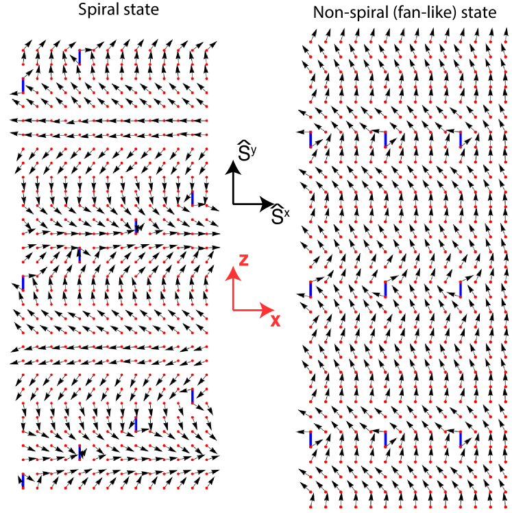
Figure 7: (Color online) Ground states obtained from the microscopic Hamiltonian (60). We choose the values of the exchange couplings motivated by those calculated for YBaCuFeO₅, cf. Eq. (64), and with impurity bonds forming a regular superlattice. The ground state depends qualitatively on the superlattice: (a) A superlattice with basis vectors $\boldsymbol{A}=(4,3,0)^{\mathsf{T}}$, $\boldsymbol{B}=(0,4,2)^{\mathsf{T}}$, and $\boldsymbol{C}=(4,0,2)^{\mathsf{T}}$ ($n^{\,}_{\mathrm{imp}}=1/56$) results in a magnetic spiral. (b) A superlattice with basis vectors $\boldsymbol{A}=(5,0,0)^{\mathsf{T}}$, $\boldsymbol{B}=(0,5,0)^{\mathsf{T}}$, and $\boldsymbol{C}=(0,1,2)^{\mathsf{T}}$ ($n^{\,}_{\mathrm{imp}}=1/50$) results in a non-spiral (fan-like) ground state. In this case, $\Upsilon^{\,}_{\boldsymbol{q}}$ (Eq. 56c) takes its minimum at $\boldsymbol{q}^{\,}_{\text{min}}=\boldsymbol{C}^{\star}/2$, which yields a non-spiral ground state (with $Q=0$).

The essential difference between the two superlattices lies in the relative position of nearest-neighbor impurity bonds. In the first lattice, the majority of nearest-neighbor impurity bonds is ferromagnetically coupled. This favors a ferromagnetic Ising phase in the effective Ising Hamiltonian (56), i.e., a spiral magnetic phase. In the second lattice, the majority of nearest-neighbor impurity bonds is antiferromagnetically coupled. This favors a layered antiferromagnetic Ising ground state of the effective Ising Hamiltonian (56), and thus, a fan-like magnetic order with no net winding of the spins, whereby the orientation of the magnetization of the layers alternate between even and odd pairs of planes.

We have verified using MC simulations of the microscopic Hamiltonian (60) that the long-range spiral order, which is present when the impurity bonds are arranged in certain Bravais superlattices, is robust to weak distortions of that superlattice, as expected on theoretical grounds.

IV.5 Limit of dilute impurities

Next we analyze the limits of very dilute tetragonal, face-centered-cubic, and body-centered-cubic superlattices of impurity bonds. These are tractable analytically. We shall show that ferromagnetic order prevails at the level of the Ising degrees of freedom associated with local cantings for dilute face-centered-cubic and body-centered-cubic superlattices of impurity bonds. This is to say that spiral order for the underlying $XY$ spin degrees of freedom prevails for these diluted superlattices of impurity bonds. The results obtained here will also be useful for the study of random impurity bonds in Sec. V.

IV.5.1 Cubic superlattices

We assume that the impurity bonds occupy a cubic sublattice $\mathcal{L}$ of the cubic host lattice $\Lambda$. As it turns out, this case supports antiferromagnetic order in the Ising model. Some results of this calculation will later help us to establish that the disordered case, in contrast, orders ferromagnetically.

If the cubic host lattice $\Lambda$ and the superlattice $\mathcal{L}$ are finite and not too large, it is possible to calculate the energy (52a) for all Ising spin configurations by exact evaluation of the Ising kernel $J^{(\mathrm{I})}_{\tilde{\boldsymbol{r}}-\tilde{\boldsymbol{r}}^{\prime}}$ defined in Eq. (52c). In the thermodynamic limit, $|\Lambda|\to\infty$, with $n^{\,}_{\mathrm{imp}}$ held fixed, this approach is not possible anymore. Instead, we shall restrict ourselves to a few long range-ordered Ising configurations that are likely candidates for the ground state, and compare their energies.

The ferromagnetic Ising configuration is described by

$$\sigma^{\mathrm{F}}_{\tilde{\boldsymbol{r}}}\,\raisebox{0.85pt}{.}\raisebox{2.85pt}{.}\!\!=\,1,\qquad\frac{1}{|\Lambda|}\sum_{\tilde{\boldsymbol{r}}\in\mathcal{L}}\sigma^{\mathrm{F}}_{\tilde{\boldsymbol{r}}}=n^{\,}_{\mathrm{imp}}.$$ (65a)

The most relevant competing states have ferromagnetic order in plane (as favored by the ferromagnetic interactions in the $$xy- z \tilde{\boldsymbol{r}}=(\tilde{x},\tilde{y},\tilde{z})$$plane), but antiferromagnetic order along the -axis. We consider the family of states defined by []

$$\begin{split}\sigma^{\mathrm{AF}(m)}_{\tilde{\boldsymbol{r}}}\,\raisebox{0.85pt}{.}\raisebox{2.85pt}{.}\!\!=\,(-1)^{\lfloor\tilde{z}/m\,\ell\rfloor},\qquad\frac{1}{|\Lambda|}\sum_{\tilde{\boldsymbol{r}}\in\mathcal{L}}\sigma^{\mathrm{AF}(m)}_{\tilde{\boldsymbol{r}}}=0,\end{split}$$ (65b)

which describes a sequence of stacks of $$m\geq 1$$ layers, whose magnetization alternates. Here,

$$\ell\equiv n^{-1/3}_{\mathrm{imp}}$$ (65c)

denotes the lattice spacing of the cubic superlattice, and $\lfloor\tilde{z}/m\,\ell\rfloor$ returns the integer part of the fraction $\tilde{z}/m\,\ell$.

After subtraction of the three constants $E^{\,}_{\mathrm{FM}}$, $E({\Delta\theta})\,|\mathcal{L}|$, and $-\gamma\,n^{\,}_{\mathrm{imp}}/2J^{\,}_{\perp}$ on the right-hand side of Eq. (52a), the energy per impurity bond of the configurations $\mathrm{C}\in\left\{\mathrm{F,AF}(m)\right\}$ is given by

$$\varepsilon^{\mathrm{C}}_{\mathcal{L}}=-\frac{\gamma}{2}\left(\sum_{\tilde{\boldsymbol{r}}\in\mathcal{L}\setminus\{\boldsymbol{0}\}}\Gamma^{(0)}_{\tilde{\boldsymbol{r}}}\,f^{\mathrm{C}}(\tilde{z})+\frac{n^{\,}_{\mathrm{imp}}}{J^{\,}_{\perp}}\,\delta^{\,}_{\mathrm{C,F}}\right),$$ (66a)

where the spin autocorrelation function

$$f^{\mathrm{C}}(\tilde{\boldsymbol{r}})\equiv\langle\sigma^{\,}_{\tilde{\boldsymbol{r}}^{\prime}}\,\sigma^{\,}_{\tilde{\boldsymbol{r}}^{\prime}+\tilde{\boldsymbol{r}}}\rangle^{\,}_{\tilde{\boldsymbol{r}}^{\prime}}=f^{\mathrm{C}}(\tilde{z})$$ (66b)

only depends on the difference in the $$\tilde{z} \langle\dots\rangle_{\tilde{\boldsymbol{r}}^{\prime}} {\tilde{\boldsymbol{r}}^{\prime}} \mathcal{L} \mathrm{F} \mathrm{AF(1)}$$ coordinate, owing to Eq. (65). Here, denotes the average over the sites of the superlattice . For configurations and , it is given by

$$f^{\mathrm{F}}(\tilde{z})=1,\qquad f^{\mathrm{AF(1)}}(\tilde{z})=(-1)^{\tilde{z}/\ell}.$$ (66c)

In the dilute limit $n^{\,}_{\mathrm{imp}}\to 0$, the typical distance between a pair of nearest-neighbor impurities is large. Hence, the typical pair-wise interaction $\Gamma^{(0)}_{\tilde{\boldsymbol{r}}}$ tends to the dipolar form (14) and can be safely used to evaluate $\varepsilon^{\mathrm{AF}(m)}_{\mathcal{L}}$ up to corrections which are subleading in the limit $n^{\,}_{\mathrm{imp}}\to 0$. The case of the ferromagnetic configuration is more subtle, however. Indeed, a naive use of Eq. (14) would suggest that the first term in the right-hand side of Eq. (66a) vanishes due to the sum over symmetry related directions, while in fact it does not. This is due to corrections to the dipolar interaction (14) that scale as the inverse of the volume, but add up to a finite contribution when summed with equal signs over the whole superlattice. In the case of an isotropically shaped, cubic sample with $L^{\,}_{x}=L^{\,}_{y}=L^{\,}_{z}$ and isotropic interactions $J^{\,}_{\parallel}=J^{\,}_{\perp}\equiv J$, the computation can be done exactly, using the fact that upon averaging over all the permutations $k^{\,}_{x}\to k^{\,}_{y}\to k^{\,}_{z}\to k^{\,}_{x}$ the kernel $\hat{\Gamma}_{\boldsymbol{k}}^{(0)}$ (LABEL:eq:_def_Gammas_and_hat_Gammas_b) reduces to $1/3J$. Using $f^{\mathrm{F}}(z)=1$ this allows us to evaluate the lattice sum exactly for any impurity density as

$$\sum_{\tilde{\boldsymbol{r}}\in\mathcal{L}\setminus\{\boldsymbol{0}\}}\Gamma^{(0)}_{\tilde{\boldsymbol{r}}}f^{\mathrm{F}}(\tilde{z})= \,\frac{1}{3J\,|\Lambda|}\sum_{\tilde{\boldsymbol{r}}\in\mathcal{L}\setminus\{\boldsymbol{0}\}}\sum_{\boldsymbol{k}\in\mathrm{BZ}(\Lambda)\setminus\{\boldsymbol{0}\}}e^{\mathrm{i}\boldsymbol{k}\cdot\tilde{\boldsymbol{r}}}$$

$$= \,\frac{1}{3J\,|\Lambda|}\sum_{\tilde{\boldsymbol{r}}\in\mathcal{L}\setminus\{\boldsymbol{0}\}}\left(|\Lambda|\,\delta^{\,}_{\tilde{\boldsymbol{r}},\boldsymbol{0}}-1\right)$$

$$= \,-\frac{1}{3J}\frac{|\mathcal{L}|-1}{|\Lambda|}$$

$$= \,-\frac{n^{\,}_{\mathrm{imp}}}{3J}+\mathcal{O}\left(\frac{1}{|\Lambda|}\right).$$ (67)

This finite, negative contribution disfavors the ferromagnet, in analogy to demagnetizing factors known from standard magnetic dipolar systems. Restricting ourselves to the isotropic case and inserting Eq. (67) into Eq. (66a), we obtain the energy per impurity

$$\varepsilon^{\mathrm{F}}_{\mathcal{L}}=-\frac{1}{3}\,\frac{\gamma\,n^{\,}_{\mathrm{imp}}}{J^{\,}_{\perp}}.$$ (68)

More generally, it is useful to cast the energy (66a) for the ferromagnetic configuration (65a) of the Ising variables in a different form, namely,

$$\frac{\varepsilon^{\mathrm{F}}_{\mathcal{L}}}{(\gamma/2)}= \,-\sum_{\tilde{\boldsymbol{r}}\in\mathcal{L}}\Gamma^{(0)}_{\tilde{\boldsymbol{r}}}+\Gamma^{(0)}_{\tilde{\boldsymbol{r}}=\boldsymbol{0}}-\frac{n^{\,}_{\mathrm{imp}}}{J^{\,}_{\perp}}$$

$$= \,-\frac{1}{|\Lambda|}\sum_{\tilde{\boldsymbol{r}}\in\mathcal{L}}\sum_{\boldsymbol{k}\in\mathrm{BZ}(\Lambda)}e^{\mathrm{i}\boldsymbol{k}\cdot\tilde{\boldsymbol{r}}}\,\hat{\Gamma}^{(0)}_{\boldsymbol{k}}+\Gamma^{(0)}_{\tilde{\boldsymbol{r}}=\boldsymbol{0}}-\frac{n^{\,}_{\mathrm{imp}}}{J^{\,}_{\perp}}$$

$$= \,-\frac{|\mathcal{L}|}{|\Lambda|}\sum_{\begin{subarray}{c}\boldsymbol{k}\in\mathrm{BZ}(\Lambda)\\ \boldsymbol{k}\in\mathcal{L}^{\star}\end{subarray}}\hat{\Gamma}^{(0)}_{\boldsymbol{k}}+\Gamma^{(0)}_{\tilde{\boldsymbol{r}}=\boldsymbol{0}}-\frac{n^{\,}_{\mathrm{imp}}}{J^{\,}_{\perp}},$$ (69)

where the reciprocal lattice $\mathcal{L}^{\star}$ of $\mathcal{L}$ enters through the identity (55), $\hat{\Gamma}^{(0)}_{{\boldsymbol{k}}{\neq\boldsymbol{0}}}$ has been defined in Eq. (LABEL:eq:_def_Gammas_and_hat_Gammas_b) and we recall that $\hat{\Gamma}^{(0)}_{\boldsymbol{k}=\boldsymbol{0}}=0$. The sum over $\boldsymbol{k}$ thus contains $|\Lambda|/|{\cal L}|-1=1/n^{\,}_{\mathrm{imp}}-1$ terms. Note that the self-interaction $\Gamma^{(0)}_{\tilde{\boldsymbol{r}}=\boldsymbol{0}}$ [cf.  Eq. 32)], which appears also in the single impurity energy, is subtracted on the right-hand side of Eq. (69).

We point out an important difference between the present effective dipolar problem and genuine magnetic dipoles. Genuine dipolar interactions are mediated by magnetic fields which extend everywhere in space, beyond the boundaries of the sample. Therefore they only depend on the relative position of two spins, irrespective of where the spins are deep in the bulk, or close to a surface of a finite sample. However, this is not so in our case where the dipolar interactions arise through the mediation of spin waves, which are confined to the sample. Accordingly, the interactions involving Ising spins at the periphery of the sample are not exactly the same as those for bulk Ising spins with the same relative position. More importantly there are no magnetic stray fields beyond the sample. In real dipolar magnets those store a lot of magnetic energy, which is avoided in the ground state by domain formation. The unavoidable presence of domains complicates the computation of the energy density. In particular, the evaluation for a homogeneously magnetized sample yields a shape dependent result, a fact that is reflected in the ambiguity of the value of the Fourier transform of the dipolar interactions Eq. (LABEL:eq:_def_Gammas_and_hat_Gammas_b) in the limit $\boldsymbol{k}\to 0$. In the present case, however, such problems do not arise, since the spin-wave mediated interaction is such that $\hat{\Gamma}^{(0)}_{\boldsymbol{k}=\boldsymbol{0}}=0$. This eliminates the potential ambiguity and therefore eliminates the shape dependence. We also do not expect the effective dipolar interactions to induce domains, in contrast to genuine ferromagnets.

Performing an analogous calculation to the one above yields for the antiferromagnet $\mathrm{AF}(1)$

$$\frac{\varepsilon^{\mathrm{AF}(1)}_{\mathcal{L}}}{(\gamma/2)}= \,-\sum_{\tilde{\boldsymbol{r}}\in\mathcal{L}}\Gamma^{(0)}_{\tilde{\boldsymbol{r}}}\,(-1)^{\lfloor\tilde{z}/\ell\rfloor}+\Gamma^{(0)}_{\tilde{\boldsymbol{r}}=\boldsymbol{0}}$$

$$= \,-\frac{|\mathcal{L}|}{|\Lambda|}\sum_{\begin{subarray}{c}\boldsymbol{k}\in\mathrm{BZ}(\Lambda)\\ \boldsymbol{k}+(0,0,\pi/\ell)^{\mathsf{T}}\in\mathcal{L}^{\star}\end{subarray}}\hat{\Gamma}^{(0)}_{\boldsymbol{k}}+\Gamma^{(0)}_{\tilde{\boldsymbol{r}}=\boldsymbol{0}}.$$ (70)

Even though the quantitative mapping from the $XY$ Hamiltonian (1) to the effective Ising Hamiltonian (52) only holds for low densities of impurity bonds, it is useful to study the effective Ising Hamiltonian (52) in its own right, i.e., without requiring the impurity bonds to be dilute.

A maximally dense superlattice is defined by

$$\ell=1,\qquad\mathcal{L}=\Lambda,\qquad n^{\,}_{\mathrm{imp}}=\frac{|\mathcal{L}|}{|\Lambda|}=1.$$ (71)

For such a lattice, one finds the ferromagnetic (F) and antiferromagnetic [AF(1)] states to be degenerate,

$$\frac{\varepsilon^{\mathrm{F}}_{\mathcal{L}}-\varepsilon^{\mathrm{AF}(1)}_{\mathcal{L}}}{(\gamma/2)\,n^{\,}_{\mathrm{imp}}}=\,\hat{\Gamma}^{(0)}_{\boldsymbol{k}=(0,0,{\pi})^{\mathsf{T}}}-\hat{\Gamma}^{(0)}_{\boldsymbol{k}=\boldsymbol{0}}-\frac{1}{J^{\,}_{\perp}}=0,$$ (72)

since, cf. Eqs. (LABEL:eq:_def_Gammas_and_hat_Gammas_b) and (13c),

$$\hat{\Gamma}^{(0)}_{(0,0,k^{\,}_{z})^{\mathsf{T}}}=\frac{1-\delta^{\,}_{k^{\,}_{z},0}}{J^{\,}_{\perp}},$$ (73)

The identity (73) obeyed by the kernel (LABEL:eq:_def_Gammas_and_hat_Gammas_b) can be used together with the expression (56a) and the fact that only $\boldsymbol{q}$ of the form $(0,0,k^{\,}_{z})^{\mathsf{T}}$ enter it, to show that for a maximally dense superlattice all antiferromagnetic states $\mathrm{AF}(m)$ are degenerate with the ferromagnet. More generally, it is shown in appendix A that the ferromagnet is degenerate with any Ising configuration in which the spins in every given plane at fixed $z$ coordinate are ferromagnetically aligned, irrespective of the relative orientation of the magnetization of different planes.

This degeneracy is, however, lifted at finite dilution, whereby the way in which the dilution is realized is crucial.

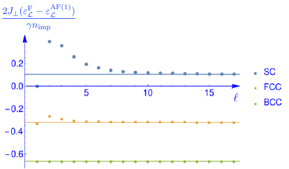
Figure 8: (Color online) Dependence of the energy difference between the Ising ferromagnetic (F) and antiferromagnetic [AF($1$)] states on the linear size $\ell$ of the unit cell of the superlattice for different classes of superlattices. Blue dots represent a simple cubic (SC) superlattice with the basis vectors $(\ell,0,0)$, $(0,\ell,0)$, and $(0,0,\ell)$. Yellow squares represent a face centered cubic (FCC) superlattice with lattice vectors $(\ell,\ell,0)$, $(\ell,0,\ell)$, and $(0,\ell,\ell)$. Green diamonds represent body centered cubic (BCC) superlattices with the lattice vectors $(\ell,\ell,\ell)$, $(\ell,-\ell,\ell)$, and $(\ell,\ell,-\ell)$. The correspondingly colored horizontal solid lines represent the dilute limit $\ell\to\infty$ of these energy differences for each superlattice.

For example, diluting the impurity density $n^{\,}_{\mathrm{imp}}$ by maintaining a cubic superlattice, but increasing its integer lattice spacing $\ell$ disfavors the ferromagnetic state. This is illustrated in Fig. 8, where we plot the energies per impurity as a function of superlattice spacing $\ell$. For small $\ell$, the energy difference is obtained from the representations (69) and (IV.5.1). In the dilute limit, $n^{\,}_{\mathrm{imp}}=\ell^{-3}\to 0$, the reciprocal lattice $\mathcal{L}^{\star}$ only contains small wavevectors, and we may replace $1-\cos k^{\,}_{i}$ (where $k^{\,}_{i}=2\pi\,n^{\,}_{i}/\ell$) in the kernel (LABEL:eq:_def_Gammas_and_hat_Gammas_b) by $(2\pi\,n^{\,}_{i})^{2}/2\ell^{2}$ with $n^{\,}_{i}\in\mathbb{Z}$ for $i=x,y,z$, i.e.,

$$\frac{\varepsilon^{\mathrm{F}}_{\mathcal{L}}-\varepsilon^{\mathrm{AF}(1)}_{\mathcal{L}}}{(\gamma/2)\,n^{\,}_{\mathrm{imp}}}\to\frac{\delta(\alpha)}{J^{\,}_{\perp}}$$ (74a)

where the exchange anisotropy parameter $$\alpha$$ was defined in Eq. (35), and

$$\begin{split}\delta(\alpha)\,\raisebox{0.85pt}{.}\raisebox{2.85pt}{.}\!\!=\,&\,-1-\sum_{\boldsymbol{n}\in\mathbb{Z}^{3}\setminus{\{\boldsymbol{0}\}}}\frac{n^{2}_{z}}{\alpha\left(n^{2}_{x}+n^{2}_{y}\right)+n^{2}_{z}}\\ &\,+\sum_{\boldsymbol{n}\in\mathbb{Z}^{3}}\frac{\left(n^{\,}_{z}-1/2\right)^{2}}{\alpha\left(n^{2}_{x}+n^{2}_{y}\right)+(n^{\,}_{z}-1/2)^{2}}.\end{split}$$ (74b)

The sum over $n^{\,}_{z}$ can be carried out explicitly,

$$\delta(\alpha)=\sum_{\boldsymbol{n}\in\mathbb{Z}^{2}\setminus\{\boldsymbol{0}\}}\frac{2\pi\,\sqrt{\alpha\,(n^{2}_{x}+n^{2}_{y})}}{\sinh\left(2\pi\sqrt{\alpha(n^{2}_{x}+n^{2}_{y})}\right)}.$$ (75)

Hence, $\delta(\alpha)$ is always positive. For the isotropic limit $\alpha=1$, one finds $\delta(1)\approx 0.1042$.

Alternatively, one can calculate the antiferromagnetic energy directly in real space using the dipolar form (14). This can be used to calculate the energies of other antiferromagnetic states $\mathrm{AF}(m)$, which all scale as

$$\frac{\varepsilon^{\mathrm{AF}(m)}_{\mathcal{L}}}{(\gamma/2)\,n^{\,}_{\mathrm{imp}}}=-\frac{c^{\,}_{m}}{J^{\,}_{\perp}}.$$ (76)

From the results (68, 74a) it follows that $c^{\,}_{1}=\delta(1)+2/3$, while one finds the higher $c^{\,}_{m}$’s to decrease monotonically with increasing $m$. From this we conclude that a dilute cubic superlattice orders antiferromagnetically with layer magnetizations that alternate in sign ($m=1$).

IV.5.2 Dilute tetragonal, face-centered, and body-centered tetragonal superlattices

One readily generalizes the above calculation to tetragonal superlattices $\mathcal{L}$ with unit vectors $(A\ell,0,0)^{\mathsf{T}}$, $(0,A\ell,0)^{\mathsf{T}}$, $(0,0,C\ell)^{\mathsf{T}}$, where $A$ and $C$ are fixed integers while the integer-valued dilution parameter $\ell$ will be taken to infinity. This case is obtained from that of a cubic lattice by substituting

$$n^{\,}_{\mathrm{imp}}\to\frac{1}{A^{2}\,C\,\ell^{3}},\qquad\alpha\to\frac{J^{\,}_{\parallel}}{J^{\,}_{\perp}}\,\frac{C^{2}}{A^{2}},$$ (77)

in Eq. (74a) and (74b). Independently of the ratio $C/A$ of the tetragonal superlattice, the Ising antiferromagnetic state AF(1) is favored over the Ising ferromagnetic state F.

However, similarly as in lattice problems of physical electric or magnetic dipoles Luttinger and Tisza (1946) where the interactions have reversed global sign, a different ground state is found in dilute body-centered or face-centered tetragonal lattices. The difference arises because closest neighbors in these lattices have a stronger tendency to have ferromagnetic interactions than in simple tetragonal lattices. For the face-centered tetragonal lattice, the basis vectors are $(A,A,0)$, $(A,0,C)$, and $(0,A,C)$. The corresponding dual basis vectors in reciprocal space are $\boldsymbol{e}^{\,}_{1}=\pi(1/A,1/A,-1/C)$, $\boldsymbol{e}^{\,}_{2}=\pi(1/A,-1/A,1/C)$, and $\boldsymbol{e}^{\,}_{3}=\pi(-1/A,1/A,1/C)$. Their linear combinations with integer coefficients span the reciprocal lattice $\mathcal{L}^{\star}$. It is convenient to represent a generic reciprocal lattice vector $\boldsymbol{G}\in\mathcal{L}^{\star}$ as $\boldsymbol{G}=n^{\,}_{1}\,\boldsymbol{e}^{\,}_{1}+n^{\,}_{2}\,\boldsymbol{e}^{\,}_{2}+n^{\,}_{3}(\boldsymbol{e}^{\,}_{2}+\boldsymbol{e}^{\,}_{3})$. With this choice, the asymptotic energy difference between the ferromagnetic and the antiferromagnetic states in the infinite dilution limit $n^{\,}_{\mathrm{imp}}\to 0$ can be written as

$$\frac{\varepsilon^{\mathrm{F}}_{\mathcal{L}}-\varepsilon^{\mathrm{AF}(1)}_{\mathcal{L}}}{(\gamma/2)\,n^{\,}_{\mathrm{imp}}}=-\frac{1}{J^{\,}_{\perp}}-\sum_{\boldsymbol{n}\in\mathbb{Z}^{3}\setminus{\{\boldsymbol{0}\}}}\frac{g^{\,}_{\boldsymbol{n}}}{J^{\,}_{\perp}}+\sum_{\boldsymbol{n}\in\mathbb{Z}^{3}}\frac{g^{\,}_{{(n_{1},n_{2},n_{3}+\frac{1}{2})}}}{J^{\,}_{\perp}},$$ (78a)

where

$$g^{\,}_{\boldsymbol{n}}\,\raisebox{0.85pt}{.}\raisebox{2.85pt}{.}\!\!=\,\frac{(n^{\,}_{1}-n^{\,}_{2}-2n^{\,}_{3})^{2}}{\alpha\left[(n^{\,}_{1}+n^{\,}_{2})^{2}+(n^{\,}_{1}-n^{\,}_{2})^{2}\right]+(n^{\,}_{1}-n^{\,}_{2}-2n^{\,}_{3})^{2}},$$ (78b)

where for vanishing wavevector we have to set $g^{\,}_{\boldsymbol{0}}=0$. Carrying out the sum over $n^{\,}_{3}$ one finds

$$\begin{split}\frac{\varepsilon^{\mathrm{F}}_{\mathcal{L}}-\varepsilon^{\mathrm{AF}(1)}_{\mathcal{L}}}{(\gamma/2)\,n^{\,}_{\mathrm{imp}}}=&\,\sum_{\boldsymbol{n}\in\mathbb{Z}^{2}\setminus\{\boldsymbol{0}\}}\frac{(-1)^{n^{\,}_{1}-n^{\,}_{2}}}{J^{\,}_{\perp}}\\ &\,\times\frac{\pi\,\sqrt{2\alpha\,\left(n^{2}_{1}+n^{2}_{2}\right)}}{\sinh\left(\pi\sqrt{2\alpha\,\left(n^{2}_{1}+n^{2}_{2}\right)}\right)}.\end{split}$$ (79)

In the isotropic case $\alpha=1$, the energy difference is negative $J(\varepsilon^{\mathrm{F}}_{\mathcal{L}}-\varepsilon^{\mathrm{AF}(1)}_{\mathcal{L}})/(\gamma/2)\,n^{\,}_{\mathrm{imp}}=-0.3218$, so the ferromagnetic order prevails.

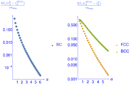
Figure 9: (Color online) Dependence of the energy difference between the Ising ferromagnetic state (F) and antiferromagnetic state [AF(1)] as a function of $\alpha\equiv J^{\,}_{\parallel}/J^{\,}_{\perp}$ [recall Eq. (35)] for a simple cubic superlattice (right panel) in the large dilution limit. The left panel shows the energy difference between the Ising antiferromagnetic state [AF(1)] and ferromagnetic state (F) for face centered superlattices (yellow squares) and a body centered superlattice (green diamonds). Independently of the value of $\alpha$, the antiferromagnetic state has lower energy for simple cubic superlattices while the ferromagnetic state has lower energy for face and body centered superlattices.

For body-centered tetragonal lattices one finds the same expression, but with the replacement $2\alpha\to\alpha$. The energy difference turns out to be always negative for any value of $\alpha$, as seen in Fig. 9. Thus, in both these types of superlattices the ferromagnetic state is favored over the layered antiferromagnetic state, whatever the tetragonal aspect ratio.

V Random impurities: dilute limit

In this section, we study randomly distributed impurities that occupy a fraction $n^{\,}_{\mathrm{imp}}$ of the sites of the cubic host lattice $\Lambda$. We assume again that the relevant contenders for the ground state are given by Eqs. (65a) and (65b). In Eq. (65b), we set $\ell=1$, since only the lattice constant of the cubic host lattice $\Lambda$ is relevant. These configurations are expected to come reasonably close to the true ground state and the relevant competing metastable configurations. However, they will differ in the orientation of a few spins from the simple configurations (65a) and (65b). The relative fraction of these spins becomes increasingly small as $n^{\,}_{\mathrm{imp}}\to 0$, as discussed below.

If the impurities are distributed randomly according to a Poisson process, the average energy per impurity bond of the trial configurations $\mathrm{C}=\mathrm{F},\mathrm{AF}(m)$ is given by

$$\varepsilon^{\mathrm{C}}_{\mathrm{dis}}=-\frac{\gamma}{2}\,n^{\,}_{\mathrm{imp}}\left(\sum_{{\boldsymbol{r}}\in\Lambda}\Gamma^{(0)}_{{\boldsymbol{r}}}\,f^{\mathrm{C}}({z})+\frac{1}{J^{\,}_{\perp}}\,\delta^{\,}_{\mathrm{C,F}}\right),$$ (80)

since any site ${\boldsymbol{r}}$ of the cubic host lattice $\Lambda$ is the lower end of an impurity bond with probability $n^{\,}_{\mathrm{imp}}$, independently of the location of other impurities. From this observation, one might at first conclude that the antiferromagnetic state should dominate again. However, the above consideration does not treat correctly impurities located at short distances from each other. On the one hand, rare pairs of impurities that are located much closer to each other than the average separation $n^{-1/3}_{\mathrm{imp}}$ do not follow the pattern (65a) and (65b), but simply optimize their mutual interaction energy, irrespective of the global ordering pattern. Since such pairs nevertheless contribute a finite fraction to the total energy estimated above, they must be corrected for, which will turn out to favor the ferromagnetic ordering. This conclusion will become clear below, as a corollary to the discussion of another short-distance effect, which we will consider first.

Impurity distributions in real materials are usually not simply governed by a Poisson process, but rather, one should expect them to exhibit some short-range correlations. For example, in the case of YBaCuFeO₅ impurity bonds arise due to chemical disorder which occasionally replaces the usual Cu-Fe pairs on bonds along its crystallographic $c$-axis by impurity configurations consisting in Fe-Fe or Cu-Cu pairs. Fe-Fe pairs differ from Fe-Cu pairs by the sign and magnitude of the resulting magnetic exchange constant. Moreover, both Fe-Fe and Cu-Cu pairs differ from Fe-Cu pairs in their local charge density. The resulting Coulomb repulsion between such impurity configurations thus suppresses the occurence of pairs of impurities at short distances. In a crude manner, we can mimic this effect by a hard constraint on the minimal distance between impurities, excluding distance vectors with $|{\boldsymbol{r}}|\leq R$. With such a constraint the average energy per impurity (80) is modified to

$$\varepsilon^{\mathrm{C}}_{\mathrm{dis}}(R)=-\frac{\gamma}{2}\,n^{\,}_{\mathrm{imp}}\,\left(\sum_{\begin{subarray}{c}{\boldsymbol{r}}\in\Lambda\\ |{\boldsymbol{r}}|>R\end{subarray}}\Gamma^{(0)}_{{\boldsymbol{r}}}\,f^{\mathrm{C}}({z})+\frac{1}{J^{\,}_{\perp}}\,\delta^{\,}_{\mathrm{C,F}}\right).$$ (81)

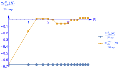
Figure 10: (Color online) Dependence on $R$ of $\varepsilon^{\mathrm{C}}_{\mathrm{dis}}(R)/(\gamma\,n^{\,}_{\mathrm{imp}})$ defined in Eq. (81) for isotropic couplings $J^{\,}_{\perp}=J^{\,}_{\parallel}\equiv J$ for the ferromagnetic ($\mathrm{C}=\mathrm{F}$, blue dots) and the layered antiferromagnetic state ($\mathrm{C}=\mathrm{AF}(1)$, yellow squares). Energies are given in units of $J$.

Note that for $R=0$ these energies are simply $n^{\,}_{\mathrm{imp}}$ multiplying the energy per impurity $\varepsilon_{\mathcal{L}=\Lambda}^{\mathrm{C}}(R)$ of a maximally dense system of impurities, recall Eq. (66a). As we have shown in the previous section, those energies are all degenerate. Since the sum over $\boldsymbol{r}$ in Eq. (81) is dominated by small $|\boldsymbol{r}|$, even a small $R$ of the order of one lattice constant will have a decisive effect and lifts this degeneracy. In Fig. 10, we plot as a function of $R$ the average energies $2\varepsilon^{\mathrm{F}}_{\mathrm{dis}}(R)/(\gamma\,n^{\,}_{\mathrm{imp}})$ and $2\varepsilon^{\mathrm{AF}(m=1)}_{\mathrm{dis}}(R)/(\gamma\,n^{\,}_{\mathrm{imp}})$ of the two most relevant competing states. Already, for the smallest effective exclusion radius of $R\geq R^{\,}_{\mathrm{c}}=1$ (in units of the host cubic lattice spacing), we find that the ferromagnetic state (and thus $XY$ spiral order) wins over the antiferromagnetic state (i.e., $XY$ fan order). This numerical result can be understood by recalling that $\varepsilon^{\mathrm{F}}$ and $\varepsilon^{\mathrm{AF}(1)}$ are degenerate for $R=0$. Upon barring impurities on nearest-neighbor sites on the host cubic lattice, the two states receive a relative energy shift $4n^{\,}_{\mathrm{imp}}\Gamma^{\,}_{\boldsymbol{r}=\boldsymbol{z}}=4n^{\,}_{\mathrm{imp}}\times(\frac{A}{J})$, which stabilizes the ferromagnetic state ($A\approx 0.123$). Larger exclusion radii tend to reinforce this trend, as shown in Fig. 10. In the limit of large $R$, the energy per impurity bond of the ferromagnetic state is more favorable than that of the antiferromagnetic one by $\gamma\,n^{\,}_{\mathrm{imp}}/(3J)$ in the case of isotropic couplings. This can be understood as follows. For isotropic couplings, the ferromagnetic energy per bond, $\varepsilon^{\mathrm{F}}=-\gamma\,n^{\,}_{\mathrm{imp}}/(3J)$, remains unchanged upon excluding the interactions with a set of sites that is invariant under the cubic symmetry group, as seen in Fig. 10. In contrast, in an antiferromagnetic state, the interactions with the neighbors in thin spherical shells of approximately fixed radius $r>R$) come with alternating signs. Those tend to cancel the more effectively the larger is $R$, such that $\varepsilon^{\mathrm{AF}(1)}/(\gamma\,n^{\,}_{\mathrm{imp}})\to 0$ as $R\to\infty$.

Even without any repulsive short-range correlations between impurity locations, one expects Ising ferromagnetism to prevail at sufficiently low impurity densities. This is because rare impurities with a neighboring impurity much closer than $n^{-1/3}_{\mathrm{imp}}$ should effectively be taken out of the calculation for the average energy. Indeed, if the close pair is antiferromagnetically coupled, it will anti-align, have no net moment and thus essentially decouples from the global ordering pattern. If instead the pair is ferromagnetically coupled, it forms a bigger spin that can then be incorporated in the consideration like any other typical spin. The net effect of treating such close pairs in this way boils down to considering only original or effective spins with pairwise separations of the order of $R^{\,}_{\mathrm{eff}}\gtrsim c\,n^{-1/3}_{\mathrm{imp}}$ with some constant $c$ of order 1. The competition for the global ordering pattern then becomes essentially identical to the one of the constrained superlattice above, with $R^{\,}_{\mathrm{eff}}$ now taking the role of the exclusion radius in Eq. (81). From these considerations we predict that for sufficiently dilute concentrations $n^{\,}_{\mathrm{imp}}\lesssim(c/R)^{3}_{\mathrm{c}}$ the Ising ferromagnetic order prevails.

VI Finite-temperature transition to the spiral phase

The effective Ising model (52) undergoes ordering at a critical temperature $T^{\,}_{\mathrm{Ising}}\propto n^{\,}_{\mathrm{imp}}$ . As long as $T^{\,}_{\mathrm{Ising}}$ lies in the range of low temperatures (30), the Ising approximation is well justified. This is certainly the case for $n^{\,}_{\mathrm{imp}}\ll 1$. Since the reduction to the Ising model neglects some fluctuations, we expect $T^{\,}_{\mathrm{Ising}}$ to be an upper bound to the actual spiral transition temperature $T^{\,}_{\mathrm{spi}}$. However, the bound should become increasingly tight as the impurity concentration decreases towards $n^{\,}_{\mathrm{imp}}\to 0$.

VI.1 Mean-field theory

We first estimate $T^{\,}_{\mathrm{Ising}}$ using mean-field theory, which should work well as three-dimensional space is the upper critical dimension for the Ising model with dipolar interactions Larkin and Khmel’nistskiĭ (1969); Cohen and Keffer (1955); Aharony and Fisher (1973); Aharony (1973a, b). However, we will focus on the case of randomly distributed impurities, where the mean field actually depends on the site that is considered. This will require a number of additional approximations. In the next subsection, we will follow an alternative and complementary approach that instead makes use of the dipolar nature of the interactions and exploits their covariance under spatial rescalings. This allows us to predict how $T^{\,}_{\mathrm{Ising}}$ depends on the couplings, without resorting to a mean field approximation.

To implement a mean field treatment, we replace the Ising Hamiltonian (52) by the mean-field Hamiltonian

$$H^{\mathrm{MF}}_{\mathcal{L}}\,\raisebox{0.85pt}{.}\raisebox{2.85pt}{.}\!\!=\,-\sum_{\tilde{\boldsymbol{r}}\in\mathcal{L}}B^{\mathrm{MF}}_{\tilde{\boldsymbol{r}}}\,\sigma^{\,}_{\tilde{\boldsymbol{r}}},$$ (82a)

where the effects on $$\sigma^{\,}_{\tilde{\boldsymbol{r}}} \sigma^{\,}_{\tilde{\boldsymbol{r}}^{\prime}}$$ from all the Ising spins is approximately captured by the mean magnetic field

$$B^{\mathrm{MF}}_{\tilde{\boldsymbol{r}}}\,\raisebox{0.85pt}{.}\raisebox{2.85pt}{.}\!\!=\,\sum_{\tilde{\boldsymbol{r}}^{\prime}\in\mathcal{L}\setminus\{\tilde{\boldsymbol{r}}\}}J^{(\mathrm{I})}_{\tilde{\boldsymbol{r}}-\tilde{\boldsymbol{r}}^{\prime}}\,\langle\sigma^{\,}_{\tilde{\boldsymbol{r}}^{\prime}}\rangle^{\,}_{\mathrm{MF}}.$$ (82b)

The mean-field magnetic moments $$\langle\sigma^{\,}_{\tilde{\boldsymbol{r}}}\rangle^{\,}_{\mathrm{MF}} k^{\,}_{\mathrm{B}}=1$$ are subject to the non-linear constraint ()

$$\langle\sigma^{\,}_{\tilde{\boldsymbol{r}}}\rangle^{\,}_{\mathrm{MF}}=\tanh\left(\frac{1}{T}\sum_{\tilde{\boldsymbol{r}}^{\prime}\in\mathcal{L}\setminus\{\tilde{\boldsymbol{r}}\}}J^{(\mathrm{I})}_{\tilde{\boldsymbol{r}}-\tilde{\boldsymbol{r}}^{\prime}}\,\langle\sigma^{\,}_{\tilde{\boldsymbol{r}}^{\prime}}\rangle^{\,}_{\mathrm{MF}}\right).$$ (82c)

The mean-field transition temperature is obtained in two steps. First, we linearize the constraint (82c), assuming a small order parameter

$$\langle\sigma^{\,}_{\tilde{\boldsymbol{r}}}\rangle^{\,}_{\mathrm{MF}}=\frac{1}{T}\sum_{\tilde{\boldsymbol{r}}^{\prime}\in\mathcal{L}\setminus\{\tilde{\boldsymbol{r}}\}}J^{(\mathrm{I})}_{\tilde{\boldsymbol{r}}-\tilde{\boldsymbol{r}}^{\prime}}\,\langle\sigma^{\,}_{\tilde{\boldsymbol{r}}^{\prime}}\rangle^{\,}_{\mathrm{MF}}.$$ (83)

If translation symmetry held and $\langle\sigma^{\,}_{\tilde{\boldsymbol{r}}}\rangle^{\,}_{\mathrm{MF}}$ were independent of $\tilde{\boldsymbol{r}}$, the critical temperature

$$T^{\mathrm{MF}}_{\mathrm{Ising}}=\sum_{\tilde{\boldsymbol{r}}\in\mathcal{L}\setminus\{\boldsymbol{0}\}}J^{(\mathrm{I})}_{\tilde{\boldsymbol{r}}}$$ (84)

would follow. However, translation symmetry breaks down when the impurity bonds are distributed randomly, in which case we estimate the critical temperature by the disorder average

$$T^{\mathrm{MF,av}}_{\mathrm{Ising}}\,\raisebox{0.85pt}{.}\raisebox{2.85pt}{.}\!\!=\,\frac{1}{|\mathcal{L}|}\sum_{\quad\tilde{\boldsymbol{r}}\in\mathcal{L}\vphantom{\in\mathcal{L}\setminus\{\tilde{\boldsymbol{r}}\}}\quad}\sum_{\tilde{\boldsymbol{r}}^{\prime}\in\mathcal{L}\setminus\{\boldsymbol{r}\}}J^{(\mathrm{I})}_{\tilde{\boldsymbol{r}}-\tilde{\boldsymbol{r}}^{\prime}}.$$ (85)

Substituting the definition of $J^{(\mathrm{I})}_{\tilde{\boldsymbol{r}}-\tilde{\boldsymbol{r}}^{\prime}}$ in Eq. (85) yields

$$T^{\mathrm{MF,av}}_{\mathrm{Ising}}= \,\frac{\gamma}{|\mathcal{L}|}\sum_{\quad\tilde{\boldsymbol{r}}\in\mathcal{L}\vphantom{\in\mathcal{L}\setminus\{\boldsymbol{r}\}}\quad}\sum_{\tilde{\boldsymbol{r}}^{\prime}\in\mathcal{L}\setminus\{\tilde{\boldsymbol{r}}\}}\left(\Gamma^{(0)}_{\tilde{\boldsymbol{r}}-\tilde{\boldsymbol{r}}^{\prime}}\,+\frac{1}{J^{\,}_{\perp}\,|\Lambda|}\right),$$

$$= \,\gamma\,n^{\,}_{\mathrm{imp}}\left[\sum_{{\boldsymbol{r}}\in\Lambda\setminus\{\boldsymbol{0}\}}\Gamma^{(0)}_{{\boldsymbol{r}}}\,+\frac{1}{J^{\,}_{\perp}}+\mathcal{O}\left(\frac{1}{|\Lambda|}\right)\right],$$

$$= \,\gamma\,n^{\,}_{\mathrm{imp}}\left[-\Gamma^{(0)}_{{\boldsymbol{r}}={\boldsymbol{0}}}\,+\frac{1}{J^{\,}_{\perp}}+\mathcal{O}\left(\frac{1}{|\Lambda|}\right)\right]$$

$$= \,n^{\,}_{\mathrm{imp}}\,(\Delta\theta)^{2}\,\frac{J^{\,}_{c}}{J^{\,}_{\perp}}(J^{\,}_{c}+J^{\,}_{\perp})+\mathcal{O}\left(\frac{1}{|\Lambda|}\right).$$ (86a)

To reach the second equality, we have used the fact that in a random, uncorrelated set of points $\mathcal{L}$ the distance vectors $\tilde{\boldsymbol{r}}-\tilde{\boldsymbol{r}}^{\prime}$ appear with the same relative frequency as in the translationally invariant host lattice $\Lambda$. More precisely, we used

$$\frac{1}{|\mathcal{L}|}\sum_{\quad\tilde{\boldsymbol{r}}\in\mathcal{L}\vphantom{\in\mathcal{L}\setminus\{\boldsymbol{r}\}}\quad}\sum_{\tilde{\boldsymbol{r}}^{\prime}\in\mathcal{L}\setminus\{\tilde{\boldsymbol{r}}\}}(\cdots)=\frac{n^{\,}_{\mathrm{imp}}}{|\Lambda|}\sum_{\quad{\boldsymbol{r}}\in\Lambda\vphantom{\in\Lambda\setminus\{\boldsymbol{r}\}}\quad}\sum_{{\boldsymbol{r}}^{\prime}\in\Lambda\setminus\{{\boldsymbol{r}}\}}(\cdots).$$ (87)

To reach the third equality, we have used that

$$\sum_{{\boldsymbol{r}}\in\Lambda}\Gamma^{(0)}_{{\boldsymbol{r}}}=\hat{\Gamma}^{(0)}_{{\boldsymbol{k}}=\boldsymbol{0}}=0.$$ (88)

The fourth equality follows from the relations

$$\gamma\,\raisebox{0.85pt}{.}\raisebox{2.85pt}{.}\!\!=\,(\Delta\theta)^{2}\,\left(J^{\,}_{\mathrm{c}}+J^{\,}_{\perp}\right)^{2},\qquad\frac{1}{J^{\,}_{\perp}}-\Gamma^{(0)}_{{\boldsymbol{r}}={\boldsymbol{0}}}=\frac{J^{\,}_{\mathrm{c}}/J^{\,}_{\perp}}{J^{\,}_{\mathrm{c}}+J^{\,}_{\perp}},\qquad$$ (89)

[see Eq. (32) for $\Gamma^{(0)}_{{\boldsymbol{r}=\boldsymbol{0}}}$].

Next we compare the transition temperature $T^{\mathrm{MF,av}}_{\mathrm{Ising}}$ with the absolute value of the spiral twist rate at zero temperature

$$|Q|=\Delta\theta\,\frac{J^{\,}_{\mathrm{c}}+J^{\,}_{\perp}}{J^{\,}_{\perp}}\,\frac{1}{|\Lambda|}\sum_{\tilde{\boldsymbol{r}}\in\mathcal{L}}\sigma^{\,}_{\tilde{\boldsymbol{r}}}\leq\Delta\theta\,\frac{J^{\,}_{\mathrm{c}}+J^{\,}_{\perp}}{J^{\,}_{\perp}}\,n^{\,}_{\mathrm{imp}},$$ (90)

as follows from Eq. (49). Equality holds when the canting degrees of freedom, $\sigma^{\,}_{\tilde{\boldsymbol{r}}}$ order ferromagnetically. In that case we find that both the transition temperature and the twist rate of the spiral are proportional to the impurity concentration $n^{\,}_{\mathrm{imp}}$, with a ratio

$$\frac{T^{\mathrm{MF,av}}_{\mathrm{Ising}}}{|Q|}=\Delta\theta\,J^{\,}_{\mathrm{c}}.$$ (91)

Note that this ratio is independent of $n^{\,}_{\mathrm{imp}}$. It only depends on the coupling strengths $J^{\,}_{\perp}$, $J^{\,}_{\parallel}$ and $J^{\,}_{\mathrm{imp}}$ via $J^{\,}_{\mathrm{c}}$ [recall Eq. (27b)] and $\Delta\theta$ [recall Eq. (29b)]. In experiments, this ratio can be measured without knowing the density of impurity bonds Shang et al. (2018).

VI.2 Dipolar approximation

The mean-field theory of the previous section has at least two drawbacks. As usual, the neglect of fluctuations will lead to an overestimate of the critical temperature by a certain factor $\mathcal{O}(1)$, which might itself be a function of the ratios between the couplings. This makes it difficult to predict the precise dependence of $T^{\,}_{\mathrm{Ising}}$ on the couplings. A second and more serious drawback of these approximations is the fact that the site-averaged mean field of Eq. (85) receives rare, but large contributions from pairs of sites that are nearest neighbors on the underlying lattice $\Lambda$. This contribution represents a nonvanishing fraction of the resulting mean field. However, physically it is clear that the Ising spins on very close pairs of sites will lock strongly together and act either as an effective spin with a doubled moment for ferromagnetic pairs, or they essentially decouple from the rest for antiferromagnetic coupling. In either case, these strong short-range couplings have essentially no influence on the long-range ordering, and thus it seems unphysical that such strong couplings should enter in our mean-field estimate of $T^{\,}_{\mathrm{Ising}}$ at all.

Here, we follow a different approach to establish the dependence of $T^{\,}_{\mathrm{Ising}}$ on the couplings. Let $\xi$ be the length scale beyond which we can approximate the interactions $J^{(\mathrm{I})}_{\tilde{\boldsymbol{r}}-\tilde{\boldsymbol{r}}^{\prime}}$ as being anti-dipolar, i.e., given by Eq. (14). We assume that we can safely neglect pairs of Ising spins that are within a distance of order $\xi$ of each other [the probability to find another Ising spin a distance $\xi$ from a given one is of order $\mathcal{O}(\xi^{d}\,n^{\,}_{\mathrm{imp}})$, a negligible probability as $n^{\,}_{\mathrm{imp}}\to 0$]. If so, we may replace the Ising Hamiltonian (52) with the effective Ising Hamiltonian given by

$$\begin{split}H^{(\mathrm{eff})}_{\mathcal{L}}[\sigma^{\,}_{\tilde{\boldsymbol{r}}}]\,\raisebox{0.85pt}{.}\raisebox{2.85pt}{.}\!\!=\,&\,-\frac{1}{2}\sum_{\tilde{\boldsymbol{r}},\tilde{\boldsymbol{r}}^{\prime}\in\mathcal{L}}\sigma^{\,}_{\tilde{\boldsymbol{r}}}\,J^{(\mathrm{adip})}_{\tilde{\boldsymbol{r}}-\tilde{\boldsymbol{r}}^{\prime}}\,\sigma^{\,}_{\tilde{\boldsymbol{r}}^{\prime}}\\ &\,-\kappa\,n^{\,}_{\mathrm{imp}}\,\frac{1}{|\mathcal{L}|}\sum_{\tilde{\boldsymbol{r}},\tilde{\boldsymbol{r}}^{\prime}\in\mathcal{L}}\sigma^{\,}_{\tilde{\boldsymbol{r}}}\,\sigma^{\,}_{\tilde{\boldsymbol{r}}^{\prime}}.\end{split}$$ (92a)

The parameter

$$\kappa\,\raisebox{0.85pt}{.}\raisebox{2.85pt}{.}\!\!=\,\frac{1}{2}\,\left(\Delta\theta\,\frac{J^{\,}_{\mathrm{c}}+J^{\,}_{\perp}}{J^{\,}_{\perp}}\right)^{2}\,J^{\,}_{\perp}$$ (92b)

determines the characteristic energy due to the coupling to the spiral twist (the infinite-range contribution to the Hamiltonian). The anti-dipolar interaction is

$$J^{(\mathrm{adip})}_{\tilde{\boldsymbol{r}}}\,\raisebox{0.85pt}{.}\raisebox{2.85pt}{.}\!\!=\,\frac{J^{\,}_{0}}{2\pi}\,\frac{\tilde{r}^{2}_{x}+\tilde{r}^{2}_{y}-2\alpha\,\tilde{r}^{2}_{z}}{\left(\tilde{r}^{2}_{x}+\tilde{r}^{2}_{y}+\alpha\,\tilde{r}^{2}_{z}\right)^{5/2}},$$ (92c)

with the anisotropy of exchange couplings, $$\alpha\equiv J^{\,}_{\parallel}/J^{\,}_{\perp}$$ [recall Eq. (35)], and the prefactor

$$J^{\,}_{0}\,\raisebox{0.85pt}{.}\raisebox{2.85pt}{.}\!\!=\,\frac{1}{2}\,\sqrt{\frac{J^{\,}_{\parallel}}{J^{\,}_{\perp}}}\,\left(\Delta\theta\,\frac{J^{\,}_{\mathrm{c}}+J^{\,}_{\perp}}{J^{\,}_{\perp}}\right)^{2}\,J^{\,}_{\perp}=\sqrt{\alpha}\,\kappa.$$ (92d)

We expect that, for the purpose of determining the critical temperature, replacing Hamiltonian (52) with Hamiltonian (92) is an excellent approximation.

We now claim that the critical temperature $T^{\,}_{\mathrm{Ising}}$ is well approximated by

$$T^{\,}_{\mathrm{Ising}}\approx c\,\kappa\,n^{\,}_{\mathrm{imp}}+\mathcal{O}(n^{\,}_{\mathrm{imp}})$$ (93)

with $c$ a number of order $\mathcal{O}(1)$, independent of $J^{\,}_{\perp}$, $J^{\,}_{\parallel}$, and $\Delta\theta$. Indeed, by assumption $T^{\,}_{\mathrm{Ising}}$ is well approximated by the critical temperature of the Hamiltonian (92). Now, we may trade the scaling transformation (12) for the scaling transformation

$$\begin{pmatrix}\tilde{r}^{\,}_{x}\\ \tilde{r}^{\,}_{y}\\ \sqrt{\alpha}\,\tilde{r}^{\,}_{z}\end{pmatrix}\,=\!\!\raisebox{0.85pt}{.}\raisebox{2.85pt}{.}\,\left(\frac{\sqrt{\alpha}}{n^{\,}_{\mathrm{imp}}}\right)^{1/3}\,\begin{pmatrix}\mathsf{r}^{\,}_{x}\\ \mathsf{r}^{\,}_{y}\\ \mathsf{r}^{\,}_{z}\end{pmatrix},$$ (94)

which preserves the Poissonian nature of the impurity distribution and is equivalent to replacing $J^{\,}_{0}$ by $J^{\,}_{0}\,n^{\,}_{\mathrm{imp}}/\sqrt{\alpha}=\kappa\,n^{\,}_{\mathrm{imp}}$ in Eq. (92). After this rescaling, we can factorize out the common energy scale $\kappa\,n^{\,}_{\mathrm{imp}}$ from both the dipolar and the spiral twist contributions to the Hamiltonian. The putative ordering temperature is then encoded in the dimensionless Hamiltonian

$$\frac{1}{2}\sum_{\mathsf{r},\mathsf{r}^{\prime}\in\mathcal{L}}\sigma^{\,}_{\mathsf{r}}\,\left[-\frac{1}{2\pi}\frac{\mathsf{r}^{2}_{x}+\mathsf{r}^{2}_{y}-2\mathsf{r}^{2}_{z}}{\left(\mathsf{r}^{2}_{x}+\mathsf{r}^{2}_{y}+\mathsf{r}^{2}_{z}\right)^{5/2}}-\frac{2}{|\mathcal{L}|}\right]\sigma^{\,}_{\mathsf{r}^{\prime}}$$ (95)

which has a dimensionless ordering temperature $c=\mathcal{O}(1)$, and in turn confirms our claim in Eq. (93). Numerical simulations of the anti-dipolar Ising model yield an estimate of the dimensionless prefactor to be $c\approx 1.5$ .

The above prediction for $T^{\,}_{\mathrm{Ising}}$ differs from the mean-field theory result (86a) by a factor of $(J^{\,}_{\perp}+J^{\,}_{\mathrm{c}})/J^{\,}_{\mathrm{c}}$ and additional numerical factors that in the case of mean-field theory, might depend on the ratio of couplings. The deviation between the two approaches traces back to the various approximations made in the mean-field theory.

From the result (93) we deduce that the ratio of the transition temperature to the spiral twist rate has the following dependence

$$\frac{T^{\,}_{\mathrm{Ising}}}{|Q|}=\frac{c}{2}\Delta\theta\,\left(J^{\,}_{\mathrm{c}}+J^{\,}_{\perp}\right)$$ (96)

on the exchange couplings, where we recall that $\Delta\theta$ depends on all couplings $J^{\,}_{\perp}$, $J^{\,}_{\parallel}$, and $J^{\,}_{\rm imp}$ through the solution of Eq. (29b).

VI.3 Comparison to simulations in $XY$ model and to experiments

We can now compare our theoretical predictions with experimental findings. Reference Morin et al., 2016 reports a ratio  $T^{\,}_{\mathrm{spi}}/|Q|\approx 60\,\mathrm{meV}$ in YBaCuFeO₅ while our theory predicts $T^{\,}_{\mathrm{Ising}}/|Q|\approx\,68\,\mathrm{meV}$ in the limit of low impurity density, upon using the couplings given in Eq. (64), see Fig. 1. It is encouraging that our theory overestimates $T^{\,}_{\mathrm{spi}}/|Q|$ only by $\approx 13\%$, considering the simplifications that go into the modelling of the spin system and the uncertainty in the value of the exchange couplings. As noted above, the ordering temperature is proportional to the concentration of impurity bonds. For the concrete case of YBaCuFeO₅, our theory predicts that a small fraction of $1\%$ of the oxygen bipyramids realizing the strongly frustrating Fe-Fe magnetic interactions induces a transition to the spiral phase at an ordering temperature of approximately $85\,\mathrm{K}$, see Fig. 1. Note that at those temperatures the constraint of Eq. (30) is satisfied by a large margin and the mapping to the effective Ising model is thus well controlled.

A subsequent experimental study investigated a family of chemically modified compounds related to YBaCuFeO₅ Shang et al. (2018). In those materials the lattice parameters could be altered, which affects the exchange constants, and the concomitant changes to observables such as $T^{\,}_{\mathrm{spi}}/|Q|$ were recorded. Examples of such modifications are the application of uniaxial pressure, or chemical substitution that replaces the atoms between the layers containing the impurity bonds. The latter modifies the interlayer spacing and thus the perpendicular coupling $J^{\,}_{\perp}$. The experiments of Ref. Shang et al., 2018 shows that the ratio $T^{\,}_{\mathrm{spi}}/|Q|$ is only very weakly sensitive to the modification of the interlayer spacing and thus $J^{\,}_{\perp}$.

These empirical findings can be rationalized by analyzing Eqs. (91) and (96). In layered materials such as YBaCuFeO₅, the exchange anisotropy between intra- and inter-layer couplings is large. We model this empirical fact by requiring that $\alpha\equiv J^{\,}_{\parallel}/J^{\,}_{\perp}\gg 1$ [recall Eq. (35)]. Furthermore, the impurity coupling strength turns out to be large as well, $|J^{\,}_{\mathrm{imp}}|/J^{\,}_{\parallel}\gg 1$ [recall Eq. (64)]. In this limit, $J^{\,}_{\mathrm{c}}\approx 2\pi J^{\,}_{\parallel}/(\ln\alpha+2.47)\gg J^{\,}_{\perp}$ [recall the approximation mentioned in the caption of Fig. 3 ]. The canting angle between the $XY$ spins on either end of an impurity bond comes close to $\Delta\theta\approx\pi$ [recall Eq. (29b)]. More precisely, the deviation from $\pi$ is

$$\pi-\Delta\theta\approx 2\pi^{2}\frac{J^{\,}_{\parallel}}{J^{\,}_{\mathrm{imp}}\left[\ln\left(J^{\,}_{\parallel}/J^{\,}_{\perp}\right)+2.47\right]}.$$ (97)

After dropping this correction, to a first approximation, the ratio between the critical temperature and the spiral twist rate at zero temperature can be approximated by

$$\frac{T^{\,}_{\mathrm{Ising}}}{|Q|}\approx\,\frac{c\,\pi^{2}\,J^{\,}_{\parallel}}{\ln\left(J^{\,}_{\parallel}/J^{\,}_{\perp}\right)+2.47},$$ (98)

with the constant $c\approx 1.5$.

The degree to which the ratio $T^{\,}_{\mathrm{Ising}}/|Q|$ depends on the coupling $J^{\,}_{\perp}$ can be quantified by the logarithmic derivative

$$\frac{\partial\ln(T^{\,}_{\mathrm{Ising}}/|Q|)}{\partial\ln J^{\,}_{\perp}}\approx\frac{1}{\ln\left(J^{\,}_{\parallel}/J^{\,}_{\perp}\right)+2.47}.$$ (99)

For large anisotropy $\alpha$, this becomes small. For the experimental values of Eq. (64), the logarithmic derivative of Eq. (99) evaluates to approximately $0.2$, implying that a $50\%$-change in $J^{\,}_{\perp}$ only results in a $10\%$-change of the ratio $T^{\,}_{\mathrm{Ising}}/|Q|$, in qualitative agreement with the experimental observations in Ref. Shang et al., 2018.

VII Conclusion and outlook

Any three-dimensional lattice hosting $XY$ spins that interact through ferromagnetic nearest-neighbor exchange interactions display a ferromagnetic long-range order below some critical temperature. We have given sufficient conditions under which the replacement of a dilute fraction of the ferromagnetic bonds by antiferromagnetic bonds destabilizes the ferromagnetic order in favor of non-collinear long-range order in the form of a spiral phase. A necessary but not sufficient condition for spiral order is that the antiferromagnetic exchanges along the impurity bonds be sufficiently larger than the ferromagnetic couplings. This induces local canting, which lowers the energy close to the frustrating bond. If this condition is met, a sufficient condition for spiral order is a strong correlation between the impurity bonds such that (i) they all point along a preferred direction and (ii) they are distributed in space such that ferromagnetic interactions dominate between the Ising degrees of freedom associated with the local canting patterns around the impurities. We showed rigorously that (ii) is satisfied for impurities located on Bravais superlattices whose shortest lattice vectors tend to point in directions in which the effective Ising interactions are ferromagnetic, while neighboring impurities along the $z$-axis, for which the interactions are antiferromagnetic, appear only at larger distance. Small distortions away from a perfectly regular Bravais lattice will not destroy the spiral order. We also argued that completely randomly distributed impurities are prone to stabilize spiral order at low enough impurity density. At higher impurity densities, a short-ranged repulsion among impurity bonds, e.g., due to Coulomb constraints in real materials, has the main effect of reducing the stability of fan states (layered antiferromagnetic orderings of the canting degrees of freedom), and thus also stabilizes spiral order. Hence, once the orientational correlation (i) is ensured, the tendency towards spiral order is rather strong.

On the other hand, if the impurity bonds and their orientations are white-noise correlated in space, the microscopic $XY$ Hamiltonian belongs to the family of three-dimensional $XY$ gauge glasses introduced by Villain. Those host amorphous, glassy order. From this it follows that the zero-temperature phase diagram of two-dimensional $XY$ magnets (as characterized by the strength of the frustrating antiferromagnetic interactions and their spatial correlations) contains at least four stable phases: The ferromagnetic phase, the spiral phase, the fan phase (i.e., ferromagnetic in plane order with orientation oscillating from plane to plane), and the gauge glass phase.

From the perspective of the original microscopic $XY$ spins in Hamiltonian (1), the phenomenology for small concentrations $n^{\,}_{\mathrm{imp}}\ll 1$ is the following. Upon lowering the temperature in the $XY$ paramagnetic phase, a continuous phase transition takes place in the three-dimensional $XY$ universality class to a ferromagnetic phase at the temperature $T^{\,}_{XY}$. This ferromagnetic phase becomes further unstable at the temperature $T^{\,}_{\mathrm{spi}}\ll T^{\,}_{XY}$ (as estimated by $T^{\,}_{\mathrm{Ising}}$ in Eq. (93)), where a $XY$ spiral phase emerges via a continuous phase transition. It is driven by the dilute concentration $n^{\,}_{\mathrm{imp}}\ll 1$ of impurity bonds that are orientationally correlated. The spiral wavevector $Q$ may serve as an order parameter for this Ising transition. The associated critical exponents are expected to take mean-field values, given the dimensionality and the long-range nature of the dipolar interactions.

What happens as $n^{\,}_{\mathrm{imp}}$ is increased, so that $T^{\mathrm{MF}}_{\mathrm{spi}}\sim T^{\,}_{XY}$? In this limit, the effective Ising model (52) is not a valid approximation of Hamiltonian (1) anymore, so that at this stage we cannot make controlled predictions. However, it seems very likely that at large enough $n^{\,}_{\mathrm{imp}}\lesssim 1$, the impurity bonds will dominate the coupling between adjacent $a,b$-planes, inducing a layered antiferromagnetic state. Upon increasing $n^{\,}_{\mathrm{imp}}$ this state might be reached either continuously, with the spiral wavevector saturating at $Q=\pi$, or it appears discontinuously, via a first order transition at some critical value of $n^{\,}_{\mathrm{imp}}$. In the regime of smaller $n^{\,}_{\mathrm{imp}}\lesssim 1$, the critical temperature of the ferromagnetic instability will decrease with increasing $n^{\,}_{\mathrm{imp}}$, while the spiral instability temperature is expected to continue to increase. They might merge into a single direct transition, if this is not pre-empted by the emergence of a layered antiferromagnetic phase. An approach that is non-perturbative in $n^{\,}_{\mathrm{imp}}$ is needed to address these questions. It remains an open challenge to determine optimal combinations of exchange couplings that would allow to maximize $T^{\,}_{\mathrm{spi}}$ by increasing $n^{\,}_{\mathrm{imp}}$, and thereby extend the regime of the incommensurate spiral magnetic phase to high temperatures.

In our earlier companion paper Ref.Scaramucci et al., 2018, it was argued that YBaCuFeO₅ unites all the essential ingredients of the Hamiltonian discussed in this work, and thus could realize the spiral $XY$ phase described above. The supporting evidence is as follows. On the one hand, Monte Carlo simulations for realistic values of the magnetic exchange couplings in YBaCuFeO₅ yield transition temperatures to the magnetic spiral phase as high as $250$ K. On the other hand, it was reported in Ref. Morin et al., 2016 that tuning the degree of occupational disorder by changing the annealing procedure of YBaCuFeO₅ affects the transition temperature and the wavevector of the spiral in a way that is qualitatively and quantitatively consistent with Eq. (96). Finally, we point out that a mechanism very similar to the one described here might be at work in hole-doped cuprates, where pairs of holes might take the role of the frustrating impurity bonds Capati et al. (2015).

VII.1 Applications to other systems

The main physical mechanism we discussed in this work applies to other systems as well. First, we point out that the restriction to $XY$ spins is not essential. Indeed, we expect that Heisenberg spins with an $O(3)$ symmetry (or any other set of continuous degrees of freedom undergoing spontaneous symmetry breaking) would exhibit essentially the same phenomenology: At low temperatures the unfrustrated system will order ferromagnetically. Frustrating antiferromagnetic impurity bonds induce local canting patterns that are subject to effective pairwise interactions upon integrating out spin waves. A ferromagnetic order of the canting degrees of freedom again imply spiral order for the original Heisenberg spins. If the canting induced by a local impurity bond preserves the coplanarity of the background ferromagnetic order, the problem simply reduces to an effective XY model. This is what we found to happen in the presence of nearest neighbor Heisenberg interactions. However, with more complex interactions, it might occur that the local canting pattern is non-planar. This would imply that the canting does not only have a discrete Ising degree of freedom, but rather a continuous $XY-$like degree of freedom. Indeed, for an isolated impurity, any rotation of all spins around the direction of the background ferromagnetic magnetization yields an energetically equivalent canting pattern. Upon integrating out spin waves, these effective $XY$ canting degrees of freedom will be coupled through dipole-like interactions, and their ferromagnetic order will again induce a spiral of the original Heisenberg spins.

The phenomenology of magnetic $XY$ spins immediately carries over to superconducting systems, too. There, the role of $XY$ spins is taken by the phase of superconducting islands with a well established amplitude of the superconducting order parameter, and Josephson couplings replace the magnetic exchange couplings. Frustration could be induced by Josephson couplings with a negative sign (based on ferromagnetic materials for example). However, a much simpler way to achieve frustration consists in threading a homogenous magnetic flux through a Josephson junction array. The recent advances in fabrication techniques and nanolithography for such devices should allow to artificially design and control $XY$ systems with a desired spatial pattern of frustrated plaquettes that emulate the presence of the antiferromagnetic impurity bonds in the magnetic analogue. A magnetic spiral phase with ferromagnetic order of the Ising degrees of freedom of the canting patterns then translates into a system of vortices of the same vorticity (sense of circulation), entailing a global supercurrent in the system. This will be explored in future work.

Appendix A Degeneracy of all configurations with ferromagnetic order in the planes

Let us consider a maximally dense lattice of impurity bonds, i.e., $\mathcal{L}=\Lambda$, with $\Lambda$ the host cubic lattice. By comparing the interaction energies of various candidates for ground states we will establish that, in the dense limit, an infinite family of spin configurations are degenerate. These degenerate configurations are such that the Ising degrees of freedom take values that depend solely on the $z$ component of their position $\boldsymbol{r}=(x,y,z)$,

$$\sigma^{\,}_{\boldsymbol{r}}\equiv s^{\,}_{z}=\pm 1.$$ (100)

Within any $xy-$plane of the cubic lattice the Ising degrees of freedom are ferromagnetically ordered, but they are uncorrelated among different planes. According to Eq. (52), up to a global constant, the total energy per lattice site of such a configuration is

$$\varepsilon[s^{\,}_{z}]=\,-\frac{1}{2}\times\frac{1}{|\Lambda|}\sum_{{\boldsymbol{r}^{\prime},\boldsymbol{r}^{\prime\prime}}\in\Lambda}J^{(\mathrm{I})}_{{\boldsymbol{r}^{\prime}}-{\boldsymbol{r}}^{\prime\prime}}\,s^{\,}_{z^{\prime}}\,s^{\,}_{z^{\prime\prime}}.$$ (101)

We now focus on the interaction $E^{\,}_{z^{\prime\prime}|z^{\prime}}$ between two layers with $z$ coordinates $z^{\prime}$ and $z^{\prime\prime}$, respectively. It is proportional to $s^{\,}_{z^{\prime}}\,s^{\,}_{z^{\prime\prime}}$, with

$$-s^{\,}_{z^{\prime}}\,s^{\,}_{z^{\prime\prime}}\,E^{\,}_{z^{\prime\prime}|z^{\prime}}\,\raisebox{0.85pt}{.}\raisebox{2.85pt}{.}\!\!=\,\frac{1}{2}\sum_{x^{\prime},y^{\prime},x^{\prime\prime},y^{\prime\prime}}J^{(\mathrm{I})}_{{\boldsymbol{r}^{\prime}}-{\boldsymbol{r}}^{\prime\prime}}=\sum_{x^{\prime},y^{\prime},x^{\prime\prime},y^{\prime\prime}}\,\frac{\gamma}{2|\Lambda|}\sum_{\boldsymbol{k}\in\mathrm{BZ}(\Lambda)\setminus\{\boldsymbol{0}\}}\hat{\Gamma}^{(0)}_{\boldsymbol{k}}e^{\mathrm{i}\boldsymbol{k}\cdot({\boldsymbol{r}^{\prime}}-{\boldsymbol{r}}^{\prime\prime})}+\frac{\gamma\,L^{\,}_{x}\,L^{\,}_{y}}{2J^{\,}_{\perp}\,L^{\,}_{z}},$$ (102)

where $L^{\,}_{x}$, $L^{\,}_{y}$ and $L^{\,}_{z}$ are the number of lattice sites along the $x$, $y$ and $z$-direction, respectively, and $|\Lambda|=L^{\,}_{x}\times L^{\,}_{y}\times L^{\,}_{z}$. With the help of [recall Eq. (LABEL:eq:_def_Gammas_and_hat_Gammas_b)]

$$\hat{\Gamma}^{(0)}_{(k^{\,}_{x}=0,k^{\,}_{y}=0,k^{\,}_{z}\neq 0)^{\mathsf{T}}}=\frac{1}{J^{\,}_{\perp}},$$ (103)

we can perform the sums over $x$- and $y$-coordinates. This sum gives

$$-s^{\,}_{z^{\prime}}\,s^{\,}_{z^{\prime\prime}}\,E^{\,}_{z^{\prime\prime}|z^{\prime}}=\frac{\gamma\,L^{\,}_{x}\,L^{\,}_{y}}{2\,L^{\,}_{z}}\sum_{\begin{subarray}{c}k^{\,}_{z}\\ k^{\,}_{z}\boldsymbol{e}^{\,}_{z}\in\mathrm{BZ}(\Lambda)\setminus\{\boldsymbol{0}\}\end{subarray}}\frac{e^{\mathrm{i}k^{\,}_{z}(z^{\prime}-z^{\prime\prime})}}{J^{\,}_{\perp}}+\frac{\gamma\,L^{\,}_{x}\,L^{\,}_{y}}{2J^{\,}_{\perp}\,L^{\,}_{z}}=\frac{\gamma\,L^{\,}_{x}\,L^{\,}_{y}}{2J^{\,}_{\perp}}\,\delta^{\,}_{z^{\prime},z^{\prime\prime}}.$$ (104)

The energy per spin in all configurations of arbitrarily layered, ferromagnetically ordered planes is thus $-\gamma/(2J^{\,}_{\perp})$, independently of the magnetization structure $s^{\,}_{z}$.

References

- Katsura et al. (2005) H. Katsura, N. Nagaosa, and A. V. Balatsky, Phys.Rev. Lett. 95, 057205 (2005).
- Cheong and Mostovoy (2007) S.-W. Cheong and M. Mostovoy, Nat Mater 6, 13 (2007).
- Khomskii (2009) D. Khomskii, Physics 2 (2009).
- Tokura and Seki (2010) Y. Tokura and S. Seki, Adv, Mat. 22, 1554 (2010).
- Kenzelmann et al. (2005) M. Kenzelmann, A. B. Harris, S. Jonas, C. Broholm, J. Schefer, S. B. Kim, C. L. Zhang, S.-W. Cheong, O. P. Vajk, and J. W. Lynn, Phys. Rev. Lett. 95, 087206 (2005).
- Goto et al. (2004) T. Goto, T. Kimura, G. Lawes, A. P. Ramirez, and Y. Tokura, Phys. Rev. Lett. 92, 257201 (2004).
- Mochizuki and Furukawa (2009) M. Mochizuki and N. Furukawa, Phys. Rev. B 80, 134416 (2009).
- Lyons and Kaplan (1960) D. H. Lyons and T. A. Kaplan, Phys. Rev. 120, 1580 (1960).
- Ivanov et al. (1996) N. B. Ivanov, S. E. Krüger, and J. Richter, Phys. Rev. B 53, 2633 (1996).
- Cox et al. (1963) D. E. Cox, W. J. Takei, and G. Shirane, J. Phys. Chem. Solids 24, 405 (1963).
- Utsumi et al. (2007) S. Utsumi, D. Yoshiba, and N. Momozawa, J. Phys. Soc. Jpn. 76, 034704 (2007).
- Morin et al. (2015) M. Morin, A. Scaramucci, M. Bartkowiak, E. Pomjakushina, G. Deng, D. Sheptyakov, L. Keller, J. Rodriguez-Carvajal, N. A. Spaldin, M. Kenzelmann, K. Conder, and M. Medarde, Phys. Rev. B 91, 064408 (2015).
- Morin et al. (2016) M. Morin, E. Canévet, A. Raynaud, M. Bartkowiak, D. Sheptyakov, V. Ban, M. Kenzelmann, E. Pomjakushina, K. Conder, and M. Medarde, Nature Communications 7, 13758 (2016).
- Kundys et al. (2009) B. Kundys, A. Maignan, and C. Simon, Appl. Phys. Lett. 94, 072506 (2009).
- Caignaert et al. (1995) V. Caignaert, I. Mirebeau, F. Bourée, N. Nguyen, A. Ducouret, J.-M. Greneche, and B. Raveau, J. Solid State Chem. 114, 24 (1995).
- Kawamura et al. (2010) Y. Kawamura, T. Kai, E. Satomi, Y. Yasui, Y. Kobayashi, M. Sato, and K. Kakurai, J. Phys. Soc. Jpn. 79, 073705 (2010).
- Ruiz-Aragón et al. (1998) M. J. Ruiz-Aragón, E. Morán, U. Amador, J. L. Martínez, N. H. Andersen, and H. Ehrenberg, Phys. Rev. B 58, 6291 (1998).
- Scaramucci et al. (2018) A. Scaramucci, H. Shinaoka, M. Mostovoy, M. Müller, C. Mudry, M. Troyer, and N. A. Spaldin, Phys. Rev. X 8, 011005 (2018).
- Alonso and Fernández (2010) J. J. Alonso and J. F. Fernández, Phys. Rev. B 81, 064408 (2010).
- Fernández and Alonso (2009) J. F. Fernández and J. J. Alonso, Phys. Rev. B 79, 214424 (2009).
- Villain (1975) J. Villain, Journal de Physique 36, 581 (1975).
- Villain (1977) J. Villain, J. Phys. C: Solid State Physics 10, 4793 (1977).
- Villain (1978) J. Villain, J. Phys. C: Solid State Physics 11, 745 (1978).
- Babkevich et al. (2016) P. Babkevich, N. Nikseresht, I. Kovacevic, J. O. Piatek, B. Dalla Piazza, C. Kraemer, K. W. Krämer, K. Prokeš, S. Mat’aš, J. Jensen, and H. M. Rønnow, Phys. Rev. B 94, 174443 (2016).
- Alonso (2015) J. J. Alonso, Phys. Rev. B 91, 094406 (2015).
- Luttinger and Tisza (1946) J. M. Luttinger and L. Tisza, Phys. Rev. 70, 954 (1946).
- Note (1) One might worry that a critical temperature for the effective Ising model (52) is not well defined in the thermodynamic limit in view of the long-range nature of the kernel (52c). In particular, might depend on the aspect ratio of the lattice as . We argue that this is not the case as follows. Since the Hamiltonian (1) has only short-range magnetic interactions, any ordering temperature that it supports is well-defined (independent of how the limit is taken) and of order unity, as guaranteed by Griffith’s theorem Griffiths (1968). We then first rescale the coordinate axes, and then take any reference shape for which a single ferromagnetic domain is expected (i.e., a prolate rather than a needle-like sample), so that we can safely assume a single global spiral to emerge. We then integrate out the spin waves. In this way, we eventually end up with the global energy scale multiplying a dimensionless Hamiltonian with unit density of impurity sites, as is done to obtain Hamiltonians (92 and 95), the critical temperature of which serves as a reference for all anti-dipolar systems.
- Larkin and Khmel’nistskiĭ (1969) A. I. Larkin and D. E. Khmel’nistskiĭ, Sov. Phys. jetp 29, 1123 (1969).
- Cohen and Keffer (1955) M. H. Cohen and F. Keffer, Phys. Rev. 99, 1128 (1955).
- Aharony and Fisher (1973) A. Aharony and M. E. Fisher, Phys. Rev. B 8, 3323 (1973).
- Aharony (1973a) A. Aharony, Phys. Rev. B 8, 3342 (1973a).
- Aharony (1973b) A. Aharony, Phys. Rev. B 8, 3349 (1973b).
- Shang et al. (2018) T. Shang, E. Canévet, M. Morin, D. Sheptyakov, M. T. Fernández-Díaz, E. Pomjakushina, and M. Medarde, Science Advances 4 (2018), 10.1126/sciadv.aau6386, https://advances.sciencemag.org/content/4/10/eaau6386.full.pdf .
- Note (2) We caution that rather large system sizes are necessary to reach the thermodynamic limit, as was already observed in Ref. \rev@citealpnumScaramucci_2016, where the simulated system sizes for the full model were insufficient to reach the thermodynamic limit. Indeed, the apparent finite-size transition temperature exhibited a very significant size dependence. Here, we have directly simulated the effective Ising model. While we reproduced the results of the full model for small samples, we were now able to reach much bigger sizes, where the transition temperature was found to saturate eventually, as expected. That saturation value was taken to estimate the value of .
- Note (3) References \rev@citealpnumMorinNatComm2016,ShangMedarde2018 use a different convention for the spiral wavevector. Their wavevector is related to our via the conversion .
- Capati et al. (2015) M. Capati, S. Caprara, C. Di Castro, M. Grilli, G. Seibold, and J. Lorenzana, Nature Communications 6, 7691 (2015).
- Griffiths (1968) R. B. Griffiths, Phys. Rev. 176, 655 (1968).