Multiferroic magnetic spirals induced by random magnetic exchanges

Abstract

Multiferroism can originate from the breaking of inversion symmetry caused by magnetic-spiral order. The usual mechanism for stabilizing a magnetic spiral is competition between magnetic exchange interactions differing by their range and sign, such as nearest-neighbor and next-nearest-neighbor interactions. Since the latter are usually weak the onset temperatures for multiferroism via this mechanism are typically low. By considering a realistic model for YBaCuFeO₅ we propose an alternative mechanism for magnetic-spiral order, and hence for multiferroism, that occurs at much higher temperatures. We show using Monte-Carlo simulations and electronic structure calculations based on density functional theory that the Heisenberg model on a geometrically non-frustrated lattice with only nearest-neighbor interactions can have a spiral phase up to high temperature when frustrating bonds are introduced randomly along a single crystallographic direction as caused, e.g., by a particular type of chemical disorder. This long-range correlated pattern of frustration avoids ferroelectrically inactive spin glass order. Finally, we provide an intuitive explanation for this mechanism and discuss its generalization to other materials.

Insulators with magnetic spiral order are of particular interest because of their associated multiferroism Katsura et al. (2005); Mostovoy (2006); Khomskii (2009); Tokura and Seki (2010); Kimura (2007) in which the breaking of inversion symmetry by the magnetic spiral drives long-range ferroelectric order. The magnetic order can then be manipulated by an applied voltage with minimal current dissipation due to the insulating nature offering potential for low loss memory devices.

For many insulators, such as the orthorhombic manganites $R$MnO₃ ($R$=Dy,Tb) Kimura et al. (2003); Goto et al. (2004); Kenzelmann et al. (2005); Dong et al. (2008); Mochizuki and Furukawa (2009, 2009), spiral order results from a competition between nearest-neighbor and further-neighbor magnetic exchanges of comparable strength. As a consequence the onset temperature $T^{\,}_{\mathrm{spi}}$ is set by the rather low energy scale of a typical further-neighbor exchange, strongly limiting the multiferroic temperature range. Alternative routes to stabilizing magnetic spirals at higher temperatures are, therefore, of fundamental and technological interest.

The phenomenology of the spiral magnet YBaCuFeO₅, which has one of the highest critical temperatures among the magnetically driven multiferroics  Kundys et al. (2009); Morin et al. (2015), suggests that a particular type of chemical disorder might provide such a route. As the temperature is lowered below $T^{\,}_{\mathrm{N}}\sim 440$ K in YBaCuFeO₅, the paramagnetic state undergoes a transition to a commensurate magnetic order with wave vector $\boldsymbol{q}^{\,}_{\mathrm{N}}=(\frac{1}{2},\frac{1}{2},\frac{1}{2})$. Then, below $T^{\,}_{\mathrm{spi}}<T^{\,}_{\mathrm{N}}$, a multiferroic magnetic spiral phase sets in, with a propagation wave vector along the $c$ crystallographic axis, $\boldsymbol{q}^{\,}_{\mathrm{spi}}=(\frac{1}{2},\frac{1}{2},\frac{1}{2}-Q)$. The value of $Q$ increases smoothly from $Q(T^{\,}_{\mathrm{spi}})=0$ as temperature is decreased. Importantly, the reported values of $T^{\,}_{\mathrm{spi}}$ range from 180 K to 310 K Kundys et al. (2009); Morin et al. (2015); Caignaert et al. (1995); Kawamura et al. (2010); Ruiz-Aragón et al. (1998); Morin et al. depending on the preparation conditions, and it was recently shown Morin et al. that $T^{\,}_{\mathrm{spi}}$ and $Q$ increase systematically with Fe³⁺/Cu²⁺ occupational disorder. These observations suggest that chemical disorder plays an essential role in stabilizing the magnetic spiral motivating our search for a microscopic mechanism by which disorder facilitates, or even drives, magnetic spiral order.

In this paper, we introduce a classical Heisenberg spin model for YBaCuFeO₅ in which spiral order is indeed induced by chemical disorder. We describe the local moments of Cu²⁺ and Fe³⁺ as classical Heisenberg spins, $\boldsymbol{S}^{\,}_{\boldsymbol{r}}$, localized at the positions $\boldsymbol{r}$ of a lattice. We assume only nearest-neighbor exchange interactions, and use the magnitudes calculated from the local spin density approximation including an effective Hubbard $U$ correction (LSDA+U) for YBaCuFeO₅ . Without chemical disorder, the magnet is unfrustrated and establishes commensurate antiferromagnetic order at $T^{\,}_{\mathrm{N}}\approx$ 300 K. Frustration is introduced through dilute impurity bonds with enhanced exchange couplings of opposite sign. The structure of YBaCuFeO₅ is such that the chemical disorder introduces only collinear impurity bonds parallel to the $c$ axis. We show that the induced frustration results in a local canting of the antiferromagnetic order parameter around the impurity bond, which spontaneously breaks the local inversion symmetry around each impurity so that $\boldsymbol{S}^{\,}_{\boldsymbol{r}^{\,}_{\mathrm{imp}}+\delta\boldsymbol{r}}\neq\boldsymbol{S}^{\,}_{\boldsymbol{r}^{\,}_{\mathrm{imp}}-{\delta\boldsymbol{r}}}$. The Goldstone modes of the antiferromagnet mediate a long-range coupling between the cantings of different impurities and establish long-range order among the cantings that induces a continuous twist of the antiferromagnetic order parameter in the direction parallel to the impurity bonds. Related mechanisms are likely responsible for the numerical results obtained in the two-dimensional systems studied by Ivanov et al. Ivanov et al. (1996) and by Capati et al. Capati et al. (2015). There, too, impurity bonds were orientationally correlated. We note that randomly oriented impurity bonds would have a spin glass solution  Edwards and Anderson (1975); Binder and Young (1986); Villain (1977, 1978), whose magnetic order does not couple to a net electric polarization and thus does not lead to multiferroism. This mechanism results in a $T^{\,}_{\mathrm{spi}}$ of the order of a typical exchange coupling. Our Monte Carlo simulations for $\mathrm{YBaCuFeO}_{5}$ yield $T^{\,}_{\mathrm{spi}}$ as high as 250 K depending on the concentration of the impurity bonds and their strength, in a manner that is consistent with the experimentally observed dependence of $T^{\,}_{\mathrm{spi}}$ and $\boldsymbol{q}^{\,}_{\mathrm{spi}}$ on the amount of Fe³⁺/Cu²⁺ occupational disorder Morin et al. .

Microscopic origin of spin-spiral state in $\mathrm{YBaCuFeO}_{5}$. YBaCuFeO₅ forms a vacancy ordered perovskite structure for which planes of Y ions separate bilayers of BaCuFeO₅. The latter consist of corner-sharing FeO₅/CuO₅ bipyramids, as depicted in Fig. 1(a).

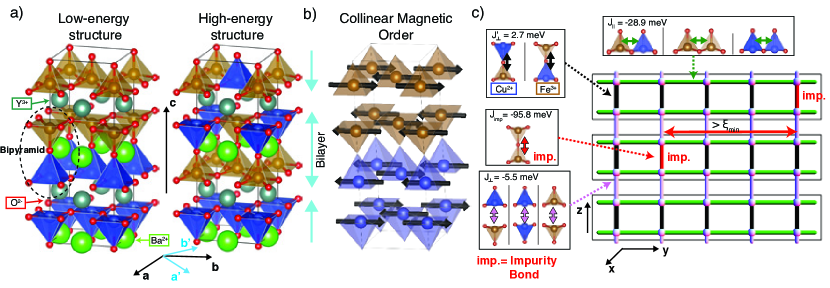
Figure 1: (a) Two different orderings of Cu²⁺ and Fe³⁺ in the $\sqrt{2}\times\sqrt{2}\times 2$ supercell of YBaCuFeO₅. The FeO₅ and the CuO₅ square pyramids are shown in gold and blue, respectively. The left panel shows a low-energy structure consisting only of Fe³⁺–Cu²⁺ bipyramids. The right panel shows a high-energy structure with one Fe³⁺-Fe³⁺ and, upon periodic repetition, one Cu²⁺-Cu²⁺ bipyramid. (b) Unfrustrated magnetic order in the commensurate phase. (c) Simplified spin model for YBaCuFeO₅ with nearest-neighbor exchange interactions. The $a^{\prime}$- and $b^{\prime}$-axes are rotated by 45^∘ with respect to the $a$- and $b$-axes in (a). The magnetic ions are depicted as pink spheres. They correspond to either Cu²⁺ or Fe³⁺. They form stacked bilayers (regions enclosed by the rectangles) obtained by stacking a pair of $x$–$y$ square lattices (corresponding to YBaCuFeO₅ bilayers) along the $z$ axis. The antiferromagnetic exchange coupling $J^{\,}_{\parallel}$ within a layer is assumed to be independent of whether it couples Fe³⁺ with Fe³⁺, Cu²⁺ with Cu²⁺ or Fe³⁺ with Cu²⁺. The inter-layer coupling $J^{\prime}_{\perp}$ within a bilayer is ferromagnetic for Cu²⁺-Fe³⁺ bipyramids (see text). Impurity bonds have a strong antiferromagnetic exchange, $J^{\,}_{\mathrm{imp}}$, similar in magnitude to the ab initio value for Fe³⁺-Fe³⁺ bipyramids. The impurity bonds are randomly distributed, up to the constraint that two impurity bonds in adjacent bilayers cannot be closer than a minimal distance $\xi^{\,}_{\mathrm{min}}$.

A recent ab initio study Morin et al. (2015) revealed that the lowest energy arrangements of Fe and Cu ions contain only Fe³⁺–Cu²⁺ bipyramids as shown in the left panel of Fig. 1(a). The exchange interactions between the magnetic ions making up these low-energy structures were also calculated using LSDA+U. The exchange interactions within the Fe-Cu bipyramids were found to be uniform in sign (ferromagnetic), and so unfrustrated, and thus cannot explain the emergence of a magnetic spiral. Bipyramids of Cu²⁺–Cu²⁺ and Fe³⁺–Fe³⁺, shown in the right panel of Fig. 1(a), are energetically more costly, but they nevertheless occur as local defects that form during preparation and thermal treatment of the sample. The Fe³⁺–Fe³⁺ bipyramids introduce strongly frustrating antiferromagnetic couplings along the $c$ axis . In the following, we show that a small concentration of Fe³⁺-Fe³⁺ bipyramids is at the microscopic origin of the spiral order.

We model the magnetic ordering of YBaCuFeO₅ using the classical Hamiltonian

$$H=-\frac{1}{2}\sum_{\boldsymbol{r},\boldsymbol{r}^{\prime}}J^{\,}_{\boldsymbol{r},\boldsymbol{r}^{\prime}}\,\boldsymbol{S}^{\,}_{\boldsymbol{r}}\cdot\boldsymbol{S}^{\,}_{\boldsymbol{r}^{\prime}}+\frac{\Delta}{2}\sum_{\boldsymbol{r}}(\boldsymbol{S}^{\,}_{\boldsymbol{r}}\cdot\hat{\boldsymbol{n}})^{2}.$$ (1)

Here, the classical spin $\boldsymbol{S}_{\boldsymbol{r}}$ is a three-component unit vector located at the site $\boldsymbol{r}$ of a cubic lattice isomorphic to the tetragonal lattice of YBaCuFeO₅. To distinguish between the lattice vectors of the real material and those of the spin model we label the latter as $\boldsymbol{x}$, $\boldsymbol{y}$, and $\boldsymbol{z}$. Their length is equal to $a_{\,}^{\prime}=b_{\,}^{\prime}\approx c/2$ where $\boldsymbol{a}^{\prime}_{\,}$, $\boldsymbol{b}^{\prime}_{\,}$, and $\boldsymbol{c}$ are the lattice vectors of YBaCuFeO₅ as shown in Fig. 1 (with $\boldsymbol{c}\parallel\boldsymbol{z}$). To facilitate comparison with experiments, we express the wave vectors in units of the reciprocal vectors of the crystallographic unit cell of YBaFeCuO₅ throughout. We retain only nearest-neighbor exchange interactions. The $ab$ planes host spins on a square lattice, coupled antiferromagnetically with the strong exchange $J^{\,}_{\parallel}=-28.9\,\mathrm{meV}$  . These planes are stacked along the $c$ axis in bilayers (Fig. 1). Within a bilayer, the nearest neighbors along the $c$ axis, that is the spins in a bipyramid, are coupled with the weak ferromagnetic exchange interaction $J^{\prime}_{\perp}=2.7\,\mathrm{meV}>0$. Adjacent bilayers are coupled with the relatively weak antiferromagnetic coupling $J^{\,}_{\perp}=-5.5\,\mathrm{meV}$. Finally, the defect bipyramids are modelled by a small concentration, $n^{\,}_{\mathrm{imp}}$, of randomly located “impurity bonds” lying within the bilayers. They substitute $J^{\prime}_{\perp}>0$ with the strong antiferromagnetic coupling $J^{\,}_{\text{imp}}=-95.8\,\mathrm{meV}$ calculated for Fe³⁺–Fe³⁺ bipyramids and locally frustrate the ferromagnetic intra-bilayer couplings inducing a local canting for $|J^{\,}_{\text{imp}}|$ sufficiently larger than $J^{\,}_{\parallel}$. At the same time, we assume impurities to be sufficiently dilute, ($n^{\,}_{\mathrm{imp}}\,J^{\,}_{\mathrm{imp}}\lesssim J^{\prime}_{\perp}$), so that intralayer antiferromagnetic alignment does not become favored within bilayers. The impurity bonds are long-range correlated in the sense that they are always oriented parallel to the $c$ axis. We do not include the Cu²⁺–Cu²⁺ bipyramids (which stoichiometry implies to be as abundant as the Fe³⁺-Fe³⁺ bipyramids) since their inter-layer exchange is substantially smaller than all other couplings.

The second term in Eq. (1) describes a small easy plane anisotropy with $\Delta=0.5$ meV which favors magnetic moments in the plane perpendicular to the direction defined by the unit vector $\hat{\boldsymbol{n}}$. The spiral order parameter is defined by

$$P=\frac{1}{N}\sum_{\boldsymbol{r}}(\mathbf{S}^{\,}_{\boldsymbol{r}}\wedge\mathbf{S}^{\,}_{\boldsymbol{r}+\boldsymbol{z}})\cdot\hat{\boldsymbol{n}},$$ (2)

where $N$ is the number of spins in the lattice. Neutron scattering shows that $\hat{\boldsymbol{n}}\neq\hat{\boldsymbol{c}}$, which ensures a cycloidal component of the spiral and thus a coupling to the electric polarization . For the calculation of the thermodynamics, the orientation of $\hat{\boldsymbol{n}}$ plays no role.

In our Monte Carlo simulations, we use a cubic superlattice of linear dimension $L\times L\times 2L$ (where $L\leq 28$) with periodic boundary conditions in plane and open boundary conditions in the $\boldsymbol{z}$ direction. Impurity bonds are randomly located, but subject to the constraint that any two impurity bonds in adjacent bilayers are further apart than a cutoff in-plane distance $\xi_{\mathrm{min}}$ (tuned to be $2.5$ or $4$ in units of the lattice spacing). This cutoff embodies the main effect of the strong Coulomb repulsion between Fe³⁺–Fe³⁺ bipyramids. We consider small impurity bond concentrations $n_{\mathrm{imp}}~{}\leq 0.04\sim J^{\prime}_{\perp}/|J^{\,}_{\mathrm{imp}}|$ per unit cell. Monte Carlo results include a disorder averaging over 16 configurations of the impurity bonds. A more complete description of the model, the method and detailed Monte Carlo data including system-size dependence are given in the supplemental material Sup .

For the clean, unfrustrated case ($n_{\mathrm{imp}}=0$), we find a transition at $T^{\,}_{\mathrm{N}}\simeq 300$ K $=O(J^{\,}_{\parallel})$ from the high-temperature paramagnetic phase to a low-temperature collinear antiferromagnetic phase with the ordering wave vector $(\frac{1}{2},\frac{1}{2},\frac{1}{2})$. This is consistent with the antiferromagnetic ordering observed experimentally at high temperature in Ref. Morin et al. (2015) and shown in Fig. 1(b). The calculated specific heat $C$ at constant volume is shown in the first panel of Fig. 2(a). It shows a typical $\lambda$-peak at $T^{\,}_{\mathrm{N}}$, characteristic of a continuous transition.

With a finite concentration of impurity bonds, $n_{\mathrm{imp}}>0$, the peak in $C$ broadens, while its position remains almost constant as long as $n_{\mathrm{imp}}\leq 0.04$. However, the magnitude of the collinear order parameter, $m_{\mathrm{AF}}$, shown in the second panel of Fig. 2(a), is strongly suppressed below $T=T^{\,}_{\mathrm{spi}}\simeq 150$ K for $n^{\,}_{\mathrm{imp}}=0.02$. This fact suggests the onset of spiral order. Simultaneously, the electric polarization (estimated as $\sqrt{\langle P^{2}\rangle}$) becomes non-zero. The associated susceptibility $\chi^{\,}_{P}$ exhibits a peak, which seems to diverge as the system size increases, as shown in the supplemental material Sup . In Fig. 2(b), we show the spin-structure factor $S(q^{\,}_{c})$ as a function of the wave vector $q^{\,}_{c}$ along the $c$ axis (averaged over $q^{\,}_{a}$ and $q^{\,}_{b}$) and temperature, for four values of $n_{\mathrm{imp}}$. At $n_{\mathrm{imp}}=0.02$, the propagation wave vector $q^{\,}_{c}$ of the magnetic order decreases smoothly from $\pi$ below $T_{\mathrm{spi}}$, suggesting a continuous transition from the antiferromagnetic phase to a spiral-ordered phase, consistent with the experimental observations reported in Ref. Morin et al. (2015). A small residual $m_{\mathrm{AF}}$ below $T_{\mathrm{spi}}$ remains. This might be due to either finite-size effects or to a coexistence of the spiral and antiferromagnetic order Sup . Figure 2(c) shows $T^{\,}_{\mathrm{spi}}$, estimated from the peak of $\chi^{\,}_{P}$ (see Supplemental Material), as a function of impurity concentration. At large impurity concentration, $n_{\rm imp}\gtrsim 0.04$, a direct transition from the paramagnet to an incommensurate spiral state with $q_{\rm spi}<1/2$ is also compatible with the finite resolution of our data.

We carried out Monte Carlo simulations for two values of the minimal in-plane distance between impurity bonds $\xi_{\mathrm{min}}=2.5$ and $\xi_{\mathrm{min}}=4$ for each value of $n^{\,}_{\mathrm{imp}}$. As $n_{\mathrm{imp}}$ increases, $T^{\,}_{\mathrm{spi}}$ increases and almost reaches $T^{\,}_{\mathrm{N}}$ (as estimated from the peak in specific heat) at $n_{\mathrm{imp}}=0.04$. Note that at $n_{\mathrm{imp}}=0.04$, $S(q^{\,}_{c})$ has a maximum at $q^{\,}_{c}~{}<\pi$ even at high temperature. This behavior does not rule out a direct transition from the paramagnetic to the spiral phase for larger (but not too large) values of $n_{\mathrm{imp}}$. Note that our values of $T^{\,}_{\mathrm{spi}}$ constitute lower bounds due to finite size effects in the Monte Carlo simulations. Indeed, the peak values for $\chi^{\,}_{P}$ are still moving to higher temperatures for the largest linear system sizes $L$ that were used in the Monte Carlo simulations. Hence, the finite size effects on $T^{\,}_{\mathrm{spi}}$ are expected to be sizable for the values of $L$ used in our Monte Carlo simulations.

Finally, we discuss the short range repulsion among the impurity bonds, which we model by imposing $\xi_{\mathrm{min}}$. We find that when we neglect to include this effect, by setting $\xi_{\mathrm{min}}=0$, the low temperature state does not support any spiral order over the range $0.02\leq n_{\mathrm{imp}}\leq 0.04$ that we studied. Instead, a “fan state” in which the intralayer ferromagnetic order oscillates is stabilized, as shown in panel (c) of Fig. 4; this state will be discussed in more detail elswehere Scaramucci et al. (2016). Comparing the phase diagrams obtained for $\xi_{\mathrm{min}}=4$ and $\xi_{\mathrm{min}}=2.5$ in Fig. 2, we see that $T_{\mathrm{spi}}$ decreases with decreasing $\xi_{\mathrm{min}}$. Indeed, the spiral order is favored if the presence of impurity bonds is suppressed in directions forming small angles with the $c$ axis, where the coupling has antiferromagnetic sign.

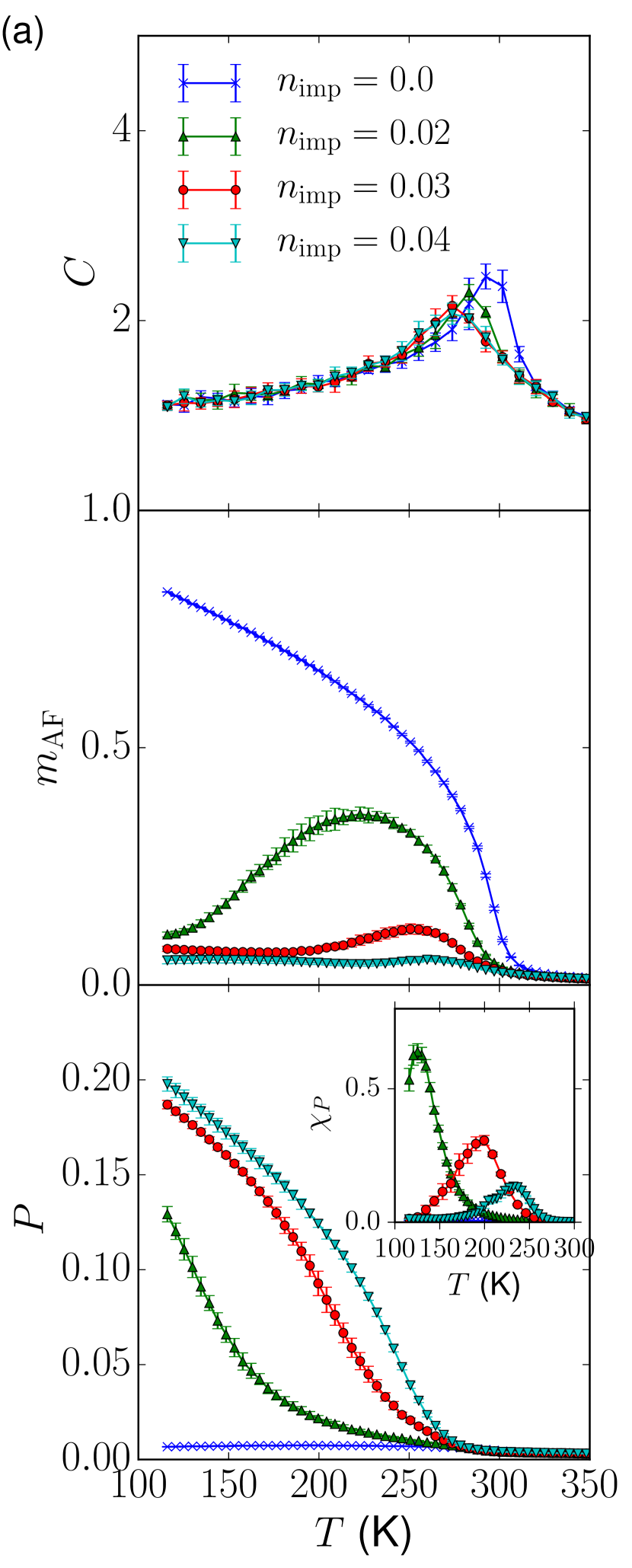
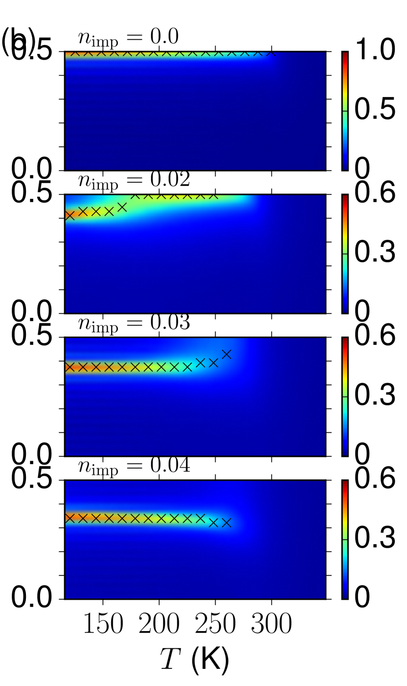
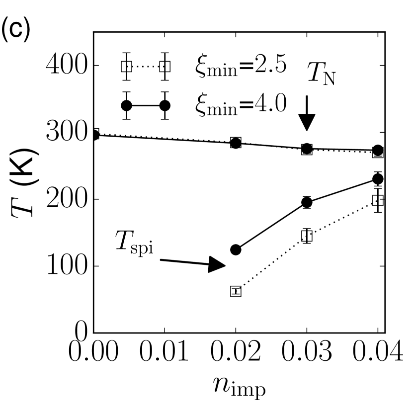
Figure 2: Monte Carlo results obtained for systems of size $L=28$. (a) Specific heat $C$, collinear antiferromagnetic order parameter $m_{\mathrm{AF}}$ and polarization $P$, which we estimated by computing $\sqrt{\langle P^{2}\rangle}$, for $\xi_{\mathrm{min}}=4$ and a range of impurity bond concentrations. (b) Square root of the spin-structure factor $S(q^{\,}_{c})$ computed for $\xi_{\mathrm{min}}=4$. The data are averaged over the in-plane wave vectors. The crosses represent the wave vector where $S(q_{c})$ takes a maximum value at the given temperature. The data for $n_{\rm imp}=0.04$ is compatible with a direct transition from the paramagnetic state into an incommensurate magnetic state with $q_{\mathrm{spi}}<1/2$. (c) Phase diagrams obtained for $\xi_{\mathrm{min}}=2.5$ and $\xi_{\mathrm{min}}=4$.

In summary, our simulations reveal that in the range $0.02\leq n_{\mathrm{imp}}\leq 0.04$ the low temperature state is a spiral with a temperature-dependent wave vector provided the impurity bonds obey the condition that $\xi_{\mathrm{min}}\gtrsim 2.5$. Both the spiral ordering temperature $T^{\,}_{\text{spi}}$ and the component $1/2-\boldsymbol{q}^{\,}_{\mathrm{spi}}\cdot\hat{\boldsymbol{c}}$ of the ordering wave vector depend on the concentration $n^{\,}_{\mathrm{imp}}$ of the impurity bonds and are proportional to the latter in the limit of small $n^{\,}_{\mathrm{imp}}$.

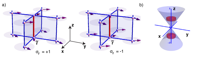
Figure 3: (a) Sketch of the two ground states of Hamiltonian (1) for a single bilayer, in the presence of a single frustrating impurity bond (red line). For visualization purposes the spins on every other site in the $ab$-plane have been reversed so that the unfrustrated ground state looks ferromagnetic. The two ground states break the local inversion symmetry and correspond to counter-clockwise (left panel) and clockwise (right panel) rotation of the spins as one proceeds along the $c$ axis. They can be labeled by an Ising variable $\sigma^{\,}_{\tilde{\boldsymbol{r}}}$. Spin waves mediate an effective interaction $\Gamma^{\,}_{\tilde{\boldsymbol{r}},\tilde{\boldsymbol{r}}^{\prime}}$ between the local orientations $\sigma^{\,}_{\tilde{\boldsymbol{r}}}$ and $\sigma^{\,}_{\tilde{\boldsymbol{r}}^{\prime}}$ of the cantings around two impurity bonds $\langle\tilde{\boldsymbol{r}},\tilde{\boldsymbol{r}}+\boldsymbol{z}\rangle$ and $\langle\tilde{\boldsymbol{r}}^{\prime},\tilde{\boldsymbol{r}}^{\prime}+\boldsymbol{z}\rangle$, as given by Eq. (3). (b) The blue cone is the domain of $\Delta\tilde{\boldsymbol{r}}=\tilde{\boldsymbol{r}}-\tilde{\boldsymbol{r}}^{\prime}$ for which the effective interaction $\Gamma^{\,}_{\tilde{\boldsymbol{r}},\tilde{\boldsymbol{r}}^{\prime}}$ is antiferromagnetic, while outside it is ferromagnetic. The short range constraint $\xi^{\,}_{\mathrm{min}}$ excludes the domains represented by the red cylinders and thus increases the probability of a ferromagnetic coupling between neighboring Ising variables.

Mechanism for spiral stabilization – Finally, we analyze the limit of low concentration of impurity bonds $n^{\,}_{\mathrm{imp}}$ and low temperature $T$, to provide insight into the mechanism for stabilization of the spiral. As discussed in detail in Ref. Scaramucci et al. (2016), impurity bonds induce cantings which are coupled through the spin stiffnes of the hosting spin lattice. For systems with continuous symmetry such effective coupling is dipolar and analogous to the Coulomb coupling that occurs for vortices in the two dimensional $XY$ model. Moreover, the net value of dipoles couples linearly to the winding of the spins of the hosting lattice along the $z$ axis. Therefore, distributions of impurity bonds having a ground state with a non-vanishing net dipole stabilize a spin spiral. At $T\ll\Delta$, the spins become coplanar $XY$ spins with $\boldsymbol{S}\cdot\hat{\boldsymbol{n}}=0$. For $n^{\,}_{\mathrm{imp}}=0$, the antiferromagnetic ground state has all spins parallel in the $xy$-plane, e.g., parallel to the $x$ axis. A single impurity bond with exchange of magnitude $|J^{\,}_{\mathrm{imp}}|$ above a threshold value $J^{\,}_{\mathrm{c}}$ (where $J^{\,}_{\mathrm{c}}\approx J^{\,}_{\parallel}/[C-\ln(J^{\prime}_{\perp}/J^{\,}_{\parallel})/(2\pi)]$ with $C\sim 0.4$ for $J^{\prime}_{\perp}/J^{\,}_{\parallel}\ll 1$) renders the ground state two-fold degenerate, see Fig. 3. Far away from the impurity bond, the staggered magnetization parallel to the $x$ axis is restored. Close to the impurity bond, the coplanar spins are canted away from the $x$ axis with the two ground states differing in the local sense of rotation of spins, as given by $P^{\,}_{\mathrm{loc}}(\tilde{\boldsymbol{r}})=\left(\mathbf{S}^{\,}_{\tilde{\boldsymbol{r}}}\wedge\mathbf{S}^{\,}_{\tilde{\boldsymbol{r}}+\hat{\boldsymbol{z}}}\right)\cdot\hat{\boldsymbol{n}}$. At finite but small $n^{\,}_{\mathrm{imp}}>0$ the impurity bonds are well separated. Thus, the low energy configurations can be labelled by local Ising variables $\sigma^{\,}_{\tilde{\boldsymbol{r}}}=\mathrm{sgn}\,P^{\,}_{\mathrm{loc}}(\tilde{\boldsymbol{r}})$ describing the sign of the local cantings, while the remaining degrees of freedom are well captured by spin waves. Integrating them out yields an effective Hamiltonian $H^{\,}_{\mathrm{eff}}$ for the Ising degrees of freedom

$$H^{\,}_{\mathrm{eff}}=-\frac{\alpha^{2}}{2}\,\left(\sum_{\tilde{\boldsymbol{r}},\tilde{\boldsymbol{r}}^{\prime}\in\mathcal{L}}\Gamma^{\,}_{\tilde{\boldsymbol{r}},\tilde{\boldsymbol{r}}^{\prime}}\,\sigma^{\,}_{\tilde{\boldsymbol{r}}}\,\sigma^{\,}_{\tilde{\boldsymbol{r}}^{\prime}}+\frac{N\,|J^{\,}_{\perp}|}{\alpha^{2}}\,Q^{2}\right),$$ (3a)

for a system with $$N |J^{\,}_{\perp}|=J^{\prime}_{\perp} \tilde{\boldsymbol{r}} \mathcal{L} Q$$ lattice sites, where we simplified the model slightly by setting . We label the impurity bonds by the site at their lower end and by the ensemble of such sites for a given distribution of impurity bonds. Here, is the saddle-point value of the spiral wave vector and is proportional to the net value of the Ising spins,

$$Q=-\frac{|\alpha|}{N\,|J^{\,}_{\perp}|}\sum_{\tilde{\boldsymbol{r}}\in\mathcal{L}}\sigma^{\,}_{\tilde{\boldsymbol{r}}}.$$ (3b)

It is non-zero provided the ground state of the effective Ising model has a net magnetization. In Eq. (3a), $$\alpha=(|J^{\,}_{\mathrm{imp}}|+|J^{\,}_{\parallel}|)\,|P^{\mathrm{imp}}_{\mathrm{loc}}| P^{\mathrm{imp}}_{\mathrm{loc}} \Gamma$$ where encodes the canting angle at an isolated impurity bond Scaramucci et al. (2016). As shown in Ref. Scaramucci et al. (2016), at large distances the kernel takes the (anti-) dipolar form

$$\Gamma^{\,}_{\tilde{\boldsymbol{r}},\tilde{\boldsymbol{r}}^{\prime}}\sim\frac{\sqrt{|J^{\,}_{\parallel}|}}{4\pi}\frac{|J^{\,}_{\perp}|\left(\Delta\tilde{r}^{2}_{x}+\Delta\tilde{r}^{2}_{y}\right)-2|J^{\,}_{\parallel}|\,\Delta\tilde{r}^{2}_{z}}{\left[|J^{\,}_{\perp}|\left(\Delta\tilde{r}^{2}_{x}+\Delta\tilde{r}^{2}_{y}\right)+|J^{\,}_{\parallel}|\,\Delta\tilde{r}^{2}_{z}\right]^{\frac{5}{2}}}.$$ (3c)

Note that $\Gamma^{\,}_{\tilde{\boldsymbol{r}},\tilde{\boldsymbol{r}}^{\prime}}$ is ferromagnetic if $\Delta\tilde{r}^{2}_{x}+\Delta\tilde{r}^{2}_{y}>\sqrt{2}|J^{\,}_{\parallel}|\,\Delta\tilde{r}^{2}_{z}/|J^{\,}_{\perp}|$ and antiferromagnetic otherwise, as illustrated in Fig. 3(b). In particular, the ratio of the in-plane nearest-neighbor interaction to the inter-plane one scales like $(J^{\,}_{\parallel}/J^{\,}_{\perp})^{3/2}\gg 1$. We thus expect ferromagnetic order in-plane. The inter-layer order might be either ferromagnetic or antiferromagnetic. Now, the Coulomb repulsion between Fe³⁺/Fe³⁺ bipyramids amounts to a suppression of antiferromagnetically coupled pairs of nearest-neighbor impurities. A mean-field calculation shows that this constraint stabilizes ferromagnetic inter-layer order. In the numerical simulation, we retain the essential part of the short-distance repulsion by forbidding impurity bonds on adjacent bilayers to be closer than $\xi^{\,}_{\mathrm{min}}$ in plane. Increasing $\xi^{\,}_{\mathrm{min}}$ indeed enhances the tendency toward a ferromagnetic Ising ground state with a finite $Q=n^{\,}_{\rm imp}|\alpha/J_{\perp}|$ (as opposed to competing inter-layer antiferromagnetic order, which has vanishing $Q$).

The latter immediately translates into a spiral order of the spins $\boldsymbol{S}^{\,}_{\boldsymbol{r}}$, with the characteristic wave vector $\boldsymbol{q}^{\,}_{\mathrm{spi}}=(\frac{1}{2},\frac{1}{2},\frac{1}{2}-Q)$. The linear dependence of $Q$ on $n^{\,}_{\mathrm{imp}}$ is in qualitative agreement with the $n^{\,}_{\mathrm{imp}}$-dependence of the peak of the low $T$ structure factor, as calculated with Monte Carlo simulations and presented in Fig. 2 (b).

The ground state of the effective Ising Hamiltonian (3) can be solved analytically when the set of impurity bonds forms a superlattice. Following Ref. Scaramucci et al. (2016), we assume that the impurity bonds form a Bravais lattice with the basis $\boldsymbol{A}$, $\boldsymbol{B}$, and $\boldsymbol{C}$ , such that $n^{\,}_{\mathrm{imp}}=\frac{\boldsymbol{a}\cdot(\boldsymbol{b}\wedge\boldsymbol{c})}{\boldsymbol{A}\cdot(\boldsymbol{B}\wedge\boldsymbol{C})}\ll 1$. In Figs. 4(a) and 4(b) we compare the ground state of Eq. (3a) with the ground state obtained by Monte Carlo simulations of Eq. (1). For both calculations we take $|J^{\prime}_{\perp}|=|J^{\,}_{\perp}|=4.1$ meV to be the average of the actual $|J^{\,}_{\perp}|$ and $|J^{\prime}_{\perp}|$ given in Fig. 1. In agreement with the magnetic structure obtained by the refined analysis of the elastic neutron scattering data, the obtained magnetic spiral has the feature that the rotation of magnetic moments mainly happens between neighboring $ab$-layers coupled by impurity bonds (e.g., bilayers of the YBaCuFeO₅ structure).

Fig. 4(c) is a similar comparison, but for a superlattice favoring a state with no net winding of the spins, i.e., a fan-like magnetic state.

Finally, Fig. 4(d) shows the concentration dependence of the polarization $P$ (see Eq. 2) calculated both numerically from Eq. (1) and using the effective Ising Hamiltonian (3) for various superlattices for which the ground state is a spiral. The values of polarization predicted by the effective model match well the values of polarization obtained numerically for the ground state of a finite system. Furthermore, the value of $P$ increases proportionally to $n_{\mathrm{imp}}$ for small values of $P$ as predicted by the effective model.

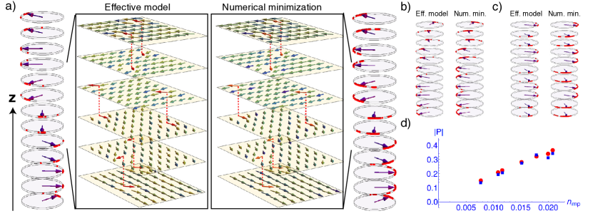
Figure 4: (a) Comparison of a spiral ground state corresponding to an Ising ferromagnetic ground state of the effective Ising Hamiltonian (3a) (left) against the spiral ground state of the Heisenberg Hamiltonian (1) (right). The violet arrows represent the average directions of the staggered magnetization for each layer. The red dots lying on the circle represent the direction of each spin in a given plane. The staggered magnetization of layers corresponding to even bilayers have been reversed for visualization purposes. The two central panels depict the ground states in a portion of six layers of the lattice of overall dimensions $14\times 14\times 32$. Here, the color of the arrows indicate the angular difference of each spin from the average staggered magnetization of the layer and the vertical red lines depict the impurity bonds. For visualization purposes, spins at every other sites in the $ab$ plane and at every other bilayer have been reversed. The results were obtained for a superlattice of impurity bonds with lattice constants $\boldsymbol{A}=(4,3,0)$, $\boldsymbol{B}=(0,4,2)$, and $\boldsymbol{C}=(4,0,2)$. The values of the couplings are $J^{\,}_{\parallel}=28.9$ meV , $J^{\,}_{\perp}=J^{\prime}_{\perp}=4.1$ meV and $J^{\,}_{\mathrm{imp}}=-95.8$ meV. (b) Comparison of the spiral ground state obtained using the effective Ising Hamiltonian (3a) (left) against the spiral ground state of the Heisenberg Hamiltonian (1) (right) for the same value of the couplings but with $\boldsymbol{A}=(5,3,2)$, $\boldsymbol{B}=(3,0,4)$, and $\boldsymbol{C}=(2,4,6)$. Panel (c) shows the same comparison for the choice: $\boldsymbol{A}=(5,0,0)$, $\boldsymbol{B}=(0,5,0)$, and $\boldsymbol{C}=(0,1,2)$. For such a superlattice of impurity bonds a “fan state” (with no net winding along the $c$ axis) is stabilized instead of a spiral (d) Concentration dependence of the magnitude of $P$ defined in Eq. (2) for the ground states obtained from the effective Ising Hamiltonian (3a) (red dots) and the Heisenberg Hamiltonian (1) (right) (blue squares) for various superlattices of impurity bonds stabilizing a spiral state.

Conclusions. We have presented a mechanism in which impurity bonds, when sufficiently strong, induce a local frustration in an otherwise non-frustrated lattice of classical spins. The associated cantings become long-range correlated at low temperature, resulting in a spiral magnetic order in which the sense of rotation of the spiral is spontaneously chosen. The spiral formation is in contrast to the spin-glass phase expected for white-noise correlated random magnetic exchange interactions Edwards and Anderson (1975); Villain (1975, 1977, 1978); Binder and Young (1986), and is caused by orientational long-range correlations, which align the impurity bonds along one crystallographic direction of the lattice. The critical temperature below which the spiral order develops is controlled by nearest-neighbor exchange couplings, which can be sizable, so the mechanism is relevant for engineering high temperature multiferroics.

When the model is applied to YBaCuFeO₅ with realistic couplings, it predicts a multiferroic phase that is consistent with several distinct features observed experimentally. (i) It captures the transition to a commensurate antiferromagnet phase with wave vector $\boldsymbol{q}^{\,}_{\mathrm{N}}\equiv(\frac{1}{2},\frac{1}{2},\frac{1}{2})$ at the Néel temperature $T^{\,}_{\mathrm{N}}$, followed by a transition to an incommensurate spiral phase with wave vector $\boldsymbol{q}^{\,}_{\mathrm{spi}}\equiv(\frac{1}{2},\frac{1}{2},\frac{1}{2}-Q)$ at the lower critical temperature $T^{\,}_{\mathrm{spi}}$. (ii) It gives rise to a magnetic spiral phase, in which the rotation of the magnetic moments neighboring along $c$ occurs mainly when they belong to the same bilayer. (iii) The observed temperature dependence of $Q$ in YBaCuFeO₅ is well reproduced. (iv) Finally, the dependence of both $T^{\,}_{\mathrm{spi}}$ and $\boldsymbol{q}^{\,}_{\mathrm{spi}}$ on the concentration $n^{\,}_{\rm imp}$ is in qualitative agreement with the dependence on the annealing conditions of the YBaCuFeO₅ samples: The faster the quench ( and thus the higher the expected defect concentration), the larger the measured $T^{\,}_{\mathrm{spi}}$ and $\boldsymbol{q}^{\,}_{\mathrm{spi}}$.

We close by mentioning other compounds with magnetic spiral order whose origin is not understood so far, but to which the mechanism presented in this paper might apply. For solid solutions of Cr₂O₃ and Fe₂O₃ Cox et al. (1963) and for the doped hexaferrite Ba_(1-x)Sr_xZn₂Fe₁₂O₂₂ Utsumi et al. (2007), the wave vector of the spiral order is known to change smoothly from a commensurate value at high temperature to an incommensurate value at low temperature. In all cases, the maximal value of the concentration dependent $T^{\,}_{\mathrm{spi}}$ is high ($T^{\mathrm{max}}_{\mathrm{spi}}=148$ K for solid solutions of Cr₂O₃ and Fe₂O₃Cox et al. (1963) and $T^{\mathrm{max}}_{\mathrm{spi}}$ higher than $294$ K for Ba_(1-x)Sr_xZn₂Fe₁₂O₂₂ Momozawa et al. (1985)). Moreover, the wave vector and the transition temperature to the spiral state are dependent on the dopant concentration. Since in both compounds cation substitution can introduce impurity bonds, they are likely candidates to realize “spiral order by disorder”.

I Acknowledgments

This research was partially supported by NCCR MARVEL, funded by the Swiss National Science Foundation. H.S. acknowledges support from the DFG via FOR 1346, the SNF Grant 200021E-149122, ERC Advanced Grant SIMCOFE, ERC Consolidator Grant CORRELMAT (project number 617196). Computer time was provided through a grant from the Swiss National Supercomputing Centre (CSCS) under project ID p504 as well as by the Brutus cluster of ETH Zürich. We thank M. Kenzelmann, M. Medarde and M. Morin for very useful discussions.

Supplemental Materials: Multiferroic magnetic spirals induced by random magnetic exchanges

II Monte Carlo (MC) simulation

We model the magnetic properties of YBaCuFeO₅ (YBCF) as follows. We use the crystallographic unit cell labelled by the vector $\boldsymbol{r}\in\mathbb{R}^{3}$ and comprising two magnetic ions aligned along the $\boldsymbol{c}$ direction and belonging to the same bilayer. Therefore, in what follows, the position of each unit cell is defined by

$$\boldsymbol{r}:=m\,\boldsymbol{a}^{\prime}+n\,\boldsymbol{b}^{\prime}+2l\,\boldsymbol{c}$$ (S1a)

where $$m,n,l\in\mathbb{Z} \boldsymbol{a}^{\prime} \boldsymbol{b}^{\prime} 2\boldsymbol{c} \mu=1,2 \boldsymbol{S}^{\,}_{\mu,\boldsymbol{r}} \mathbb{R}^{3} \Delta>0$$ and , , and is a basis for the crystallographic lattice vectors. We distinguish the two inequivalent magnetic sublattices with the index . As described in the main text, the classical spins are unit vectors in and a single-ion easy-plane anisotropy with the characteristic energy scale is included. All together, the classical Hamiltonian [Eq. (1) in the main text] is

$$H^{\,}_{\mathcal{L}}:=-\frac{1}{2}\sum_{\begin{subarray}{c}\boldsymbol{r},\boldsymbol{r}^{\prime}\\ \mu,\nu=1,2\end{subarray}}J^{\mu,\nu}_{\boldsymbol{r},\boldsymbol{r}^{\prime}}\,\boldsymbol{S}^{\,}_{\boldsymbol{r},\mu}\cdot\boldsymbol{S}^{\,}_{\boldsymbol{r}^{\prime},\nu}+H^{\,}_{\mathrm{imp}}+\frac{\Delta}{2}\sum_{\begin{subarray}{c}\boldsymbol{r}\\ \mu=1,2\end{subarray}}\left(S^{c}_{\boldsymbol{r},\mu}\right)^{2}.$$ (S1b)

There are three characteristic energy scales. The antiferromagnetic in-plane exchange coupling $$J^{\,}_{\parallel}\leq 0 \boldsymbol{c} J^{\prime}_{\perp}\geq 0 J^{\,}_{\perp}\leq 0 \boldsymbol{c}$$, the intra-unit cell (intra-layer along the direction) ferromagnetic exchange coupling , and the inter-unit cell (inter-layer) antiferromagnetic exchange coupling (also along the direction). They enter Eq. (S1b) according to the rules,

$$J^{1,2}_{\boldsymbol{r},\boldsymbol{r}^{\prime}}\>=J^{\prime}_{\perp}\,\delta^{\,}_{\boldsymbol{r},\boldsymbol{r}^{\prime}}+J^{\,}_{\perp}\delta^{\,}_{\boldsymbol{r},\boldsymbol{r}^{\prime}+2\boldsymbol{c}},$$ (S1c)

$$J^{2,1}_{\boldsymbol{r},\boldsymbol{r}^{\prime}}\>=J^{\prime}_{\perp}\,\delta^{\,}_{\boldsymbol{r},\boldsymbol{r}^{\prime}}+J^{\,}_{\perp}\delta^{\,}_{\boldsymbol{r},\boldsymbol{r}^{\prime}-2\boldsymbol{c}},$$ (S1d)

$$J^{1,1}_{\boldsymbol{r},\boldsymbol{r}^{\prime}}=J^{2,2}_{\boldsymbol{r},\boldsymbol{r}^{\prime}}\>=J^{\,}_{\parallel}\sum_{\boldsymbol{\alpha}=\pm\boldsymbol{a^{\prime}},\pm\boldsymbol{b^{\prime}}}\,\delta^{\,}_{\boldsymbol{r},\boldsymbol{r}^{\prime}+\boldsymbol{\alpha}}.$$ (S1e)

The subscript $$\mathcal{L} \mathcal{L}$$ for the Hamiltonian (S1b) indicates its dependence on the choice made for the set of impurity bonds. This dependence arises from the term

$$H^{\,}_{\mathrm{imp}}\>=\left(|J^{\,}_{\mathrm{imp}}|+J^{\prime}_{\perp}\right)\sum_{\tilde{\boldsymbol{r}}\in\mathcal{L}}\boldsymbol{S}^{\,}_{\tilde{\boldsymbol{r}},1}\cdot\boldsymbol{S}^{\,}_{\tilde{\boldsymbol{r}},2},$$ (S1f)

which substitutes any ferromagnetic intra-layer bond associated with the exchange coupling $J^{\prime}_{\perp}\geq 0$ belonging to $\mathcal{L}$ with an antiferromagnetic impurity bond associated with the exchange coupling $J^{\,}_{\mathrm{imp}}\leq 0$. In the cell considered for the Monte Carlo simulations, there are $L\times L\times L$ crystallographic unit cells, i.e., the cell contains $N=2L^{3}$ spins. The values of the exchange couplings are those given in the main text ($J^{\,}_{||}=-28.9$ meV, $J^{\,}_{\perp}=-5.5$ meV, $J^{\prime}_{\perp}=2.7$ meV, $J^{\,}_{\mathrm{imp}}=-95.8$ meV and $\Delta=0.5$ meV).

We employ the exchange Monte Carlo Hukushima and Nemoto (1996) and overrelaxation Alonso et al. (1996) method using 200 temperature ($T$) points in the range of $10\leq k^{\,}_{\mathrm{B}}T\leq 30$ (meV^-1) for $L=28$. Replicas are exchanged between two neighbouring temperatures. The distribution of the temperatures is optimized so that the exchange rate is independent of $T$. Thermodynamic observables are measured using the reweighting method Landau and Binder (2001). Periodic boundary conditions in the $ab$ plane and open boundary conditions along the $c$ direction are used in order to deal with a magnetic spiral order with an incommensurate wave vector.

Monte Carlo simulations are performed for several sets $\mathcal{L}$ chosen randomly. As described in the main text, the randomly chosen impurity bonds satisfy the constraint that there be a minimal lateral distance $\xi_{\mathrm{min}}$ between impurity bonds separated by $2c$ along the $\boldsymbol{c}$ axis of the pseudocubic lattice. We denote with $\langle\cdots\rangle^{\,}_{\mathrm{MC}}$ the Monte Carlo average and with $\langle\cdots\rangle^{\,}_{\mathcal{L}}$ the average over randomly chosen sets $\mathcal{L}$. Denoting with Eq. (S1a) the position of the unit cell, we define the collinear antiferromagnetic order parameter $m_{\mathrm{AF}}$ as the one that would occur in the absence of impurity bonds

$$m^{\,}_{\mathrm{AF}}:=\left\langle\left\langle\left|\frac{1}{N}\sum_{\begin{subarray}{c}m,n,l\\ \mu=1,2\end{subarray}}(-1)^{n+m+l}\,\boldsymbol{S}^{\,}_{\boldsymbol{r},\mu}\right|\right\rangle^{\,}_{\mathrm{MC}}\right\rangle^{\,}_{\mathcal{L}}.$$ (S2)

The specific heat is defined by

$$C:=\left\langle\frac{\left\langle\left(H^{\,}_{\mathcal{L}}\right)^{2}\right\rangle^{\,}_{\mathrm{MC}}-\left\langle\vphantom{\left(H^{\,}_{\mathcal{L}}\right)^{2}}H^{\,}_{\mathcal{L}}\right\rangle^{2}_{\mathrm{MC}}}{N\,k^{\,}_{B}T^{2}}\right\rangle^{\,}_{\mathcal{L}}.$$ (S3)

The order parameter for the spiral state is defined to be

$$m^{\,}_{\mathrm{spi}}:=\left\langle\left\langle\left|\frac{1}{N-L^{2}}\,\Pi\right|\right\rangle^{\,}_{\mathrm{MC}}\right\rangle^{\,}_{\mathcal{L}},$$ (S4a)

where

$$\Pi:=\left(\sum_{\boldsymbol{r}}\boldsymbol{S}^{\,}_{\boldsymbol{r},1}\wedge\boldsymbol{S}^{\,}_{\boldsymbol{r},2}+\sum_{\boldsymbol{r}}^{1\leq l\leq L-1}\boldsymbol{S}^{\,}_{\boldsymbol{r},2}\wedge\boldsymbol{S}^{\,}_{\boldsymbol{r}+\boldsymbol{z},1}\right)\cdot\boldsymbol{z}$$ (S4b)

generalizes Eq. (2) in the main text. The structure factor at

$$\boldsymbol{q}=\left(\frac{1}{2},\frac{1}{2},q^{\,}_{c}\right)$$ (S5)

is defined to be

$$S(q^{\,}_{c}):=\frac{1}{2}\sum_{\mu=1,2}\left\langle\left\langle\left|\frac{1}{N}\sum_{n,m,l}(-1)^{n+m}\,e^{-2\pi\mathrm{i}q^{\,}_{c}l}\,S^{x}_{\boldsymbol{r},\mu}\right|^{2}+\left|\frac{1}{N}\sum_{n,m,l}(-1)^{n+m}\,e^{-2\pi\mathrm{i}q^{\,}_{c}l}\,S^{y}_{\boldsymbol{r},\mu}\right|^{2}\right\rangle^{\,}_{\mathrm{MC}}\right\rangle^{\,}_{\mathcal{L}}.$$ (S6)

III Dependence on $\xi_{\mathrm{min}}$ and system size

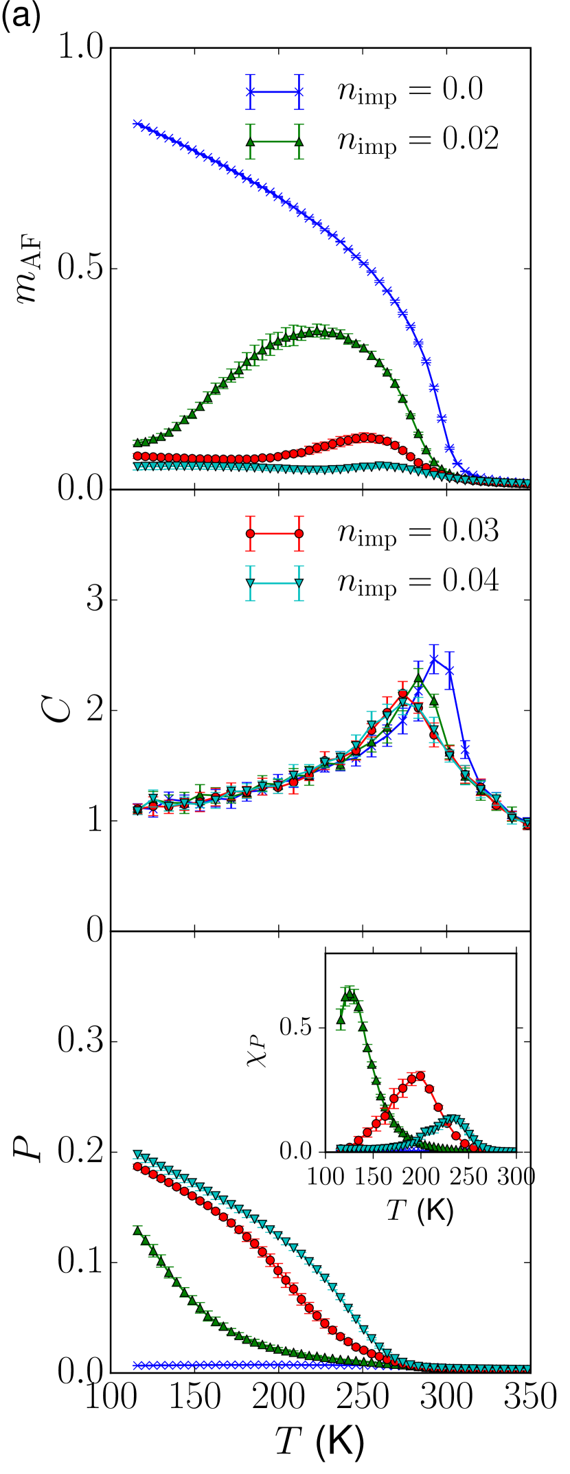
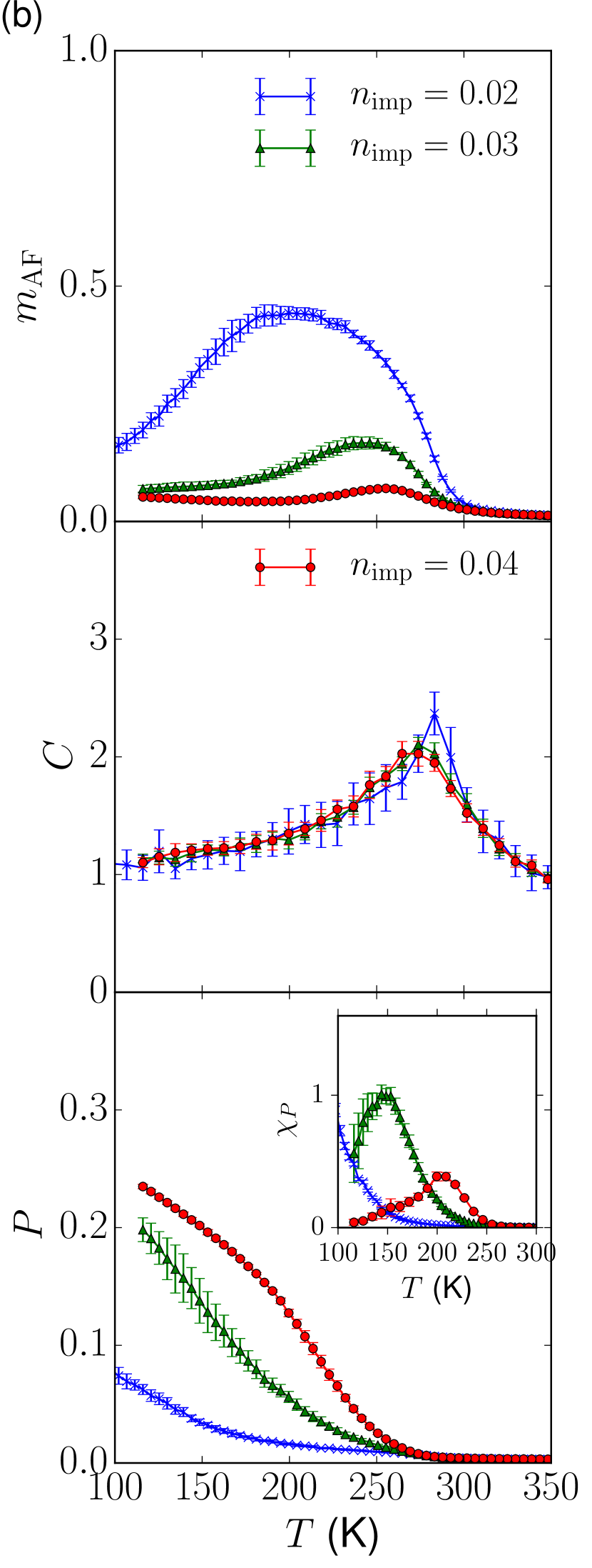
Figure S1: Results of MC simulations for the temperature dependence of the collinear order parameter $m_{\mathrm{AF}}$, the specific heat $C$, the polarization $P$, and electric susceptibility $\chi^{\,}_{\mathrm{P}}$ (inset of lowest panels) for $\xi_{\mathrm{min}}=4$ (a) and $\xi_{\mathrm{min}}=2.5$ (b) in units of in-plane lattice constant.

We start by discussing the $\xi_{\mathrm{min}}$ dependence of the results. Figure S1(a) shows MC data obtained for $L=28$ at $n^{\,}_{\mathrm{imp}}=0$, 0.02, 0.03, 0.04 for $\xi_{\mathrm{min}}=4$. Figure S1(b) shows the results for the case $\xi_{\mathrm{min}}=2.5$. For both values of $\xi_{\mathrm{min}}$, the low-temperature values of the collinear order parameter $m_{\mathrm{AF}}$ (upper panel) are suppressed as $n^{\,}_{\mathrm{imp}}$ is increased. Moreover, for $n^{\,}_{\mathrm{imp}}\neq 0$, $m_{\mathrm{AF}}$ shows the re-entrant behavior described in the main text as the temperature is decreased. Interestingly, for the case of $\xi^{\,}_{\mathrm{min}}=2.5$ the collinear antiferromagnetic order parameter $m^{\,}_{\mathrm{AF}}$ seems to not vanish completely at low temperatures for the lowest impurity concentration. This might either arise from finite size effects (too few windings of the spiral within the finite lattice) or indicate a possible coexistence of the magnetic spiral state with a collinear spin structure. The middle panels of Figs. S1(a) and S1(b) show the temperature dependence of the specific heat $C$. The peak position in $C$ coincides well with the onset of the collinear order parameter $m_{\mathrm{AF}}$ and is approximately unaffected by $n^{\,}_{\mathrm{imp}}$ and $\xi_{\mathrm{min}}$. The polarization $P$ (bottom panels) becomes nonvanishing below $T^{\,}_{\mathrm{spi}}$. For $T<T^{\,}_{\mathrm{spi}}$, $P$ increases continuously with decreasing $T$ to some saturation value at $T=0$. Hence, $T^{\,}_{\mathrm{spi}}$ is interpreted as the onset of the spiral phase through a continuous phase transition provided $n^{\,}_{\mathrm{imp}}>0$. The temperature below which the magnetic spiral state appears is better identifiable by the positions of the peaks of the dielectric susceptibility $\chi^{\,}_{P}$, defined as

$$\chi^{\,}_{P}:=\left\langle\frac{\left\langle\Pi^{2}\right\rangle^{\,}_{\mathrm{MC}}-\left\langle|\Pi|\right\rangle^{2}_{\mathrm{MC}}}{k^{\,}_{\mathrm{B}}TN}\right\rangle^{\,}_{\mathcal{L}}$$ (S7)

and shown in the insets of the lower panels in Fig. S1.

Figure S2 shows the dependence on $q^{\,}_{c}$ in Eq. (S5) of the spin-structure factor (S6) computed for eight different configurations of impurities. The size of the system and the minimal distance are set to $L=28$ and $\xi_{\mathrm{min}}=4$, respectively. One clearly sees a peak in the dependence of $S(q^{\,}_{c})$ on $q^{\,}_{c}$ at a value of $q^{\,}_{c}$ that deviates from $0.5$ as $n^{\,}_{\mathrm{imp}}$ is increased. This deviation approximately increases linearly with the concentration of impurity bonds $n^{\,}_{\mathrm{imp}}$, in agreement with the predictions of the low-temperature effective model.

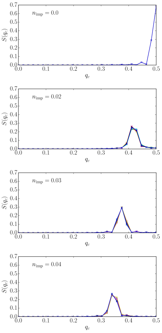
Figure S2: Spin structure factor $S(q^{\,}_{c})$ computed for different eight configurations of impurity bonds with $L=28$ and $\xi_{\mathrm{min}}=4$.

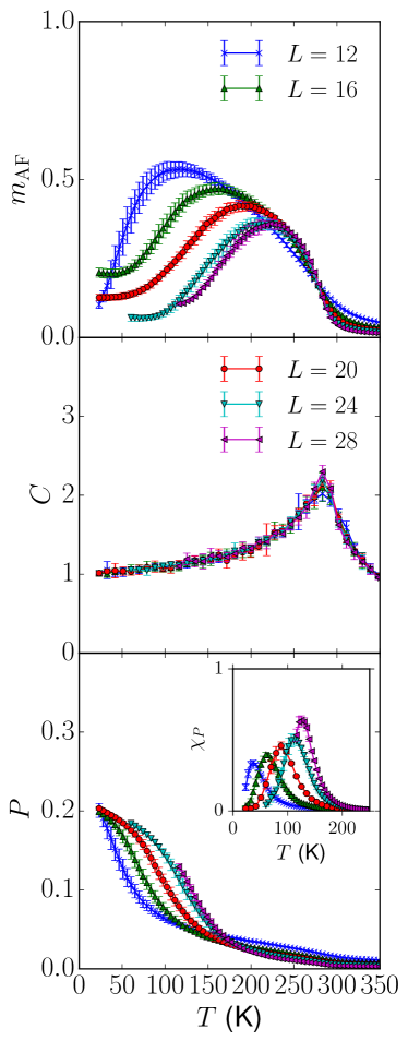
Figure S3: MC results for the temperature dependence of the collinear order parameter $m_{\mathrm{AF}}$, the specific heat $C$, the polarization $P$, and electric susceptibility $\chi^{\,}_{P}$ (inset) for various sizes of the lattice. The minimal distance is fixed at $\xi_{\mathrm{min}}=4$, while the concentration of impurity bonds is $n_{\mathrm{imp}}=0.02$.

To study the approach to the thermodynamic limit, we investigate the system-size dependence of the MC results for $n^{\,}_{\mathrm{imp}}=0.02$. As shown in Fig. S3, the dependence of $m_{\mathrm{AF}}$ on the system size is not monotonic around 120 K: $m_{\mathrm{AF}}$ has a small but non-vanishing residual value even at $L=28$. Therefore, as the system size is not large enough to obtain convergent results for $m_{\mathrm{AF}}$, we cannot exclude the possibility of the coexistence of the spin collinear order and the spin spiral order at low temperatures. On the other hand, $P$ converges with increasing $L$ rapidly for the lowest temperature considered to a nonvanishing and finite value. For example, at $T\simeq 23$ K, $P$ does not change appreciably when increasing $L$ from $L=12$ to $L=28$. This observation establishes the existence of the spin-spiral state at low $T$. However, the peak position in $\chi^{\,}_{P}$ drifts toward high temperatures as the system size is increased. This indicates that our calculations might actually underestimate the value of $T^{\,}_{\mathrm{spi}}$. Figure S4 shows the system-size dependence of $T_{\mathrm{N}}$ (peak position in $C$) and $T_{\mathrm{spi}}$ (peak position in $\chi^{\,}_{P}$). This clearly shows that $T_{\mathrm{spi}}$ is still monotonically increasing for $L$ increasing from 12 to 28, while $T^{\,}_{N}$ is approximately constant for $L$ increasing from 12 to 28.

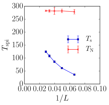
Figure S4: System-size dependence of the peak positions in the specific heat $C$ ($T_{\mathrm{N}}$) and the susceptibility $\chi^{\,}_{P}$ ($T_{\mathrm{spi}}$) at $n_{\mathrm{imp}}=0.02$ and $\xi_{\mathrm{min}}=4$.

Although our MC results for given large $L\times L\times L$ strongly suggest the existence of a finite $T_{\mathrm{spi}}$, extrapolating $T_{\mathrm{spi}}$ in the thermodynamic limit $L\to\infty$ with $n^{\,}_{\mathrm{imp}}$ held fixed is difficult. Furthermore, the transition may be sensitive to the geometry of the system since the effective interactions between impurity bonds are long ranged. Thus, we systematically study the geometry dependence of the spin-spiral transition. Figure S5 compares $T_{\mathrm{spi}}$ obtained for different geometries for $n^{\,}_{\mathrm{imp}}$=0.02 and $\xi_{\mathrm{min}}$=4. We adopt tetragonal shapes by which the dimensions $L\times L\times L$ are substituded by the dimensions $L^{\,}_{a}\times L^{\,}_{b}\times L^{\,}_{c}$ and we vary the ratio $L^{\,}_{a}/L^{\,}_{c}=L^{\,}_{b}/L^{\,}_{c}$ from 1 to 8. As the ratio $L^{\,}_{a}/L^{\,}_{c}$ becomes larger, $T_{\mathrm{spi}}$ tends to increase for the same numbers of spins $N^{\,}$. This trend is consistent with the dipole effective interaction, which is ferromagnetic in transverse directions $\boldsymbol{a}^{\prime}$ and $\boldsymbol{b}^{\prime}$. All the series of $T_{\mathrm{spi}}$ for different values of the $L^{\,}_{a}/L^{\,}_{c}$ ratio extrapolate to $T_{\mathrm{spi}}\simeq 200$ - $250$ K in the thermodynamic limit.

To confirm this result, we present the MC simulation for the Binder cumulant $g^{\,}_{P}$ of the the polarization $P$,

$$g^{\,}_{P}:=\left\langle\frac{1}{2}\left(3-\frac{\langle\Pi^{4}\rangle^{\,}_{\mathrm{MC}}}{\langle\Pi^{2}\rangle^{2}_{\mathrm{MC}}}\right)\right\rangle^{\,}_{\mathcal{L}},$$ (S8)

where $\Pi$ is defined by Eq. (S4b). The Binder cumulant is first computed for each configuration and then averaged over different configurations of impurity bonds. We show the temperature dependence of $g^{\,}_{P}$ for various values of the ratio $L^{\,}_{a}/L^{\,}_{c}$ in Fig. S6. One clearly sees an intersection of the data at $T_{\mathrm{spi}}\simeq 225$ K, which is lower than $T_{\mathrm{c}}$. The intersection of the Binder cumulants locates the value of $T^{\,}_{\mathrm{spi}}$ at $T_{\mathrm{spi}}\simeq 225$ K $<$ $T^{\,}_{\mathrm{N}}\simeq 275$ K.

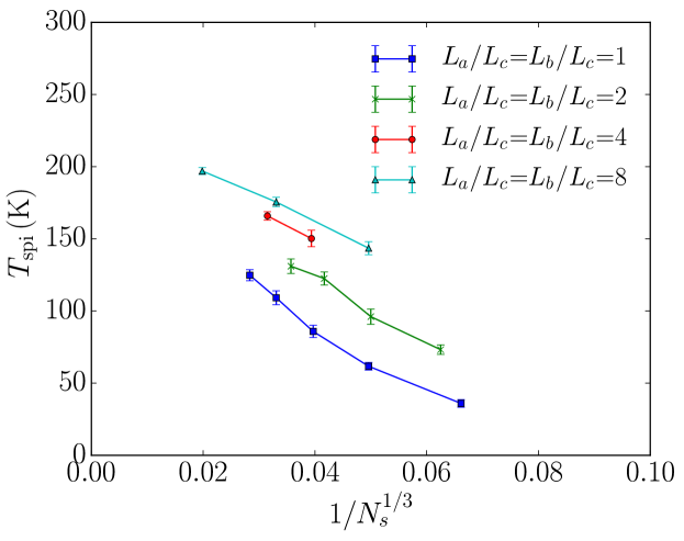
Figure S5: System-size dependence of the peak position in $\chi^{\,}_{P}$ for different geometries. The MC data were obtained for $n_{\mathrm{imp}}$=0.02 and $\xi_{\mathrm{min}}$=4.

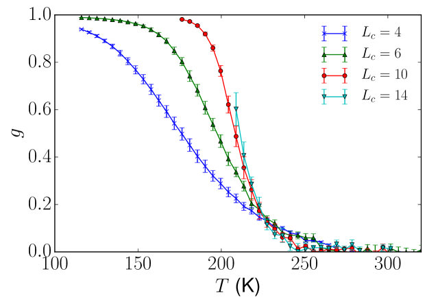
Figure S6: Binder cumulant of the polarization $P$ computed for $n_{\mathrm{imp}}$=0.02 and $\xi_{\mathrm{min}}$=4 with system sizes of $(8L^{\,}_{c},8L^{\,}_{c},L^{\,}_{c})$.

References

- Katsura et al. (2005) H. Katsura, N. Nagaosa, and A. V. Balatsky, Phys. Rev. Lett. 95, 057205 (2005).
- Mostovoy (2006) M. Mostovoy, Phys. Rev. Lett. 96, 067601 (2006).
- Khomskii (2009) D. Khomskii, Physics 2 (2009).
- Tokura and Seki (2010) Y. Tokura and S. Seki, Advanced Materials 22, 1554 (2010).
- Kimura (2007) T. Kimura, Annu. Rev. Mater. Res. 37, 387 (2007).
- Kimura et al. (2003) T. Kimura, T. Goto, H. Shintani, K. Ishizaka, T. Arima, and Y. Tokura, Nature 426, 55 (2003).
- Goto et al. (2004) T. Goto, T. Kimura, G. Lawes, A. P. Ramirez, and Y. Tokura, Physical Review Letters 92, 257201 (2004).
- Kenzelmann et al. (2005) M. Kenzelmann, A. B. Harris, S. Jonas, C. Broholm, J. Schefer, S. B. Kim, C. L. Zhang, S.-W. Cheong, O. P. Vajk, and J. W. Lynn, Phys. Rev. Lett. 95, 087206 (2005).
- Dong et al. (2008) S. Dong, R. Yu, S. Yunoki, J.-M. Liu, and E. Dagotto, Phys. Rev. B 78, 155121 (2008).
- Mochizuki and Furukawa (2009) M. Mochizuki and N. Furukawa, Phys. Rev. B 80, 134416 (2009).
- Kundys et al. (2009) B. Kundys, A. Maignan, and C. Simon, App. Phys. Lett. 94, 072506 (2009).
- Morin et al. (2015) M. Morin, A. Scaramucci, M. Bartkowiak, E. Pomjakushina, G. Deng, D. Sheptyakov, L. Keller, J. Rodriguez-Carvajal, N. A. Spaldin, M. Kenzelmann, K. Conder, and M. Medarde, Phys. Rev. B 91, 064408 (2015).
- Caignaert et al. (1995) V. Caignaert, I. Mirebeau, F. Bourée, N. Nguyen, A. Ducouret, J.-M. Greneche, and B. Raveau, J. Solid State Chem. 114, 24 (1995).
- Kawamura et al. (2010) Y. Kawamura, T. Kai, E. Satomi, Y. Yasui, Y. Kobayashi, M. Sato, and K. Kakurai, J. Phys. Soc. Jpn. 79, 073705 (2010).
- Ruiz-Aragón et al. (1998) M. J. Ruiz-Aragón, E. Morán, U. Amador, J. L. Martínez, N. H. Andersen, and H. Ehrenberg, Phys. Rev. B 58, 6291 (1998).
- (16) M. Morin, E. Canévet, A. Raynaud, M. Bartkowiak, D. Sheptyakov, B. Voraksmy, M. Kenzelmann, E. Pomjakushina, K. Conder, and M. Medarde, “Tuning magnetic spiral beyond room temperature with chemical disorder,” arXiv:1608.03372 [cond-mat.str-el] .
- Note (1) Note that the parameters used in this paper differ sligthly from those of Ref.\tmspace+.1667em \rev@citealpmorin_incommensurate_2015 as the LSDA+U method used to extract them in Ref.\tmspace+.1667em \rev@citealpmorin_incommensurate_2015 differs from the one used here.
- Ivanov et al. (1996) N. B. Ivanov, S. E. Krüger, and J. Richter, Phys. Rev. B 53, 2633 (1996).
- Capati et al. (2015) M. Capati, S. Caprara, C. Di Castro, M. Grilli, G. Seibold, and J. Lorenzana, Nature Communications 6, 7691 (2015).
- Edwards and Anderson (1975) S. F. Edwards and P. W. Anderson, J. Phys. F: Metal Physics 5, 965 (1975).
- Binder and Young (1986) K. Binder and A. P. Young, Rev. Mod. Phys. 58, 801 (1986).
- Villain (1977) J. Villain, J. Phys. C: Solid State Physics 10, 4793 (1977).
- Villain (1978) J. Villain, J. Phys. C: Solid State Physics 11, 745 (1978).
- Note (2) The antiferromagnetic Fe3+–Fe3+ coupling ranges between meV and meV in magnitude depending on the neighboring bipyramids. (We use the convention that the magnetic moments are of unit length.) Ab initio calculations were done using the same method as in Ref. Morin et al. (2015).
- Note (3) The magnetic exchange couplings have been rescaled so as to account for the magnitude of the classical magnetic moments of the ions located on the sites and .
- Note (4) Experiment shows that , which guarantees that the spiral has a cycloidal component. Note that a cycloidal component is a sufficient condition for the spiral order parameter to couple to the electric polarization. However, it is not a necessary condition when the impurity distribution breaks the two-fold rotation symmetry about an axis perpendicular to the spiral wave vector.
- (27) See on-line supplemental material.
- Scaramucci et al. (2016) A. Scaramucci, H. Shinaoka, M. V. Mostovoy, M. Müller, and C. Mudry, “Spiral order from orientationally correlated random bonds in classical xy models,” (2016), arXiv:1610.00784 .
- Note (5) We choose , , and such that the impurity bonds are confined to the bilayers of the host lattice as in YBaCuFeO5.
- Villain (1975) J. Villain, J. Phys. (Paris) 36, 581 (1975).
- Cox et al. (1963) D. E. Cox, W. J. Takei, and G. Shirane, J. Phys. Chem. Solids 24, 405 (1963).
- Utsumi et al. (2007) S. Utsumi, D. Yoshiba, and N. Momozawa, J. Phys. Soc. Jpn. 76, 034704 (2007).
- Momozawa et al. (1985) N. Momozawa, Y. Yamaguchi, H. Takei, and M. Mita, J. Phys. Soc. Jpn. 54, 771 (1985).
- Hukushima and Nemoto (1996) K. Hukushima and K. Nemoto, Journal of the Physical Society of Japan 65, 1604 (1996).
- Alonso et al. (1996) J. L. Alonso, A. Tarancón, H. G. Ballesteros, and L. A. Fernández, Physical Review B 53, 2537 (1996).
- Landau and Binder (2001) D. P. Landau and K. Binder, A Guide to Monte Carlo Simulations in Statistical Physics (2001).