Probing the diffractive production of gauge bosons at forward rapidities

Eduardo Basso¹, Victor P. Gonçalves², Murilo S. Rangel¹

¹ Instituto de Física, Universidade Federal do Rio de Janeiro, Caixa Postal 68528, Rio de Janeiro, RJ 21941-972, Brazil.

² Instituto de Física e Matemática, Universidade Federal de Pelotas, CEP 96010-900, Pelotas, RS, Brazil.

The gauge boson production at forward rapidities in single diffractive events at the LHC is investigated considering $pp$ collisions at $\sqrt{s}=$ 8 and 13 TeV. The impact of gap survival effects is analysed using two different models for the soft rescattering contributions. We demonstrate that using the Forward Shower Counter Project at LHCb – HERSCHEL, together with the Vertex Locator – VELO, it is possible to discriminate diffractive production of the gauge bosons $W$ and $Z$ from the non-diffractive processes and studies of the Pomeron structure and diffraction phenomenology are feasible. Moreover, we show that the analysis of this process can be useful to constrain the modelling of the gap survival effects.

1 Introduction

At present days one can say that Quantum Chromodynamics factorization [1, 2] has been thoroughly tested so that it can be taken as the most powerful tool describing high energy hadronic collisions. Usually, the hard perturbation contributions are well separated from the soft non-perturbative ones, which are encoded in the parton distributions functions (PDF). This idea was extended long ago to the case of diffractive deep inelastic scattering (DDIS), for which factorization proofs have been carefully proved (see [3] and references therein). Yet the Regge factorization of the diffractive dissociation into a two step process, as suggested long ago by Ingelman and Schlein (IS) [4] and not proven in pQCD, have been largely used to describe hard diffractive events in $ep$ collisions [5]. The IS approach essentially considers that the diffractive processes can be described in terms of the probability of the proton to emit a colour single object – the Pomeron – and the subsequent interaction of the partons inside such Pomeron with the virtual photon emitted by the incident electron. This introduces the Pomeron parton distribution functions, which can be extracted from data where a hard final state is produced and a leading hadron is detected.

When it comes to diffractive events in $pp$ collisions, however, one have to be careful using these ideas, since factorization has shown to be broken when going from DDIS at HERA to hadron-hadron collisions at the Tevatron and the LHC. Indeed, theoretical studies [6, 3] performed before the experimental confirmation predicted that the breakdown of the factorization due to soft rescattering corrections associated to reinteractions (often referred to as multiple scatterings) between spectator partons of the colliding hadrons. These processes can produce additional final - state particles which fill the would-be rapidity gap and suppress the diffractive events. Consequently, in order to estimate the diffractive cross sections in hadronic collisions we need to take into account for the probability that such emission does not occur. One possible approach to treat this problem is to assume that the hard process occurs on a short enough timescale such that the physics that generate the additional particles can be factorized and accounted by an overall factor, denoted gap survival factor $\left<S^{2}\right>$, multiplying the cross section calculated using the collinear factorization and the diffractive parton distributions extracted from HERA data. The modelling and magnitude of this factor still is a theme of intense debate [7, 8, 9]. In general the values of $\left<S^{2}\right>$ depend on the energy, being typically of order $1-5$% for LHC energies [10, 11]. Such approach have been largely used in the literature to estimate the hard diffractive processes at the LHC (See e.g. Refs. [12, 13, 14, 15, 16, 17, 18, 19, 20, 21]) with reasonable success to describe the current data. On the other hand, a distinct approach to treat the soft rescattering interactions that destroy the rapidity gap have been proposed very recently [22]. The basic idea is to explore the fact that the diffractive factorization breaking effects are intimately related to multiple scattering in hadronic collisions. They start from the IS approach and adds a dynamically calculated rapidity gap survival factor, derived from the modelling of multiparton interactions as implemented in the Pythia 8  [23]. The dynamical gap survival (DGS) describes the factorization breaking as a function of the hard process studies and its kinematics. As demonstrated in Ref. [22], its predictions are in reasonable agreement with current data.

In order to constrain the modelling of the gap survival effects and improve our limited understanding of diffraction it is fundamental to experimentally discriminate the diffractive production from the non-diffractive processes. The experimental signature for e.g. single diffractive production is either the presence of one rapidity gap in the detector or a proton tagged in the final state. Forward proton detectors at ATLAS and CMS experiments are in general available in special data taking periods with low integrated luminosity [24]. There are plans to operate these in nominal data taking with very reduced acceptance for masses smaller than few hundred GeV. On the other hand, due to the lower instantaneous luminosity present at the LHCb experiment, it is possible to benefit from its low pile-up conditions and its ability to reject activity in the backward region, to perform the study of the single diffractive processes at the LHCb. Such advantages have been demonstrated in the study of the heavy quark production in photon and Pomeron induced interactions performed in Ref. [19].

The LHCb detector is a single-arm spectrometer covering the forward region of $2<\eta<5$ [25]. Recently, the LHCb collaboration published studies of the $W$ and $Z$ production inclusively  [26, 27, 28, 29] and in association with jets [30, 31, 32, 33]. These results show great ability of the LHCb experiment to make precise measurements of forward $W$ and $Z$ boson production. In addition, the LHCb experiment is also able to reject activity in the backward region using tracks reconstructed in the Vertex Locator (VELO) sub-detector. The experiment runs at lower instantaneous luminosity benefiting from low pile-up conditions. Indeed, LHCb has already published central exclusive analyses exploring the ability of requiring a backward gap [34, 35, 36] in RunI. New results of LHCb central exclusive production has also been available using the new forward shower counters [37] that extends the pseudorapidity region in which charged particles can be vetoed [38]. Additionally, at the Run II, it is possible to study diffractive events at the LHCb experiment by selecting the muon within the LHCb acceptance and require no particles in the backward region of $-3.5<\eta<-1.5$ (VELO) and $-8.0<\eta<-5.5$ (HERSCHEL).

In this paper we study the gauge boson production in single diffractive events and propose to use the HERSCHEL, together with the VELO, to discriminate diffractive production of the gauge bosons $W$ and $Z$ from the non-diffractive processes. The results presented here indicate that studies of the Pomeron structure and diffraction phenomenology are feasible at the LHC and that the analysis of this process can be useful to constrain the modelling of the gap survival effects. The paper is organized as follows. In the next Section we present a brief review of the formalism used for the gauge boson production in single diffractive events. In Section 3 we present our results for the total cross sections and pseudorapidity distributions. We consider the $W$ and $Z$ production as well as its production associated to a jet and estimate the ratio between cross sections, which cancel several of the experimental and theoretical systematic uncertainties, considering $pp$ collisions at $\sqrt{s}=$ 8 and 13 TeV and two distinct models for the gap survival effects. Finally, in Section 4 we summarize our main conclusions.

2 Single diffractive gauge boson production

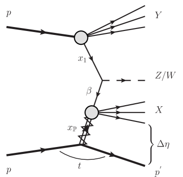
Figure 1: LO diagram contributing to single diffractive production of gauge bosons.

In the following we apply the IS approach [4] for the diffractive gauge boson production represented in Fig. 1. This model, denoted often Resolved Pomeron Model, assumes that the Pomeron has a well defined partonic structure and that the hard process takes place in a Pomeron - proton or proton - Pomeron interaction in the case of single diffractive processes. At leading order the gauge boson production is determined by the annihilation processes $q\bar{q}\rightarrow G$ ($G=W$ or $Z$). Higher order contributions are not considered here and can be taken into account effectively by a $K$ factor. In order to estimate the hadronic cross sections we have to convolute the cross section for this partonic subprocess with the inclusive and diffractive parton distribution functions. In the collinear factorization formalism, the single diffractive gauge boson production cross section can be expressed by

$$\sigma^{SD}(pp\rightarrow Gp)=\sum_{a,b}\int dx_{a}\int dx_{b}\left[f^{D}_{a}(x_{a},\mu^{2})f_{b}(x_{b},\mu^{2})+f_{a}(x_{a},\mu^{2})f^{D}_{b}(x_{b},\mu^{2})\right]\,\hat{\sigma}_{ab\rightarrow G}\,\,,$$ (1)

where $f_{i}(x_{i},\mu^{2})$ and $f_{i}^{D}(x_{i},\mu^{2})$ are the inclusive and diffractive parton distribution functions, respectively, and we included both $p\mathbb{P}$ and $\mathbb{P}p$ interactions. Moreover, $\hat{\sigma}_{ab\rightarrow G}$ denotes the hard partonic interaction producing a gauge boson.

The Resolved Pomeron Model considers the difractive parton distributions as a convolution of the Pomeron flux emitted by the proton, $f_{\mathbb{P}}(x_{\mathbb{P}})$, and the parton distributions in the Pomeron, $g_{\mathbb{P}}(\beta,\mu^{2})$, $q_{\mathbb{P}}(\beta,\mu^{2})$, where $\beta$ is the momentum fraction carried by the partons inside the Pomeron. The Pomeron flux is given by $f_{\mathbb{P}}(x_{\mathbb{P}})=\int_{t_{min}}^{t_{max}}dtf_{\mathbb{P}/p}(x_{{\mathbb{P}}},t)$, where

$$f_{\mathbb{P}/p}(x_{\mathbb{P}},t)=A_{\mathbb{P}}\frac{e^{B_{\mathbb{P}}t}}{x_{\mathbb{P}}^{2\alpha_{\mathbb{P}}(t)-1}}\,.$$ (2)

The normalization of the flux is such that the relation $x_{\mathbb{P}}\int^{t_{\text{min}}}_{{t_{\text{cut}}}}{\mathrm{d}}tf_{\mathbb{P}/p}(x_{\mathbb{P}},t)=1$ holds at $x_{\mathbb{P}}=0.003$, where $|t_{\text{cut}}|=1$ GeV is limited by the measurement and $|t_{\text{min}}|\simeq(m_{\text{p}}x_{\mathbb{P}})^{2}/(1-x_{\mathbb{P}})$ is the kinematic limit of accessible momentum $|t|$. The Pomeron flux factor is motivated by Regge theory, where the Pomeron trajectory assumed to be linear, $\alpha_{\mathbb{P}}(t)=\alpha_{\mathbb{P}}(0)+\alpha_{\mathbb{P}}^{\prime}t$, and the parameters $B_{\mathbb{P}}$, $\alpha_{\mathbb{P}}^{\prime}$ and their uncertainties are obtained from fits to H1 data [39, 40]. The diffractive quark and gluon distributions are then given by

$${q^{D}(x,\mu^{2})}=\int dx_{\mathbb{P}}d\beta\delta(x-x_{\mathbb{P}}\beta)f_{\mathbb{P}}(x_{\mathbb{P}})q_{\mathbb{P}}(\beta,\mu^{2})={\int_{x}^{1}\frac{dx_{\mathbb{P}}}{x_{\mathbb{P}}}f_{\mathbb{P}}(x_{\mathbb{P}})q_{\mathbb{P}}\left(\frac{x}{x_{\mathbb{P}}},\mu^{2}\right)}\,,$$ (3)

$${g^{D}(x,\mu^{2})}=\int dx_{\mathbb{P}}d\beta\delta(x-x_{\mathbb{P}}\beta)f_{\mathbb{P}}(x_{\mathbb{P}})g_{\mathbb{P}}(\beta,\mu^{2})={\int_{x}^{1}\frac{dx_{\mathbb{P}}}{x_{\mathbb{P}}}f_{\mathbb{P}}(x_{\mathbb{P}})g_{\mathbb{P}}\left(\frac{x}{x_{\mathbb{P}}},\mu^{2}\right)}\,.$$ (4)

In the present analysis the H1 Fit A is used [39, 40], which has the slope parameter set to $B_{\mathbb{P}}=5.5$ GeV^-2 and $\alpha_{\mathbb{P}}^{\prime}=0.06$ GeV^-2, while $\alpha_{\mathbb{P}}(0)=1.118\pm 0.008$. Moreover, we use the inclusive parton distributions as given by the CT10 parametrization [41]. It is important to emphasize that at large values of the Pomeron longitudinal $x_{\mathbb{P}}$, subleading contributions associated to Reggeon exchange can be important in some regions of the phase space (For a recent discussion see e.g. Ref. [20]). In what follows we disregard this contribution and postpone for a future study the analysis of its impact.

Recently, the Resolved Pomeron Model described above have been implemented in Pythia 8 [22], allowing to estimate the hard diffractive events at the LHC using this event generator. However, in order to describe the data for diffractive events in $pp$ collisions we should taken into account the soft rescattering contributions discussed in the Introduction and that imply the breakdown of the diffractive factorization. In the last years, many models have been proposed to describe the Gap Survival Probability (GSP). A simplistic approach is based on the assumption that the soft rescattering contributions can be factorized from the hard processes and can be taken into account as a multiplicative factor to the cross section. Such models were shortly summarized recently in [8], with its value being typically of order $1-5$% for LHC energies, according to the calculations of the Durham (2 channel eikonal model) [10] and Tel-Aviv [11] groups. On the other hand, there are a few approaches aiming to model the GSP as a dynamical process [42, 43, 44, 45, 46, 47]. In particular, in Ref. [22] the authors have proposed to use the full machinery of Multiple Parton Interactions (MPI) present in the Pythia 8 generator to account for the absorptive corrections upon which the GSP are built. The basic idea is that the MPI that occur between the incoming hadrons can create colour flows that fill with hadrons the rapidity range available, destroying the rapidity gap associated to single diffractive events. Since MPI are dynamically generated, the GSP obtained from such method is also dynamical. When this framework is switched off, “pure” diffractive events are generated and the factorization breaking events should be additionally included through a multiplicative factor. In what follows we will consider both prescriptions to treat the GSP, denoting by SD1 those derived assuming that $\left<S^{2}\right>=0.05$ at the LHC energies, as in Refs. [12, 13, 14, 15, 16, 17, 18, 19, 20, 21], and by SD2 those associated the dynamically generated gap survival based on MPI as implemented in Pythia 8 [22]. The comparison between these two models for the GSP allows to estimate the current theoretical uncertainty in the predictions for diffractive events in comparison to the non-diffractive (ND) events, which will be studied here as well.

3 Results

In what follows we present results for the $W$ and $Z$ production in $pp$ collisions at $\sqrt{s}=8$ and $13\mathrm{\,Te\kern-1.00006ptV}$. The main focus will be in forward region covered by the LHCb detector. The events have been generated in Pythia 8 and we have selected the muon within the LHCb acceptance and required no particles in the backward region of $-3.5<\eta<-1.5$ (VELO) and $-8.0<\eta<-5.5$ (HERSCHEL). The VELO gap requirement is performed using charged particles with momentum greater than $100\mathrm{\,Me\kern-1.00006ptV}$. We assumed that the HERSCHEL is able to detect charged and neutral with $\mbox{$p_{\rm T}$}>0.5\mathrm{\,Ge\kern-1.00006ptV}$. Additionally, the gauge boson selection used in Ref. [33] have been applied, i.e., the $W$ boson is identified using its decay to a muon and a neutrino and the Z boson is identified using its decay to a muon pair. The muon must have $\mbox{$p_{\rm T}$}(\mu)>20\mathrm{\,Ge\kern-1.00006ptV}$ and $2.0<\eta(\mu)<4.5$.

	$\sqrt{s}=13\mathrm{\,Te\kern-1.00006ptV}$		$\sqrt{s}=8\mathrm{\,Te\kern-1.00006ptV}$
Process	No gap	VH gap	No gap	V gap
$W^{+}$ ND	$1.7\times 10^{3}$	$4.4$	$1.4\times 10^{3}$	$15$
$W^{+}$ SD1	$15$	$1.7$	$12$	$1.6$
$W^{+}$ SD2	$48$	$5.6$	$41$	$5.1$
$W^{-}$ ND	$1.2\times 10^{3}$	$3.6$	$1.1\times 10^{3}$	$12$
$W^{-}$ SD1	$10$	$0.9$	$9.4$	$0.94$
$W^{-}$ SD2	$35$	$3.0$	$32$	$3.1$
$Z$ ND	$150$	$0.38$	$100$	$1.3$
$Z$ SD1	$1.4$	$0.15$	$0.9$	$0.12$
$Z$ SD2	$4.4$	$0.50$	$3.0$	$0.42$

Table 1: Cross-sections in $\rm\,pb$ for $W$ and $Z$ production in the LHCb fiducial region before and after requiring a region void of particles for 8 and 13 TeV. For 13 TeV the gap requirement considers the VELO and HERSCHEL detectors (VH gap) while for 8 TeV only VELO detector is used (V gap).

Predictions for the cross-sections in the LHCb fiducial region are presented in Table 1 for $pp$ collisions at 8 and $13\mathrm{\,Te\kern-1.00006ptV}$. We present the results obtained before and after requiring a region void of particles (gap) in the final state. For 13 TeV the gap requirement considers the VELO and HERSCHEL detectors (denoted VH gap) while for 8 TeV only VELO detector is used (denoted V gap). As expected, we have that if the gap requirement is not assumed, the non-diffractive (ND) production of gauge bosons is dominant, being two orders of magnitudes larger than the single diffraction (SD) one. On the other hand, if a gap is required, the ND contribution is strongly suppressed and becomes of the order of the SD process. In particular, such suppression is larger at $\sqrt{s}=13$ TeV, which demonstrates the impact of the HERSCHEL detector for the study of diffractive events. Regarding the models for the gap survival, we have that its predictions are similar, with the SD1 model predicting cross sections that are a factor 3 smaller than the SD2 one. An important aspect is that the SD2 model implies that the single diffraction production of $W^{+}$ and $Z$ becomes dominant at 13 TeV. This results motivates the analysis of differential distributions that can be measured experimentally. In Fig. 2 we present the predictions for the differential cross-section as function of the pseudorapidity of the muon $\eta(\mu)$ for the $W^{+}$ production. In the left (right) panel we show the results obtained before (after) the gap requirement is applied. One can see that the additional HERSCHEL gap requirement improves the discrimination between non-diffractive and diffrative processes for $13\mathrm{\,Te\kern-1.00006ptV}$ prediction and implies that SD contribution becomes dominant in a large range of pseudorapidities in the case of the SD2 model.

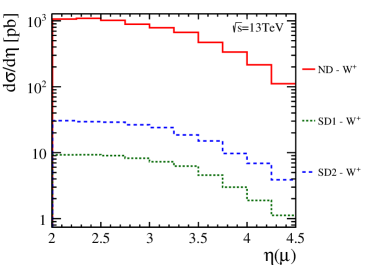
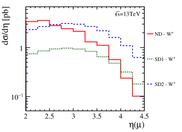
Figure 2: Differential cross-section as function of $\eta(\mu)$ for non-diffractive and single-diffrative production of $W$ in $pp$ collisions at $\sqrt{s}=$ 13 TeV before (left) and after (right) the gap requirement is assumed.

In order to minimize possible experimental and theoretical systematic uncertainties we propose the analysis of the ratios between the cross sections defined by ${R_{{W^{\pm}}}}=\frac{\sigma_{W^{+}}}{\sigma_{W^{-}}}$, ${R_{{W^{-}}Z}}=\frac{\sigma_{W^{-}}}{\sigma_{Z}}$ and ${R_{{W^{+}}Z}}=\frac{\sigma_{W^{+}}}{\sigma_{Z}}$. The error in the ratios $R_{{W^{-}}Z}$ and $R_{{W^{+}}Z}$ is dominated by sample size. As we are interested in investigate the impact of the single diffraction contribution we will estimate these ratio considering only the ND contribution and will compare these with those obtained summing the ND and SD contributions. Assuming an integrated luminosity of $\int\mathcal{L}=5$ $\mbox{\,fb}^{-1}$ for 13 TeV and $\int\mathcal{L}=2$ $\mbox{\,fb}^{-1}$ for 8 TeV, we have estimated these ratios and the predictions with their respective expected statistical errors are shown in Fig. 3. One have that for $\sqrt{s}=$ 8 TeV the impact of the SD contribution is smaller than 10 %. On the other hand, for $\sqrt{s}=$ 13 TeV and for the ratios ${R_{{W^{\pm}}}}=\frac{\sigma_{W^{+}}}{\sigma_{W^{-}}}$ and ${R_{{W^{+}}Z}}=\frac{\sigma_{W^{+}}}{\sigma_{Z}}$, one have that its contribution can be of the order of 20 % and is sensitive to the model used for the description of the gap survival effects.

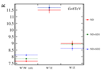
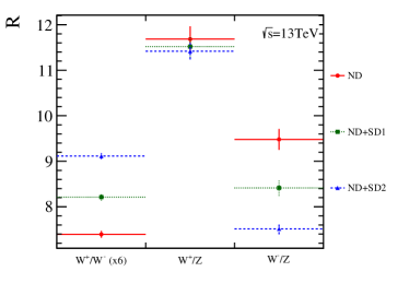
Figure 3: Ratio of cross-sections for $W$ and $Z$ production: ${R_{{W^{\pm}}}}=\frac{\sigma_{W^{+}}}{\sigma_{W^{-}}}$, ${R_{{W^{-}}Z}}=\frac{\sigma_{W^{-}}}{\sigma_{Z}}$ and ${R_{{W^{+}}Z}}=\frac{\sigma_{W^{+}}}{\sigma_{Z}}$. The displayed errors are the expected statistical errors considering $\int\mathcal{L}=5$ $\mbox{\,fb}^{-1}$ for 13 TeV and $\int\mathcal{L}=2$ $\mbox{\,fb}^{-1}$ for 8 TeV. ${R_{{W^{\pm}}}}$ is multiplied by 6.

	$\sqrt{s}=13\mathrm{\,Te\kern-1.00006ptV}$		$\sqrt{s}=8\mathrm{\,Te\kern-1.00006ptV}$
Process	No gap	VH gap	No gap	V gap
$W^{+}$ $j$ ND	$3.3\times 10^{2}$	$0.37$	$2.1\times 10^{2}$	$1.2$
$W^{+}$ $j$ SD1	$2.5$	$0.2$	$1.6$	$0.15$
$W^{+}$ $j$ SD2	$8.2$	$0.65$	$5.5$	$0.49$
$W^{-}$ $j$ ND	$2.3\times 10^{2}$	$0.29$	$1.5\times 10^{2}$	$1.0$
$W^{-}$ $j$ SD1	$1.6$	$0.1$	$1.1$	$0.08$
$W^{-}$ $j$ SD2	$5.4$	$0.35$	$3.7$	$0.29$
$Z$ $j$ ND	$31$	$0.03$	$17$	$0.12$
$Z$ $j$ SD1	$0.25$	$0.02$	$0.14$	$0.01$
$Z$ $j$ SD2	$0.86$	$0.07$	$0.45$	$0.05$

Table 2: Cross-sections in $\rm\,pb$ for $W$/$Z$ plus jets production before and after requiring a region void of particles for $\sqrt{s}=$ 8 and 13 TeV. For 13 TeV the gap requirement considers the VELO and HERSCHEL detectors (VH gap) while for 8 TeV only VELO detector is used (V gap).

In addition to the study of the inclusive gauge boson production, which is strongly dependent on the quark distribution of the proton and of the Pomeron, the associate production with jets can be useful since it also is sensitive to the gluon distribution. In order to evaluate the impact of single diffractive contribution in gauge boson plus jets at LHCb, we have reconstructed the jet using the $\text{anti-}k_{\mathrm{T}}$ algorithm [48] with distance parameter $R=0.5$ as implemented in the FastJet software package [49]. In the $W$/$Z$ plus jet selection, jets were required to have $\mbox{$p_{\rm T}$}(\text{jet})>10\mathrm{\,Ge\kern-1.00006ptV}$, $2.2<\eta(\text{jet})<4.2$ and $\Delta\text{\it R}({\mu},\text{jet})>0.5$, where $\Delta\text{\it R}=\sqrt{\Delta\varphi^{2}+\Delta\eta^{2}}$. The results for the cross-sections in the LHCb fiducial region are presented in Table 2 for 8 and $13\mathrm{\,Te\kern-1.00006ptV}$ with and without gap requirements. As in the inclusive gauge boson production, the ND contribution is dominant in the gauge boson + jet production if a gap is not required in the final state and highly suppressed if the gap is required. Moreover, the SD2 model predicts the dominance of the single diffraction production at $\sqrt{s}=13$ TeV if the gap requirement considers the VELO and HERSCHEL detectors. This behaviour is also present in the differential distributions. As a example, in Fig.  4 we present predictions for the $W^{+}$ plus jet production in $pp$ collisions at $\sqrt{s}=13$ TeV before (left panel) and after (right panel) the implementation of the gap requirement. One have that in the case of the SD2 model, the single diffractive $W^{+}$ plus jet production is dominant for all values of pseudorapidity covered by the LHCb detector.

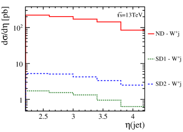
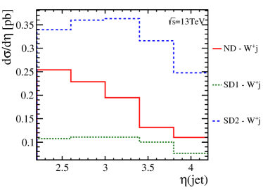
Figure 4: Differential cross-section as function $\eta({\rm jet})$ for non-diffractive and single-diffrative production of $W^{+}$ plus jets in $pp$ collisions at $\sqrt{s}$ = 13 TeV before (left) and after (right) the implementation of the gap requirement.

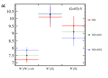
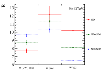
Figure 5: Ratio of cross-sections for $W$ and $Z$ production in association with jets: $R_{1}=\frac{\sigma_{{W^{+}}j}}{\sigma_{{W^{-}}j}}$, $R_{2}=\frac{\sigma_{{W^{-}}j}}{\sigma_{Zj}}$ and $R_{3}=\frac{\sigma_{{W^{+}}j}}{\sigma_{Zj}}$. The displayed errors are the expected statistical errors considering $\int\mathcal{L}=5$ $\mbox{\,fb}^{-1}$ for 13 TeV and $\int\mathcal{L}=2$ $\mbox{\,fb}^{-1}$ for 8 TeV. $R_{1}$ is multiplied by 6.

Finally, in Fig. 5 we present the predictions for $R_{1}=\frac{\sigma_{{W^{+}}j}}{\sigma_{{W^{-}}j}}$, $R_{2}=\frac{\sigma_{{W^{-}}j}}{\sigma_{Zj}}$ and $R_{3}=\frac{\sigma_{{W^{+}}j}}{\sigma_{Zj}}$. As in the inclusive production, one have that these ratios are sensitive to the presence of the single diffractive events and its magnitude depends of the model used to describe the gap survival effects.

4 Summary

In this paper we investigated the gauge boson production at forward rapidities in single diffractive events at the LHC. Using the Pythia 8 event generator we have estimated the cross sections and differential distributions for the $W^{+}$, $W^{-}$ and $Z$ production, as well for the gauge boson production in association with jets. We have considered realistic cuts and gap requirements that can be performed by the LHCb Collaboration. The present analysis is complementary to the studies involving the planned proton tagging detectors by CMS and ATLAS collaborations, with the advantage that LHCb is already setup for detection of diffractive events. Our results demonstrated that using the HERSCHEL, in addition to the VELO, it is possible to discriminate diffractive production of the gauge bosons $W$ and $Z$ (with and without extra jets) from the non-diffractive processes. As a consequence, it is possible to use the resulting experimental data to study in more detail the treatment of the diffractive processes. In particular, our results shown that the analysis of the cross sections, differential distributions and the ratio between cross sections can be useful to constrain the model used for the soft rescattering corrections that breakdown the diffractive factorization in hadronic collisions.

References

- [1] J. C. Collins, D. E. Soper, and G. F. Sterman, Factorization for Short Distance Hadron - Hadron Scattering, Nucl. Phys. B261 (1985) 104
- [2] J. C. Collins, D. E. Soper, and G. F. Sterman, Soft Gluons and Factorization, Nucl. Phys. B308 (1988) 833
- [3] J. C. Collins, Proof of factorization for diffractive hard scattering, Phys. Rev. D57 (1998) 3051, arXiv:hep-ph/9709499, [Erratum: Phys. Rev.D61,019902(2000)]
- [4] G. Ingelman and P. E. Schlein, Jet Structure in High Mass Diffractive Scattering, Phys. Lett. B152 (1985) 256
- [5] ZEUS, H1 Collaboration, F. D. Aaron et al., Combined inclusive diffractive cross sections measured with forward proton spectrometers in deep inelastic scattering at HERA, Eur. Phys. J. C72 (2012) 2175, arXiv:1207.4864
- [6] J. D. Bjorken, Rapidity gaps and jets as a new-physics signature in very-high-energy hadron-hadron collisions, Phys. Rev. D 47 (1993) 101
- [7] V. A. Khoze, A. D. Martin, and M. G. Ryskin, Elastic scattering and Diffractive dissociation in the light of LHC data, Int. J. Mod. Phys. A30 (2015), no. 08 1542004, arXiv:1402.2778
- [8] E. Gotsman, E. Levin, and U. Maor, A comprehensive model of soft interactions in the LHC era, Int. J. Mod. Phys. A30 (2015), no. 08 1542005, arXiv:1403.4531
- [9] B. Kopeliovich, R. Pasechnik, and I. Potashnikova, Hard hadronic diffraction is not hard, Int. J. Mod. Phys. E25 (2016), no. 07 1642001, arXiv:1603.08468
- [10] V. A. Khoze, A. D. Martin, and M. G. Ryskin, Diffraction at the LHC, Eur. Phys. J. C73 (2013) 2503, arXiv:1306.2149
- [11] E. Gotsman, E. Levin, and U. Maor, Survival probability of large rapidity gaps in QCD and N=4 SYM motivated model, Eur. Phys. J. C71 (2011) 1685, arXiv:1101.5816
- [12] M. B. Gay Ducati, M. M. Machado, and M. V. T. Machado, Diffractive hadroproduction of and bosons at high energies, Phys. Rev. D75 (2007) 114013, arXiv:hep-ph/0703315
- [13] M. Luszczak, R. Maciula, and A. Szczurek, Single- and central-diffractive production of open charm and bottom mesons at the LHC: theoretical predictions and experimental capabilities, Phys. Rev. D91 (2015), no. 5 054024, arXiv:1412.3132
- [14] C. Brenner Mariotto and V. P. Goncalves, Diffractive photon production at the LHC, Phys. Rev. D88 (2013), no. 7 074023, arXiv:1309.2026
- [15] C. Marquet, C. Royon, M. Saimpert, and D. Werder, Probing the Pomeron structure using dijets and +jet events at the LHC, Phys. Rev. D88 (2013), no. 7 074029, arXiv:1306.4901
- [16] A. Chuinard, C. Royon, and R. Staszewski, Testing Pomeron flavour symmetry with diffractive W charge asymmetry, JHEP 04 (2016) 092, arXiv:1510.04218
- [17] M. Luszczak, A. Szczurek, and C. Royon, pair production in proton-proton collisions: small missing terms, JHEP 02 (2015) 098, arXiv:1409.1803
- [18] C. Brenner Mariotto and V. P. Goncalves, Double production in central diffractive processes at the LHC, Phys. Rev. D91 (2015), no. 11 114002, arXiv:1502.02612
- [19] V. P. Goncalves, C. Potterat, and M. S. Rangel, Bottom production in Photon and Pomeron – induced interactions at the LHC, Phys. Rev. D93 (2016), no. 3 034038, arXiv:1511.07688
- [20] C. Marquet et al., Diffractive di-jet production at the LHC with a Reggeon contribution, arXiv:1608.05674
- [21] M. Luszczak, R. Maciula, A. Szczurek, and M. Trzebinski, Single-diffractive production of charmed mesons at the LHC within the -factorization approach, arXiv:1606.06528
- [22] C. O. Rasmussen and T. Sjöstrand, Hard Diffraction with Dynamic Gap Survival, JHEP 02 (2016) 142, arXiv:1512.05525
- [23] T. Sjöstrand et al., An Introduction to PYTHIA 8.2, Comput. Phys. Commun. 191 (2015) 159, arXiv:1410.3012
- [24] LHC Forward Physics Working Group, e. Royon, C. et al., LHC Forward Physics, CERN-PH-LPCC-2015-001, SLAC-PUB-16364, DESY-15-167 (2015)
- [25] LHCb Collaboration, R. Aaij et al., LHCb detector performance, Int. J. Mod. Phys. A30 (2015) 1530022, arXiv:1412.6352
- [26] LHCb Collaboration, R. Aaij et al., Measurement of the forward boson production cross-section in collisions at TeV, LHCb-PAPER-2016-021, in preparation
- [27] LHCb Collaboration, R. Aaij et al., Measurement of the forward boson production cross-section in collisions at TeV, JHEP 12 (2014) 079, arXiv:1408.4354
- [28] LHCb Collaboration, R. Aaij et al., Measurement of the forward boson cross-section in collisions at TeV, JHEP 08 (2015) 039, arXiv:1505.07024
- [29] LHCb Collaboration, R. Aaij et al., Measurement of forward and boson production in collisions at TeV , JHEP 01 (2015) 155, arXiv:1511.08039
- [30] LHCb Collaboration, R. Aaij et al., Study of forward +jet production in collisions at TeV, JHEP 01 (2014) 033, arXiv:1310.8197
- [31] LHCb Collaboration, R. Aaij et al., Measurement of the +-jet cross-section in collisions at TeV in the forward region, JHEP 01 (2015) 064, arXiv:1411.1264
- [32] LHCb Collaboration, R. Aaij et al., Study of boson production in association with beauty and charm, Phys. Rev. D92 (2015) 052012, arXiv:1505.04051
- [33] LHCb Collaboration, R. Aaij et al., Measurement of forward and boson production in association with jets in proton-proton collisions at TeV, JHEP 05 (2016) 131, arXiv:1605.00951
- [34] LHCb Collaboration, R. Aaij et al., Measurement of the exclusive Υ production cross-section in pp collisions at TeV and 8 TeV, JHEP 09 (2015) 084, arXiv:1505.08139
- [35] LHCb Collaboration, R. Aaij et al., Updated measurements of exclusive and (2S) production cross-sections in pp collisions at TeV, J. Phys. G41 (2014) 055002, arXiv:1401.3288
- [36] LHCb Collaboration, R. Aaij et al., Observation of charmonium pairs produced exclusively in collisions, J. Phys. G41 (2014), no. 11 115002, arXiv:1407.5973
- [37] K. C. Akiba et al., The Herschel detector: high rapidity shower counters for LHCb, LHCb-DP-2016-003
- [38] LHCb Collaboration, R. Aaij et al., Central exclusive production of and mesons in pp collisions at TeV, LHCb-CONF-2016-007, CERN-LHCb-CONF-2016-007 (2016)
- [39] H1 Collaboration, A. Aktas et al., Measurement and QCD analysis of the diffractive deep-inelastic scattering cross-section at HERA, Eur. Phys. J. C48 (2006) 715, arXiv:hep-ex/0606004
- [40] H1 Collaboration, A. Aktas et al., Diffractive deep-inelastic scattering with a leading proton at HERA, Eur. Phys. J. C48 (2006) 749, arXiv:hep-ex/0606003
- [41] H.-L. Lai et al., Parton Distributions for Event Generators, JHEP 04 (2010) 035, arXiv:0910.4183
- [42] A. Edin, G. Ingelman, and J. Rathsman, Soft color interactions as the origin of rapidity gaps in DIS, Phys. Lett. B366 (1996) 371, arXiv:hep-ph/9508386
- [43] W. Buchmuller and A. Hebecker, A Parton model for diffractive processes in deep inelastic scattering, Phys. Lett. B355 (1995) 573, arXiv:hep-ph/9504374
- [44] S. J. Brodsky et al., Structure functions are not parton probabilities, Phys. Rev. D65 (2002) 114025, arXiv:hep-ph/0104291
- [45] S. J. Brodsky, R. Enberg, P. Hoyer, and G. Ingelman, Hard diffraction from parton rescattering in QCD, Phys. Rev. D71 (2005) 074020, arXiv:hep-ph/0409119
- [46] R. Pasechnik, R. Enberg, and G. Ingelman, QCD rescattering mechanism for diffractive deep inelastic scattering, Phys. Rev. D82 (2010) 054036, arXiv:1005.3399
- [47] G. Ingelman, R. Pasechnik, and D. Werder, Dynamic color screening in diffractive deep inelastic scattering, Phys. Rev. D93 (2016), no. 9 094016, arXiv:1511.06317
- [48] M. Cacciari, G. P. Salam, and G. Soyez, The Anti-k(t) jet clustering algorithm, JHEP 04 (2008) 063, arXiv:0802.1189
- [49] M. Cacciari, G. P. Salam, and G. Soyez, FastJet user manual, arXiv:1111.6097